RockSeg: A Novel Semantic Segmentation Network Based on a Hybrid Framework Combining a Convolutional Neural Network and Transformer for Deep Space Rock Images

Abstract

Rock detection on the surface of celestial bodies is critical in the deep space environment for obstacle avoidance and path planning of space probes. However, in the remote and complex deep environment, rocks have the characteristics of irregular shape, being similar to the background, sparse pixel characteristics, and being easy for light and dust to affect. Most existing methods face significant challenges to attain high accuracy and low computational complexity in rock detection. In this paper, we propose a novel semantic segmentation network based on a hybrid framework combining CNN and transformer for deep space rock images, namely RockSeg. The network includes a multiscale low-level feature fusion (MSF) module and an efficient backbone network for feature extraction to achieve the effective segmentation of the rocks. Firstly, in the network encoder, we propose a new backbone network (Resnet-T) that combines the part of the Resnet backbone and the transformer block with a multi-headed attention mechanism to capture the global context information. Additionally, a simple and efficient multiscale feature fusion module is designed to fuse low-level features at different scales to generate richer and more detailed feature maps. In the network decoder, these feature maps are integrated with the output feature maps to obtain more precise semantic segmentation results. Finally, we conduct experiments on two deep space rock datasets: the MoonData and MarsData datasets. The experimental results demonstrate that the proposed model outperforms state-of-the-art rock detection algorithms under the conditions of low computational complexity and fast inference speed.

1. Introduction

Obstacle detection is a crucial component of space exploration to assure rover patrol safety of deep space probes. Particularly, on the surface of most celestial bodies, rocks are the main obstacle that interfere with landing probes and rover missions [1,2,3]. To obtain suitable path planning and ensure the safe driving of planetary rovers, it is important for planetary rovers to perceive and avoid these rock hazards when carrying out a deep space exploration mission. However, the deep space environment is complex and unknown; some rocks have irregular morphology and different size on the surface of the planet. Compared to other nearby targets such as sand, soil, or gravel, they have no distinct distinguishing features, and some rocks may also be affected by changes in illumination, different lighting angles, and the resulting shadow causing a false visual perception. These conditions undoubtedly increase planetary rovers’ difficulty in perceiving and understanding the surroundings. Therefore, the exploration of autonomous rock detection on the surface of planets still faces great challenges [4,5].

Recently, autonomous technology has been used for a range of planetary scientific missions, including autonomous landing location [6,7,8], rover navigation [2,3,9], and autonomous path planning [1,10]. As the distance of deep space exploration increases, autonomous technology becomes the key and necessary technology to support deep space exploration in the future [11]. In deep space environments, edge-based digital image processing methods [12,13,14] are a common method to achieve rock autonomous detection. Most of them use the local strength gradient operator or the gradient difference in illumination direction to detect the target boundary, which is sensitive to noise and illumination conditions. In order to deal with the influence of sunlight and noise, some studies [15,16,17] try to classify regional objects by using a super-pixel segmentation region method based on pixel clustering to improve the performance in rock detection. In addition, some machine learning classifiers [18,19] are also used to classify planetary terrain. However, the complexity of super-pixel segmentation increases with the size of the input image, and how to adjust its convergence and detection performance is a challenge. Although most machine-learning techniques are successful at terrain classification, they fall short in accurately identifying rock boundaries and locations.

Convolutional neural network (CNN)-based deep learning technology has achieved great success in the semantic segmentation of 2D images [20,21]. Some efforts towards semantic segmentation-based methods have been made to achieve automatic rock detection. For the deep space autonomous rock segmentation network, when the rover captures an image, it is passed to a semantic segmentation network and the network output is the classification at the pixel level, which is fed back to the detector to sense the surrounding environment information. In order to realize high-precision rock detection in the deep space environment, acquiring multiscale context information of rock images is essential in a semantic segmentation network. Some studies propose convolution pooling, dilated convolution [22], spatial pyramid pooling (SPP) [23], pyramid pooling module (PPM) [24], and atrous spatial pyramid pooling (ASPP) [25] to obtain a larger receptive field and integrate multiscale context information [26]. A U-shape network [27] is a common multiscale semantic segmentation network widely applied to medical image segmentation and analysis, which uses upsampling in the decoder to expand the feature map to the same size as the original image. In addition, there has recently been increased focus on other multiscale semantic segmentation networks, such as FCN [28], PSPNet [24], and DeepLabV3+ [25], for planet rock detection [4,5,29,30].

Convolutional pool operation is a common operation in the encoder of semantic segmentation networks, which is used to obtain the multiscale feature map, expand the field of perception, and reduce the amount of calculation to some extent. However, using convolutional pool operations may cause a loss of information, which causes blurry output results in the process of the network decoder. It is very important to consider how to reduce information loss to restore the clarity output feature mapping for improving the accuracy of rock semantic segmentation. Some works [24,25] use a direct upsampling operation in the network decoder to obtain the output feature map. Although this approach is easy to implement, some details may be lost, resulting in blurred segmentation boundaries. To enhance the clarity of the rock detection boundary, other researchers [5,29,30,31,32] recommend fusing low-level feature details and using skip connections and stepwise sampling to generate more rich feature output in the upsampling process. These strategies can improve the clarity of the rock segmentation boundary to a certain extent. However, some overlaps and redundant information may be added to the output feature map in the upsampling process, which affects the accuracy of network segmentation [11]. In addition, the multiple sampling and connection process may increase unnecessary network parameters and computational complexity [33,34]. Most rock detection methods do not consider how to balance accuracy and complexity.

Obtaining local and global context dependencies is the key to extracting the target object [35,36]. CNN can obtain the local context dependencies using multiscale context information in semantic segmentation networks. However, the local feature of the convolution layer of the CNN limits the ability of the network to capture global information. Recently, a transformer network based on a multi-headed attention mechanism has been successful in the field of computer vision. Vision Transformer (ViT) can effectively obtain global information using a self-attention mechanism and enhance the model expression through the multi-head spaces map. Some researchers have applied vision transformers (ViT) in image classification and segmentation [5,29,37]. The VIT model often relies on powerful computing resources and a pre-training model, which limits its use in many tasks. To apply the strong global feature extraction ability of the transformer, some studies propose a new combination of CNN and transformer networks to fuse both advantages for capturing local and global contextual information. Hybrid networks combining CNN and transformer have been attempted in some fields, such as image change detection [38,39], medical image segmentation [35,36], person re-identification [40], and image super-resolution [41].

In previous work, we have proposed [31] an onboard rock detection algorithm based on a spiking neural network to reduce the calculation energy consumption. In this paper, we explore a novel network based on a hybrid framework combining CNN and vision transformer for deep space rock images to improve the efficiency and accuracy of rock detection; the proposed model contains an efficient backbone feature extraction block and a multiscale low-level feature fusion module. Firstly, to efficiently extract rock features, we propose a new backbone (Resnet-T), which utilizes part of the Resnet backbone and combines it with a visual transformer block to capture the global context information of the rock. Secondly, a simple and effective multiscale low-level feature fusion (MSF) module is designed to obtain more rich semantic features, and they are fused into the output feature map in the upsampling process to improve the quality of the output feature map. Last, we use two deep space rock image datasets (MoonData and RockData) to verify the performance of the proposed model. The experimental results show that our model has higher detection accuracy and faster model reasoning speed than other methods when the model parameters and computational complexity are lower.

In summary, our main contributions are as follows.

• We propose a novel semantic segmentation network (RockSeg) based on the combined CNN and transformer framework, which contains an efficient feature extraction backbone and a multiscale low-level feature fusion module to effectively detect rocks on the surface of celestial bodies.
• We combine Resnet blocks and visual transformer blocks to construct an efficient Resnet-T backbone network to extract the global context information. In addition, we design MSF to obtain rich multiscale fusion features and fuse them into the output feature map to improve the segmentation clarity of the target boundary.
• The experiment is conducted on the PyTorch platform with two rock datasets to verify the performance of the RockSeg. The results show that our method outperforms the state-of-the-art rock detection models in terms of detection accuracy and inference speed.

The rest of this paper is organized as follows: Section 2 describes related work. Section 3 describes the proposed network architecture, the design of the feature extraction backbone, and the multiscale low-level feature fusion module. The experimental results and analysis are provided in Section 4. In Section 5, we conclude our work.

2. Related Work

2.1. Deep Learning-Based Obstacle Detection in Space Exploration

Obstacle detection is crucial for rover navigation and path planning of space rovers. Recently, some deep learning-based approaches for improving the accuracy and practicality of obstacle detection have been developed. Craters are a conspicuous and well-preserved feature of star surfaces, with the majority of them being registered. Researchers used CNN to detect the crater pictures obtained during the probe’s descent to gain visual global localization [7,8], which helps the lander in locating and selecting a safe landing place. Moreover, other studies concentrate on applying deep learning to terrain classification [42,43], terrain segmentation [33,44], and rock segmentation [4,30] for Mars rovers. (i) Terrain classification. Li et al. [43] suggest using transfer deep learning techniques for autonomous classification of Martian rock images with seven different types of terrain. In order to enhance the clarity of the output feature map texture, Liu et al. [45] also combine a number of modules with generative adversarial networks, attention mechanisms, and a feature pyramid structure to build the detection network. (ii) Terrain segmentation. In order to increase the accuracy of the segmentation result, a hybrid attention semantic segmentation network is proposed [44] for unstructured terrain on Mars, which combines the global and local attention branches to aggregate the contexts for the final segmentation. In addition, Dai et al. [33] propose a lightweight ViT-based terrain segmentation approach with low computational complexity and power consumption for onboard satellites. Furthermore, the semi-supervised learning framework [46,47] is proposed for Mars terrain segmentation to address the lack of training data and training complexity. (iii) Rock segmentation. In previous work, we propose an efficient rock detection algorithm on the surface of the Moon to reduce the complexity of the calculation [31], which uses a spiking neural network with a new brain-like paradigm to achieve onboard rock detection. In Martian rock detection methods, the work [4] employs the Unet convolutional neural network to obtain a segmented rock image by training different sizes, shapes, and textures of rock images in a Mars-like environment. The paper [5] build a U-shaped transformer network that uses a hierarchical encoder–decoder architecture and multiscale features based on an improved vision transformer to capture global dependencies for Martian rock segmentation. In addition, the authors of [30] also design automatic rock segmentation based on deep learning using enhanced Unet-based architecture combined with a visual geometry group and dilated convolutional to improve the accuracy of the rock segmentation.

In general, the above models for deep learning-based obstacle detection have promoted the progress of autonomous technology in deep space exploration to some extent. However, the terrain classification method only divides terrain categories to detect the terrain, which is a coarse-grained recognition and detection of the surroundings. Semantic segmentation methods are fine-grained recognition and detection methods based on pixel classification, which is vital for deep space probes to know the surroundings. Moreover, deep space is far from the Earth, and the probe carrying resource is limited. To achieve autonomous technology in complex and changeable deep space, the deep space spacecraft must meet safety, high recognition accuracy, and low complexity computing requirements. Due to most semantic segmentation methods for planet rock detection only paying attention to detection accuracy or low computational complexity, few of them consider both computational complexity and precision, so most autonomous rock detection methods do not yet have the capability to be used in deep-space environments. In this paper, we propose an effective rock detection network to balance accuracy and computational complexity, and make it more suitable for deep space environments.

2.2. Improved Segmentation Accuracy and Performance

A semantic segmentation network is usually composed of an encoder and a decoder; the encoder is used to extract multiscale features from the input image, and the decoder is used to convert the features into pixel-level segmentation results. In the network encoder, a convolution pool is a common method to enhance the receptive field and reduce the model parameters. However, this may lead to the loss of some information, which has a negative impact on the accuracy of the segmentation results. In order to reduce the loss of information, Yu et al. [22] propose a novel dilated convolution to aggregate multiscale contextual information without losing resolution, which achieves an increase in the receptive field without additional parameters of the network. Inspired by [22], the work [24] utilizes a dilated convolution and pyramid pooling module to integrate contextual information from different regions and embed it in fully convolutional networks. In addition, a stronger encoder–decoder network to refine the result of segmentation is proposed in [25], in which they apply atrous convolution at multiple scales to encode multiscale contextual information in the encoder module and in the decoder module they use spatial information to recover the feature map to refine the object boundary.

Another approach is to improve segmentation accuracy by incorporating more details. When researchers use the simple and direct one-time upsampling methods [24,28] to obtain the output feature image, the edge of the output feature image may be blurred, which may have a bad effect on the segmentation results. In order to obtain a clear segmentation of the boundary, some works [5,7] use skip connections and step-by-step sampling methods to merge more rich fine-grained information and increase the quality of an output feature map. Sun et al. [32] propose the HRNet network using repeated fusion of the high-to-low-resolution representations to obtain rich high-resolution representations. However, multiple upsampling and connection operations may increase unnecessary network parameters and computational complexity. In this paper, a new semantic segmentation network based on a hybrid framework combining CNN and vision transformer is constructed which has an efficient backbone feature extraction module and a multiscale low-level feature fusion module. Similar to [32], we design a more simple and efficient multiscale low-level feature fusion module to fuse more detailed features to the output feature map during upsampling on the network to obtain more fine-grained segmentation results.

To improve the semantic segmentation network’s capability in capturing global features, some studies have presented a hybrid framework network combining CNN and transformer to enhance the ability of the network to capture local and global features. In an image change detection task, the authors of [38] construct a new model combining vision transformer and UperNet to effectively transfer the pretrained model. Zhang et al. [39] propose an asymmetric cross-attention hierarchical network by combining CNN and transformer in a series-parallel manner to improve effectiveness in a change detection task. In medical image segmentation, Xiao et al. [35] design a new teacher–student semi-supervised learning optimization strategy fusing CNN and transformer, which improves the utilization of a large number of unlabeled medical images and the effectiveness of model segmentation results. The paper [36] links CNN and a swin transformer as a feature extraction backbone to build a pyramid structure network for improving the quality of breast ultrasound lesion segmentation. To improve the image super-resolution, Fang et al. [41] propose a hybrid network of CNN and transformer for lightweight image super-resolution. In these hybrid networks, most of them embedded the transformer block by image patch in the CNN layer as a new feature extraction block to capture the global context information. However, the CNN and transformer block have their own advantages; the later decision fusion may be more beneficial to the representation of features. In this paper, to fully fuse these advantages, we propose a new hybrid network combining CNN structure and transformer blocks without image patches to apply them to deep rock detection.

3. Methods

In this section, we describe the detail of the novel semantic segmentation network based on a hybrid framework combining CNN and vision transformer, namely RockSeg, the efficient feature extraction backbone, and the multiscale low-level feature fusion module.

3.1. RockSeg

We propose a hybrid framework combining CNN and vision transformer for rock image semantic segmentation in deep space and the whole network includes two parts, an encoder process and a decoder process. Figure 1 depicts the RockSeg network structure. The network input is the rock images on the surface of celestial bodies and the output is the classification results at the pixel level. In the network encoder, the input rock images are first processed through the feature extraction backbone, which contains the two Resnet blocks from the Resnet-34 network and four transformer blocks to extract the important features of the rock. Simultaneously, five different scales of low-level feature maps $L_i$ are obtained from the network encoder, where $L_i=\{l_1,l_{2,}{l}_3,l_4,l_5\}$, $1\le i\le 5,$ and $i\in \mathbb{N}$. In the network decoder, to improve the quality of the final output feature map, the five low-level feature maps are fused by a simple multiscale feature fusion module; the fused results are denoted as $ms{f}_1$ and $ms{f}_2$ shown in Figure 1. Then, the fusing results are added to the output feature map by two upsampling processes, $Decoder1$ and $Decoder2$, to enhance the clarity of semantic segmentation object boundaries.

3.2. Efficient Backbone Network

In deep space with limited carrying resources, low computing complexity and computational cost are important considerations for the rover to achieve the mission. Deep residual networks [48] have been shown to easily gain accuracy from rapidly increasing depth networks and the results are often superior to those of other networks. However, their network complexity may not apply to deep-space environments with limited resources. To balance the accuracy and complexity of the network model, we design a new efficient backbone network based on a hybrid framework, which combines Resnet-34 blocks and transformer blocks with a multi-head self-attention mechanism to extract the rock’s features. The original Resnet-34 backbone and the new proposed backbone structure Resnet-T are shown in Figure 2. Figure 2a shows the original backbone of Resnet-34 with four Resnet blocks. In comparison, Figure 2b is the proposed backbone of Resnet-T with two resnet blocks $b1$, $b2$, and one transformer block $Tb3$. The details of the parameters of Resnet-34 and the Resnet-T are shown in

Table 1. The network parameters of the Resnet-34 backbone.

Layer Name	Output Size	Resnet-34
Conv	128 × 128	k = 7 × 7, 64, s = 2
		k = 3 × 3 maxpool, s = 2
b1	64 × 64	3 × 3, 64	3
		3 × 3, 64
b2	32 × 32	3 × 3, 128	4
		3 × 3, 128
b3	16 × 16	3 × 3, 256	6
		3 × 3, 256
b4	8 × 8	3 × 3, 512	3
		3 × 3, 512

and

Table 2. The network parameters of the Resnet-T backbone.

Layer Name	Output Size	Resnet-T
Conv	128 × 128	k = 7 × 7, 64, s = 2
b1	64 × 64	k = 3 × 3 maxpool, s = 2
		3 × 3, 64	3
		3 × 3, 64
b2	32 × 32	3 × 3, 128	4
		3 × 3, 128
Tb3	16 × 16	1 × 1, 256, avgpool, s = 2
		Transfm, 256	4

, separately.

In most semantic segmentation networks, full convolution networks without linear fully connected layers are used to extract the object features. So, in Table 1, we remove the linear fully connected layers of the final layer from Resnet-34 as the backbone to extract the object image features. We suppose the input of the network is an RGB image with 256 × 256 pixels, and the output size is obtained by the convolution or pool operation of different blocks. In Table 1, The backbone of Resnet-34 has a 33-layer convolution structure which mainly includes four Resnet blocks, where s is the stride of the convolution operation, k denotes kernel size, B represents the resnet block, $B=\{b1,b2,b3,b4\}$, and n is the number of times repeated for each Resnet block, n = $\{3,4,6,3\}$.

We discovered that using four Resnet blocks to extract rock features is redundant and inefficient in our studies. Feature redundancy may degrade the quality of the output feature map and redundant Resnet extraction blocks also consume additional processing and storage resources. Recently, transformers [37] have achieved significant success in the field of computer vision of 2D image classification. A transformer network is a deep learning mode that uses a self-attention mechanism to better capture long-distance dependencies, compute global dependencies, and more easily interpret predictive results. In particular, some studies have achieved success in the semantic segmentation field [29]; they use the self-attention transformer blocks to build the semantic segmentation networks to improve the performance of object detection. Inspired by the transformer network, in this paper, we design a novel hybrid architecture, which combines Resnet-34 blocks and a transformer block to build a lightweight backbone Resnet-T to effectively extract rock features. In Table 2, we delete the $b3$ and $b4$ blocks from Resnet-34 and replace them with a transformer block $Tb3$ with a multi-headed attention mechanism to create a new backbone Resnet-T for feature extraction.

In Table 2, we can see the Resnet-T network framework is simpler than Resnet-34, where $Conv$, $b1$, and $b2$ are the same as Resnet-34. On the other hand, in order to reduce the computational complexity and obtain good performance, we use $Tb3$ to replace the $b3$ and $b4$ blocks as the enhanced feature extraction block. And we downsample the final output feature map to $1/16$ times the input feature map using the Resnet-T backbone. In the proposed Resnet-T backbone, the blocks $b1$ and $b2$ can efficiently extract the basic rock features, and the transformer blocks $TB3$ with multi-headed self-attention mechanisms can weigh features; this hybrid network structure can satisfactorily enhance the feature extraction and reduce the backbone parameters.

In the $Tb3$ block, we first use 1 × 1 convolution to raise the channel, then, we utilize the average pool to enlarge the receptive field and reduce the size of the feature map, simultaneously. This process can be described as follows:

$$\dot{\mathit{X}}=AvgPool\left(Con{v}_{1\times 1}\left(\mathit{X}\right)\right)$$

(1)

where $\mathit{X}$ is the input of $TB3$, $\dot{\mathit{X}}$ is the output of the raising channel, and $\mathit{X}$ and $\dot{\mathit{X}}$$\in {\mathbb{R}}^{C\times H\times W}$. Then, $\dot{\mathit{X}}$ is processed by layer normalization [49] over a mini-batch of inputs, after it is sent to the layer transformer block (Transfm) with multi-headed attention mechanisms (MHead) and multi-layer perceptions (MLP) to obtain the output of the feature map. In the $Transfm$ block, we flatten the feature map to one dimension without the patch and we use the four transformer blocks to extract rock features. The transformer block $Transfm$ can be defined as follows:

$$\begin{array}{ccc}\hfill \ddot{\mathit{X}}& =& Transfm\left(Norm\left(\dot{\mathit{X}}\right)\right)\hfill \\ & =& (MLP\left(MHead\left(Norm\left(\dot{\mathit{X}}\right)\right)\right)\hfill \end{array}$$

(2)

where $Norm$ represents the layer normalization operation, $MHead$ is the operation of multi-headed attention mechanisms, $MLP$ denotes the operation of the multi-layer perception, and $\ddot{\mathit{X}}$ presents the final feature map output of Resnet-T.

3.3. Multiscale Low-Level Feature Fusion

In CNN networks near the input layer, the network layer becomes shallow and has rich local detail features, the resolution of feature mapping is high, and the receptive field is small [50]. Otherwise, the layer has a large receptive field and high dimension when closer to the output layer, and has abstraction features and global information [51]. In order to keep consistent with the input image, the semantic segmentation network must restore the size of the feature map. The traditional methods of recovering an output feature map are to use upsampling methods once or many times. Although the one-time sampling method is simple and direct, the obtained feature map lacks fine-grained information, which leads to blurring the target boundary. The method of using upsampling multiple times fuses more low-level feature maps by skipping connections and using stepwise sampling to restore the feature size. However, most of these algorithms are complex and inefficient; they need to spend more computation and multiple upsampling to keep the final output feature map clear and detailed.

In this paper, we present a simple and efficient multiscale low-level feature fusion module for fusing more detailed features into the output feature map during the network upsampling process. The diagram of the feature fusing process is shown in Figure 3. We obtain five low-layer feature maps using the feature extraction layers in the network encoder process. The five low level features are denoted L, where L=$\{l_1,l_2,l_3,\dots ,l_i,\dots \}$, $i=\{1,2,3,\dots \}$, $i\in {\mathbb{N}}^{+}$. Due to the closer input layer, the network layer is richer in local detail features, so we use adjacent feature maps to fuse more different detailed information. In our network, $i\in$ [1,5], the two groups of low-level feature maps $\{l_1,l_2,l_3\}$ and $\{l_3,l_4,l_5\}$ are fused to output $ms{f}_1$ and $ms{f}_2$ by MSF, respectively.

In Figure 3, we show the fusing process of the three adjacent low-level features $\mathit{X}$ to obtain more detailed information, where $\mathit{X}$=$\{{\mathit{X}}_{\mathbf{1}},{\mathit{X}}_{\mathbf{2}},{\mathit{X}}_{\mathbf{3}}\}$ and, for each ${\mathit{X}}_{\mathit{j}}$∈$\mathit{X}$, ${\mathit{X}}_{\mathit{j}}\in$${\mathbb{R}}^{B_j\times C_j\times H_j\times W_j}$. The green arrow, yellow arrow, and blue arrow represent the different fusion branches of $\mathit{X}$. In order to describe the fusion process more clearly, we set batch B as 1, so ${\mathit{X}}_{\mathit{j}}\in {\mathbb{R}}^{C_j\times H_j\times W_j}$. Due to ${\mathit{X}}_{\mathit{j}}$ being next to each other and obtained from the network encode process, they meet these constraints, $C_1\le C_2\le C_3$, $H_1\ge H_2\ge H_3$, $W_1\ge W_2\ge W_3$, and $H_j\equiv W_j$.

In the MSF module, ${\mathit{X}}_{\mathit{j}}$ first is processed by 1 × 1 convolution to achieve channel consistency; the channel consistency is computed as follows:

$${\mathit{X}}_{\mathit{j}}^{\mathbf{1}}=\left\{\begin{array}{cc}Con{v}_{1\times 1}\left({\mathit{X}}_{\mathit{j}}\right),\hfill & C_j!=C_2\hfill \\ {\mathit{X}}_{\mathit{j}},\hfill & otherwize\hfill \end{array}\right.$$

(3)

where ${\mathit{X}}_{\mathit{j}}^{\mathbf{1}}$ is the output result of the j-th low feature map using the channel consistency process. After, ${\mathit{X}}_{\mathit{j}}^{\mathbf{1}}$ has the same channel $C_2$ and ${\mathit{X}}_{\mathit{j}}^{\mathbf{1}}\in {\mathbb{R}}^{C_2\times H_j\times W_j}$. Then, the results of the channel consistency are processed by the Maxpool or Upsampling operation to achieve size consistency of the feature map. The size consistency is described as follows:

$$\left\{\begin{array}{cc}{\mathit{X}}_{\mathit{j}}^{\mathit{p}}=Maxpool\left({\mathit{X}}_{\mathit{j}}^{\mathbf{1}}\right),\hfill & H_j!=H_{j+1}\hfill \\ {\mathit{X}}_{\mathit{j}}^{\mathit{u}}=Upsampling\left({\mathit{X}}_{\mathit{j}}^{\mathbf{1}}\right),\hfill & H_{j+1}!=H_j\hfill \\ {\mathit{X}}_{\mathit{j}}^{\mathbf{1}}={\mathit{X}}_{\mathit{j}}^{\mathbf{1}},\hfill & otherwise\hfill \end{array}\right.$$

(4)

where Maxpool is the maximum pool operation, which is used to reduce the length and width of the feature map to 1/2 of the original size. The Upsampling operation denotes sampling the image to a higher resolution and we use bilinear interpolation to obtain the upsampling results. ${\mathit{X}}_{\mathit{j}}^{\mathit{p}}$ is the output result of the j-th feature map by Maxpool and ${\mathit{X}}_{\mathit{j}}^{\mathit{u}}$ denotes the output result of the j-th feature map by Upsampling. After the consistency operation has adjusted the different sizes of the feature map, we use element-wise addition to fuse the neighborhood information of different branches. This simple method can fuse other additional information on the basis of the original information; the fusion process is characterized as follows:

$$\left\{\begin{array}{c}{\mathit{X}}_1^2={\mathit{X}}_1^1\oplus {\mathit{X}}_2^u\hfill \\ {\mathit{X}}_2^2={\mathit{X}}_2^1\oplus {\mathit{X}}_1^p\oplus {\mathit{X}}_3^u\hfill \\ {\mathit{X}}_3^2={\mathit{X}}_3^1\oplus {\mathit{X}}_2^p\hfill \end{array}\right.$$

(5)

where the output results of the three branches are ${\mathit{X}}_1^2$, ${\mathit{X}}_2^2$, and ${\mathit{X}}_3^2$, where ${\mathit{X}}_j^2\in {\mathbb{R}}^{C_2\times H_j\times W_j}$.

In the feature fusion process, we first use the Maxpool and Upsampling operations to adjust ${\mathit{X}}_1^2$, ${\mathit{X}}_2^2$, and ${\mathit{X}}_3^2$ to the same height $H_2$ and width $W_2$ to obtain ${\mathit{X}}_{\mathit{j}}^{\mathbf{2}}$, where ${\mathit{X}}_{\mathit{j}}^{\mathbf{2}}\in {\mathbb{R}}^{C_2\times H_2\times W_2}$. Then, we connect the three branches in channel dim and use the 1×1 convolution to obtain the final fusing output result ${\mathit{X}}^{\prime }$, ${\mathit{X}}^{\prime }\in {\mathbb{R}}^{C_2\times H_2\times W_2}$; this is computed as follows:

$${\mathit{X}}^{\prime }=Con{v}_{1\times 1}\left(Concat({\mathit{X}}_{\mathbf{1}}^{\mathbf{2}},{\mathit{X}}_{\mathbf{2}}^{\mathbf{2}},{\mathit{X}}_{\mathbf{3}}^{\mathbf{2}})\right)$$

(6)

In our model, we obtain two fusion feature map $ms{f}_1$ and $ms{f}_1$ using the MSF module. The two fusing feature maps are connected with the upsampling feature map one by one in the decoder process to enhance the clarity of the object boundary of the output segmentation result. The pseudo-code of the multiscale low level feature fusion is described in Algorithm 1. The input parameters of the MSF are $\mathit{X},C,W,H$. $\mathit{X}$ is processed by pre-processing, channel consistency, size consistency, and feature fusion in turn to obtain the final segmentation result ${\mathit{X}}^{\prime }$.

Algorithm 1: Multiscale low-level feature fusion

In the network decoder, we employ the three times upsampling operations to restore the output feature map size to the input size shown in Figure 1. In $Decoder1$ and $Decoder2$, we first upsample the feature map to 2 times scale and fuse the low-level feature ($ms{f}_1$, $ms{f}_2$) with detailed information by concatenation in the channel dimension, then use the two 3 × 3 convolutions to scatter converged information. In $Decoder3$, we upsample the feature map to 4 times the size, utilize the 3 × 3 convolution to reduce the chance to 64 and, lastly, use a 1 × 1 convolution to obtain the segmentation results of N categories.

4. Experiments

In this section, we describe the experimental setup, including the experimental environment and parameter settings, experimental datasets, evaluation measures, comparison algorithms, and experiment results and analysis.

4.1. Experiment Setting

We conducted the experiments on a single GPU (GeForce RTX 3080Ti, 12 GB RAM, 8 CPU/4 core) with Pytorch 1.8.1 + CUDA 11.1. During network training, we set the initial learning rate to ${10}^{-4}$, and used the Adam [52] optimizer and cross-entropy loss function to train the network model. The size of the network training batch was set to 16 and the maximum number of training iterations was 200 epochs. The sign of the end of network training is that the training reaches the maximum number of iterations, or the network is stagnant in 20 epochs. In the experiment, the network input is an RGB image; the image is normalized and processed by a resizing method without distortion to 256 × 256 pixels. All the image label is transformed into gray labels with linear pixel mapping and the output of the network is a grayscale image with different category values.

4.2. Datasets

We used two rock detection datasets in this paper, a lunar rock dataset called MoonData (https://www.kaggle.com/datasets/romainpessia/artificial-lunar-rocky-landscape-dataset (accessed on 9 December 2022)) and a Martian rock dataset called MarsData [17]. The details of the two datasets are as shown in

Table 3. Parameter details of two rock datasets.

DataSet	Training	Validation	Testing
MoonData	7812	977	977
MarsData	22,279	5541	3092

.

MoonData: This lunar rock dataset is a sample of artificial yet realistic lunar landscapes, which was used to train rock detection algorithms. The Moon rock dataset contains 9766 realistic renders of rocky lunar landscapes, which are labeled into four classes: background, sky, smaller rocks, and bigger rocks. MoonData is an RGB image with 480 × 720 pixels and the label is also a three-channel RGB image. In this experiment, we convert the three-channel RGB label to grayscale by linear pixel mapping, and we partition the dataset 8:1:1 into 7812 training images, 977 validation images, and 977 testing images. The details of the Mars dataset are described in Table 3.

MarsData: The Martian rock dataset (https://dominikschmidt.xyz/mars32k/ (accessed on 13 September 2021)) consists of about 32,000 color images collected by the Curiosity rover on Mars with a Mastcam camera between August 2012 and November 2018. All images have been scaled down using linear interpolation to 560 × 500 pixels; unfortunately, they don’t have semantic segmentation labels. In previous work, the paper [17] completed a total of 405 labeled rock images of more than 20,000 rocks and the data were augmented to 30,912 images by cropping and rotating. In our experiment, we use the augmented Mars rock dataset to train and evaluate rock segmentation methods. Moreover, we repartitioned the dataset 9:1 according to the train–validation images with 22,279 training images, 5541 validation images, and 3092 testing images.

4.3. Evaluation Criteria

In order to report the research results in the field of semantic segmentation, most researchers used simple and representative measures of pixel accuracy (PA), class pixel accuracy (CPA), mean pixel accuracy (MPA), intersection and union (IoU), and mean intersection and union (MIoU). In this paper, we employ the standard evaluation standards for semantic segmentation to confirm the effectiveness of our model. We computed PA, MPA, Recall, and MIoU based on the corresponding confusion matrix to evaluate the quality of network predictions.

In the confusion matrix, the PA denotes the sum of the true positives and true negatives divided by the total number of queried individuals. The PA is computed as follow:

$$\mathrm{PA}=\frac{\mathrm{TP}+\mathrm{TN}}{\mathrm{TP}+\mathrm{TN}+\mathrm{FP}+\mathrm{FN}}$$

(7)

where true positive (TP) represents the number of positive samples that are correctly predicted as positive ones. True negative (TN) denotes the number of negative samples that are correctly determined as negative ones. False positive (FP) represents the number of negative objects that are incorrectly predicted as positive samples and false negative (FN) is the number of positive samples that are incorrectly classified as negative samples.

The class pixel accuracy is the percentage of the total predicted value that is correct for a category and MPA is the mean of CPA; CPA is represented as follow:

$$\mathrm{CPA}=\frac{\mathrm{TP}}{\mathrm{TP}+\mathrm{FP}}$$

(8)

where TP is the prediction accuracy of the category and TP + FP is all predictions in this category. $\mathrm{MPA}=\frac{1}{n}{\displaystyle \sum _{i=0}^{n-1}}CP{A}_i$, where n denotes the number of categories and $CPA{}_i$ is the value of CPA in the i-th class. The recall is the probability that a category is predicted correctly, which is calculated by TP divided by TP + FN as follows:

$$\mathrm{Recall}=\frac{\mathrm{TP}}{\mathrm{TP}+\mathrm{FN}}$$

(9)

The IoU is the ratio of the intersection and union of the predicted results and the true values for a given classification. The IoU is computed as follows:

$$\mathrm{IoU}=\frac{\mathrm{TP}}{\mathrm{TP}+\mathrm{FN}+\mathrm{FP}}$$

(10)

where TP denotes the intersection set and TP + FN + FP is the union set of the predicted results and true values for a category. Moreover, MIoU is the mean of the IoU of the n classes; $\mathrm{MIoU}=\frac{1}{n}{\displaystyle \sum _{i=0}^{n-1}}Io{U}_i$, where $IoU{}_i$ represents the value of $IoU$ in the i-th class.

4.4. Compared Methods

In our experiment, we compared with the six latest semantic segmentation networks for rock detection, DeeplabV3+ [25], FCN [28], CCNet [53], DANet [54], PSPNet [24], and Swin-Unet [29]. Simple descriptions of these compared methods are as follows. FCN [28] is a basic model of classical semantic segmentation with the first full convolution network. PSPNet [24] used a pyramid pooling module (PPM) and dilated convolutions to integrate contextual information from different regions and embed it in FCN. DeeplabV3+ [25] used the ASPP module to obtain multiscale context information. DANet [54] and CCNet [53] employed a dual attention (DA) mechanism and criss-cross attention (CCA) mechanism to improve the accuracy of segmentation. Swin-Unet [29] is a novel vision transformer network-based semantic segmentation used to compare.

The main parameter settings of the compared methods are in

Table 4. The main parameter settings of the compared methods.

Methods	Backbone	dm	Encoder	Decoder
DeeplabV3+ [25]	Resnet-50	1/16	Resnet-50+ASPP	one_fuse+upsampling
FCN [28]	Resnet-50	1/8	Resnet-50+FCN8	one_upsamping
CCNet [53]	Resnet-50	1/8	Resnet-50+CCA	one_upsamping
DANet [54]	Resnet-50	1/16	Resnet-50+DA	one_upsamping
PSPNet [24]	Resnet-50	1/16	Resnet-50+PPM	one_upsamping
Swin-Unet [29]	Resnet-50	1/16	Vision Transformer	muti_fuse+upsampling
RockSeg (Our)	Resnet-34-2	1/16	Resnet-34-2+MSF+T	one_fuse+upsampling

, which contains the network backbone, downsampling multiple (dm), network encoder, and decoder. The $dm$ represents the downsampling multiple of the input image in a network encoder; FCN8 denotes using an eight-fold sampling to obtain the output feature map. The network decoder is divided into three methods to restore the output feature map: (1) the $one\_upsamping$ method employing upsampling once, (2) the $one\_fuse+upsampling$ method fusing fine-grained shallow features once and upsampling, and (3) the $muti\_fuse+upsampling$ method utilizing multiple-fusion and upsampling. Resnet-34-2 is a combination of the proposed model, which consists of two Resnet-34 blocks and a transformer block (T). It utilizes MSF to fuse more shallow features to obtain a finer-grained output.

4.5. Experiment Results

In this section, we compared the state-of-the-art methods for deep space rock detection. All compared networks used the Resnet-50 backbone to extract the feature, and the input image was processed to a uniform size of 256 × 256 pixels by image resize, padding, and scale technology. In experiments, we not only used the evaluation metrics of PA, CPA, MPA, Recall, IoU, and MIoU mentioned in Section 4.3, but we also calculated the network parameters (Params) to evaluate the spatial complexity of the network, evaluated the time complexity of the model by floating-point operations (FLOPs), and computed the inference speed of the network in frames per second (FPS) to evaluate the performance of the networks.

4.5.1. Results on MoonData

The rock detection results on the MoonData dataset are shown in

Table 5. The comparison results with other methods on MoonData.

Methods	PA (%)	MPA (%)	Recall (%)	MIoU (%)	FLOPs (G)	Params (M)	FPS (HZ)
DeeplabV3+	97.01	88.32	83.00	76.71	45.77	40.35	51.15
FCN	96.72	87.83	80.34	72.80	34.72	32.94	53.31
CCNet	97.05	89.33	83.26	77.49	59.93	52.27	38.12
DANet	96.29	86.42	77.86	72.18	14.30	47.55	51.98
PSPNet	95.86	84.01	73.95	68.37	14.84	46.70	43.43
Swin-Unet	96.54	85.75	79.28	72.78	40.06	17.25	33.26
RockSeg (Ours)	97.25	89.42	85.13	78.90	20.29	7.94	52.90

; the bold data represents the best prediction results. We can see that the proposed RockSeg obtained the best prediction results in the PA, MPA, Recall, and MIoU indicators, and it achieved a faster inference speed with fewer network parameters. Specifically, it improved by about 5.3% and 11.2% on the PSPNet model in MPA and Recall evaluation indicators, respectively. In the MIoU indicator, the proposed RockSeg improved about 2.2%, 6.1%, 1.4%, 6.7%, 10.5%, and 6.1% on DeeplabV3+, FCN, CCNet, DANet, PSPNet, and Swin-Unet, respectively. Moreover, we found that RockSeg not only obtained a high detection precision but the network also had a fast inference speed; the FPS was up to 52.90 HZ. The network parameters of the proposed model were reduced by about seven times compared to the CCNet model.

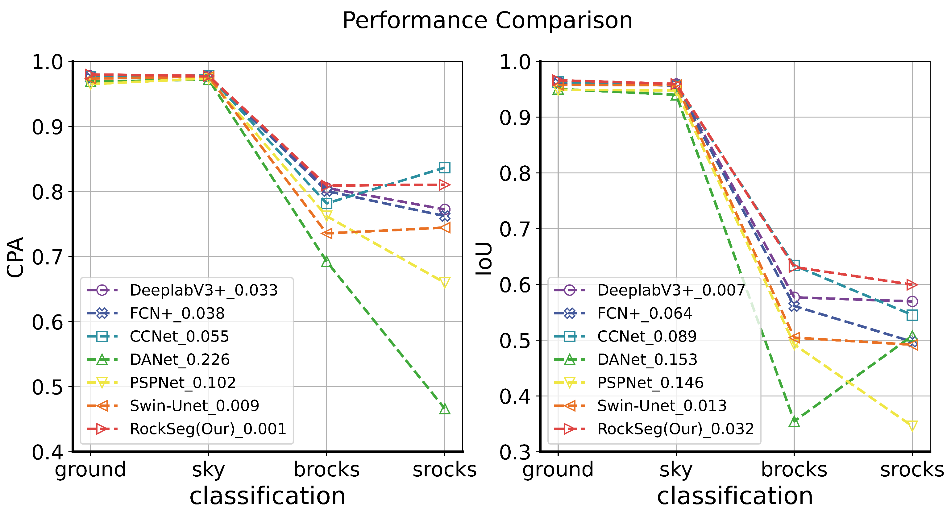
Furthermore, we used the CPA and IoU indicators to evaluate the different category detection results shown in Figure 4. The MoonData dataset has four categories including ground, sky, bigger rocks simplified “brocks”, and smaller rocks simplified “srocks”. In Figure 4, the horizontal axis represents four different categories and the vertical axis is the value of CPA and IoU, respectively. The legend represents different methods and ranges (R) in two categories of brocks and srocks; R is defined as

$$R=|R_{brocks}-R_{srocks}|$$

(11)

where $R_{brocks}$ and $R_{srocks}$ denote the accuracy score in brocks and srocks classes and R represents the difference between the two categories; the larger R, the more difficult it is to distinguish between the two categories; otherwise, the easier it is to distinguish between the two categories.

On the whole, we discovered that all compared methods could obtain better detection accuracy in the ground and sky categories, but the detection results of different models have a large gap in the brocks and srocks categories. For an input rock image of the Moon, the pixel ratio of the ground and sky is large, and the pixel ratio of the rocks is relatively small; there is an imbalance of categories in the MoonData data. In semantic segmentation, category objects with different pixel proportions in an image have different detection difficulties [55,56]. Category objects with small proportion pixels are difficult to distinguish, while category objects with multi-proportion pixels are relatively easy to distinguish [7]. So the ground and sky categories have a higher accuracy than the brocks and srocks categories in CPA and IoU evaluation.

From Figure 4, we can see that the DANet model had the worst classification results; the proposed model and the CCNet model had better detection accuracy than other methods. The DANet and PSPNet models obtained a large R between the brocks and srocks classifications; the accuracy range was 0.226 and 0.102 in CPA, and 0.153 and 0.146 in IoU, respectively. In the IoU evaluation, we found that RockSeg obtained the best scores in each classification; in particular, it achieved 63.11% and 59.94% IoU scores in brocks and srocks classifications, respectively. In the CPA evaluation, the RockSeg obtained high CPA values in ground, sky, and brocks classification, in which the brocks and srocks were 63.11% and 59.94%, respectively. The CCNet network also achieved the highest accuracy in the srocks class using the CPA evaluation, in which the brocks and srocks accuracy were 78.17% and 83.65%, respectively. However, RockSeg obtained a smaller R in CPA and IoU than the CCNet model. The accuracy range of RockSeg was only 0.001 compared to 0.055 for CCNet in the CPA evaluation and, in the IoU, the accuracy range of RockSeg was 0.032 and the R was lower than CCNet in the CPA and IoU evaluations. Thus, the proposed RockSeg is more robust than the CCNet model.

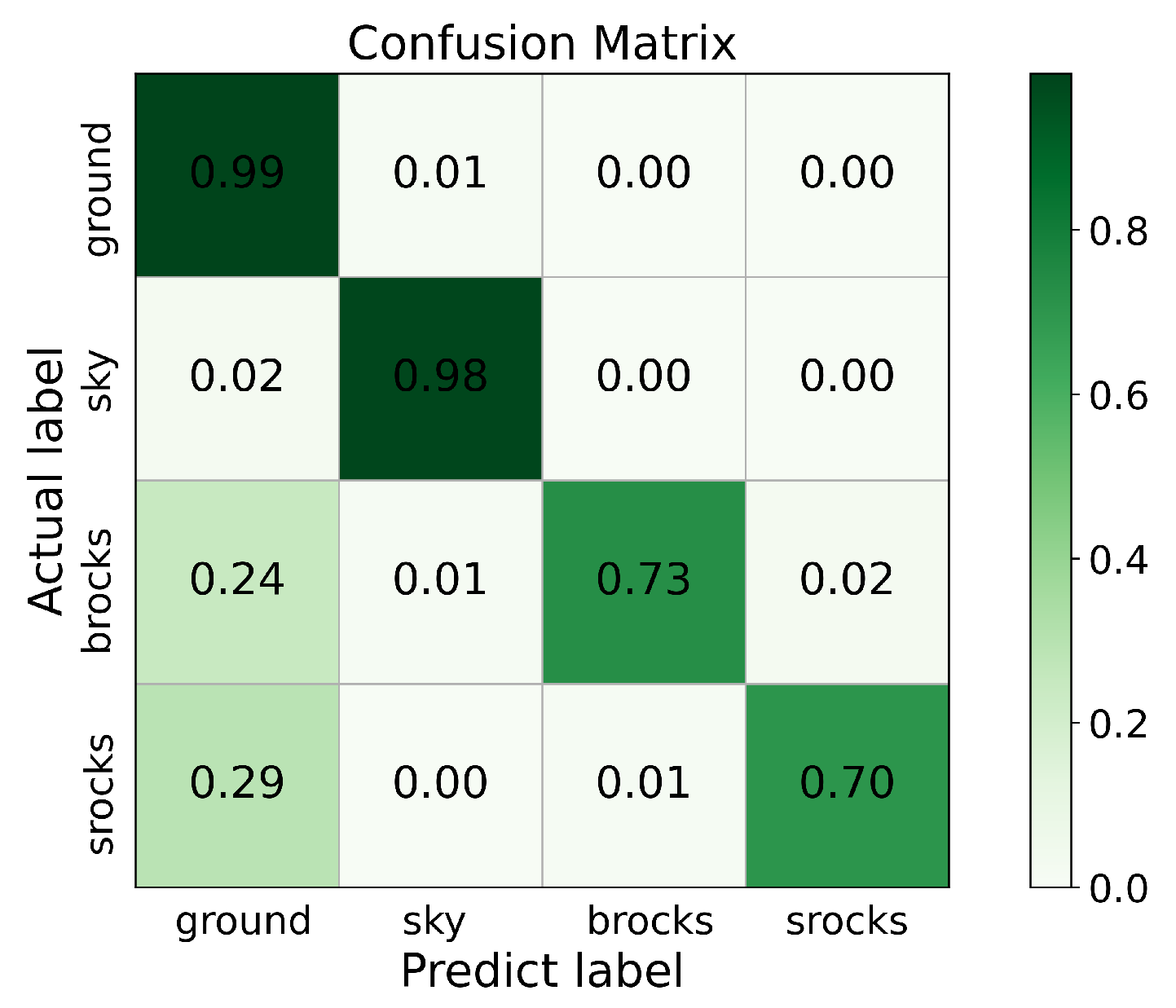
In addition, we show the confusion matrix of the probability of different categories being predicted in Figure 5. We can see that most pixels with ground and sky categories can be correctly classified; the probability of brocks being incorrectly classified as the ground category was 0.24 and the probability was only 0.02 of them being incorrectly classified as the srocks category. In the srocks category, there was only a probability of 0.29 and 0.01 of being incorrectly classified as the ground and brocks categories, respectively. Therefore, RockSeg has strong robustness for detecting deep space rocks; both large and small rocks can be detected correctly. Last, we show the visualization segmentation results of different methods on MarsData in Figure 6. There are five visualization segmentation results with different angles of sunlight and shadows in Figure 6. The yellow rectangle represents the contrast of the local details. Figure 6a,d,e denote the vision that follows the sunlight and Figure 6b,c are the visual angle against the sunlight on the surface of the Moon. When the sun’s rays shine perpendicular to the surface of the Moon, the rock shadows are small as shown in Figure 6d,e; otherwise, the rock shadows are big as shown in Figure 6a–c. We can see that the proposed RockSeg could accurately obtain segmentation results with different sunlight shadows and angles. Specifically, our model could clearly detect the boundary of the object compared to the other models and some small rock objects could also be accurately detected.

4.5.2. Results on MarsData

The comparison results with other methods on MarsData are shown in

Table 6. The comparison results with other methods on MarsData. The best result for each column is in bold.

Methods	PA (%)	MPA (%)	Recall (%)	MIoU (%)	FPS (HZ)
DeeplabV3+	98.72	97.12	98.51	97.12	54.13
FCN	98.52	98.29	98.29	98.29	55.83
CCNet	98.74	98.53	98.53	98.53	40.18
DANet	98.03	97.73	97.73	97.73	54.26
PSPNet	97.69	94.85	97.29	96.05	55.10
Swin-Unet	98.39	98.21	98.10	96.39	34.55
RockSeg (Ours)	98.91	98.78	98.73	97.54	55.18

; the bold denotes the best prediction accuracy. The MarsData has two categories, the background and rock objects. The pixel ratio of rocks and background is not much different, so it is relatively easy to segment them. We can see that the compared methods are all above 96% accuracy in the PA, Recall, and MIoU indicators. From Table 6, the FCN model obtained the best inference speed compared with other models and the precision of the PSPNet model was relatively low. Our proposed model obtained the best accuracy in each indicator compared to the other methods. Moreover, the proposed model achieved a high inference speed with low network parameters and computation complexity. Furthermore, we evaluated the CPA and IoU of different categories on MarsData; the results of different methods are shown in

Table 7. Comparisons of CPA and IoU for different methods on MarsData. The best result for each column is in bold.

Methods	CPA (%)		IoU (%)
	Ground	Rocks	Ground	Rocks
DeeplabV3+	99.01	98.12	98.14	96.10
FCN	98.88	97.76	97.84	95.50
CCnet	98.17	98.32	98.37	96.59
Danet	99.02	98.17	97.14	94.06
PSPNet	98.19	96.62	96.65	96.18
Swin-Unet	98.71	97.71	97.66	95.11
RockSeg (Ours)	99.16	98.23	98.41	96.68

. We found that R was small in the CPA and IoU evaluations for all compared models. Due to the classes being relatively balanced on MarsData data, they could be very well detected. We can see that the RockSeg model achieved the best score in the IoU evaluation and obtained the best PA value in ground classification compared to the other models. In deep space rock detection, our proposed model had excellent portability and robustness.

By comprehensive feature extraction and rich semantic feature fusion, the proposed model could realize high-precision detection. The proposed RockSeg network used combining the CNN and vision transformer to extract the rock features, in which the CNN network is advantageous in obtaining local multiscale context features and the vision transformer block is more suitable for capturing global features. The local and global rock features were fused to achieve a comprehensive feature extraction by the proposed hybrid network, which is beneficial for the detection of objects of different sizes. Moreover, the designed MSF module fused multiscale low-layer features to the output feature map which could improve the accuracy of the segmentation results. Furthermore, we eliminated the feature redundancy and overlap by manually adjusting the network parameters to achieve a lightweight network; see Section 4.6 for details of model parameters. Using the above policies, the proposed model could achieve high accuracy and inference speed under low computation complexity.

The visualization segmentation results of our model and the state-of-the-art methods on MarsData are shown in Figure 7. In the label image, we labeled the object rock as green and the other compared segment results as yellow for visual distinction. In the four image visualization segmentations, we discovered that all of the comparison models could accurately detect large rock objects. But, for some small gravel with burning in the soil and some dense rocks, it is relatively more difficult to distinguish and identify them than big rocks. In terms of accuracy and clarity of the border segmentation, the RockSeg results were finer and closer to the label image than the other model, and we used the red box in our model to show the finer boundary segmentation results. From the visualization segmentation results, we can see that the Swin-Unet, PSPNet, DANet, CCNet, and FCN models had poor detection results in small object detection; their segmentation results show that the target boundary was blurred and rough. In Figure 7b,d, we can see that the proposed model achieved accurate detection in big rocks, and also obtained accurate segmentation in some dense small rocks or small rocks buried in the soil.

4.5.3. Ablation Study

In this section, we ablated our network to validate the performance of the proposed model. The results of the ablation study are shown in

Table 8. The ablation results of our model on MoonData.

Model	MSF	T	PA (%)	MPA (%)	Recall (%)	MIoU (%)
RockSeg-no-MSF-T	–	–	97.12	88.70	84.39	77.93
RockSeg-T	–	✓	97.20	88.95	85.29	78.72
RockSeg-MSF	✓	–	97.18	88.89	85.10	78.56
RockSeg-MSF-T (Ours)	✓	✓	97.25	89.42	85.13	78.90

and the best value in each column is in bold. The MSF represents the multiscale low-level feature fusion module, the transformer block is simplified as T, the ✓ flag represents the module being used, and the – flag denotes the module not being used. In Table 8, we can see that our model obtained the best PA, MPA, and MioU compared to the other ablation models. The T module with a multi-headed attention mechanism could capture the global context information of the rock to improve the rock’s object detection accuracy. Thus, we discovered that RockSeg-T and the RockSeg-MSF-T achieved a higher accuracy in PA, MPA, Recall, and MIoU than RockSeg-no-MSF-T. Specifically, RockSeg-T obtained the best accuracy in Recall. The multiscale feature fusion module obtained the rich fusion feature maps $ms{f}_1$ and $ms{f}_2$; they were added to the output feature map using the upsampling process to accurately enhance the clarity of the semantic segmentation object boundary and improve the accuracy of segmentation. In Table 8, we found the RockSeg-MSF and RockSeg-MSF-T models also achieved an improvement over the RockSeg-no-MSF-T in the four evaluation indicators. On the whole, our model with T and MSF modules obtained the best performance in rock detection.

Furthermore, we show the visual ablation results of the MSF and T modules with the heatmap output shown in Figure 8. We compared the different channel activation statuses with the different models of RockSeg-no-MSF-T, RockSeg-T, RockSeg-MSF, and RockSeg-MSF-T. We used a blue–red color scheme to show the difference; the smaller the value, the closer it is to blue, the larger the value, the closer it is to red. In Figure 8, the top is the original rock image and label; Figure 8(1–6) show the two low-level feature maps $msf{}_1$ and $msf{}_2$, where Figure 8(1–3) denote the output results of $ms{f}_1$ and Figure 8(4–6) are the output results of $ms{f}_2$ with RockSeg-no-MSF-T, RockSeg-MSF, and RockSeg-MSF-T (our model). Figure 8a–c show the feature map output results of the transformer block using RockSeg-no-MSF-T, RockSeg-T, and RockSeg-MSF-T.

For the whole network structure, $msf{}_1$ is closer to the input network and $msf{}_2$ is relatively far from the network input. We can see that most information of the original image was retained in the activation output $msf{}_1$. From the activation output $msf{}_1$ and $msf{}_2$, we discovered that, as the number of layers increased, the activation output became more and more abstract. The density of activation decreased with the deepening of layers and the information about categories was increased. For example, the density of activation contrast, Figure 8(3) > Figure 8(6). In $msf{}_1$ and $msf{}_2$, we can see that RockSeg-MSF and RockSeg-MSF-T had more channel activation statuses than RockSeg-no-MSF-T; the proposed MSF module obtained more rich semantic information from the context. Due to the T module being far from the network input in the whole network structure, the activation output is very sparse and abstract as shown in Figure 8a–c. The RockSeg-T and RockSeg-MSF-T used multiple attention mechanisms to activate important information by setting different weights of attention. Thus, they had more red feature signatures than the RockSeg-no-MSF-T model in Figure 8. On the whole, from different output feature heatmaps, we found that the proposed semantic segmentation network based on a hybrid framework combining CNN and vision transformer, using an efficient feature extraction backbone and multiscale low-level feature fusion, had an excellent presentation of features to achieve good performance in rock detection.

4.6. Impact of Different Backbones and Parameters on Models

In this section, we discuss the parameter impact on our model and tune them with the MoonData data. The parameters contain the different backbone networks, the number of backbone layers, and the number of layers and heads of the T block. The tuning process is divided into three groups, denoted $gps$, $gps=\{gp1,gp2,gp3\}$. In the three groups, we kept the same decoder process, normalized the size of the feature map in downsampling to an input size of 1/16 times, and evaluated them by the indicators described in Section 4.3. The tuning results are shown in

Table 9. The impact of different backbones and parameters on models. The best result for each column in $gps$ is in bold.

gps	Backbone	nbs	MSF	T	PA (%)	MPA (%)	Recall (%)	MIoU (%)	FLOPs (M)	Params (G)	FPS (HZ)
gp1	Resnet-50	4	✓	✓	97.24	90.45	84.11	78.67	27.89	32.01	34.41
	Resnet-34	4	✓	✓	97.22	89.77	84.84	78.87	25.40	27.97	41.44
	Resnet-18	4	✓	✓	97.10	88.43	84.96	78.16	22.07	17.86	51.57
gp2	Resnet-34-4	4	✓	✓	97.22	89.77	84.84	78.87	25.40	27.97	41.44
	Resnet-34-3	3	✓	✓	97.24	88.8	85.96	79.12	22.00	14.72	43.57
	Resnet-34-2	2	✓	✓	97.25	89.42	85.13	78.90	20.29	7.94	52.90
gp3	Resnet-34-2-88	2	✓	–	97.17	88.98	85.29	78.73	21.10	11.09	52.83
	Resnet-34-2-44	2	✓	–	97.25	89.42	85.13	78.90	20.29	7.94	52.90
	Resnet-34-2-14	2	✓	–	97.21	88.97	85.38	78.80	20.29	7.94	52.47

. In Table 9, $nbs$ is the number of Resnet blocks. The backbone represents the network encoder with different modules and parameters, where MSF and T denote the multiscale low-level feature fusion module and vision transformer in the backbone, respectively. The T module has two import parameters, the number of heads represented by h and the depth of the transformer layer denoted d. The – represents the process of adjusting their parameters and the ✓ denotes using this module.

In $gp1$, we compared the impact of different Resnet backbones with four Resnet blocks on deep space rock detection. We combined Resnet-50, Resnet-34, and Resnet-18 with the T module as the backbone network separately, and used the same MSF module to decode the network. In $gp1$, we found Resnet-50 obtained the best PA and MPA with maximum parameters and a large amount of computation; Resnet-18 had low parameters, small amounts of computation, and high FPS. Resnet-34 achieved the best MIoU compared to Resnet-50 and Resnet-18; the detection accuracy in PA and MPA indicators was close to Resnet-50, and the model parameters and computations were close to Resnet-18. In order to balance the calculation complexity and accuracy of the rock detection model in a deep space environment with limited resources, we chose Resnet-34 as the backbone for our model. Too many feature extraction layers may cause feature redundancy and overlap. To obtain an efficient and lightweight feature extraction backbone network, after obtaining the Resnet-34 backbone, we tuned the number of Resnet blocks in the backbone to optimize our model. In $gp2$, Resnet-34-n represents the backbone with different numbers of Resnet blocks n, where $n=\{2,3,4\}$. We discovered that Resnet-34-2 with two Resnet blocks achieved better performance than the Resnet-34-4 and Resnet-34-3 models. In $gp2$, the Resnet-34-4 backbone network may have over-representation; the Resnet-34-2 backbone network achieved the appropriate representation for rock feature extraction. The Resnet-34-2 backbone could obtain the best PA, MPA, Recall, and MIoU score under low computation and parameters, and fast inference speed.

Last, in $gp3$, we test the impact on the proposed model by tuning the parameters of h and d in the T block. Resnet-34-2-$hd$ is composed of the Resnet-34-2 backbone network and the T module with h heads and d layers, where h is the number of heads, h = $\{1,4,8\}$; corresponding to the number of transformer layer d denotes d = $\{4,4,8\}$. In $gp3$, we found the parameter of h and d had little effect on the precision of the model, but the complexity of different parameters was different. In deep space, the probe carries limited resources, and onboard computation needs to satisfy not only high precision requirements but also low complexity requirements. We can see that Resnet-34-2-44 achieved a higher PA, MPA, and MIoU than other models with a faster inference speed. Thus, in this paper, in order to create a high accuracy and low complexity rock detection model, we chose the final Resnet-34-244 as the hybrid framework combining CNN and transformer for deep space rock images, which is based on the Resnet-34-2 backbone and the T module containing four heads and transformer layers.

5. Conclusions

In this paper, we proposed an efficient deep space rock detection network, named RockSeg, which is a novel semantic segmentation network based on a hybrid framework combining CNN and vision transformer for deep space rock images. The novel model contains an efficient backbone feature extraction block and a multiscale low-level feature fusion module for deep space rock detection. Firstly, to enhance the feature extraction, we used part of the Resnet-34 backbone and combined it with the visual transformer block as a new backbone network Resnet-T to extract the global context information of the rock. In addition, we proposed a simple and efficient multiscale low-level feature fusion module to obtain more rich detailed feature information. These rich features were fused to the output feature map in the network decoder to obtain a more fine-grained output result and improve the clarity of the semantic segmentation object boundary. Furthermore, the proposed model was applied to two rock segmentation datasets (lunar and Martian rock data) compared with six state-of-the-art segmentation models for deep space rock detection. The results demonstrated that the RockSeg model outperforms the state-of-the-Art rock detection methods; our model achieved good performance in deep space rock detection. In particular, on MoonData data, our model achieved accuracy up to 97.25% in the PA and 78.97% in the MIoU indicators with low parameters, smaller amount of computation, and high inference speeds.

In tuning the network process, we found the deeper network may not be a good choice to achieve the best performance; too many deep network structures may be redundant for feature extraction. The proposed hybrid network combines CNN and transformer; they need to play to their strengths to complement and integrate local and global context information. To obtain the best appropriate network structure, we manually adjust the network backbone structure and optimize the parameter configuration with coarse-grained parameter tuning. We employed a conventional backbone to achieve network feature extraction and used evaluation measures and visual heatmaps simultaneously to decide whether the network feature extraction is insufficient or redundant. Then, the network structure was suitably decreased and increased based on the qualitative and quantitative assessment results to meet the specific detection task. In the future, we need to further study how to integrate CNN and transformer network structures adaptively to remove redundant features and enhance the ability to capture local and global context information. Moreover, we will transplant and expand our work to the detection of deep space multi-category terrain segmentation, further improving the availability of the model in deep space.

References

1. Kilic, C.; Martinez, B.; Tatsch, C.A.; Beard, J.; Strader, J.; Das, S.; Ross, D.; Gu, Y.; Pereira, G.A.; Gross, J.N. NASA Space Robotics Challenge 2 Qualification Round: An Approach to Autonomous Lunar Rover Operations. IEEE Aerosp. Electron. Syst. Mag. 2021, 36, 24–41. [Google Scholar] [CrossRef]
2. Kuang, B.; Wisniewski, M.; Rana, Z.A.; Zhao, Y. Rock Segmentation in the Navigation Vision of the Planetary Rovers. Mathematics 2021, 9, 3048. [Google Scholar] [CrossRef]
3. Turan, E.; Speretta, S.; Gill, E. Autonomous navigation for deep space small satellites: Scientific and technological advances. Acta Astronaut. 2022, 193, 56–74. [Google Scholar] [CrossRef]
4. Furlán, F.; Rubio, E.; Sossa, H.; Ponce, V. Rock detection in a Mars-like environment using a CNN. In Proceedings of the Mexican Conference on Pattern Recognition; Springer: Queretaro, Mexico, 2019; pp. 149–158. [Google Scholar]
5. Liu, H.; Yao, M.; Xiao, X.; Xiong, Y. RockFormer: A U-shaped Transformer Network for Martian Rock Segmentation. IEEE Trans. Geosci. Remote Sens. 2023, 61, 1–16. [Google Scholar] [CrossRef]
6. Brockers, R.; Delaune, J.; Proença, P.; Schoppmann, P.; Domnik, M.; Kubiak, G.; Tzanetos, T. Autonomous safe landing site detection for a future mars science helicopter. In Proceedings of the 2021 IEEE Aerospace Conference (50100), Big Sky, MT, USA, 6–13 March 2021; pp. 1–8. [Google Scholar]
7. Fan, L.; Yuan, J.; Zha, K.; Wang, X. ELCD: Efficient Lunar Crater Detection Based on Attention Mechanisms and Multiscale Feature Fusion Networks from Digital Elevation Models. Remote Sens. 2022, 14, 5225. [Google Scholar] [CrossRef]
8. Ebadi, K.; Coble, K.; Kogan, D.; Atha, D.; Schwartz, R.; Padgett, C.; Vander Hook, J. Semantic mapping in unstructured environments: Toward autonomous localization of planetary robotic explorers. In Proceedings of the 2022 IEEE Aerospace Conference, Big Sky, MT, USA, 5–12 March 2022. [Google Scholar]
9. Ugenti, A.; Vulpi, F.; Domínguez, R.; Cordes, F.; Milella, A.; Reina, G. On the role of feature and signal selection for terrain learning in planetary exploration robots. J. Field Robot. 2022, 39, 355–370. [Google Scholar] [CrossRef]
10. Jiang, J.; Zeng, X.; Guzzetti, D.; You, Y. Path planning for asteroid hopping rovers with pre-trained deep reinforcement learning architectures. Acta Astronaut. 2020, 171, 265–279. [Google Scholar] [CrossRef]
11. Wang, W.; Lin, L.; Fan, Z.; Liu, J. Semi-Supervised Learning for Mars Imagery Classification and Segmentation. ACM Trans. Multimed. Comput. Commun. Appl. 2023, 19, 1–23. [Google Scholar] [CrossRef]
12. Gui, C.; Li, Z. An autonomous rock identification method for planetary exploration. In Emerging Technologies for Information Systems, Computing, and Management; Springer: Hangzhou, China, 2013; pp. 545–552. [Google Scholar]
13. Burl, M.C.; Thompson, D.R.; deGranville, C.; Bornstein, B.J. Rockster: Onboard rock segmentation through edge regrouping. J. Aerosp. Inf. Syst. 2016, 13, 329–342. [Google Scholar] [CrossRef]
14. Li, Y.; Wu, B. Analysis of rock abundance on lunar surface from orbital and descent images using automatic rock detection. J. Geophys. Res. Planets 2018, 123, 1061–1088. [Google Scholar] [CrossRef]
15. Xiao, X.; Cui, H.; Yao, M.; Tian, Y. Autonomous rock detection on mars through region contrast. Adv. Space Res. 2017, 60, 626–635. [Google Scholar] [CrossRef]
16. Xiao, X.; Cui, H.; Yao, M.; Fu, Y.; Qi, W. Auto rock detection via sparse-based background modeling for mars rover. In Proceedings of the 2018 IEEE Congress on Evolutionary Computation (CEC), Rio de Janeiro, Brazil, 8–13 July 2018; pp. 1–6. [Google Scholar]
17. Xiao, X.; Yao, M.; Liu, H.; Wang, J.; Zhang, L.; Fu, Y. A kernel-based multi-featured rock modeling and detection framework for a mars rover. IEEE Trans. Neural Netw. Learn. Syst. 2021, 34, 3335–3344. [Google Scholar] [CrossRef] [PubMed]
18. Goh, E.; Ward, I.R.; Vincent, G.; Pak, K.; Chen, J.; Wilson, B. Self-supervised Distillation for Computer Vision Onboard Planetary Robots. In Proceedings of the 2023 IEEE Aerospace Conference, Big Sky, MT, USA, 4–11 March 2023; pp. 1–11. [Google Scholar]
19. Huang, G.; Yang, L.; Cai, Y.; Zhang, D. Terrain classification-based rover traverse planner with kinematic constraints for Mars exploration. Planet. Space Sci. 2021, 209, 105371. [Google Scholar] [CrossRef]
20. Lateef, F.; Ruichek, Y. Survey on semantic segmentation using deep learning techniques. Neurocomputing 2019, 338, 321–348. [Google Scholar] [CrossRef]
21. Li, J.; Zi, S.; Song, R.; Li, Y.; Hu, Y.; Du, Q. A stepwise domain adaptive segmentation network with covariate shift alleviation for remote sensing imagery. IEEE Trans. Geosci. Remote Sens. 2022, 60, 1–15. [Google Scholar] [CrossRef]
22. Yu, F.; Koltun, V. Multi-scale context aggregation by dilated convolutions. arXiv 2015, arXiv:1511.07122. [Google Scholar]
23. He, K.; Zhang, X.; Ren, S.; Sun, J. Spatial pyramid pooling in deep convolutional networks for visual recognition. IEEE Trans. Pattern Anal. Mach. Intell. 2015, 37, 1904–1916. [Google Scholar] [CrossRef] [Green Version]
24. Zhao, H.; Shi, J.; Qi, X.; Wang, X.; Jia, J. Pyramid scene parsing network. In Proceedings of the IEEE Conference on Computer Vision and Pattern Recognition, Honolulu, HI, USA, 21–26 July 2017; pp. 2881–2890. [Google Scholar]
25. Chen, L.C.; Zhu, Y.; Papandreou, G.; Schroff, F.; Adam, H. Encoder-decoder with atrous separable convolution for semantic image segmentation. In Proceedings of the European Conference on Computer Vision (ECCV), Munich, Germany, 8–14 September 2018; pp. 833–851. [Google Scholar]
26. Yuan, Y.; Chen, X.; Wang, J. Object-contextual representations for semantic segmentation. In Proceedings of the Computer Vision—ECCV 2020: 16th European Conference, Glasgow, UK, 23–28 August 2020; Proceedings, Part VI 16. Springer: Glasgow, UK, 2020; pp. 173–190. [Google Scholar]
27. Liu, L.; Cheng, J.; Quan, Q.; Wu, F.X.; Wang, Y.P.; Wang, J. A survey on U-shaped networks in medical image segmentations. Neurocomputing 2020, 409, 244–258. [Google Scholar] [CrossRef]
28. Long, J.; Shelhamer, E.; Darrell, T. Fully convolutional networks for semantic segmentation. In Proceedings of the IEEE Conference on Computer Vision and Pattern Recognition, Boston, MA, USA, 7–12 June 2015; pp. 3431–3440. [Google Scholar]
29. Cao, H.; Wang, Y.; Chen, J.; Jiang, D.; Zhang, X.; Tian, Q.; Wang, M. Swin-unet: Unet-like pure transformer for medical image segmentation. In Proceedings of the European Conference on Computer Vision; Springer: Tel Aviv, Israel, 2022; pp. 205–218. [Google Scholar]
30. Li, H.; Qiu, L.; Li, Z.; Meng, B.; Huang, J.; Zhang, Z. Automatic Rocks Segmentation Based on Deep Learning for Planetary Rover Images. J. Aerosp. Inf. Syst. 2021, 18, 755–761. [Google Scholar] [CrossRef]
31. Ma, W.; Jiabin, Y.; Zha, k.; Fan, L. Onboard rock detection algorithm based on spiking neurnal network. In Computer Science; China Academic Journal Electronic Publish House: Beijing, China, 2023; pp. 98–104. [Google Scholar]
32. Sun, K.; Xiao, B.; Liu, D.; Wang, J. Deep high-resolution representation learning for human pose estimation. In Proceedings of the IEEE/CVF Conference on Computer Vision and Pattern Recognition, Long Beach, CA, USA, 15–20 June 2019; pp. 5693–5703. [Google Scholar]
33. Dai, Y.; Zheng, T.; Xue, C.; Zhou, L. SegMarsViT: Lightweight Mars Terrain Segmentation Network for Autonomous Driving in Planetary Exploration. Remote Sens. 2022, 14, 6297. [Google Scholar] [CrossRef]
34. Azkarate, M.; Gerdes, L.; Wiese, T.; Zwick, M.; Pagnamenta, M.; Hidalgo-Carrió, J.; Poulakis, P.; Pérez-del Pulgar, C.J. Design, testing, and evolution of mars rover testbeds: European space agency planetary exploration. IEEE Robot. Autom. Mag. 2022, 29, 10–23. [Google Scholar] [CrossRef]
35. Xiao, Z.; Su, Y.; Deng, Z.; Zhang, W. Efficient combination of CNN and transformer for dual-teacher uncertainty-guided semi-supervised medical image segmentation. Comput. Methods Programs Biomed. 2022, 226, 107099. [Google Scholar] [CrossRef]
36. Yang, H.; Yang, D. CSwin-PNet: A CNN-Swin Transformer combined pyramid network for breast lesion segmentation in ultrasound images. Expert Syst. Appl. 2023, 213, 119024. [Google Scholar] [CrossRef]
37. Dosovitskiy, A.; Beyer, L.; Kolesnikov, A.; Weissenborn, D.; Zhai, X.; Unterthiner, T.; Dehghani, M.; Minderer, M.; Heigold, G.; Gelly, S.; et al. An image is worth 16x16 words: Transformers for image recognition at scale. arXiv 2020, arXiv:2010.11929. [Google Scholar]
38. Zhang, Y.; Zhao, Y.; Dong, Y.; Du, B. Self-supervised Pre-training via Multi-modality Images with Transformer for Change Detection. IEEE Trans. Geosci. Remote Sens. 2023, 61, 1–11. [Google Scholar]
39. Zhang, X.; Cheng, S.; Wang, L.; Li, H. Asymmetric cross-attention hierarchical network based on CNN and transformer for bitemporal remote sensing images change detection. IEEE Trans. Geosci. Remote Sens. 2023, 61, 1–15. [Google Scholar] [CrossRef]
40. Luo, H.; Wang, P.; Xu, Y.; Ding, F.; Zhou, Y.; Wang, F.; Li, H.; Jin, R. Self-supervised pre-training for transformer-based person re-identification. arXiv 2021, arXiv:2111.12084. [Google Scholar]
41. Fang, J.; Lin, H.; Chen, X.; Zeng, K. A hybrid network of cnn and transformer for lightweight image super-resolution. In Proceedings of the IEEE/CVF Conference on Computer Vision and Pattern Recognition, New Orleans, LA, USA, 19–20 June 2022; pp. 1103–1112. [Google Scholar]
42. Wagstaff, K.; Lu, Y.; Stanboli, A.; Grimes, K.; Gowda, T.; Padams, J. Deep mars: Cnn classification of mars imagery for the pds imaging atlas. In Proceedings of the AAAI Conference on Artificial Intelligence, New Orleans, LA, USA, 2–7 February 2018; Volume 32. [Google Scholar]
43. Li, J.; Zhang, L.; Wu, Z.; Ling, Z.; Cao, X.; Guo, K.; Yan, F. Autonomous Martian rock image classification based on transfer deep learning methods. Earth Sci. Inform. 2020, 13, 951–963. [Google Scholar] [CrossRef]
44. Liu, H.; Yao, M.; Xiao, X.; Cui, H. A hybrid attention semantic segmentation network for unstructured terrain on Mars. Acta Astronaut. 2023, 204, 492–499. [Google Scholar] [CrossRef]
45. Liu, M.; Liu, J.; Ma, X. MRISNet: Deep-learning-based Martian instance segmentation against blur. Earth Sci. Inform. 2023, 16, 965–981. [Google Scholar] [CrossRef]
46. Panambur, T.; Chakraborty, D.; Meyer, M.; Milliken, R.; Learned-Miller, E.; Parente, M. Self-supervised learning to guide scientifically relevant categorization of martian terrain images. In Proceedings of the IEEE/CVF Conference on Computer Vision and Pattern Recognition, New Orleans, LA, USA, 19–20 June 2022; pp. 1322–1332. [Google Scholar]
47. Goh, E.; Chen, J.; Wilson, B. Mars terrain segmentation with less labels. In Proceedings of the 2022 IEEE Aerospace Conference (AERO), Big Sky, MT, USA, 5–12 March 2022; pp. 1–10. [Google Scholar]
48. He, K.; Zhang, X.; Ren, S.; Sun, J. Deep residual learning for image recognition. In Proceedings of the IEEE Conference on Computer Vision and Pattern Recognition, Las Vegas, NV, USA, 26 June–1 July 2016; pp. 770–778. [Google Scholar]
49. Xiong, R.; Yang, Y.; He, D.; Zheng, K.; Zheng, S.; Xing, C.; Zhang, H.; Lan, Y.; Wang, L.; Liu, T. On layer normalization in the transformer architecture. In Proceedings of the International Conference on Machine Learning, Virtual, 13–18 July 2020; pp. 10524–10533. [Google Scholar]
50. Zhu, Q.; Liao, C.; Hu, H.; Mei, X.; Li, H. MAP-Net: Multiple attending path neural network for building footprint extraction from remote sensed imagery. IEEE Trans. Geosci. Remote Sens. 2020, 59, 6169–6181. [Google Scholar] [CrossRef]
51. Hou, S.; Xiao, S.; Dong, W.; Qu, J. Multi-level features fusion via cross-layer guided attention for hyperspectral pansharpening. Neurocomputing 2022, 506, 380–392. [Google Scholar] [CrossRef]
52. Bock, S.; Weiß, M. A proof of local convergence for the Adam optimizer. In Proceedings of the 2019 International Joint Conference on Neural Networks (IJCNN), Budapest, Hungary, 14–19 July 2019; pp. 1–8. [Google Scholar]
53. Huang, Z.; Wang, X.; Huang, L.; Huang, C.; Wei, Y.; Liu, W. Ccnet: Criss-cross attention for semantic segmentation. In Proceedings of the IEEE/CVF International Conference on Computer Vision, Seoul, Republich of Korea, 27 October–2 November 2019; pp. 603–612. [Google Scholar]
54. Fu, J.; Liu, J.; Tian, H.; Li, Y.; Bao, Y.; Fang, Z.; Lu, H. Dual attention network for scene segmentation. In Proceedings of the IEEE/CVF Conference on Computer Vision and Pattern Recognition, Long Beach, CA, USA, 15–20 June 2019; pp. 3146–3154. [Google Scholar]
55. Hou, S.; Liu, Y.; Yang, Q. Real-time prediction of rock mass classification based on TBM operation big data and stacking technique of ensemble learning. J. Rock Mech. Geotech. Eng. 2022, 14, 123–143. [Google Scholar] [CrossRef]
56. Zhang, W.; Li, H.; Han, L.; Chen, L.; Wang, L. Slope stability prediction using ensemble learning techniques: A case study in Yunyang County, Chongqing, China. J. Rock Mech. Geotech. Eng. 2022, 14, 1089–1099. [Google Scholar] [CrossRef]
Figure 1. Framework overview of the proposed RockSeg.
Remotesensing 15 03935 g001
Figure 2. The backbone structure comparison of Resnet-34 and Resnet-T.
Remotesensing 15 03935 g002
Figure 3. Illustration of the multiscale low-level feature fusion.
Remotesensing 15 03935 g003
Figure 4. The comparison results of different network models with CPA and IoU on MoonData.
Remotesensing 15 03935 g004
Figure 5. The confusion matrix of the RockSeg model on MoonData.
Remotesensing 15 03935 g005
Figure 6. Comparison of the visualization segmentation results for different models on MoonData. (ae) show the different views of the rocks on the lunar surface from different Suns. (a,d,e) denote the vision that follows the sunlight, and (b,c) represent the visual angle against the sunlight.
Remotesensing 15 03935 g006
Figure 7. Comparison of the visualization segmentation results for different models on MarsData. (ad) show the different rocky features of the Martian surface. (a,b) represent the surface of Mars as composed of sparse mudstones and small boulders, and (c,d) denote dense large rocks and sandstone partially buried in the sand.
Remotesensing 15 03935 g007
Figure 8. Comparison of the visual results of the ablation study. (16) are the visual results of the MSF module with different models; (13) denote the output feature map of the m s f 1 module; (46) are the output feature map of the m s f 2 module. (ac) represent the output feature map of the T module with different models.
Remotesensing 15 03935 g008