
Synthetic Forest Stands and Point Clouds for Model Selection and Feature Space Comparison

 ,
,  , and
, and 
Abstract
:
1. Introduction
2. Background
3. Methods
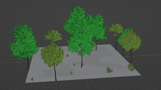
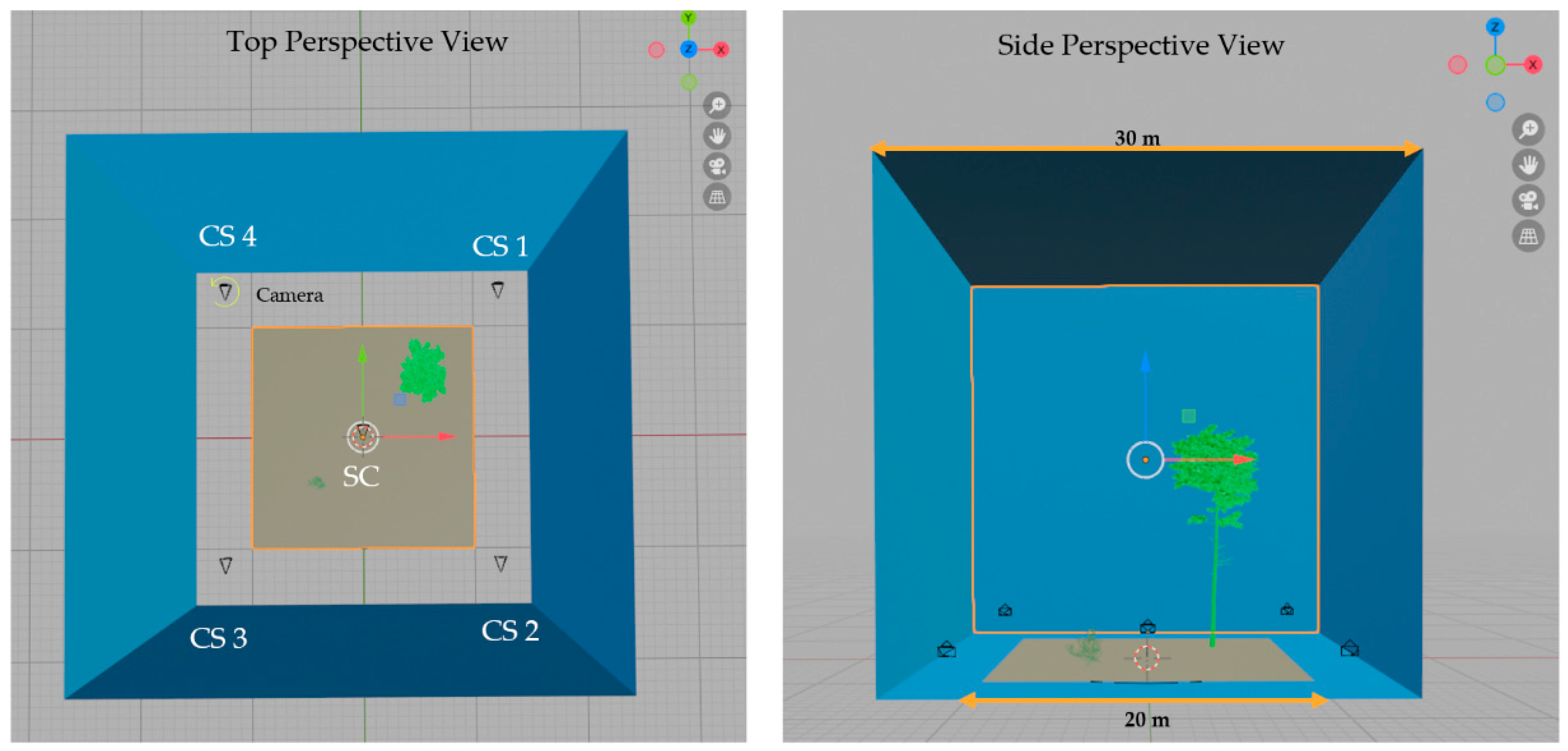
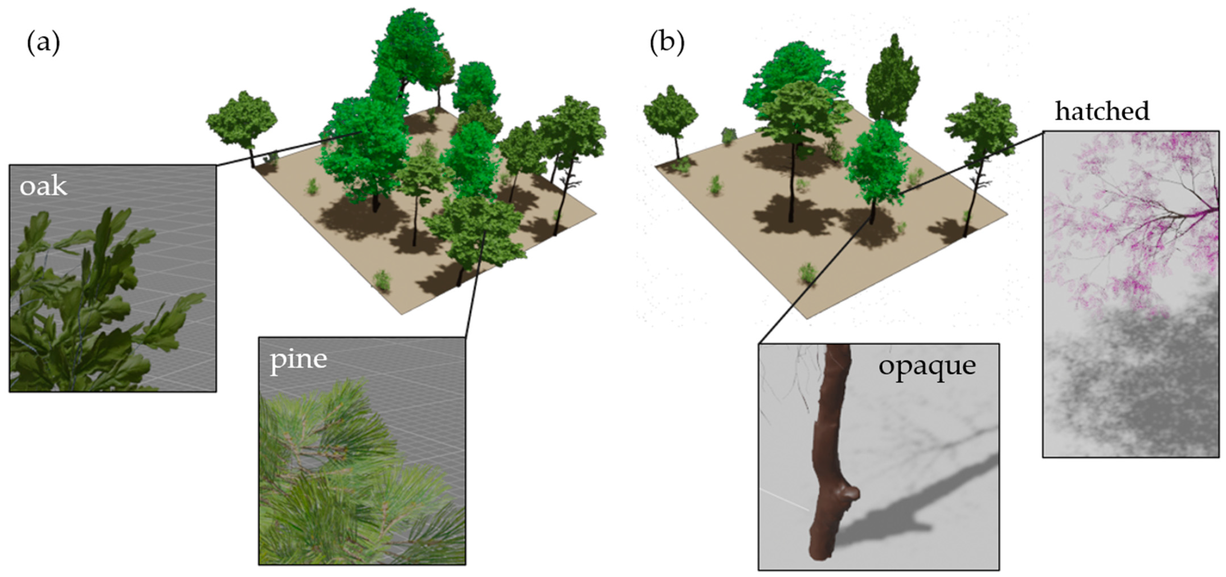
3.1. Synthetic Plot Generation
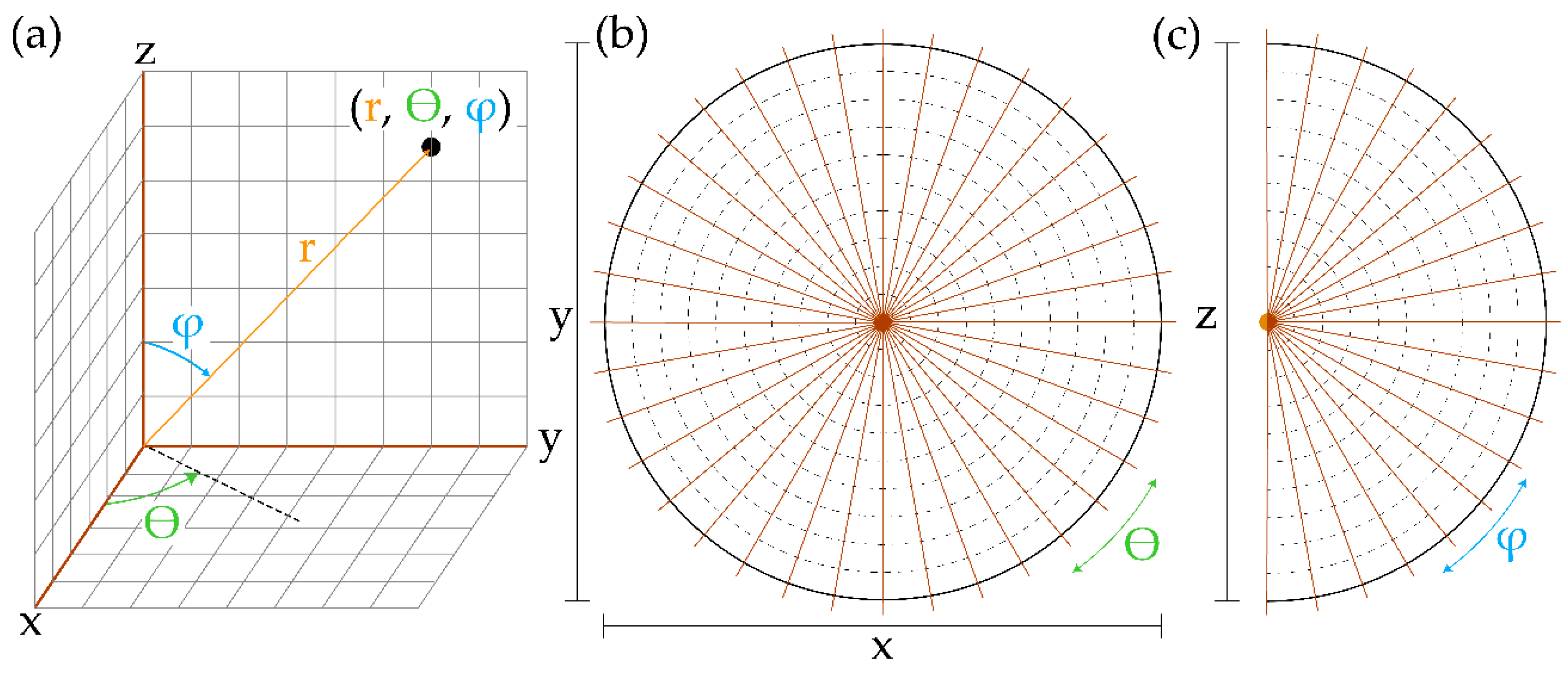
3.2. Simulated Lidar
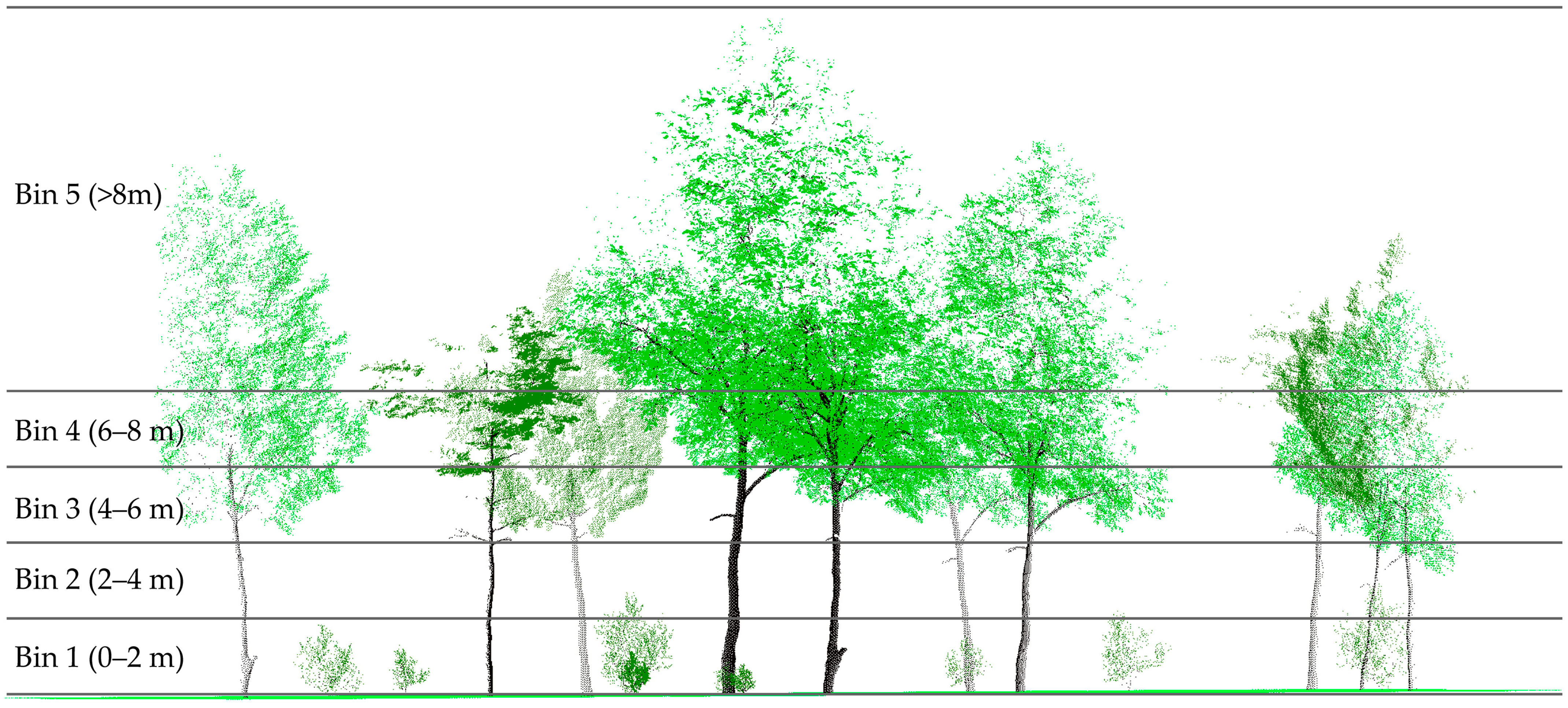
3.3. Measured Metrics
3.4. Modeling and Validation
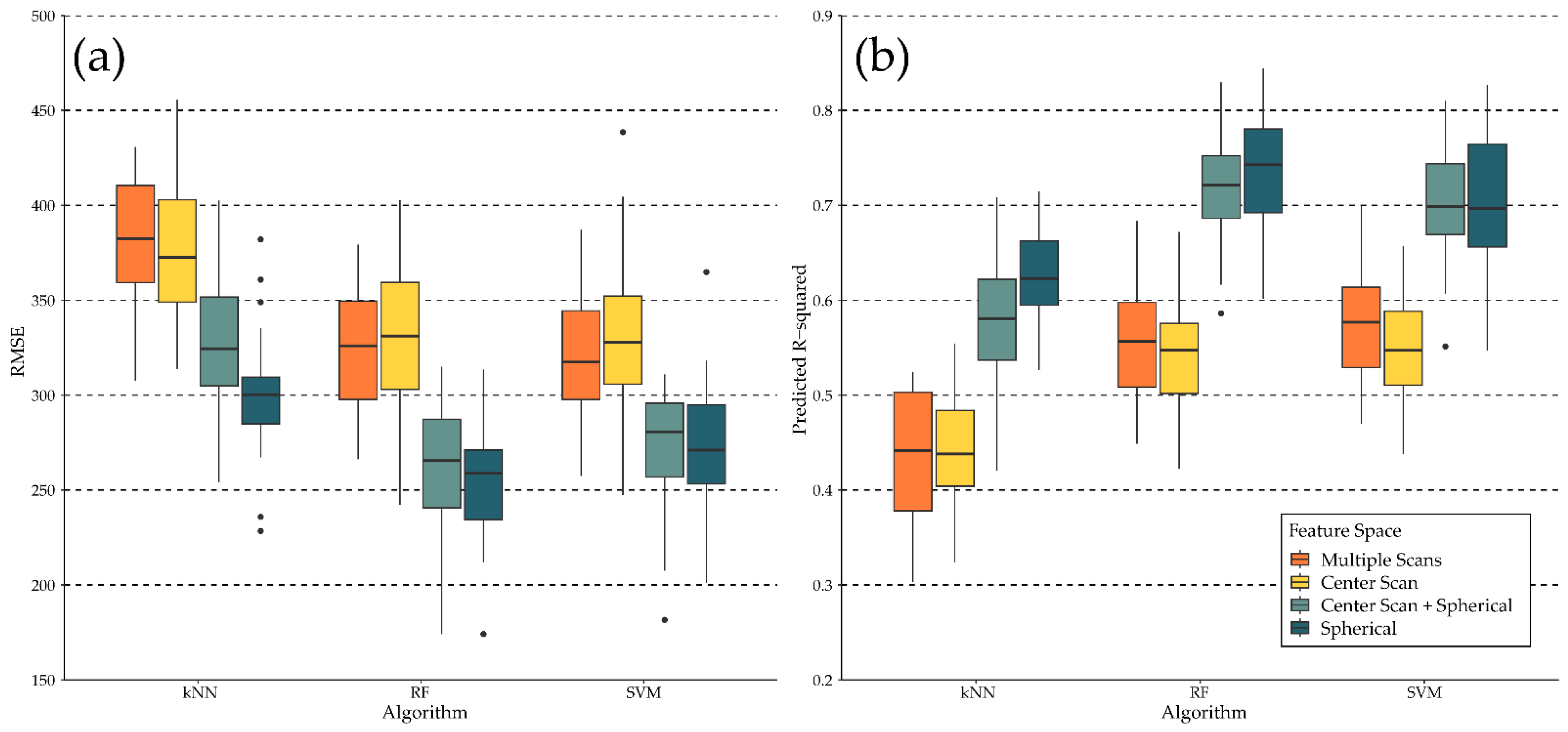
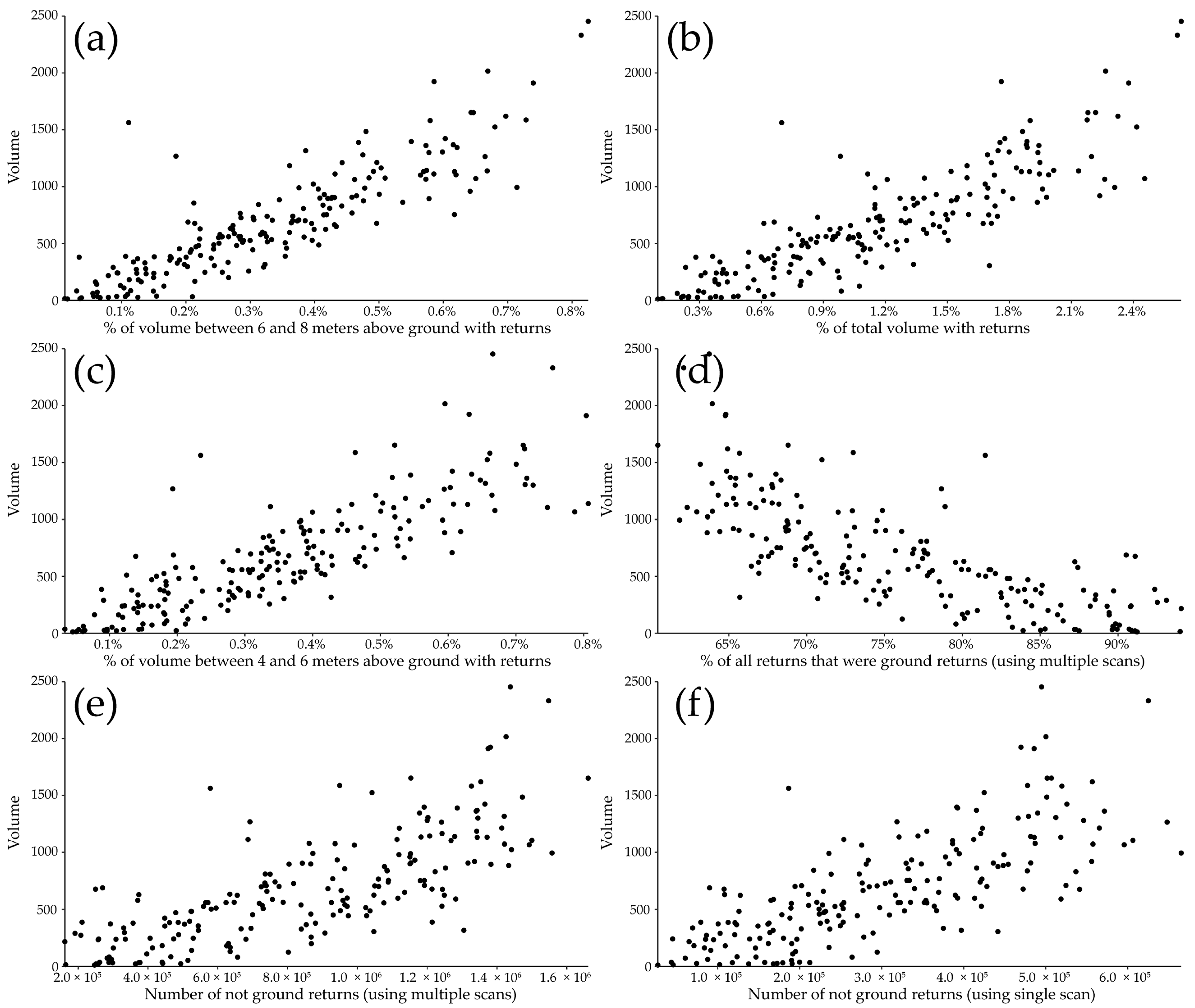
4. Results
5. Discussion and Future Work
6. Conclusions
Author Contributions
Funding
Data Availability Statement
Acknowledgments
Conflicts of Interest
References
- Aravanopoulos, F.A. Conservation and Monitoring of Tree Genetic Resources in Temperate Forests. Curr. For. Rep. 2016, 2, 119–129. [Google Scholar] [CrossRef]
- Hu, T.; Sun, Y.; Jia, W.; Li, D.; Zou, M.; Zhang, M. Study on the Estimation of Forest Volume Based on Multi-Source Data. Sensors 2021, 21, 7796. [Google Scholar] [CrossRef]
- Waser, L.T.; Fischer, C.; Wang, Z.; Ginzler, C. Wall-to-Wall Forest Mapping Based on Digital Surface Models from Image-Based Point Clouds and a NFI Forest Definition. Forests 2015, 6, 4510–4528. [Google Scholar] [CrossRef]
- Loudermilk, E.L.; O’Brien, J.J.; Mitchell, R.J.; Cropper, W.P.; Hiers, J.K.; Grunwald, S.; Grego, J.; Fernandez-Diaz, J.C.; Loudermilk, E.L.; O’Brien, J.J.; et al. Linking Complex Forest Fuel Structure and Fire Behaviour at Fine Scales. Int. J. Wildland Fire 2012, 21, 882–893. [Google Scholar] [CrossRef]
- Parker, G.G.; Harding, D.J.; Berger, M.L. A Portable LIDAR System for Rapid Determination of Forest Canopy Structure. J. Appl. Ecol. 2004, 41, 755–767. [Google Scholar] [CrossRef]
- Liao, K.; Li, Y.; Zou, B.; Li, D.; Lu, D. Examining the Role of UAV Lidar Data in Improving Tree Volume Calculation Accuracy. Remote Sens. 2022, 14, 4410. [Google Scholar] [CrossRef]
- Vagizov, M.; Istomin, E.; Miheev, V.; Potapov, A. Visual Digital Forest Model Based on a Remote Sensing Data and Forest Inventory Data. Remote Sens. 2021, 13, 4092. [Google Scholar]
- Andersen, H.-E.; McGaughey, R.J.; Reutebuch, S.E. Estimating Forest Canopy Fuel Parameters Using LIDAR Data. Remote Sens. Environ. 2005, 94, 441–449. [Google Scholar] [CrossRef]
- Skowronski, N.S.; Clark, K.L.; Duveneck, M.; Hom, J. Three-Dimensional Canopy Fuel Loading Predicted Using Upward and Downward Sensing LiDAR Systems. Remote Sens. Environ. 2011, 115, 703–714. [Google Scholar] [CrossRef]
- James, G.; Witten, D.; Hastie, T.; Tibshirani, R. An Introduction to Statistical Learning; Springer: Berlin/Heidelberg, Germany, 2013; Volume 112. [Google Scholar]
- Kuhn, M.; Johnson, K. Applied Predictive Modeling; Springer: New York, NY, USA, 2013; ISBN 978-1-4614-6848-6. [Google Scholar]
- Alkhatib, R.; Sahwan, W.; Alkhatieb, A.; Schütt, B. A Brief Review of Machine Learning Algorithms in Forest Fires Science. Appl. Sci. 2023, 13, 8275. [Google Scholar] [CrossRef]
- Maxwell, A.E.; Warner, T.A.; Fang, F. Implementation of Machine-Learning Classification in Remote Sensing: An Applied Review. Int. J. Remote Sens. 2018, 39, 2784–2817. [Google Scholar] [CrossRef]
- Celebi, M.E.; Aydin, K. Unsupervised Learning Algorithms; Springer: Berlin/Heidelberg, Germany, 2016; Volume 9. [Google Scholar]
- Hady, M.F.A.; Schwenker, F. Semi-Supervised Learning. Handb. Neural Inf. Process. 2013, 49, 215–239. [Google Scholar]
- Liu, W.; Liu, J.; Luo, B. Can Synthetic Data Improve Object Detection Results for Remote Sensing Images? arXiv 2020, arXiv:2006.05015. [Google Scholar]
- Fassnacht, F.E.; Latifi, H.; Hartig, F. Using Synthetic Data to Evaluate the Benefits of Large Field Plots for Forest Biomass Estimation with LiDAR. Remote Sens. Environ. 2018, 213, 115–128. [Google Scholar] [CrossRef]
- Coops, N.C.; Tompalski, P.; Goodbody, T.R.; Queinnec, M.; Luther, J.E.; Bolton, D.K.; White, J.C.; Wulder, M.A.; van Lier, O.R.; Hermosilla, T. Modelling Lidar-Derived Estimates of Forest Attributes over Space and Time: A Review of Approaches and Future Trends. Remote Sens. Environ. 2021, 260, 112477. [Google Scholar] [CrossRef]
- Sikkink, P.G.; Keane, R.E. A Comparison of Five Sampling Techniques to Estimate Surface Fuel Loading in Montane Forests. Int. J. Wildland Fire 2008, 17, 363–379. [Google Scholar] [CrossRef]
- Westfall, J.A.; Woodall, C.W. Measurement Repeatability of a Large-Scale Inventory of Forest Fuels. For. Ecol. Manag. 2007, 253, 171–176. [Google Scholar] [CrossRef]
- Xu, D.; Wang, H.; Xu, W.; Luan, Z.; Xu, X. LiDAR Applications to Estimate Forest Biomass at Individual Tree Scale: Opportunities, Challenges and Future Perspectives. Forests 2021, 12, 550. [Google Scholar] [CrossRef]
- Vandendaele, B.; Martin-Ducup, O.; Fournier, R.A.; Pelletier, G. Mobile and Terrestrial Laser Scanning for Tree Volume Estimation in Temperate Hardwood Forests. Available online: https://223.quebecconference.org/sites/223/files/documents/Extended_Abstract_Example_ICAG-CSRS_2022_Rev_02.pdf (accessed on 5 September 2023).
- Zhao, F.; Guo, Q.; Kelly, M. Allometric Equation Choice Impacts Lidar-Based Forest Biomass Estimates: A Case Study from the Sierra National Forest, CA. Agric. For. Meteorol. 2012, 165, 64–72. [Google Scholar] [CrossRef]
- Fehrmann, L.; Kleinn, C. General Considerations about the Use of Allometric Equations for Biomass Estimation on the Example of Norway Spruce in Central Europe. For. Ecol. Manag. 2006, 236, 412–421. [Google Scholar] [CrossRef]
- Basuki, T.; Van Laake, P.; Skidmore, A.; Hussin, Y. Allometric Equations for Estimating the above-Ground Biomass in Tropical Lowland Dipterocarp Forests. For. Ecol. Manag. 2009, 257, 1684–1694. [Google Scholar] [CrossRef]
- Henry, M.; Bombelli, A.; Trotta, C.; Alessandrini, A.; Birigazzi, L.; Sola, G.; Vieilledent, G.; Santenoise, P.; Longuetaud, F.; Valentini, R.; et al. GlobAllomeTree: International Platform for Tree Allometric Equations to Support Volume, Biomass and Carbon Assessment. Iforest-Biogeosci. For. 2013, 6, 326. [Google Scholar] [CrossRef]
- Gao, T.; Gao, Z.; Sun, B.; Qin, P.; Li, Y.; Yan, Z. An Integrated Method for Estimating Forest-Canopy Closure Based on UAV LiDAR Data. Remote Sens. 2022, 14, 4317. [Google Scholar] [CrossRef]
- Silva, A.G.P.; Görgens, E.B.; Campoe, O.C.; Alvares, C.A.; Stape, J.L.; Rodriguez, L.C.E. Assessing Biomass Based on Canopy Height Profiles Using Airborne Laser Scanning Data in Eucalypt Plantations. Sci. Agric. 2015, 72, 504–512. [Google Scholar] [CrossRef]
- Mayamanikandan, T.; Reddy, R.S.; Jha, C. Non-Destructive Tree Volume Estimation Using Terrestrial Lidar Data in Teak Dominated Central Indian Forests. In Proceedings of the 2019 IEEE Recent Advances in Geoscience and Remote Sensing: Technologies, Standards and Applications (TENGARSS), Kochi, India, 17–20 October 2019; pp. 100–103. [Google Scholar]
- Saarinen, N.; Kankare, V.; Vastaranta, M.; Luoma, V.; Pyörälä, J.; Tanhuanpää, T.; Liang, X.; Kaartinen, H.; Kukko, A.; Jaakkola, A.; et al. Feasibility of Terrestrial Laser Scanning for Collecting Stem Volume Information from Single Trees. ISPRS J. Photogramm. Remote Sens. 2017, 123, 140–158. [Google Scholar] [CrossRef]
- Gonsalves, M.O. A Comprehensive Uncertainty Analysis and Method of Geometric Calibration for a Circular Scanning Airborne Lidar; The University of Southern Mississippi: Hattiesburg, MS, USA, 2010; ISBN 1-124-40472-4. [Google Scholar]
- Gonzalez, P.; Asner, G.P.; Battles, J.J.; Lefsky, M.A.; Waring, K.M.; Palace, M. Forest Carbon Densities and Uncertainties from Lidar, QuickBird, and Field Measurements in California. Remote Sens. Environ. 2010, 114, 1561–1575. [Google Scholar] [CrossRef]
- Vicari, M.B.; Disney, M.; Wilkes, P.; Burt, A.; Calders, K.; Woodgate, W. Leaf and Wood Classification Framework for Terrestrial LiDAR Point Clouds. Methods Ecol. Evol. 2019, 10, 680–694. [Google Scholar] [CrossRef]
- Moorthy, I.; Miller, J.R.; Berni, J.A.J.; Zarco-Tejada, P.; Hu, B.; Chen, J. Field Characterization of Olive (Olea europaea L.) Tree Crown Architecture Using Terrestrial Laser Scanning Data. Agric. For. Meteorol. 2011, 151, 204–214. [Google Scholar] [CrossRef]
- Clark, M.L.; Clark, D.B.; Roberts, D.A. Small-Footprint Lidar Estimation of Sub-Canopy Elevation and Tree Height in a Tropical Rain Forest Landscape. Remote Sens. Environ. 2004, 91, 68–89. [Google Scholar] [CrossRef]
- Disney, M. Terrestrial LiDAR: A Three-Dimensional Revolution in How We Look at Trees. New Phytol. 2019, 222, 1736–1741. [Google Scholar] [CrossRef]
- Malambo, L.; Popescu, S.C.; Horne, D.W.; Pugh, N.A.; Rooney, W.L. Automated Detection and Measurement of Individual Sorghum Panicles Using Density-Based Clustering of Terrestrial Lidar Data. ISPRS J. Photogramm. Remote Sens. 2019, 149, 1–13. [Google Scholar] [CrossRef]
- Abegg, M.; Boesch, R.; Schaepman, M.E.; Morsdorf, F. Impact of Beam Diameter and Scanning Approach on Point Cloud Quality of Terrestrial Laser Scanning in Forests. IEEE Trans. Geosci. Remote Sens. 2021, 59, 8153–8167. [Google Scholar] [CrossRef]
- Rowell, E.; Loudermilk, E.L.; Hawley, C.; Pokswinski, S.; Seielstad, C.; Queen, L.l.; O’Brien, J.J.; Hudak, A.T.; Goodrick, S.; Hiers, J.K. Coupling Terrestrial Laser Scanning with 3D Fuel Biomass Sampling for Advancing Wildland Fuels Characterization. For. Ecol. Manag. 2020, 462, 117945. [Google Scholar] [CrossRef]
- Rowell, E.; Loudermilk, E.L.; Seielstad, C.; O’Brien, J.J. Using Simulated 3D Surface Fuelbeds and Terrestrial Laser Scan Data to Develop Inputs to Fire Behavior Models. Can. J. Remote Sens. 2016, 42, 443–459. [Google Scholar] [CrossRef]
- Rowell, E.M.; Seielstad, C.A.; Ottmar, R.D.; Rowell, E.M.; Seielstad, C.A.; Ottmar, R.D. Development and Validation of Fuel Height Models for Terrestrial Lidar—RxCADRE 2012. Int. J. Wildland Fire 2015, 25, 38–47. [Google Scholar] [CrossRef]
- Alonso-Benito, A.; Arroyo, L.; Arbelo, M.; Hernández-Leal, P. Fusion of WorldView-2 and LiDAR Data to Map Fuel Types in the Canary Islands. Remote Sens. 2016, 8, 669. [Google Scholar] [CrossRef]
- Calders, K.; Adams, J.; Armston, J.; Bartholomeus, H.; Bauwens, S.; Bentley, L.P.; Chave, J.; Danson, F.M.; Demol, M.; Disney, M.; et al. Terrestrial Laser Scanning in Forest Ecology: Expanding the Horizon. Remote Sens. Environ. 2020, 251, 112102. [Google Scholar] [CrossRef]
- Tao, S.; Labrière, N.; Calders, K.; Fischer, F.J.; Rau, E.-P.; Plaisance, L.; Chave, J. Mapping Tropical Forest Trees across Large Areas with Lightweight Cost-Effective Terrestrial Laser Scanning. Ann. For. Sci. 2021, 78, 103. [Google Scholar] [CrossRef]
- Frazer, G.W.; Magnussen, S.; Wulder, M.A.; Niemann, K.O. Simulated Impact of Sample Plot Size and Co-Registration Error on the Accuracy and Uncertainty of LiDAR-Derived Estimates of Forest Stand Biomass. Remote Sens. Environ. 2011, 115, 636–649. [Google Scholar] [CrossRef]
- Wang, L.; Birt, A.G.; Lafon, C.W.; Cairns, D.M.; Coulson, R.N.; Tchakerian, M.D.; Xi, W.; Popescu, S.C.; Guldin, J.M. Computer-Based Synthetic Data to Assess the Tree Delineation Algorithm from Airborne LiDAR Survey. Geoinformatica 2013, 17, 35–61. [Google Scholar] [CrossRef]
- Jiang, K.; Chen, L.; Wang, X.; An, F.; Zhang, H.; Yun, T. Simulation on Different Patterns of Mobile Laser Scanning with Extended Application on Solar Beam Illumination for Forest Plot. Forests 2022, 13, 2139. [Google Scholar] [CrossRef]
- White, J.C.; Coops, N.C.; Wulder, M.A.; Vastaranta, M.; Hilker, T.; Tompalski, P. Remote Sensing Technologies for Enhancing Forest Inventories: A Review. Can. J. Remote Sens. 2016, 42, 619–641. [Google Scholar] [CrossRef]
- Yun, T.; Cao, L.; An, F.; Chen, B.; Xue, L.; Li, W.; Pincebourde, S.; Smith, M.J.; Eichhorn, M.P. Simulation of Multi-Platform LiDAR for Assessing Total Leaf Area in Tree Crowns. Agric. For. Meteorol. 2019, 276, 107610. [Google Scholar] [CrossRef]
- Goodwin, N.; Coops, N.; Culvenor, D. Development of a Simulation Model to Predict LiDAR Interception in Forested Environments. Remote Sens. Environ. 2007, 111, 481–492. [Google Scholar] [CrossRef]
- Sun, G.; Ranson, K.J. Modeling Lidar Returns from Forest Canopies. IEEE Trans. Geosci. Remote Sens. 2000, 38, 2617–2626. [Google Scholar] [CrossRef]
- Disney, M.I.; Kalogirou, V.; Lewis, P.; Prieto-Blanco, A.; Hancock, S.; Pfeifer, M. Simulating the Impact of Discrete-Return Lidar System and Survey Characteristics over Young Conifer and Broadleaf Forests. Remote Sens. Environ. 2010, 114, 1546–1560. [Google Scholar] [CrossRef]
- Loidi Arregui, J.J.; Marcenò, C. The Temperate Deciduous Forests of the Northern Hemisphere. A Review. Mediterr. Bot. 2022, 43, e75527. [Google Scholar] [CrossRef]
- Hartley, F.M.; Maxwell, A.E.; Landenberger, R.E.; Bortolot, Z.J. Forest Type Differentiation Using GLAD Phenology Metrics, Land Surface Parameters, and Machine Learning. Geographies 2022, 2, 491–515. [Google Scholar] [CrossRef]
- Zhang, Z.; Li, X.; Liu, H. Biophysical Feedback of Forest Canopy Height on Land Surface Temperature over Contiguous United States. Environ. Res. Lett. 2022, 17, 034002. [Google Scholar] [CrossRef]
- Fei, S.; Yang, P. Forest Composition Change in the Eastern United States. In Proceedings of the 17th Central Hardwood Forest Conference, Lexington, KY, USA, 5–7 April 2010. [Google Scholar]
- U.S. National Park Service Eastern Deciduous Forest. Available online: https://www.nps.gov/im/ncrn/eastern-deciduous-forest.htm (accessed on 29 October 2022).
- Olson, D.M.; Dinerstein, E. The Global 200: Priority Ecoregions for Global Conservation. Ann. Mo. Bot. Gard. 2002, 89, 199–224. [Google Scholar] [CrossRef]
- van der Walt, L. What Are Meshes in 3D Modeling? Available online: http://wedesignvirtual.com/what-are-meshes-in-3d-modeling/ (accessed on 30 October 2022).
- Estornell, J.; Ruiz, L.A.; Velázquez-Martí, B.; Hermosilla, T. Analysis of the Factors Affecting LiDAR DTM Accuracy in a Steep Shrub Area. Int. J. Digit. Earth 2011, 4, 521–538. [Google Scholar] [CrossRef]
- Campbell, M.J.; Dennison, P.E.; Hudak, A.T.; Parham, L.M.; Butler, B.W. Quantifying Understory Vegetation Density Using Small-Footprint Airborne Lidar. Remote Sens. Environ. 2018, 215, 330–342. [Google Scholar] [CrossRef]
- Contreras, M.A.; Staats, W.; Yiang, J.; Parrott, D. Quantifying the Accuracy of LiDAR-Derived DEM in Deciduous Eastern Forests of the Cumberland Plateau. J. Geogr. Inf. Syst. 2017, 9, 339–353. [Google Scholar] [CrossRef]
- Admin_Stanpro Reflection of Light: What Is Specular Reflection. Stanpro. 2018. Available online: https://www.standardpro.com/what-is-specular-reflection/ (accessed on 5 September 2023).
- Poirier-Quinot, D.; Noisternig, M.; Katz, B.F. EVERTims: Open Source Framework for Real-Time Auralization in VR. In Proceedings of the 12th International Audio Mostly Conference on Augmented and Participatory Sound and Music Experiences; 2017; pp. 1–5. Available online: https://dl.acm.org/doi/10.1145/3123514.3123559 (accessed on 5 September 2023).
- Reitmann, S.; Neumann, L.; Jung, B. BLAINDER—A Blender AI Add-on for Generation of Semantically Labeled Depth-Sensing Data. Sensors 2021, 21, 2144. [Google Scholar] [CrossRef] [PubMed]
- Gusmão, G.F.; Barbosa, C.R.H.; Raposo, A.B.; de Oliveira, R.C. A LiDAR System Simulator Using Parallel Raytracing and Validated by Comparison with a Real Sensor. J. Phys. Conf. Ser. 2021, 1826, 012002. [Google Scholar] [CrossRef]
- Scratchpixel An Overview of the Ray-Tracing Rendering Technique. Available online: https://www.scratchapixel.com/lessons/3d-basic-rendering/ray-tracing-overview/ray-tracing-rendering-technique-overview (accessed on 3 November 2022).
- Disney, M.; Lewis, P.; North, P. Monte Carlo Ray Tracing in Optical Canopy Reflectance Modelling. Remote Sens. Rev. 2000, 18, 163–196. [Google Scholar] [CrossRef]
- R Core Team. R: A Language and Environment for Statistical Computing; R Foundation for Statistical Computing: Vienna, Austria, 2020. [Google Scholar]
- Roussel, J.-R.; Auty, D. Airborne LiDAR Data Manipulation and Visualization for Forestry Applications; R Package Version 3.1. 2022. Available online: https://cran.r-project.org/package=lidR (accessed on 5 September 2023).
- Roussel, J.-R.; Auty, D.; Coops, N.C.; Tompalski, P.; Goodbody, T.R.; Meador, A.S.; Bourdon, J.-F.; De Boissieu, F.; Achim, A. LidR: An R Package for Analysis of Airborne Laser Scanning (ALS) Data. Remote Sens. Environ. 2020, 251, 112061. [Google Scholar] [CrossRef]
- Roussel, J.-R.; De Boissieu, F. rlas: Read and Write ‘las’ and ‘laz’ Binary File Formats Used for Remote Sensing Data; R package version 1.6.2. 2023. Available online: https://CRAN.R-project.org/package=rlas (accessed on 5 September 2023).
- Paula, C. Sanematsu Interactive 3D Visualization and Post-Processing Analysis of Vertex-Based Unstructured Polyhedral Meshes with ParaView. bioRxiv 2021. [Google Scholar] [CrossRef]
- Brownlee, C.; DeMarle, D. Fast Volumetric Gradient Shading Approximations for Scientific Ray Tracing. In Ray Tracing Gems II: Next Generation Real-Time Rendering with DXR, Vulkan, and OptiX; Marrs, A., Shirley, P., Wald, I., Eds.; Apress: Berkeley, CA, USA, 2021; pp. 725–733. ISBN 978-1-4842-7185-8. [Google Scholar]
- Lary, D.J.; Alavi, A.H.; Gandomi, A.H.; Walker, A.L. Machine Learning in Geosciences and Remote Sensing. Geosci. Front. 2016, 7, 3–10. [Google Scholar] [CrossRef]
- Yu, P. Research and Prediction of Ecological Footprint Using Machine Learning: A Case Study of China. In Proceedings of the 2022 International Conference on Big Data, Information and Computer Network (BDICN), Sanya, China, 20–22 January 2022; pp. 112–116. [Google Scholar]
- Hamilton, D.; Pacheco, R.; Myers, B.; Peltzer, B. KNN vs. SVM: A Comparison of Algorithms. In Proceedings of the Fire Continuum-Preparing for the Future of Wildland Fire, Missoula, MT, USA, 21–24 May 2018; Hood, S.M., Drury, S., Steelman, T., Steffens, R., Eds.; Proceedings RMRS-P-78. Department of Agriculture, Forest Service, Rocky Mountain Research Station: Fort Collins, CO, USA, 2020; Volume 78, pp. 95–109. [Google Scholar]
- Fletcher, T. Support Vector Machines Explained. Tutor. Pap. 2009, 1–19. [Google Scholar]
- Duda, R.O.; Hart, P.E. Pattern Classification; John Wiley & Sons: Hoboken, NJ, USA, 2006; ISBN 81-265-1116-8. [Google Scholar]
- Wright, M.N.; Ziegler, A. Ranger: A Fast Implementation of Random Forests for High Dimensional Data in C++ and R. J. Stat. Softw. 2017, 77, 1–17. [Google Scholar] [CrossRef]
- Kuhn, M. Caret: Classification and Regression Training; R Package Version 6.0-90. 2021. Available online: https://CRAN.R-project.org/package=caret (accessed on 5 September 2023).
- Karatzoglou, A.; Smola, A.; Hornik, K.; Karatzoglou, M.A.; SparseM, S.; Yes, L.; The Kernlab Package. Kernel-Based Machine Learning Lab. R Package Version 0.9.-22. 2017. Available online: https://cran.r-project.org/web/packages/kernlab (accessed on 4 November 2015).
- Belgiu, M.; Drăguţ, L. Random Forest in Remote Sensing: A Review of Applications and Future Directions. ISPRS J. Photogramm. Remote Sens. 2016, 114, 24–31. [Google Scholar] [CrossRef]
- Kuhn, M.; Vaughan, D. Yardstick: Tidy Characterizations of Model Performance. 2021. Available online: https://cran.r-project.org/web/packages/yardstick/index.html (accessed on 5 September 2023).
- Hudak, A.T.; Crookston, N.L.; Evans, J.S.; Hall, D.E.; Falkowski, M.J. Nearest Neighbor Imputation of Species-Level, Plot-Scale Forest Structure Attributes from LiDAR Data. Remote Sens. Environ. 2008, 112, 2232–2245. [Google Scholar] [CrossRef]
- Hernando, A.; Sobrini, I.; Velázquez, J.; García-Abril, A. The Importance of Protected Habitats and LiDAR Data Availability for Assessing Scenarios of Land Uses in Forest Areas. Land Use Policy 2022, 112, 105859. [Google Scholar] [CrossRef]
- Hyyppä, J.; Hyyppä, H.; Leckie, D.; Gougeon, F.; Yu, X.; Maltamo, M. Review of Methods of Small-footprint Airborne Laser Scanning for Extracting Forest Inventory Data in Boreal Forests. Int. J. Remote Sens. 2008, 29, 1339–1366. [Google Scholar] [CrossRef]
- Watt, P.J.; Donoghue, D.N.M. Measuring Forest Structure with Terrestrial Laser Scanning. Int. J. Remote Sens. 2005, 26, 1437–1446. [Google Scholar] [CrossRef]
- Wilkes, P.; Lau, A.; Disney, M.; Calders, K.; Burt, A.; Gonzalez de Tanago, J.; Bartholomeus, H.; Brede, B.; Herold, M. Data Acquisition Considerations for Terrestrial Laser Scanning of Forest Plots. Remote Sens. Environ. 2017, 196, 140–153. [Google Scholar] [CrossRef]
- Lovell, J.; Jupp, D.; Newnham, G.; Coops, N.; Culvenor, D. Simulation Study for Finding Optimal Lidar Acquisition Parameters for Forest Height Retrieval. For. Ecol. Manag. 2005, 214, 398–412. [Google Scholar] [CrossRef]


| Model | Mi * Height (Z) | Mi Crown Dimensions (X, Y) | Randomization Threshold (min, max) | Random Rotation (X, Y, Z) |
|---|---|---|---|---|
| Pine 1 | 15.0 m | 5.0 m, 6.0 m | 60%, 130% | (±4°, ±4°, 360°) |
| Pine 2 | 10.0 m | 4.0 m, 4.5 m | 60%, 130% | (±4°, ±4°, 360°) |
| Oak | 12.0 m | 5.0 m, 6.0 m | 60%, 130% | (±4°, ±4°, 360°) |
| Maple | 8.0 m | 3.8 m, 3.8 m | 50%, 150% | (±4°, ±4°, 360°) |
| Shrub | 1.5 m | 2.2 m, 1.8 m | 40%, 150% | (±4°, ±4°, 360°) |
| Metric Subset | Variable | Count of Variables |
|---|---|---|
| All returns | Ground return count | 2 |
| Not ground count | 2 | |
| Percent ground | 2 | |
| All non-ground returns | Mean Z | 2 |
| Median Z | 2 | |
| Standard deviation Z | 2 | |
| Skewness Z | 2 | |
| Kurtosis Z | 2 | |
| Percentiles (10% to 9% by 10%) | 18 | |
| Non-ground returns by height strata | Return count | 10 |
| Percent of all non-ground returns in strata | 10 | |
| Mean Z | 10 | |
| Median Z | 10 | |
| Standard Deviation Z | 10 | |
| Skewness Z | 10 | |
| Kurtosis Z | 10 | |
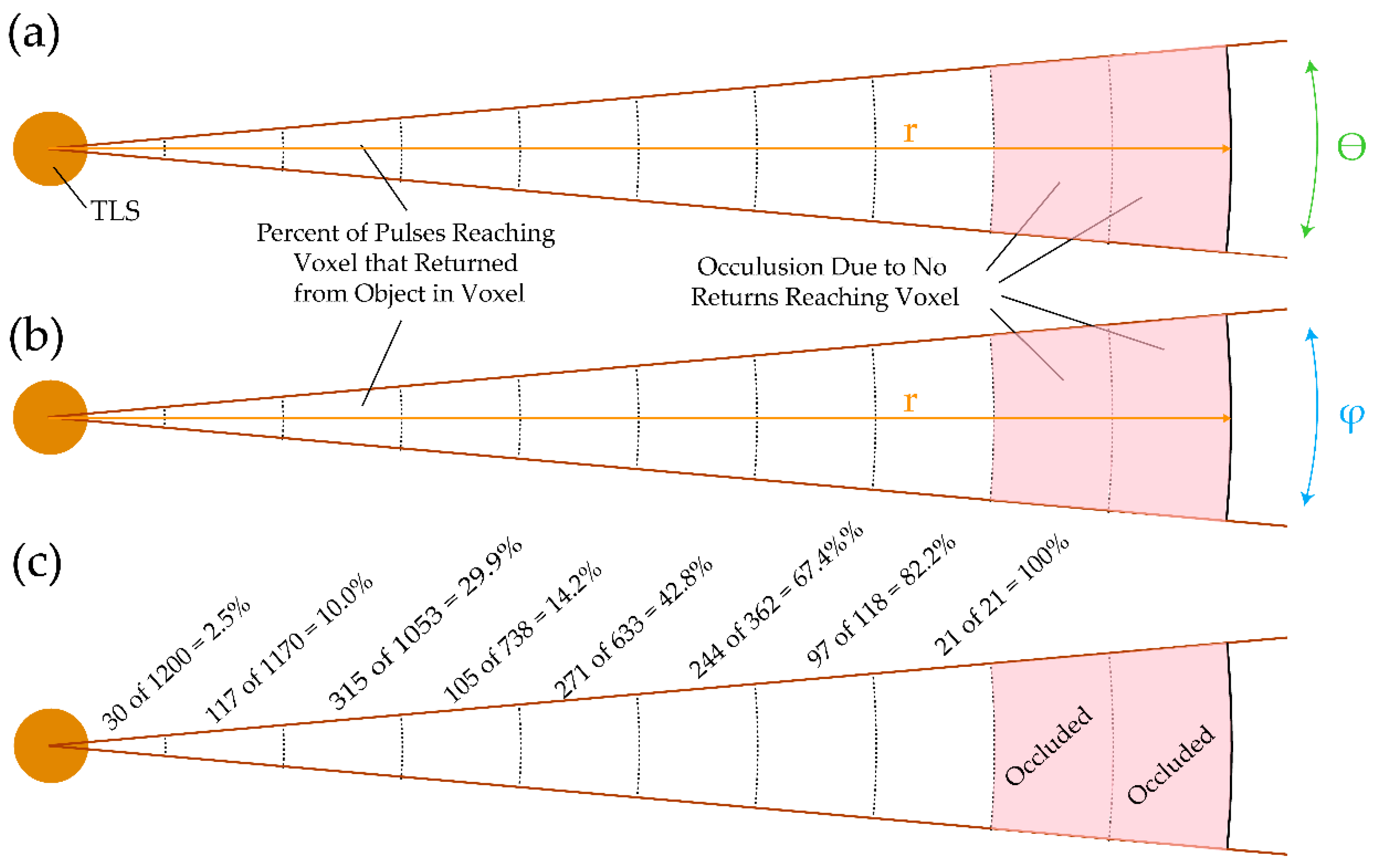
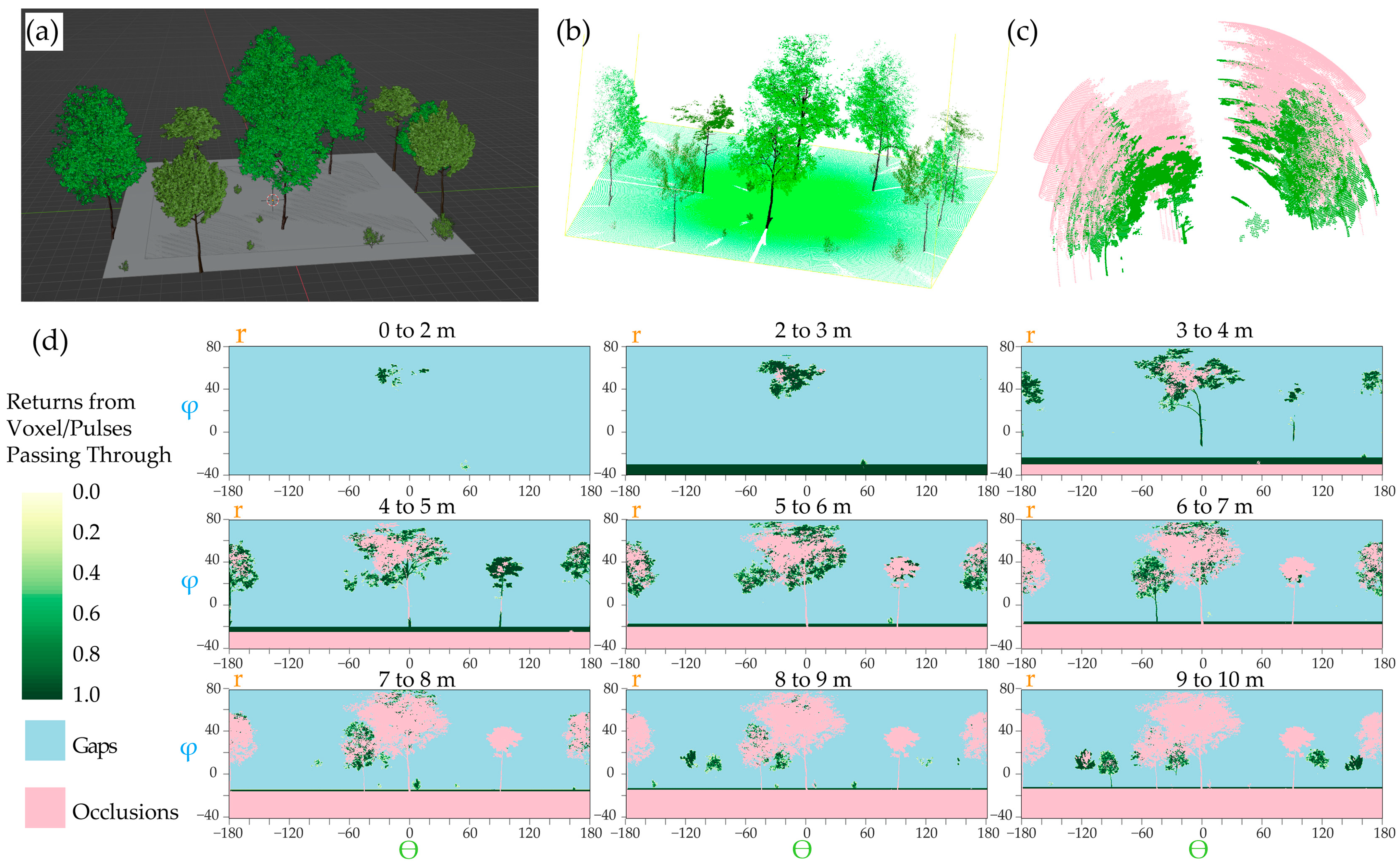
| Spherical-based (total and by height bin) | Percent of area occluded | 6 |
| Percent of area with returns | 6 | |
| Percent of area with gaps | 6 | |
| Spherical-based (by height bin) | Mean proportion of pulses returned | 5 |
| Total | 127 |
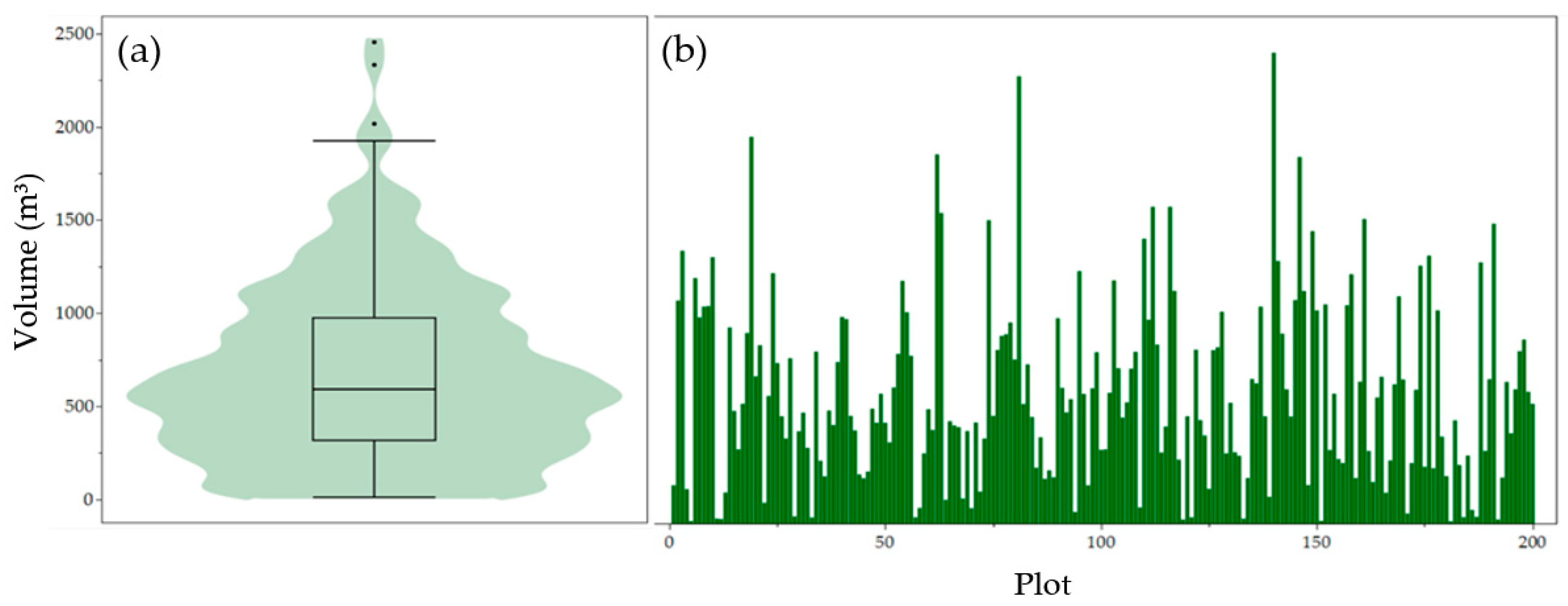
| Descriptive Statistic | Volume (m3) |
|---|---|
| Minimum | 11.72 |
| Maximum | 2453.66 |
| 1st Quartile | 324.56 |
| Median | 593.56 |
| 3rd Quartile | 964.19 |
| Mean | 679.22 |
| Standard deviation | 475.44 |
| Interquartile range (IQR) | 639.63 |
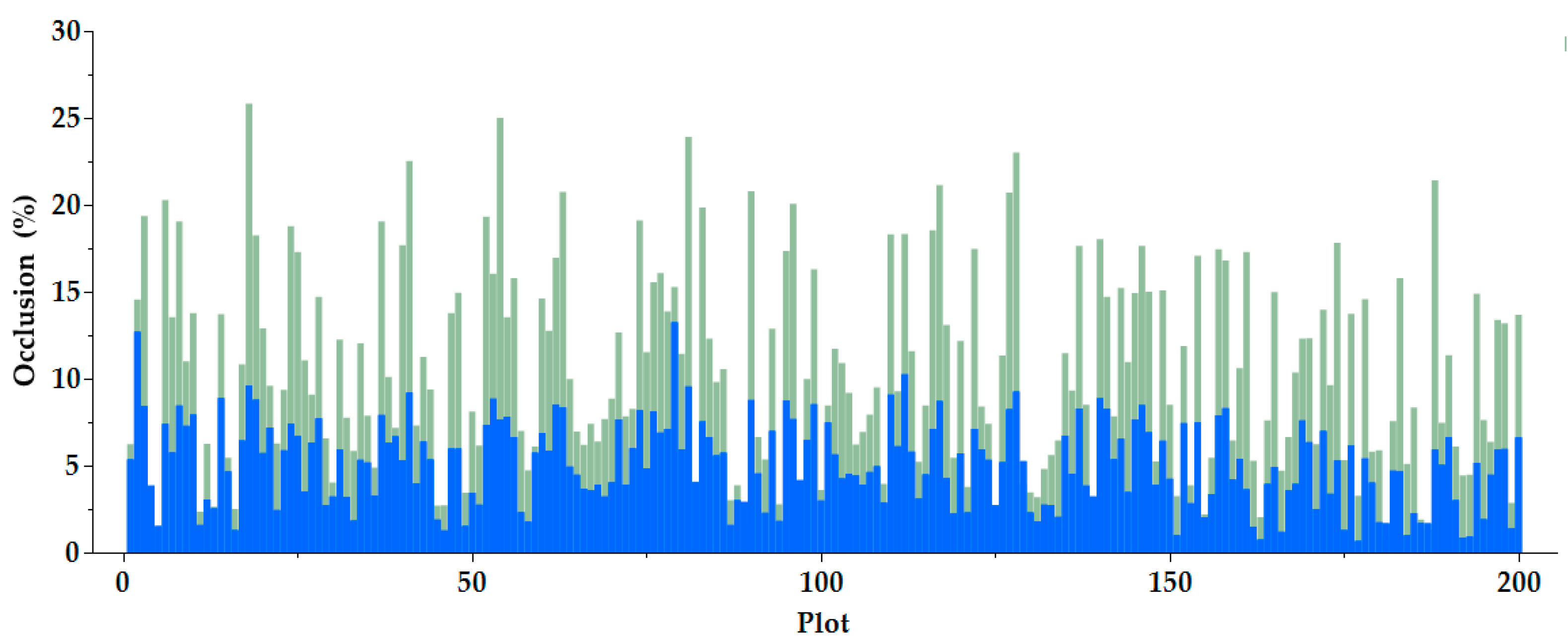
| Descriptive Statistic | Middle Scan Only | All Scans |
|---|---|---|
| Minimum | 0.84% | 0.68% |
| Maximum | 25.84% | 13.26% |
| Mean | 10.53% | 5.14% |
| Variance | 33.21% | 6.15% |
| Standard deviation | 5.76% | 2.48% |
Disclaimer/Publisher’s Note: The statements, opinions and data contained in all publications are solely those of the individual author(s) and contributor(s) and not of MDPI and/or the editor(s). MDPI and/or the editor(s) disclaim responsibility for any injury to people or property resulting from any ideas, methods, instructions or products referred to in the content. |
© 2023 by the authors. Licensee MDPI, Basel, Switzerland. This article is an open access article distributed under the terms and conditions of the Creative Commons Attribution (CC BY) license (https://creativecommons.org/licenses/by/4.0/).
Share and Cite
Bester, M.S.; Maxwell, A.E.; Nealey, I.; Gallagher, M.R.; Skowronski, N.S.; McNeil, B.E. Synthetic Forest Stands and Point Clouds for Model Selection and Feature Space Comparison. Remote Sens. 2023, 15, 4407. https://doi.org/10.3390/rs15184407
Bester MS, Maxwell AE, Nealey I, Gallagher MR, Skowronski NS, McNeil BE. Synthetic Forest Stands and Point Clouds for Model Selection and Feature Space Comparison. Remote Sensing. 2023; 15(18):4407. https://doi.org/10.3390/rs15184407
Chicago/Turabian StyleBester, Michelle S., Aaron E. Maxwell, Isaac Nealey, Michael R. Gallagher, Nicholas S. Skowronski, and Brenden E. McNeil. 2023. "Synthetic Forest Stands and Point Clouds for Model Selection and Feature Space Comparison" Remote Sensing 15, no. 18: 4407. https://doi.org/10.3390/rs15184407
APA StyleBester, M. S., Maxwell, A. E., Nealey, I., Gallagher, M. R., Skowronski, N. S., & McNeil, B. E. (2023). Synthetic Forest Stands and Point Clouds for Model Selection and Feature Space Comparison. Remote Sensing, 15(18), 4407. https://doi.org/10.3390/rs15184407