Monitoring Agricultural Land and Land Cover Change from 2001–2021 of the Chi River Basin, Thailand Using Multi-Temporal Landsat Data Based on Google Earth Engine

Abstract

In recent years, climate change has greatly affected agricultural activity, sustainability and production, making it difficult to conduct crop management and food security assessment. As a consequence, significant changes in agricultural land and land cover (LC) have occurred, mostly due to the introduction of new agricultural practices, techniques and crops. Earth Observation (EO) data, cloud-computing platforms and powerful machine learning methods can certainly support analysis within the agricultural context. Therefore, accurate and updated agricultural land and LC maps can be useful to derive valuable information for land change monitoring, trend planning, decision-making and sustainable land management. In this context, this study aims at monitoring temporal and spatial changes between 2001 and 2021 (with a four 5-year periods) within the Chi River Basin (NE–Thailand). Specifically, all available Landsat archives and the random forest (RF) classifier were jointly involved within the Google Earth Engine (GEE) platform in order to: (i) generate five different crop type maps (focusing on rice, cassava, para rubber and sugarcane classes), and (ii) monitoring the agricultural land transitions over time. For each crop map, a confusion matrix and the correspondent accuracy were computed and tested according to a validation dataset. In particular, an overall accuracy > 88% was found in all of the resulting five crop maps (for the years 2001, 2006, 2011, 2016 and 2021). Subsequently the agricultural land transitions were analyzed, and a total of 18,957 km² were found as changed (54.5% of the area) within the 20 years (2001–2021). In particular, an increase in cassava and para rubber areas were found at the disadvantage of rice fields, probably due to two different key drivers taken over time: the agricultural policy and staple price. Finally, it is worth highlighting that such results turn out to be decisive in a challenging agricultural environment such as the Thai one. In particular, the high accuracy of the five derived crop type maps can be useful to provide spatial consistency and reliable information to support local sustainable agriculture land management, decisions of policymakers and many stakeholders.

1. Introduction

Anthropogenic activities, such as Land Use (LU) and Land Cover (LC) changes, are affecting environmental conditions around the world, especially in developing countries [1,2]. In particular, LU/LC dynamics that involve deforestation and urban expansion boost carbon levels in the atmosphere and worsen climate change [3]. As a result, assessing LU/LC change could potentially offer several advantages concerning sustainable land use and key important drivers in the present and future [2,4]. According to SDGs (Sustainable Development Goals), Earth Observation (EO) data is a reliable source of information for mapping and monitoring agricultural land. Specifically, it provides valuable and reliable information for economic, social and environmental policies to accommodate LU/LC dynamics caused by population growth, suburbanization and agricultural expansion [5,6,7]. Fast progress in remote sensing technology provides a wide spatial distribution and, consequently, enables LU/LC monitoring and mapping over time [8].

Thailand is one of the main agricultural product exporters in the world. The country’s agricultural production has significantly contributed to domestic and global market demand, and as a consequence, agricultural activities have become a significant source of economic growth in the past decades [9]. The amount of cultivated area in 2020 was 23.88 billion hectares (about the 46.54% of the nation areas). The northeast region of Thailand is mainly suited to agriculture, and is actually the most highly cultivated area within the country (about 60% characterized by crop plantations). Many small landowners are located in this area and the agricultural business based on rice, cassava, sugarcane and para rubber (the main local crops) represents their main economic activity. Within this context, the Thai government has supported crop cultivation to increase areas and production for market demand, resulting in higher incomes for farmers [10,11].

Moreover, it is well know that farmers in the northeast region have acquired high adaptability to unfavorable conditions by using different crop management activities, many materials and national policies to increase productivity and production on the one hand, while still leading to intensive planting on the other hand [12,13]. Thus, this region is an important area for sustainable agricultural land management.

Although the northeast region of Thailand has the greatest agricultural areas and production in the country, increasing demands of agricultural production and renewable energy, as well as national policy, have recently influenced LU/LC patterns [11,13,14]. Specifically, forest and rice-growing areas have been replaced by other crops. With this premise, several main challenges have arisen including: crop management, food security, low productivity, lack of labor and irrigation management. Related agencies have started to work on these aspects; however, some of them are still present [15,16].

Remote sensing technology has evolved into a cutting-edge tool for merging multi-source images for high spatiotemporal resolutions for agricultural activity monitoring. EO data have been extensively utilized for mapping and monitoring agricultural crop fields from a variety of perspectives, including crop type, area of coverage, crop calendar, and yield, in different time periods [17,18,19]. At the same time, new technologies and EO data cloud platforms have enabled vast data computations by providing great opportunities for mapping land use on a large scale. For instance, the Google Earth Engine (GEE) is increasingly used across borders, mostly for agricultural area mapping [20]. As a result, EO data cloud computing platforms and powerful machine learning methods have undoubtedly improved analysis within the agricultural sector. Moreover, they provide free and open access information for all communities, which is very important in a sector such as this one, which is frequently characterized by climatic and environmentally related difficulties [21,22,23]. The information acquired by EO can subsequently serve as input data for numerous models that monitor changes in many natural resources, as well as predict significant scenarios such as natural disasters and crop type dynamics, including the changes of LC/LU consequences [17].

Several studies have highlighted that multi-temporal dataset combinations (i.e., Sentinel-1 (S1), Sentinel-2 (S2), and Landsat 8 (L8)) from multiple sensor sources, coupled with powerful machine learning approaches and time periods, make it possible to obtain crop classifications with high overall accuracy (OA > 85%) [11,24,25,26]. In particular, Som-ard, et al. [11] classified 13 different crop type classes in the Udon Thani province (Thailand) using the random forest (RF) algorithm, with OA > 87%, whereas Kluger, et al. [24] developed a procedure to map different crop shifts in France and Kenya using the RF classifier, achieving OA > 85%. Sun, et al. [25] identified three crop classes in the Yangzi River (China) using support vector machine (SVM), artificial neural network (ANN) and RF classifiers and showed up to 93% OA results. Tariq, et al. [26] classified five crop types in the Gujranwala District of Punjab Province, Pakistan from Decision-Tree-Classifier (DTC) and RF algorithms, and indicated OA values of > 85%. As highlighted in the previously reported studies, the efficiency of using multi-temporal data from multi-sensor data for classifying agricultural land/LC was proved. Moreover, they have shown that the RF classifier has the greatest efficiency and excellent results in terms of crop type/LC classification. However, a multi-temporal Landsat dataset for mapping several crop types for small field sizes—such as in Thailand—based on the RF algorithm is still a challenge.

Monitoring agricultural land dynamics using EO data over time makes it possible to offer valuable information on food management, related stockholders and environmental conditions [11,27]. Consequently, reliable and accurate information of cropland/LC maps at the national or international levels can be obtained. Such information can be subsequently involved in many applicable problems in agricultural lands and LC change monitoring. However, mapping, monitoring and evaluating crop/LC types in small areas (i.e., field < 1 ha sizes) and complicated landscapes is still a real problem, especially when areas are regularly characterized by high cloud cover, such as in Thailand.

Within this framework, in this work, proper mapping and monitoring of temporal and spatial dynamics related to LU/LC was performed in the northeast Thailand area within five different years from 2001 to 2021 (2001, 2006, 2011, 2016, and 2021). In particular, all available Landsat archives were involved inside the Google Earth Engine (GEE) platform, making it possible to produce several LU/LC maps for each period by adopting an RF classifier. Therefore, different sophisticated classification approaches without even downloading the satellite dataset were adopted in order to achieve the highest map accuracy of our result.

It is important to highlight that in this work, cutting-edge methods and technology, such as remote sensing and a machine learning technique, were adopted. In particular, in this work, the main aims were to: (i) produce LC maps focusing on the main local crops (i.e., rice, cassava, para rubber, and sugarcane crops) within the Chi River Basin in (NE-Thailand); (ii) monitor long-term transitions in agricultural land and LC transformations within four 5-year periods (2001–2006, 2006–2011, 2011–2016, and 2016–2021).

The main advantages of this work are to use reliable historical agricultural land and LC to substitute ground truth and training samples in satellite images. Resulting map accuracy and reliability can be attributed to two distinct key drivers: agricultural policy and staple prices. Therefore, all this information can be useful to support sustainable agriculture land organization, food management, decisions of government and many agricultural industries.

2. Study Area and Materials

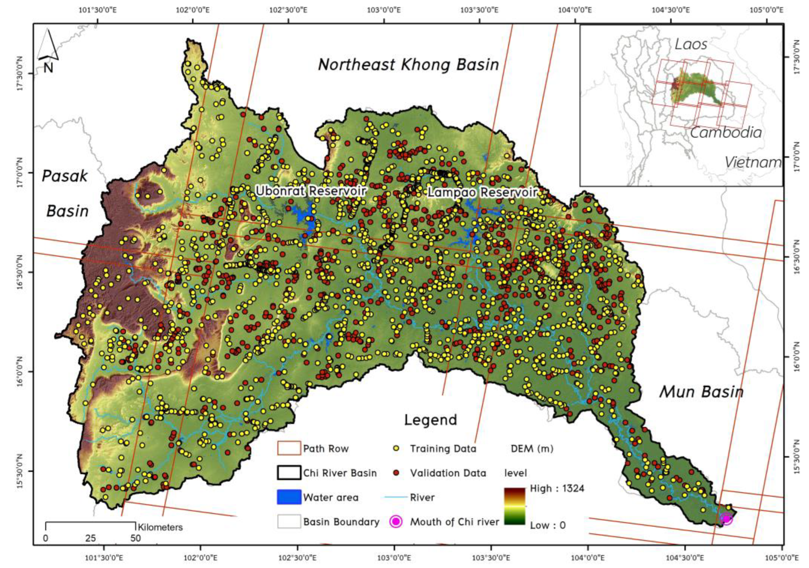
In this work, multi-temporal Landsat image data (i.e., L5, L7, L8 and L9), as well as local and auxiliary geo-data, were jointly used in order to map and monitor four time periods of agricultural land dynamics in Thailand. In particular, the salient points can be summarized as: (i) preprocessing and feature extraction of the Landsat data; (ii) crop type/LC classification by the RF algorithm; (iii) crop type/LC map generation and evaluation of agricultural land changes over a 20-year period. A workflow containing all steps involved in the work are reported in Figure 1.

2.1. Study Area

The study area is located in the Chi River Basin (NE-Thailand) and is characterized by having agriculture cultivations for almost ⅔ of the land use. In particular, the dominant crops are: rice, sugarcane, para rubber and cassava [28]. The Chi River Basin covers an area of 49,132 km², accounting for 29% of this region (between 15°10′ to 17°50′N and 101°00′ to 105°50′E) (Figure 2). The Chi River Basin is characterized by having plains and highlands topographical features, and the height above mean sea level differs from 0 to 1324 m. In particular, the central and western parts of this region are part of the Dong Phayayen Mountains, a place known as the starting point for the Chi river and several tributaries such as Nam Phong, Lam Pao and Nam Yang. All of these tributaries are very important for local agricultural cultivations and livelihoods since they represent the water sources of the area. From a climatic standpoint, the study region is classified as tropical semi-humid wet/dry-savanna (Köppen climate, classification: Aw), characterized by high cloudiness and inclement weather, as well as three different seasons of summer, rainy, and winter, ranging from February to May, May to October, and October to February, respectively. Finally, considering temperature, the long-term temperature (average 10 years) is about 27 °C and the average annual precipitations are about 1690 mm. The relative humidity in this region is approximately 72% [29].

2.2. Reference Data

Approximately 3290 sampling points (SP) were randomly collected within the Chi River Basin and used as reference data in order to train and validate the RF classifier approach. Subsequently, SP was randomly spilt in two different datasets in order to obtain the training and validation sets involved in the RF classification algorithm. In particular, 2303 (70%) sampling points were used for the training phase and 987 (30%) for the validation phase (Figure 2). Within SP, eight different major classes were collected, as reported in

Table 1. Reference data sets of crop type/LC over Chi River Basin, Thailand in years 2001, 2006, 2011 and 2021.

Crop Type/LC	2001		2006		2011		2016		2021
	Color Orthophoto		Google Earth Pro						Field Campaigns
	Training	Validation	Training	Validation	Training	Validation	Training	Validation	Training	Validation
Rice	261	112	341	146	335	144	301	129	340	146
Sugarcane	890	381	836	358	742	318	615	264	452	194
Cassava	61	26	63	27	180	77	235	101	240	103
Para rubber	247	106	227	97	209	90	311	133	365	156
Built-up	350	150	350	150	350	150	350	150	350	150
Forest	303	130	272	117	268	115	243	104	225	96
Water	118	51	126	54	125	54	136	58	150	64
Bare soil	73	31	88	38	94	40	112	48	181	78
Total	2303	987	2303	987	2303	987	2303	987	2303	987

, including rice, sugarcane, cassava, para rubber, forest, built-up, water and bare soil. It is worth highlighting that SP field campaigns were performed between May and July 2021. Consequently, different methods aimed at collecting reference data were involved in this work in order to construct and validate the five classifications corresponding to the 2001, 2006, 2011, 2016 and 2021 years. Details on how the reference data were acquired for the different years considered in this work are given below.

• 2021 year: A total of 3290 sampling points were collected as reference data from a field survey performed between 15 May 2021 and 30 July 2021. Point position was then georeferenced with high accuracy by a handheld Global Positioning System (GPS) version Garmin 62 s [30].
• 2006, 2011 and 2016 years: The same 3290 sampling points considered in the 2021 year were photo-interpreted and digitized using very high-resolution data available within the Google Earth pro imagery database.
• 2001 year: In addition, the same reference points were photo-interpreted, digitized and finally acquired through very high-resolution color orthophoto images provided by the Land Development Department (LDD) [11]. LDD color orthophoto images were used to search and record different agricultural land fields/LC within the Chi River Basin. LDD is characterized by having spatial resolution equal to 1 m. Moreover, to improve sampling point dataset reliability, authors interviewed 20 local farmers who have been farming and living for over 20 years in the area.

2.3. Landsat Image Datasets

This study involved a total of 428 Landsat images in order to map the crop type/LC within the Chi River Basin. In particular, L5, L7, L8 and L9 Level-2 products (atmospherically corrected) were used in this work, and 78, 78, 48, 90 and 134 Landsat scenes were used for the 2001, 2011, 2016 and 2021 base years, respectively. Specific information about the Landsat mission and the corresponding number of images involved are reported in

Table 2. Landsat image datasets deployed for mapping agricultural fields/LC in 2001, 2006, 2011, 2016 and 2021. The number of scenes show the availability for crop type/LC mapping. Landsat-5 (L5) images were applied for 2001, 2006 and 2011, and Landsat-7 (L7) data was adapted in analysis for only 2001. Landsat-8 (L8) images were employed for mapping in years 2016 and 2021, while Landsat-9 (L9) datasets were included for 2021.

Image Data (January–December)	Sensor	Years (Scenes)
		2001	2006	2011	2016	2021
Landsat-5	TM	45	78	48
Landsat-7	ETM+	33
Landsat-8	OLI				90	112
Landsat-9	OLI-2					22
Total (scenes)		78	78	48	90	134

. Through the GEE platform, only the scenes characterized by having less than 30% cloud cover were selected.

It is worth reminding that the L5 and L7 images are characterized by having seven and eight portions of spectral information, respectively, while a total of eleven bands, with a spatial resolution of 30 m, are present in the L8 and L9 data [31,32]. Despite the fact that several bands are available within the Landsat data, in this work, only six bands were involved. In particular, blue: 490 nm, green: 560 nm, red: 665 nm, NIR: 842 nm, SWIR1: 1910 nm and SWIR2: 2190 nm bands were used. These six pieces spectral information are known in the literature due to the possibility to produce several vegetation indices (VIs) able to detect, monitor and map different crop types [11].

Land surface can be labelled with VIs that are able to identify and monitor phenological crop dynamics [33]. The main aims include crop type and LC classification [13,34]. In this study, according to

Table A1. Nine vegetation indices (VIs) for crop type and LC classification for five base years.

Indices	Abbreviation	Formula	Reference
Normalized Difference Vegetation Index	NDVI	$\mathrm{NDVI}=\frac{\mathrm{NIR}-\mathrm{red}}{\mathrm{NIR}+\mathrm{red}}$	Rouse [58]
Maximum NDVI	maxNDVI	$\mathrm{maxNDVI}=\max \{\mathrm{NDVI}{(\mathrm{i},\mathrm{j})}_1,\mathrm{NDVI}{(\mathrm{i},\mathrm{j})}_2,\mathrm{\dots },\mathrm{NDVI}{(\mathrm{i},\mathrm{j})}_n\}$	Cihlar, et al. [59]
Minimum NDVI	minNDVI	$\mathrm{minNDVI}=\min \{\mathrm{NDVI}{(\mathrm{i},\mathrm{j})}_1,\mathrm{NDVI}{(\mathrm{i},\mathrm{j})}_2,\mathrm{\dots },\mathrm{NDVI}{(\mathrm{i},\mathrm{j})}_n\}$
Enhance Vegetation Index	EVI	$\mathrm{EVI}=\mathrm{G}\times \frac{\mathrm{NIR}-\mathrm{red}}{\mathrm{NIR}+\left(C_1\times \mathrm{red}\right)-\left(C_2\times \mathrm{B}\right)+\mathrm{L}}$	Huete, et al. [60]
Normalized Difference Water Index	NDWI	$\mathrm{NDWI}=\frac{\mathrm{GREEN}-\mathrm{NIR}}{\mathrm{GREEN}+\mathrm{NIR}}$	McFeeters [61]
Soil-Adjusted Vegetation Index	SAVI	$\mathrm{SAVI}=\frac{\mathrm{NIR}-\mathrm{red}}{\mathrm{NIR}+\mathrm{red}+\mathrm{L}}\left(1+\mathrm{L}\right)$	Huete [62]
Ratio Vegetation Index	RVI	$\mathrm{RVI}=\frac{\mathrm{NIR}}{\mathrm{red}}$	Jordan [63]
Normalized Difference Infrared Index	NDII	$\mathrm{NDII}=\frac{\left(\mathrm{NIR}-\mathrm{SWIR}1\right)}{\left(\mathrm{NIR}+\mathrm{SWIR}1\right)}$	Hardisky [64]
Normalized difference moisture Index	NDMI	$\mathrm{NDMI}=\frac{\left(\mathrm{NIR}-\mathrm{SWIR}2\right)}{\left(\mathrm{NIR}+\mathrm{SWIR}2\right)}$	Gao [65]

, nine different potential VIs were selected among the main ones present in the literature in order to separate crop type classes.

As mentioned in the previous section, the Chi River Basin is characterized by high cloudiness and inclement weather. Therefore, a median composite (MC) was applied to initiate gap-free image composites that are spatio-temporally consistent.

According to previous studies [35,36], the MC algorithms can provide consistent phenological datasets and reduce cloud conditions over large coverage regions with the requirement of an atmospheric correction and accurate cloud masking [34,37].

MC was applied to all spectral bands and the derived VIs were involved in this work. Composites were implemented for all years and for all time steps considered in this work. Specifically, Landsat data available from January to December of each year were collected and MC was subsequently computed in order to generate a single annual image for each VI considered for each of the five years (i.e., 2001, 2006, 2011, 2016 and 2021). In particular, MCs composites were generated by using the “ee.Reducer.median()” and mosaicked by the “ee.Reducer.mosaic()” function available on GEE. The resulting images were finally compared with high-resolution imagery available in Google Earth Pro in order to assess their output quality.

Final number of annual image composites (i.e., spectral bands and derived VIs) and topographical indicators used for mapping agricultural fields/LC for each of the five base years are reported in

Table 3. All features (i.e., the spectral bands, vegetation indices (VIs) and topographical variables) were used for agricultural fields/LC classification in 2001, 2006, 2011, 2016 and 2021.

Feature Data	2001	2006	2011	2016	2021
	L5 & L7	L5	L5	L8	L8 & L9
Spectral bands	12	6	6	6	12
Vegetation indices (VIs)	18	9	9	9	18
Topographic	2	2	2	2	2
Total (Full Set of Features)	32	17	17	17	32

.

2.4. Auxiliary Geo-Data

Related geo-data can offer significant information to support disentangling different crop phenology and other specific agricultural practices [38]. For this reason, the digital elevation model (DEM) dataset was involved in this work in order to retrieve elevation and slope variables. DEM was obtained for free from the Land Processes Distributed Active Archive Center (LP DAAC) (United States) at 30 m of spatial resolution [39].

3. Methods

3.1. Supervised Classification

In agriculture, the RF algorithm is commonly used for classification and regression problems [40]. This classifier is a decision tree (DT)-based ensemble machine learning classifier. The bootstrap with replacement technique generates multiple sample data sets and, as a result, individual and independent DTs, the results of which are combined for the majority decision [40]. The expected generalization error based on “out-of-bag” (OOB) data is considered as one of the primary advantages derived from the RF algorithm. Other advantages include the internal relevance measure of the input features and the ability to adapt to a large number of input features. Many previous studies have demonstrated the high efficiency of feature importance in selecting the most relevant variables for crop type/LC classification in order to minimize over-fitting, and for well-organized computations [25,41,42,43].

For this research, the “Mean Decrease in Accuracy” (MDA) measure was employed for a recursion feature selection, as in earlier studies [11,44,45]. It should be noted that the derived feature significance was calculated in R version 4.2.2 using the random forest package [46].

The RF classification model requires two hyper-parameters, which are the number of randomly nominated features for each node (mtry) and the number of trees (ntree). In particular, we implemented ntree setting from 50 up to 1500 with the default of the mtry (the square root of the total number of input variables). Subsequently, we selected the best parameter as 1000 trees based on the OOB result for all five base years.

Based on the 2303 sampling points, RF models were trained to categorize eight crop type/LC classes for each of the five base years (Table 1). The feature variables, comprising spectral bands, derived VIs, and supplementary geo-data, were used for all time steps. Appendix A lists the top ten most important features for each year (details in

Table A2. Ranking features the importance of the top 10 variable sets from the random forest (RF) models in 2001, 2006, 2011, 2016 and 2021.

Time Periods	Feature Variables
2021	maxNDVI_L8, SWIR2_L9, EVI_L8, SWIR1_L9, NIR_L8, SWIR1_L8, SAVI_L8, Green_L9, EVI_L9, minNDVI_L9
2016	NIR_L8, maxNDVI_L8, EVI_L8, SWIR1_L8, SAVI_L8, Green_L8, NDWI_L8, SWIR2_L8, Red_L8, NDII_L8
2011	maxNDVI_L5, SWIR2_L5, SWIR1_L5, EVI_L5, NIR_L5, RVI_L5, SAVI_L5, Red_L5, Green_L5, NDVI_L5
2006	maxNDVI_L5, EVI_L5, SWIR1_L5, Blue_L5, NIR_L5, SWIR2_L5, SAVI_L5, Green_L5, NDVI_L5, RVI_L5
2001	NDWI_L5, NDVI_L5, SWIR1_L5, maxNDVI_L7, SWIR_L7, NIR_L7, Red_L7, RVI_L5, maxNDVI_L5, EVI_L7

).

The MDA and OOB findings for the five base years were examined for evaluating the efficiency of the optimized RF classification models, and the final RF models were evaluated from the independent data set using the GEE and utilized to predict the entire data set.

3.2. Accuracy Evalutation

The accuracy assessment of the results of this work was conducted consisting of two parts:

• The generalization error provided by the OOB result was utilized to assess the effectiveness of the RF classifier [40,46].
• The accuracy of the crop type/LC maps was generated using an independent validation dataset (987 reference points). As mentioned previously, the validation dataset was collected from a field survey for 2021 and from visual interpretation by using very high-resolution data available within the Google Earth pro imagery for 2001, 2006 and 2011 (Table 1). The maps’ accuracy evaluations were assessed by combining typical statistics resulting from the confusion matrix, such as overall accuracy (OA), user’s accuracy (UA), producer’s accuracy (PA) [47] and the kappa statistic [48].

Furthermore, the uncertainty of area estimations was examined for each year based on the related 95% confidence interval. Finally, the rates of classification errors enabled in modifying of crop type/LC map estimated areas using the stratified evaluation approach was proposed by Olofsson, et al. [49].

3.3. Post-Classification

In order to assess the crop types/LC maps variability over time, the five base year maps were investigated. Specifically, a post-classification comparison method was applied at pixel level for the areas that have transformed “from to” over time. This analysis made it possible to monitor and map how crop type areas transformed over the four time periods (i.e., 2001–2006, 2006–2011, 2011–2016 and 2016–2021). A chord diagram was used to show the temporal change of the different time periods. The chord diagram shows a set of nodes of proportional crop type/LC areas, and connected nodes demonstrate crop transitions from one to another for each time period.

4. Results

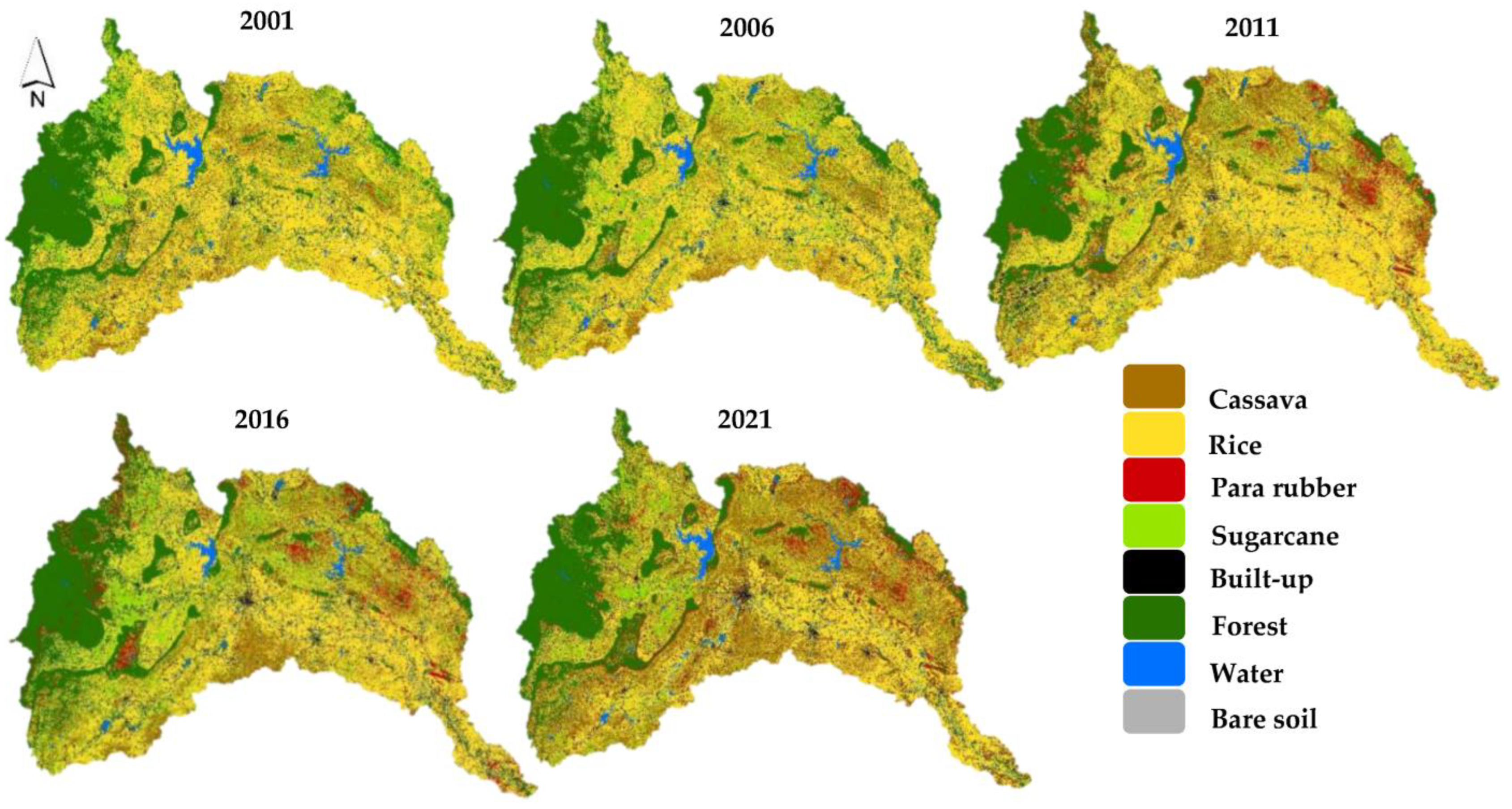
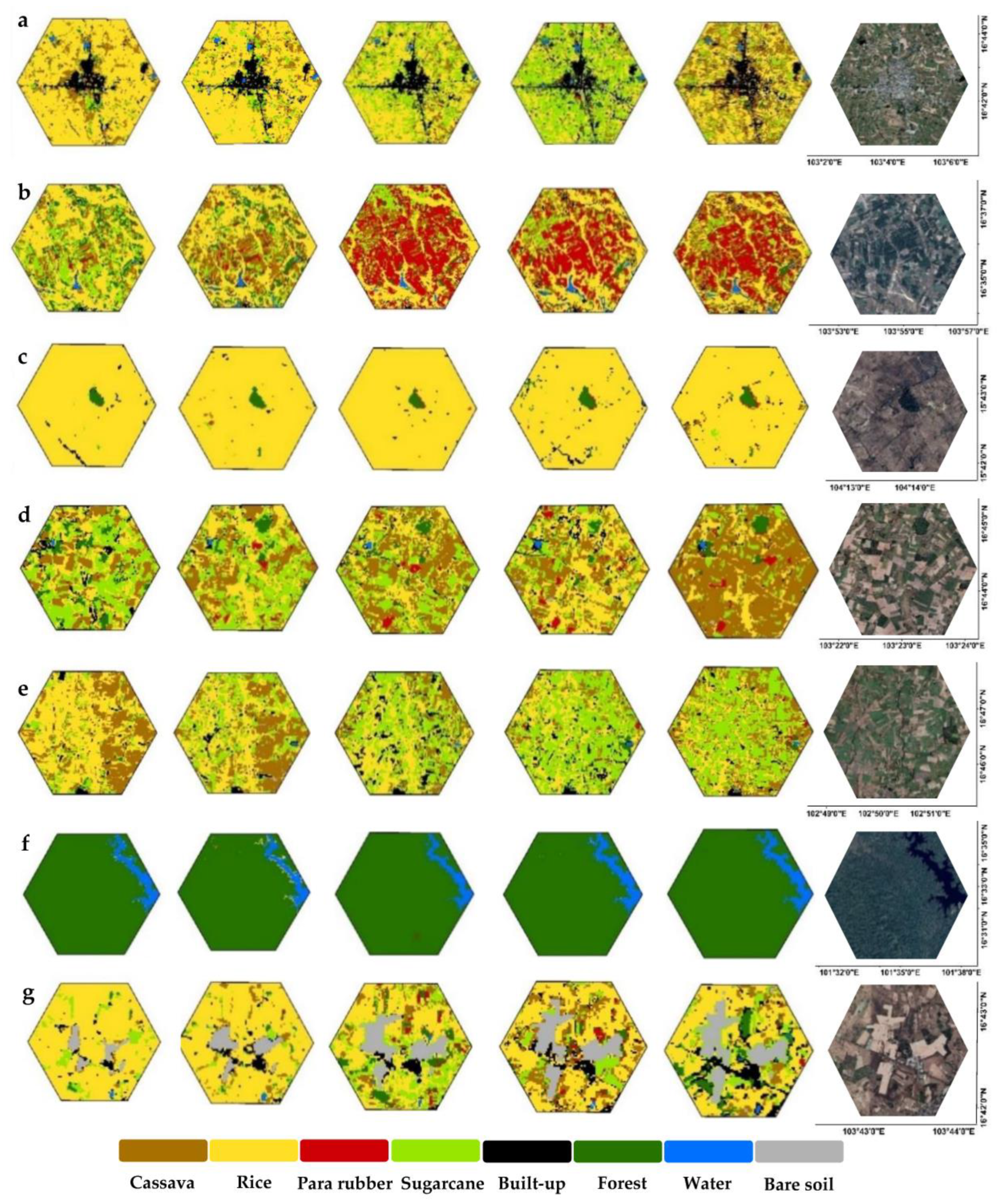
4.1. Crop Type/LC Classification

RF classification maps are reported in Figure 3. These maps turn out to be very useful to monitor LC dynamics over time; thus, it can be noted that some classes have changed over the years while others have remained stable in terms of area. For example, on the 2001 map, the main classes are rice and forest; while considering the same classes in the 2021 map, they seem to have less impact. This assumption can actually be made, specifically when considering that the cassava class area within the 2001 map compared to the 2021 map rises from about 5000 km² to almost 12,000 km², respectively. Moreover, in addition to the cassava increase, para rubber, sugarcane and built-up land also register large surface increments. Specifically, during the observed period, there is an increase from dozens of km² to over 3000 km² for para rubber, from about 4500 km² to almost 6000 km² for sugarcane and from about 2000 km² to almost 3000 km² for built-up land, respectively, in the maps referring to 2001 and 2021. In contrast, rice cultivation, an opposite behavior, can be observed, i.e., a decline in rice fields cultivation over time. Specifically, fields classified as rice in 2001 covered about 25,000 km², while there was only 17,000 km² in 2021. In contrast, considering the water classes and bare soil, these have remained constant over time in terms of surface.

In order to better understand class variations over time, hexagon examples of crop types/land cover (LC) classifications considering the eight classes for the entire observed period within the Chi River Basin were reported (Figure 4). In particular, a qualitative increase in area is again observed over time in the cassava, para rubber, sugarcane and built-up land classes. Specifically, row d of Figure 4 shows a large change in comparisons of the cassava class between 2016 and 2021. In contrast, with regard to the hexagons representing the para rubber class (row b), a large change in LC can be observed between 2006 and 2011. The hexagons representing the sugarcane class (line b) show a large variation between 2001 and 2011, while the one representing the water class (row f) show no variation between the years. The interesting point that arises is that, according to Figure 4, LC variation does not occur between two specific periods, but can in relation to the class observed that can occur between different years.

Following the primary performance parameters that had been calculated (refer to the section in Materials and Methods for more information), a comparison and discussion of each classifier was proposed with reference to the validation set that was presented in Table 1. Results related to the model accuracy and validation were reported in Figure 5 and

Table 4. Accuracy assessment using independent validation datasets for eight crop type/land cover (LC) classification results in 2001, 2006 and 2011 from all available Landsat datasets and a random forest (RF) classifier. (OA: overall accuracy, PA: producer’s accuracy, UA: user’s accuracy).

2001 Crop Types	Reference Data
	Cassava	Rice	Para Rubber	Sugarcane	Built-Up	Forest	Water	Bare Soil	Total	UA (%)
Cassava	96	5	3	6	1	1	0	0	112	85.71
Rice	22	339	0	12	4	3	1	0	381	88.98
Para rubber	0	0	26	0	0	0	0	0	26	100.00
Sugarcane	10	5	0	88	0	3	0	0	106	83.02
Built-up	1	4	0	0	144	1	0	0	150	96.00
Forest	0	0	4	0	1	125	0	0	130	96.15
Water	0	3	0	0	2	3	43	0	51	84.31
Bare soil	0	0	0	0	0	0	0	31	31	100.00
Total	129	356	33	106	152	136	44	31	987
PA (%)	74.42	95.22	78.79	83.02	94.74	91.91	97.73	100.00
OA = 90.37%; Kappa = 87.80%
2006	Cassava	Rice	Para rubber	Sugarcane	Built-up	Forest	Water	Bare soil	Total	UA (%)
Cassava	114	12	0	20	0	0	0	0	146	78.08
Rice	25	319	1	7	4	2	0	0	358	89.11
Para rubber	0	0	25	0	0	2	0	0	27	92.59
Sugarcane	16	5	0	75	0	1	0	0	97	77.32
Built-up	0	0	0	1	147	0	0	2	150	98.00
Forest	0	2	1	1	0	113	0	0	117	96.58
Water	0	1	0	2	1	2	48	0	54	88.89
Bare soil	0	1	0	0	2	1	0	34	38	89.47
Total	155	340	27	106	154	121	48	36	987
PA (%)	73.55	93.82	92.59	70.75	95.45	93.39	100.00	94.44
OA = 88.65%; Kappa = 85.78%
2011	Cassava	Rice	Para rubber	Sugarcane	Built-up	Forest	Water	Bare soil	Total	UA (%)
Cassava	110	12	0	22	0	0	0	0	144	76.39
Rice	18	283	0	12	3	2	0	0	318	88.99
Para rubber	0	0	74	0	0	3	0	0	77	96.10
Sugarcane	16	3	0	71	0	0	0	0	90	78.89
Built-up land	0	0	0	0	148	0	0	2	150	98.67
Forest	0	1	2	1	0	110	0	0	114	96.49
Water	0	0	0	2	1	2	49	0	54	90.74
Bare soil	0	0	0	0	2	1	0	37	40	92.50
Total	144	299	76	108	154	118	49	39	987
PA (%)	76.39	94.65	97.37	65.74	96.10	93.22	100.00	94.87
OA = 89.36%; Kappa = 87.08%

and

Table 5. Accuracy assessment using independent validation datasets for eight crop type/land cover (LC) classification results in 2016 and 2021 based on all available Landsat datasets and a random forest (RF) classifier. (OA: overall accuracy, PA: producer’s accuracy, UA: user’s accuracy).

2016 Crop Types	Reference Data
	Cassava	Rice	Para Rubber	Sugarcane	Built-Up	Forest	Water	Bare soil	Total	UA (%)
Cassava	106	5	1	17	0	0	0	0	129	82.17
Rice	18	237	0	8	0	1	0	0	264	89.77
Para rubber	2	0	98	0	0	1	0	0	101	97.03
Sugarcane	16	4	2	111	0	0	0	0	133	83.46
Built-up	0	4	0	0	145	0	0	1	150	96.67
Forest	0	3	0	0	0	101	0	0	104	97.12
Water	0	6	0	2	3	2	45	0	58	77.59
Bare soil	0	1	0	1	0	0	0	46	48	95.83
Total	142	260	101	139	148	105	45	47	987
PA (%)	74.65	91.15	97.03	79.86	97.97	96.19	100.00	97.87
OA = 90.07%; Kappa = 88.21%
2021	Cassava	Rice	Para rubber	Sugarcane	Built-up	Forest	Water	Bare soil	Total	UA (%)
Cassava	119	3	3	16	0	5	0	0	146	81.51
Rice	3	185	0	4	1	0	0	1	194	95.36
Para rubber	0	0	98	0	0	5	0	0	103	95.15
Sugarcane	18	2	0	136	0	0	0	0	156	87.18
Built-up	0	2	0	0	147	0	0	1	150	98.00
Forest	0	0	2	0	0	94	0	0	96	97.92
Water	0	1	0	0	0	3	60	0	64	93.75
Bare soil	0	0	0	0	0	0	0	78	78	100.00
Total	140	193	103	156	148	107	60	80	987
PA (%)	85.00	95.85	95.15	87.18	99.32	87.85	100.00	97.50
OA = 92.91%; Kappa = 91.76%

.

Considering Figure 5, the average values of OA (model accuracy), Kappa (model accuracy), OA (validation) and Kappa (validation) are 86.7%, 83.4%, 90.3% and 88.1%, respectively. Such high average values of OA and Kappa validation confirm the goodness of the proposed classifications. However, considering OA over the years, the 2021 results have the highest values (OA = 92.9%), while 2006 results have the lowest (OA = 88.7%).

Considering PA and UA, they were generated starting from independent validation datasets (Table 1) for eight crop types/LC over the five time steps and are reported in Table 4 and Table 5. The classification map in 2021 achieved height accuracy with OA and kappa of 92.9% and 91.8%, while other map results obtained accuracies > 85%.

For classification results in 2001, 2006, 2011 and 2016, almost all crop types/LC had PAs and UAs with accuracies higher > 75%. The greatest misclassifications were obtained in the classes of “cassava” and “sugarcane”. Mapping agricultural land or LC in 2021 achieved accuracies > 90% for nearly all classes. Conversely, the class of cassava achieved the highest confusion with ≤ 85%.

Figure 6 provides a visual representation of the mapped and estimated areas of the various crop type classes in the Chi River Basin for each of the five periods, along with the confidence intervals (CI) for 95% of the data. In our results, in 2001, 2006, 2011, 2016 and 2021, small differences appeared between mapped and estimated areas, as shown by the 95% CI of the error bars.

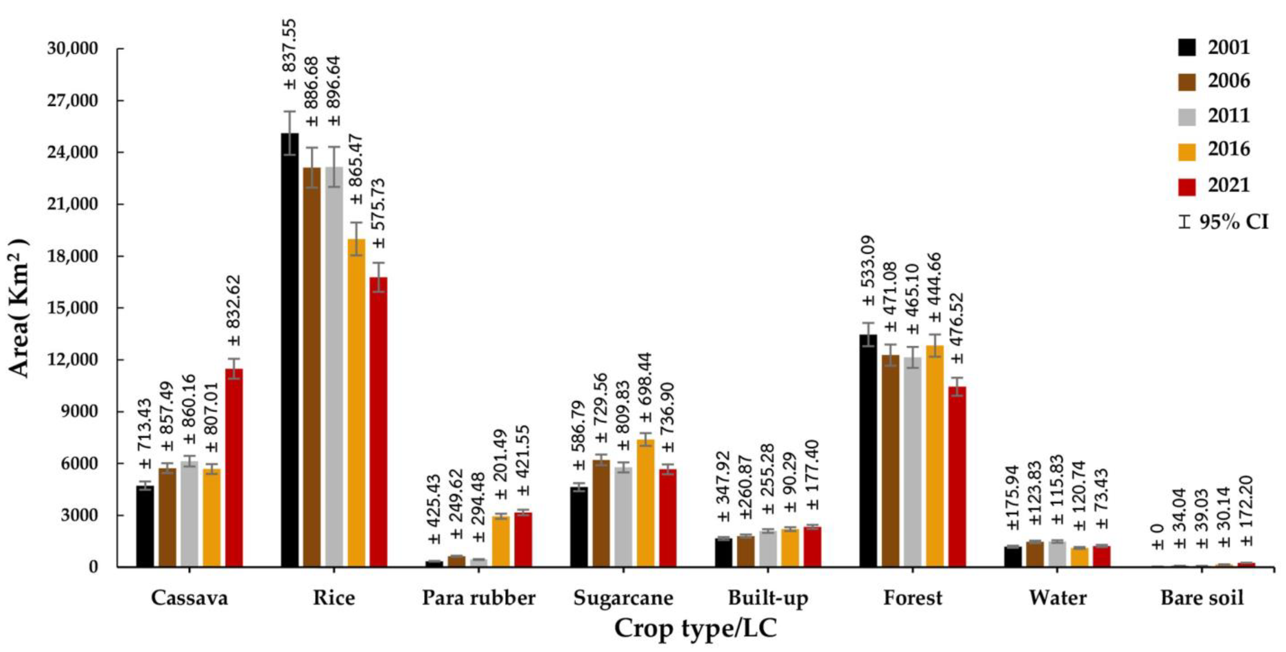
4.2. Crop Type Dynamics

The main factors driving crop type transition have been highlighted via an analysis of classification maps and crop type changes in five time periods (Figure 7). The highest crop type transformation occurred for a recent period between 2016 and 2021 of 9966 km², followed by 2011 to 2016 (8740 km²), 2001 to 2006 (4876 km²) and 2006 to 2011 (1068 km²). Between 2001 and 2006, the crop transition with the greatest increase in terms of area can be related to sugarcane (1579 km²) and cassava (1009 km²). However, this increase resulted in a reduction in rice cultivation of 1993 km². The largest percentage increases in areas under cultivation have been observed for cassava (405 km²) and rice (39 km²) between the years 2006 and 2011. In contrast, a decrease in crop area was seen in sugarcane, which covered 438 km². Between the years 2011 and 2016, the crop areas that have the potential to generate the highest increase in yield are sugarcane (1615 km²) and para rubber (2502 km²). In contrast, rice areas dropped by 4169 km². From 2016 to 2021, the areas of major crops expanded, in particular for cassava (5804 km²) and para rubber (220 km²). In contrast, rice areas decreased to a total of 2217 km² due to encouragement from the government’s policy for changing crop cultivation in northeast Thailand. Moreover, Figure 7 illustrates the crop type area transition for the four five-year periods, highlighted in the chord diagrams. From 2001 to 2006, the highest crop type transition was from rice to cassava. From 2006 to 2011 and 2011 to 2016, the same changes occurred in the major crop types, from rice to sugarcane. The largest change from rice to cassava-cultivated areas was observed between 2016–2021.

5. Discussion

5.1. Crop Type/LC Classification Assessment

The joint use of optimized RF classification models (involving single bands and VIs) and auxiliary geo-data presented results of agricultural fields/LC classifications. As reported in Figure 5, the constructed RF classification models achieved excellent results in all five time periods analyzed. Specifically, the highest accuracy of the crop type/LC classification has been observed in 2021, followed by 2001, 2016 and 2006, respectively. Specifically, 2021 accuracy is always higher than in other years, which can certainly be related to the number of images available for the year in question (134 scenes available in the 2021 compared to 40/90 available in other years). The efficient result of 2021 that used the high spectral and temporal information of the combined analysis of Landsat data sets (i.e., L8 and L9) as well as the availability of high-quality ground-truth data were used. Recent studies [11,27] also highlighted the multi-temporal Landsat data support LC and crop type classifications. Furthermore, implementing important RF feature rankings makes it possible to select the input variables when applying the classification to large-scale mapping. Similar results were reported by Pflugmacher, et al. [38], who highlighted the efficiency for use in automated mapping of crop type/LC in the large region using Landsat spectral-temporal metrics. In our study, Landsat spectral-temporal compositing, together with the powerful RF classifier, showed very good results for crop type/LC mapping when dealing with a wide scale and cloudy region.

In 2006, 2011 and 2016, high PAs and UAs were obtained in almost all specific classes. Conversely, the highest commission was obtained in 2006 between rice and cassava and also sugarcane and cassava due to the similar spectral information based on crop phenology, leading to misclassification. In 2011, the highest misclassification occurred between sugarcane and cassava, as well as rice and cassava, probably due to spectral signatures overlapping. Meanwhile, in 2016, the most significant crop confusion was between rice and cassava and also cassava and sugarcane because several sugarcane and cassava fields were recently cultivated during this time, leading to similar signatures, as seen in previous findings [13].

Combining both Landsat sensor datasets for 2001 (L5 and L7) and 2021 (L8 and L9) was a good strategy to support crop separation, which consequently led to better classification results for nearly all classes involved in this work. The aggregated Landsat sensor datasets for 2001 demonstrated high efficiency for mapping crop types and LC. The confusion was shown between rice and cassava and also between rice and sugarcane due to rice crop phenology in the reproduction phase being similar in some cassava and sugarcane fields, leading to the loss of accuracy in the results. For 2021, the map result was smoothed well and reduced noises in crop type areas. Nevertheless, the commission between sugarcane and cassava still persists because sugarcane crop phenology in tillering and grand growth stages are similar to cassava canopy, leading to mixed spectral signatures, as reported by Som-Ard, et al. [50]. In addition, cassava within the Chi River Basin is usually planted in all seasons; therefore, the canopy and greenness are similar compared to the vigor of sugarcane. In our study, this suggests increasing ground truth data for crop type classes across the study region.

The multi-temporal Landsat data and the RF classifier based on GEE produced very excellent results (OA above 85%) in this research. This is consistent with studies that show the utility of spectral and temporal data in monitoring crop types and land change [27,34,38,51]. Therefore, due to the high accuracy in crop classification mapping obtained in this work a transferability can be applied for monitoring different agricultural contexts in other regions or countries. Moreover, GEE generated good crop maps even if areas was characterized by having high rainfall and cloudy weather. However, for a national scale such Thailand, with high cloud cover and small field sizes (<1 ha) and complex landscapes, the GEE is still challenging due to several limitations (i.e., data availability, processing time, and potential inaccuracies). Future studies should consider these points for improving the accuracy of crop type map results.

Som-ard, et al. [11] in order to increase spectral and temporal information for crop type/LC mapping suggested to use Landsat-9 data. Specifically, they obtain outstanding results in the 2021 crop type classification in Udon Thani Province (Thailand). However, the constraint of this study was limited to cloud cover conditions, leading to image distortions of spectral reflectance.

Considering the variables useful to generate a crop classification map, in this work we highlight that maxNDVI variable result to be the most important feature able to reduce cloud coverage impacts (in Appendix A Table A2). Such result is consistent with the literature, in particular Griffiths, et al. [35], Li, et al. [52], Xu, et al. [53], Ghassemi, et al. [54], highlight that maxNDVI feature overcomes the cloudy impacts for regional to global crop type or LC classifications.

Considering crop types/LC classifications carried out in Thailand present in literature Emparanza, et al. [55] mapped four major classes (i.e., urban, crop, forest and water) in Thailand’s Eastern Economic Corridor (EEC) obtaining > 90% of OA using convolutional neural network (CNN) and satellite images. Kruasilp, et al. [56] classified LC (six classes including agricultural land, built-up area, forest, para rubber, maize, and water) using the RF classifier and multiple satellite data (S1, S2 and Landsat data) for Nan province (small region), obtaining an OA range between 52–97%. Daraneesrisuk, et al. [57] generated a crop classification map based on the RF algorithm by combining S1 and S2 data. In particular they focus their attention on sugarcane and cassava crop in a small area (Khon Kean province) and obtain an OA equal to 68%. However, in this last work the authors produced a few crop type classes and did not measure optimized-feature RF classification models for a large-scale mapping. Results obtained in this work appear to be very high in comparison to those mentioned above. Despite several crop mapped classes (eight crop type classes) excellent results were obtained by optimizing RF model and involving all available Landsat data in a large region within Thailand. Specifically, cassava and sugarcane crop classes achieved an OA > 75% turning out to be one of the best results compared to those presented by similar work [57].

5.2. Agricultural Land Change Dynamics

The results that we obtained from a variety of years were utilized in the analysis of crop type transitions based on the probability of change dynamics. Most cropland changes were found from 2016–2021, followed by 2011–2016, 2001–2006 and 2006–2011. The interviewed farmers and local governments confirmed the yielded results. In order to better understand the agricultural land change in the Chi River basin, the critical drivers of crop change transitions over 20 years (i.e., four 5-year periods) were analyzed.

From 2001 to 2006, there were significant agricultural changes with growing land primarily stocked by cassava, sugarcane and para rubber for three main reasons:

• The irrigated crop plantation system was fully supported by the governmental sector;
• Agricultural industries needed crop production demands, which led to increased prices for specific crops such cassava and sugarcane;
• The government policies aimed to extend crop cultivation areas, as well as support capital for the farmers for land management.

Therefore, the dominant crop type transitions were rice to sugarcane and cassava during this period.

From 2006–2011, increasing crop areas were identified for cassava and rice, as previously studied of Som-ard, et al. [11], indicating the main key drivers were:

• The government encouraged farmers to warranty a stable price for economic crop production;
• The production demands were increased due to the rapid expansion of agricultural industries in this region.

At the same time, other crop classes’ changes to cassava were the major change during this period.

From 2011–2016, rice and cassava cultivation areas have been decreased. In contrast, para rubber and sugarcane have been increased, which is caused by two main reasons:

• The international para rubber demand was increased, as well as the government support for famers for enhancing supply of para rubber production;
• The unsuitable areas of rice production have been promoted by the government to sugarcane cultivations.

As a result of the government policies, para rubber and sugarcane prices increased during this period, when compared to the past 10 years. This is in line of findings by Som-ard [13], highlighting that sugarcane production provided the main income for local farmers in this region.

During the recent period (2016–2021), cassava and para rubber as the most significant crops with increasing areas, while rice areas dropped. The important key drivers for crop changes were:

• The sugarcane cultivation was promoted by the government to replace unsuitable rice production.
• The farmers were encouraged to produce sugarcane through financial loans and capital support from the sugar mills.
• Farmers’ incomes were stabilized with balanced production by contract farming.
• The government policies deal with young, smart farmer groups to learning new technology and address a lack of agricultural labor, while also increasing production and productivity per area.

As a result of the important key crop drivers, more than 40% of the rice areas were changed to important crops such as sugarcane, followed by cassava and para rubber areas. This is consistent with Som-ard, et al. [11], who showed that rice areas mainly changed to other crops. In addition, Som-ard [13] described that decreasing areas with rice was directly influenced by government policy and price stability.

As discussed above, during four 5-year periods, the rice was changed to the other important crop types. This finding is in the line with our classified maps, indicating agricultural changes. Som-ard, et al. [11] also mentioned that the rice areas rapidly dropped, which directly related to government policy. In addition, from the short interviews of 20 farmers, it was found that the key socio-economic drivers leading to agricultural land transitions were crop prices, stable income and relatable agricultural policy.

In brief, this study showed high accuracy of crop type map results for all five base years due to increasing high spectral and temporal information and several VIs with topographic variables. Specifically, the years 2001 and 2021 used both Landsat sensor datasets (L5 and L7) and (L8 and L9) for improving crop type classification. However, the five base years showed the same results as high misclassification between rice and cassava due to mixed spectral signatures.

Finally, according to previous findings, future studies should consider other influential factors such as climate change, technological advancements and socio-economic dynamics, providing a more comprehensive analysis of crop type dynamics. Moreover, the integration of microwave and optical satellite image data from multiple sensors and involving different machine learning approaches (i.e., RF, DT, SVM and ANN) will be able to improve the crop type/LC classification accuracy.

6. Conclusions

Crop type transition mapping in small field sizes (<1 hectare) over a 20-year period can be effectively automated and delineated in the Google Earth Engine (GEE) platform utilizing multi-temporal Landsat data (i.e., L5, L7, L8 and L9). A random forest (RF) classifier and the multi-temporal Landsat datasets provided high OA for robust crop types or land cover classifications. For crop type classification for the years 2001, 2006, 2011 and 2021, the mapping results were highly satisfactory. Market prices and governmental support for reducing unsuitable rice production areas were certainly the main reasons that encouraged farmers to transform their rice paddies into sugarcane, cassava or para rubber.

The young farmers and the authorities benefit from accurate and up-to-date information on crop type/LU classification. Our study can offer highly performant and reliable crop type patterns and long-term changes over four five-year periods and promote crop land services by encouraging guidelines.

Our important findings and further suggestions can be concluded as follows:

• The derived crop type/LC transitions are highly significant for food security planting and other agricultural land management, especially in developing countries;
• Evaluations of biomass, carbon stock, and yield highly rely on accurate information on crop type/LC classification maps over a large region;
• Using multi-temporal Landsat data (i.e., L5, L7, L8 and L9) based on GEE properly enables crop type mapping in small fields and complex landscapes. A dense time series analysis of earth observation data should be adopted for higher accuracy and satisfaction. This improves persistent cloud and compositing methods for crop type classification across the vast region;
• While our study demonstrated that the RF classifier method was highly efficient, additional research towards using the method in small field sizes and combining with multiple EO data sets is recommended;
• The joint use of the GEE computing platform and multi-temporal Landsat dataset make it possible to map crop types on cloudy and rainy days in Northeast Thailand, and ongoing research should be applied to this cloud platform to monitor the crop types throughout all of Thailand;
• The estimated areas of the derived crop type/LC results in this study should be compared to the official land use and land cover statistics from the government, exploring the potential biases in crop transitions and external validation using independent datasets;
• Our results offer up-to-date and reliable information for sustainable agricultural land management in Thailand, as well as for dealing with policymakers, decision-making and production planning.

References

1. Arowolo, A.O.; Deng, X.; Olatunji, O.A.; Obayelu, A.E. Assessing changes in the value of ecosystem services in response to land-use/land-cover dynamics in Nigeria. Sci. Total Environ. 2018, 636, 597–609. [Google Scholar] [CrossRef] [PubMed]
2. Kelly-Fair, M.; Gopal, S.; Koch, M.; Pancasakti Kusumaningrum, H.; Helmi, M.; Khairunnisa, D.; Kaufman, L. Analysis of land use and land cover changes through the lens of SDGs in Semarang, Indonesia. Sustainability 2022, 14, 7592. [Google Scholar] [CrossRef]
3. Sarvia, F.; De Petris, S.; Borgogno-Mondino, E. Exploring climate change effects on vegetation phenology by MOD13Q1 data: The piemonte region case study in the period 2001–2019. Agronomy 2021, 11, 555. [Google Scholar] [CrossRef]
4. Arifeen, H.M.; Phoungthong, K.; Mostafaeipour, A.; Yuangyai, N.; Yuangyai, C.; Techato, K.; Jutidamrongphan, W. Determine the land-use land-cover changes, urban expansion and their driving factors for sustainable development in Gazipur Bangladesh. Atmosphere 2021, 12, 1353. [Google Scholar] [CrossRef]
5. Basu, T.; Das, A.; Pereira, P. Exploring the drivers of urban expansion in a medium-class urban agglomeration in India using the remote sensing techniques and geographically weighted models. Geogr. Sustain. 2023, 4, 150–160. [Google Scholar] [CrossRef]
6. Kavvada, A.; Metternicht, G.; Kerblat, F.; Mudau, N.; Haldorson, M.; Laldaparsad, S.; Friedl, L.; Held, A.; Chuvieco, E. Towards delivering on the sustainable development goals using earth observations. Remote Sens. Environ. 2020, 247, 111930. [Google Scholar] [CrossRef]
7. Qiu, H.; Hu, B.; Zhang, Z. Impacts of land use change on ecosystem service value based on SDGs report--Taking Guangxi as an example. Ecol. Indic. 2021, 133, 108366. [Google Scholar] [CrossRef]
8. Basu, B.; Sannigrahi, S.; Sarkar Basu, A.; Pilla, F. Development of novel classification algorithms for detection of floating plastic debris in coastal waterbodies using multispectral Sentinel-2 remote sensing imagery. Remote Sens. 2021, 13, 1598. [Google Scholar] [CrossRef]
9. FAO. Socio-Economic Context and Role of Agriculture. Available online: https://www.fao.org/3/I8684EN/i8684en.pdf (accessed on 23 July 2022).
10. Office of Agriculture Economics. Agricultural statistics of Thailand 2021; Report of Organiztion Nation Statistical Office Ministry of Digital Economy and Society; Office of Agriculture Economics: Bangkok, Thailand, 2022. [Google Scholar]
11. Som-ard, J.; Immitzer, M.; Vuolo, F.; Ninsawat, S.; Atzberger, C. Mapping of crop types in 1989, 1999, 2009 and 2019 to assess major land cover trends of the Udon Thani province, Thailand. Comput. Electron. Agric. 2022, 198, 107083. [Google Scholar] [CrossRef]
12. Choenkwan, S.; Fox, J.M.; Rambo, A.T. Agriculture in the mountains of Northeastern Thailand: Current situation and prospects for development. Mt Res Dev. 2014, 34, 95–106. [Google Scholar] [CrossRef]
13. Som-ard, J. Rice security assessment using geo-spatial analysis. Int. J. Geoinformatics. 2020, 16, 21–37. [Google Scholar]
14. Vityakon, P.; Subhadhira, S.; Limpinuntana, V.; Srila, S.; Trelo-Ges, V.; Sriboonlue, V. From forest to farmfields: Changes in land use in undulating terrain of Northeast Thailand at different scales during the past century. Jpn. J. Southeast Asian Stud. 2004, 41, 444–472. [Google Scholar]
15. Pipitpukdee, S.; Attavanich, W.; Bejranonda, S. Climate change impacts on sugarcane production in Thailand. Atmosphere 2020, 11, 408. [Google Scholar] [CrossRef]
16. Lacombe, G.; Polthanee, A.; Trébuil, G. Long-term change in rainfall distribution in Northeast Thailand: Will cropping systems be able to adapt? Cah. Agric. 2017, 26, 25001. [Google Scholar] [CrossRef]
17. Boukabara, S.-A.; Eyre, J.; Anthes, R.A.; Holmlund, K.; Germain, K.M.S.; Hoffman, R.N. The Earth-Observing Satellite Constellation: A review from a meteorological perspective of a complex, interconnected global system with extensive applications. IEEE Geosci. Remote Sens. 2021, 9, 26–42. [Google Scholar] [CrossRef]
18. Kumar, K.A.; Reddy, G.O.; Masilamani, P.; Turkar, S.Y.; Sandeep, P. Integrated drought monitoring index: A tool to monitor agricultural drought by using time-series datasets of space-based earth observation satellites. Adv. Space Res. 2021, 67, 298–315. [Google Scholar] [CrossRef]
19. Whitcraft, A.K.; Becker-Reshef, I.; Justice, C.O. A framework for defining spatially explicit earth observation requirements for a global agricultural monitoring initiative (GEOGLAM). Remote Sens. 2015, 7, 1461–1481. [Google Scholar] [CrossRef]
20. Kuchler, P.C.; Simões, M.; Ferraz, R.; Arvor, D.; de Almeida Machado, P.L.O.; Rosa, M.; Gaetano, R.; Bégué, A. Monitoring complex integrated crop–livestock systems at regional scale in Brazil: A big earth observation data approach. Remote Sens. 2022, 14, 1648. [Google Scholar] [CrossRef]
21. Borgogno-Mondino, E.; Sarvia, F.; Gomarasca, M.A. Supporting insurance strategies in agriculture by remote sensing: A possible approach at regional level. In Proceedings of the Computational Science and Its Applications–ICCSA 2019: 19th International Conference, Saint Petersburg, Russia, 1–4 July 2019; Part IV 19. pp. 186–199. [Google Scholar]
22. Samuele, D.P.; Filippo, S.; Enrico, B.-M. Multi-temporal mapping of flood damage to crops using sentinel-1 imagery: A case study of the Sesia River (October 2020). Remote Sens Lett. 2021, 12, 459–469. [Google Scholar] [CrossRef]
23. Sarvia, F.; De Petris, S.; Borgogno Mondino, E. Multi-scale remote sensing to support insurance policies in agriculture: From mid-term to instantaneous deductions. GIsci Remote Sens. 2020, 57, 770–784. [Google Scholar]
24. Kluger, D.M.; Wang, S.; Lobell, D.B. Two shifts for crop mapping: Leveraging aggregate crop statistics to improve satellite-based maps in new regions. Remote Sens Environ. 2021, 262, 112488. [Google Scholar] [CrossRef]
25. Sun, C.; Bian, Y.; Zhou, T.; Pan, J. Using of multi-source and multi-temporal remote sensing data improves crop-type mapping in the subtropical agriculture region. Sensors 2019, 19, 2401. [Google Scholar] [CrossRef]
26. Tariq, A.; Yan, J.; Gagnon, A.S.; Riaz Khan, M.; Mumtaz, F. Mapping of cropland, cropping patterns and crop types by combining optical remote sensing images with decision tree classifier and random forest. Geo-Spat. Inf. Sci. 2022, 1–19. [Google Scholar] [CrossRef]
27. Calderón-Loor, M.; Hadjikakou, M.; Bryan, B.A. High-resolution wall-to-wall land-cover mapping and land change assessment for Australia from 1985 to 2015. Remote Sens. Environ. 2021, 252, 112148. [Google Scholar] [CrossRef]
28. Office of Agriculture Economics. Chi River. Available online: https://mis-app.oae.go.th/ (accessed on 18 July 2022).
29. Thai Meteorological Department. Weather of Thaialnd in 2021. Available online: https://tmd-dev.azurewebsites.net/en (accessed on 2 July 2022).
30. Hodgson, M.E. On the accuracy of low-cost dual-frequency GNSS network receivers and reference data. GIsci Remote Sens. 2020, 57, 907–923. [Google Scholar] [CrossRef]
31. Masek, J.G.; Wulder, M.A.; Markham, B.; McCorkel, J.; Crawford, C.J.; Storey, J.; Jenstrom, D.T. Landsat 9: Empowering open science and applications through continuity. Remote Sens. Environ. 2020, 248, 111968. [Google Scholar] [CrossRef]
32. Irons, J.R.; Dwyer, J.L.; Barsi, J.A. The next Landsat satellite: The Landsat data continuity mission. Remote Sens. Environ. 2012, 122, 11–21. [Google Scholar] [CrossRef]
33. Matongera, T.N.; Mutanga, O.; Sibanda, M.; Odindi, J. Estimating and monitoring land surface phenology in rangelands: A review of progress and challenges. Remote Sens. 2021, 13, 2060. [Google Scholar] [CrossRef]
34. Griffiths, P.; Nendel, C.; Hostert, P. Intra-annual reflectance composites from Sentinel-2 and Landsat for national-scale crop and land cover mapping. Remote Sens. Environ. 2019, 220, 135–151. [Google Scholar] [CrossRef]
35. Griffiths, P.; van der Linden, S.; Kuemmerle, T.; Hostert, P. A pixel-based Landsat compositing algorithm for large area land cover mapping. IEEE J. Sel. Top. Appl. Earth Obs. Remote Sens. 2013, 6, 2088–2101. [Google Scholar] [CrossRef]
36. White, J.; Wulder, M.; Hobart, G.; Luther, J.; Hermosilla, T.; Griffiths, P.; Coops, N.; Hall, R.; Hostert, P.; Dyk, A. Pixel-based image compositing for large-area dense time series applications and science. Can. J. Remote Sens. 2014, 40, 192–212. [Google Scholar] [CrossRef]
37. Vancutsem, C.; Pekel, J.F.; Bogaert, P.; Defourny, P. Mean Compositing, an alternative strategy for producing temporal syntheses. Concepts and performance assessment for spot vegetation time series. Int. J. Remote Sens. 2007, 28, 5123–5141. [Google Scholar] [CrossRef]
38. Pflugmacher, D.; Rabe, A.; Peters, M.; Hostert, P. Mapping pan-European land cover using Landsat spectral-temporal metrics and the European LUCAS survey. Remote Sens. Environ. 2019, 221, 583–595. [Google Scholar] [CrossRef]
39. Farr, T.G.; Rosen, P.A.; Caro, E.; Crippen, R.; Duren, R.; Hensley, S.; Kobrick, M.; Paller, M.; Rodriguez, E.; Roth, L. The shuttle radar topography mission. Rev. Geophys. 2007, 45, 361. [Google Scholar] [CrossRef]
40. Breiman, L. Random forests. Mach. learn. 2001, 45, 5–32. [Google Scholar] [CrossRef]
41. Immitzer, M.; Vuolo, F.; Atzberger, C. First experience with Sentinel-2 data for crop and tree species classifications in central Europe. Remote Sens. 2016, 8, 166. [Google Scholar] [CrossRef]
42. Vuolo, F.; Neuwirth, M.; Immitzer, M.; Atzberger, C.; Ng, W.-T. How much does multi-temporal Sentinel-2 data improve crop type classification? Int. J. Appl. Earth Obs. Geoinf. 2018, 72, 122–130. [Google Scholar] [CrossRef]
43. Wang, J.; Xiao, X.; Liu, L.; Wu, X.; Qin, Y.; Steiner, J.L.; Dong, J. Mapping sugarcane plantation dynamics in Guangxi, China, by time series Sentinel-1, Sentinel-2 and Landsat images. Remote Sens. Environ. 2020, 247, 111951. [Google Scholar] [CrossRef]
44. Chen, Y.; Hou, J.; Huang, C.; Zhang, Y.; Li, X. Mapping maize area in heterogeneous agricultural landscape with multi-temporal sentinel-1 and sentinel-2 images based on random forest. Remote Sens. 2021, 13, 2988. [Google Scholar] [CrossRef]
45. Immitzer, M.; Neuwirth, M.; Böck, S.; Brenner, H.; Vuolo, F.; Atzberger, C. Optimal input features for tree species classification in Central Europe based on multi-temporal Sentinel-2 data. Remote Sens. 2019, 11, 2599. [Google Scholar] [CrossRef]
46. Liaw, A.; Wiener, M. Classification and regression by random forest. R News 2002, 2, 18–22. [Google Scholar]
47. Congalton, R.G. A review of assessing the accuracy of classifications of remotely sensed data. Remote Sens. Environ. 1991, 37, 35–46. [Google Scholar] [CrossRef]
48. Cohen, J. A coefficient of agreement for nominal scales. Edu. Psychol. Meas. 1960, 20, 37–46. [Google Scholar] [CrossRef]
49. Olofsson, P.; Foody, G.M.; Stehman, S.V.; Woodcock, C.E. Making better use of accuracy data in land change studies: Estimating accuracy and area and quantifying uncertainty using stratified estimation. Remote Sens. Environ. 2013, 129, 122–131. [Google Scholar] [CrossRef]
50. Som-Ard, J.; Atzberger, C.; Izquierdo-Verdiguier, E.; Vuolo, F.; Immitzer, M. Remote sensing applications in sugarcane cultivation: A review. Remote Sens. 2021, 13, 4040. [Google Scholar] [CrossRef]
51. Nasiri, V.; Deljouei, A.; Moradi, F.; Sadeghi, S.M.M.; Borz, S.A. Land use and land cover mapping using Sentinel-2, Landsat-8 satellite images, and Google Earth Engine: A comparison of two composition methods. Remote Sens. 2022, 14, 1977. [Google Scholar] [CrossRef]
52. Li, T.; Johansen, K.; McCabe, M.F. A machine learning approach for identifying and delineating agricultural fields and their multi-temporal dynamics using three decades of Landsat data. ISPRS J. Photogramm. Remote Sens. 2022, 186, 83–101. [Google Scholar] [CrossRef]
53. Xu, H.; Qi, S.; Li, X.; Gao, C.; Wei, Y.; Liu, C. Monitoring three-decade dynamics of citrus planting in Southeastern China using dense Landsat records. Int. J. Appl. Earth Obs. Geoinf. 2021, 103, 102518. [Google Scholar] [CrossRef]
54. Ghassemi, B.; Dujakovic, A.; Żółtak, M.; Immitzer, M.; Atzberger, C.; Vuolo, F. Designing a European-wide crop type mapping approach based on machine learning algorithms using LUCAS field survey and Sentinel-2 data. Remote Sens. 2022, 14, 541. [Google Scholar] [CrossRef]
55. Emparanza, P.R.; Hongkarnjanakul, N.; Rouquette, D.; Schwob, C.; Mezeix, L. Land cover classification in Thailand’s Eastern Economic Corridor (EEC) using convolutional neural network on satellite images. Remote Sens. Appl. Soc. Environ. 2020, 20, 100394. [Google Scholar] [CrossRef]
56. Kruasilp, J.; Pattanakiat, S.; Phutthai, T.; Vardhanabindu, P.; Nakmuenwai, P. Evaluation of land use land cover changes in Nan province, Thailand, using multi-sensor satellite data and Google Earth Engine. Environ. Nat. Resour. J. 2023, 21, 186–197. [Google Scholar] [CrossRef]
57. Daraneesrisuk, J.; Ninsawat, S.; Losiri, C.; Sitthi, A. Sugarcane and cassava classification using machine learning aproach based on multi-temporal remote sensing data analysis. In Applied Geography and Geoinformatics for Sustainable Development: Proceedings of ICGGS 2022; Springer International Publishing: Cham, Switzerland, 2022; pp. 183–194. [Google Scholar]
58. Rouse, J.W.; Hass, R.H.; Schell, J.A.; Deering, D.W. Monitoring vegetation systemsin the Great Plains with ERTS. In Proceedings of the 3rd ERTS Symposium, Washington, DC, USA, 1 January 1974; pp. 309–317. [Google Scholar]
59. Cihlar, J.; Manak, D.; D’Iorio, M. Evaluation of compositing algorithms for AVHRR data over land. IEEE Trans. Geosci. Remote Sens. 1994, 32, 427–437. [Google Scholar] [CrossRef]
60. Huete, A.; Didan, K.; Miura, T.; Rodriguez, E.P.; Gao, X.; Ferreira, L.G. Overview of the radiometric and biophysical performance of the MODIS vegetation indices. Remote Sens. Environ. 2002, 83, 195–213. [Google Scholar] [CrossRef]
61. McFeeters, S.K. The use of the Normalized Difference Water Index (NDWI) in the delineation of open water features. Int. J. Remote Sens. 1996, 17, 1425–1432. [Google Scholar] [CrossRef]
62. Huete, A.R. A soil-adjusted vegetation index (SAVI). Remote Sens. Environ. 1988, 25, 295–309. [Google Scholar] [CrossRef]
63. Jordan, C.F. Derivation of leaf-area index from quality of light on the forest floor. Ecology 1969, 50, 663–666. [Google Scholar] [CrossRef]
64. Hardisky. The influence of soil salinity, growth form, and leaf moisture on-the spectral radiance of. Photogramm. Eng. Remote Sens 1983, 49, 77–83. [Google Scholar]
65. Gao, B.-C. NDWI—A normalized difference water index for remote sensing of vegetation liquid water from space. Remote Sens. Environ. 1996, 58, 257–266. [Google Scholar] [CrossRef]
Figure 1. The implemented workflow for monitoring crop types/Land cover (LC) changes in the Chi River Basin, Thailand from 2001–2021 (over 20 years) using multi-temporal Landsat image datasets together with the random forest (RF) classifier based on Google Earth Engine (GEE).
Remotesensing 15 04339 g001
Figure 2. Area of Interest (Chi River Basin, Thailand): background shows elevation (height from 0 to 1324 m). The red boxes are nine Landsat tiles across the study area. Yellow points are the 2303 training points, red points are the 987 validating points. Both sampling datasets are taken from field campaigns performed in 2021.
Remotesensing 15 04339 g002
Figure 3. Crop types/land cover (LC) classifications with eight classes for 2001, 2006, 2011, 2016 and 2021 in the Chi River Basin, Thailand using all available Landsat data, several vegetation indices (VIs) and geo-data together with a random forest (RF) classifier based on Google Earth Engine (GEE).
Remotesensing 15 04339 g003
Figure 4. The hexagon examples of crop types/land cover (LC) classifications with eight classes for 2001, 2006, 2011, 2016 and 2021 in the Chi River Basin, Thailand. (a) Built-up; (b) para rubber; (c) rice; (d) cassava; (e) sugarcane; (f) forest; and (g) bare soil.
Remotesensing 15 04339 g004
Figure 5. A bare chart shows overall accuracy (OA) and kappa results of a random forest (RF) classification models and map validations for crop types/land cover (LC) classification in 2001, 2006, 2011, 2016 and 2021 in the Chi River Basin, Thailand.
Remotesensing 15 04339 g005
Figure 6. Mapped and estimated areas from classification results based on the confusion matrix with 95% confidence interval (CI) in the Chi River Basin, Thailand.
Remotesensing 15 04339 g006
Figure 7. Crop type/ land cover (LC) changes over 20 years in the Chi River Basin, Thailand: (a) 2001–2006; (b) 2006–2011; (c) 2011–2016; and (d) 2016–2021. The chord diagrams (ad) are created from all available Landsat data and a random forest (RF) classifier.
Remotesensing 15 04339 g007