Carotenoid Content Estimation in Tea Leaves Using Noisy Reflectance Data

Abstract

Quantifying carotenoid content in agriculture is essential for assessing crop nutritional value, improving crop quality, promoting human health, understanding plant stress responses, and facilitating breeding and genetic improvement efforts. Hyperspectral reflectance imaging is a nondestructive and rapid tool for estimating the carotenoid content. In spectrometer reflectance measurements, there are various sources of noise that can compromise the accuracy of carotenoid content estimations. Recently, various machine learning algorithms have been identified as robust against various types of noise, eliminating the need for denoising processes. Specifically, Cubist and the one-dimensional convolutional neural network (1D-CNN) have been used in evaluating vegetation properties based on reflectance data. We used regression models based on Cubist and 1D-CNN to estimate carotenoid content from reflectance data (the spectral resolution was resampled in 5 nm bands across the entire wavelength domain from 400 to 850 nm) with various degrees of Gaussian and spike noise added. The Cubist-based model was the most robust for this purpose: it achieved a ratio of performance to deviation of 1.41, a root mean square error of 1.11 µg/cm², and a coefficient of determination (R²) of 0.496 when applied to reflectance data with a combination of Gaussian (mean: 0; variance: 0.04) and spike noise (density: 0.05; amplitude: 0.05).

1. Introduction

Carotenoids, a class of pigments found in plants, serve as precursors to vitamin A and have antioxidant properties [1,2]. Furthermore, carotenoids contribute to the nutritional value of fruits, vegetables, and plant-based food products [3,4]. Furthermore, carotenoids play roles in plant stress responses and environmental adaptations [5]. Functioning as photoprotective pigments, carotenoids absorb excess light energy and dissipate it as heat, effectively shielding plants from damage caused by high-intensity light [6]. In tea plants, carotenoid content is a heritable trait, and by monitoring carotenoid levels in various tea cultivars and varieties, breeders can identify plants with desirable carotenoid profiles and use this information for selective breeding [7,8]. This process can lead to the development of tea cultivars with improved nutritional quality, stress tolerance, and overall performance. Furthermore, carotenoid-rich teas are often preferred by consumers due to their enhanced appearance, flavor, and health benefits [9].

Carotenoid content quantification has traditionally been performed using ultraviolet and visible (UV–VIS) spectroscopy or high-performance liquid chromatography (HPLC) [10,11,12]. However, these approaches are both time-consuming and expensive, making them ill suited for tracing temporal changes in carotenoid content. In contrast, the use of hyperspectral reflectance offers a nondestructive approach for measuring carotenoid content that has been applied in forestry, vegetation, and environmental monitoring [13,14,15,16,17,18,19,20]. However, while field-portable spectroradiometers have been developed to obtain hyperspectral data, their high cost renders them impractical for use at the consumer level [21,22]. Recently, affordable, compact, fingertip-sized spectrometers (such as the C12880MA [Hamamatsu Photonics]) have been developed. These small devices can be attached to unmanned aerial vehicles for conducting measurements over large areas [23,24]. However, the measurements from these sensors contain various degrees of noise and may exhibit shifts. To modify baselines and slope shifts, studies have shown that detrending can be achieved using the standard normal variate (SNV) and multiplicative scatter correction (MSC) methods [25,26,27]. Similarly, Savitzky–Golay smoothing and median filtering have been reported as effective for denoising small signal-independent noises, ranging from low-level Gaussian noise to high-level mixed noise, which includes Gaussian and spike noise [28,29]. However, corrections with these methods lead to reductions in spectral resolution [28,30,31] and sometimes compromise information related to vegetation properties. Therefore, alternative approaches are required for estimating vegetation properties from reflectance data with Gaussian and spike noise. This is particularly the case for measurements from sensors with a wide full-width at half-maximum (FWHM), which are subject to correction methods and the potential loss of spectral resolution.

Various spectral indices, such as the Carotenoid Reflectance Index (CRI) [32], the Photochemical Reflectance Index (PRI) [33], and the Structure-Insensitive Pigment Index (SIPI) [34], have been proposed for evaluating carotenoid content based on reflectance data. These indices exploit the specific absorption features of carotenoids in the visible and near-infrared spectra. Additionally, the inversion of radiative transfer models has been used to estimate carotenoid content [35,36]. However, different remote sensing sensors may vary in their spectral bands, calibration, and/or radiometric characteristics. Consequently, the techniques developed for one sensor may not be directly applicable or yield the same results when used with data from another sensor. Indeed, these techniques, designed to address specific types of noise from specific sensors, may not effectively extract the actual differences or variability from noisy reflectance data from a different sensor. If applied incorrectly, these limitations can lead to misinterpretations of data and invalid conclusions.

Recently, machine learning techniques such as Cubist, support vector machines (SVM), random forests, and artificial neural networks have been used to develop models for carotenoid content estimation. These algorithms are becoming increasingly utilized because they can learn features from training datasets that contain both hyperspectral and carotenoid content data. The benefits of machine learning algorithms for characterizing vegetation have been widely demonstrated, with some algorithms even proving robust against various types of noise. In studies examining machine learning techniques, the Cubist algorithm has been shown globally to perform the best [37]. This excellent record of performance was also observed in the evaluation of vegetation properties based on reflectance data [23,24]. More recently still, deep-learning-based regression methods have gained in popularity for use in modeling complex relationships and making accurate predictions across various domains. Deep learning methods are built upon feedforward neural networks, which consist of an input layer, one or more hidden layers, and an output layer, where each layer contains multiple neurons (nodes) with weighted connections. One type of FNN-based method is autoencoders, which are unsupervised learning models consisting of an encoder and a decoder. These models are used for feature learning and dimensionality reduction with the objective of reconstructing input data [38,39]. However, when compared with the Cubist algorithm across various datasets, autoencoders have typically shown inferior performance [37]. Convolutional neural networks (CNN), on the other hand, excel at automatically learning relevant features from raw data, and the one-dimensional convolutional neural network (1D-CNN) is one of the most effective architectures based on deep learning. It has been successfully used to evaluate soil properties and chlorophyll content based on reflectance data [40,41].

The specific objectives of this study were as follows: (1) to assess the potential of a compact spectrometer for evaluating carotenoid content; and (2) to compare the abilities of regression models based on the Cubist algorithm or on 1D-CNN in estimating carotenoid content using noisy reflectance data.

2. Materials and Methods

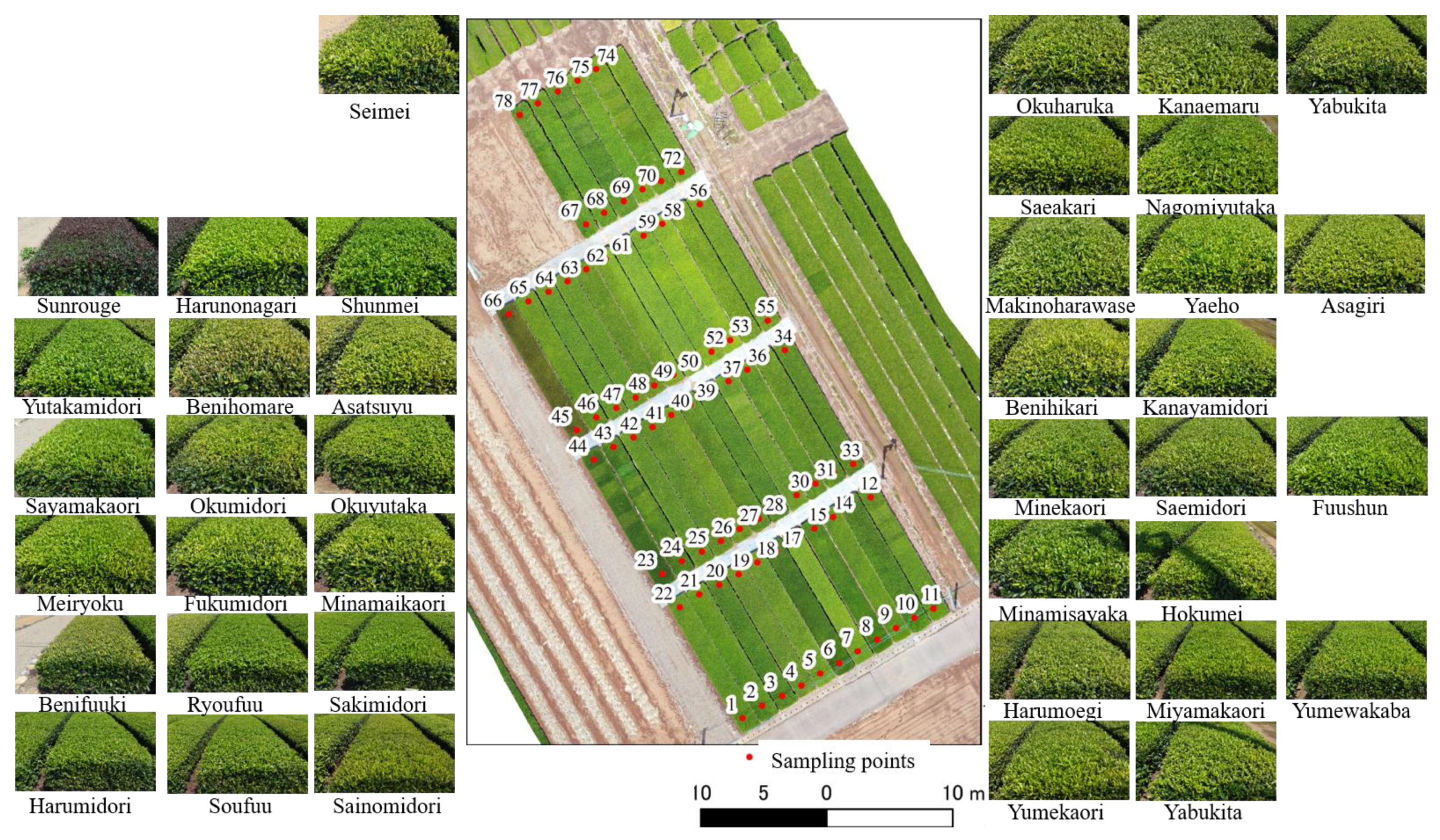
2.1. Measurements

The reflectance of tea plants was measured at the Institute of Fruit Tree and Tea Science, National Agriculture and Food Research Organization in Shimada, Japan. During the measurement period, the daily temperature ranged from 12.5 to 19.2 °C and daily precipitation was 0.0–17.5 mm. The tea field comprised 39 ridges with different cultivars on each ridge, except for the Yabukita cultivar, which was cultivated on two ridges (Figure 1). Most cultivars belonged to Camellia sinensis, except for Sunrouge (Camellia taliensis × C. sinensis). Yabukita is a well-known and widely cultivated tea cultivar in Japan and is used particularly for producing sencha. Many cultivars, including Fukumidori, Harumi-dori, Hokumei, Kanayamidori, Meiryoku, Minekaori, Okumidori, Ryoufuu, Saemidori, Sayamakaori, Soufuu, and Yumewakaba, are produced through crosses with Yabukita. From these, second filial generation cultivars such as Fuushun, Saeakari, Sainomidori, Seimei, Harumoegi, Kanaemaru, and Yumekaori are produced. While most of these cultivars are sencha-oriented, Sunrouge yields a pink tea and Benifuuki, Benihikari, and Benihomare are often used for black teas. We collected leaf samples from 38 tea cultivars at 78 different collection points on 10 May, 20 June, and 28 June. On each sampling date, 234 leaves were collected from the third leaf of the tea trees (three samples from each sampling point) to quantify carotenoid content and measure reflectance.

A spectrometer with a complementary metal-oxide semiconductor (CMOS) sensor (C12880MA, Hamamatsu Photonics) was used to measure reflectance. A shape-memory alloy (SMA)–SMA fiber patch cable (M25L05, Thorlabs) and a plant probe, which included a halogen light source, were connected to the spectrometer for direct measurements of individual leaves. This plant probe was created using the ASD Plant Probe as a reference [42].

The grating equations provided by Hamamatsu Photonics were applied and then the spectral resolution was resampled in 5 nm bands across the wavelength domain 400–850 nm. The reflectance of the target leaf was calculated using the following equation:

$${\rho }_{\lambda }=\frac{S_{\lambda }-D_{\lambda }}{W_{\lambda }-D_{\lambda }}$$

(1)

where S, W, and D are the target, diffuse reflectance standard, and dark current, respectively, at wavelength λ (in nm). All calculations were conducted using R version 4.2.2 [43].

Carotenoid content was quantified using a dual-beam scanning ultraviolet–visible spectrophotometer (UV-1280, Shimadzu, Japan). The equations used to quantify the carotenoids (μg mL⁻¹) in the N, N–dimethyl-formamide extracts were [11]:

$$\mathrm{Car}=\left(1000.00A_{480.0}-1.12C_a-34.07C_b\right)/245.00$$

(2)

$$C_a=12A_{663.8}-3.11A_{646.8}$$

(3)

$$C_b=20.78A_{646.8}-4.88A_{663.8}$$

(4)

where $\mathrm{Car}$, $C_a$, and $C_b$ represent the pigment contents of carotenoids, chlorophyll a, and b and A is the absorbance at the wavelength (nm) indicated by the subscript.

2.2. Adding Noise

Gaussian noise, also known as random noise or white noise, is characterized by a random distribution of values around the true signal that follows a Gaussian or normal distribution. Gaussian noise can arise from multiple sources, including noise introduced by electronic components, such as sensors, amplifiers, and digitizers, during the signal acquisition process. Electronic noise can also be introduced by external factors like electromagnetic interference from power lines, radio frequencies, or other nearby electronic devices, resulting in imperfections or variability in sensor responses over time.

Spike noise, also known as impulse noise or salt-and-pepper noise, manifests as sudden, isolated, and extreme outliers in the signal. These can be caused by momentary electrical disturbances or power surges and appear as spikes or abrupt jumps in the measurement system and data. Similar spikes can be produced during data transmission, resulting from errors due to faulty cables, connectors, or data corruption. Furthermore, certain sensor malfunctions or defects can produce sporadic spikes in the measurement data.

In this study, 125 sets of reflectance data with different noise patterns were generated by adding different amounts of Gaussian (zero mean and 0.01–0.05 variance) and spike noise (density of 0.01–0.05 and amplitude of 0.01–0.05) to the measured reflectance data.

2.3. Regression Models Based on Machine Learning Algorithms

After generating the noisy reflectance datasets, we divided each dataset into three groups using a stratified sampling approach: a training dataset (50%), a validation dataset (25%), and a test dataset (25%) [44]. The training datasets were used to generate regression models and the validation datasets were used to optimize the hyperparameters of the machine learning algorithms. Finally, the test datasets were used to evaluate model accuracy. This entire procedure was repeated 100 times to ensure the results were robust before the regression models were generated.

We used both Cubist and 1D-CNN to generate the regression models. Cubist employs a rule-based model tree approach, where leaves are represented by multivariate linear regression models. To refine the model predictions, we optimized the numbers of committee models (committee) and neighbors (neighbor) using the “Cubist” package [45]. Adjusting the committee models can yield a boosting effect, which was achieved here by implementing an ensemble approach combination where a nearest-neighbor algorithm was applied to the leaf nodes. A CNN is commonly used to automatically detect features of interest from a given dataset, and 1D-CNN can extract accurate features from 1D data [40]. We used the max-pooling technique and ReLU activation in the 1D-CNN. It has previously been demonstrated that 1D-CNN can effectively estimate the concentrations of major and minor pigments based on reflectance and absorption coefficient spectral inputs [40]. The architectural configuration we used consisted of 10 hidden layers, including four convolutional layers, four max-pooling layers, and two fully connected layers. We used dropout rates of 0.4 and 0.2, as suggested by the literature [46]. The regression models based on 1D-CNN were developed using Google Colaboratory [47].

2.4. Performance Assessment

To evaluate the performance of the regression models, we used three metrics: the ratio of performance to deviation (RPD) calculated using Equation (5) [48,49], where each method was classified into one of three categories (“A” (RPD > 2.0), “B” (1.4 ≥ RPD ≥ 2.0), or “C” (RPD < 1.4)) [50]; the root mean square error (RMSE, Equation (6) [51]); and the coefficient of determination (R², Equation (7) [52]). The formulae for these metrics are as follows:

$$\mathrm{RPD}=\mathrm{SD}/\mathrm{RMSE},$$

(5)

$$\mathrm{RMSE}=\sqrt{\frac{1}{n}{{\displaystyle \sum }}_{i=0}^n{\left(\widehat{y_i}-y_i\right)}^2},$$

(6)

$$R^2=1-\left(\frac{{{\displaystyle \sum }}_{i=1}^n{\left(y_i-\widehat{y_i}\right)}^2}{{{\displaystyle \sum }}_{i=1}^n{\left(y_i-\overline{y}\right)}^2}\right),$$

(7)

where SD is the standard deviation of the carotenoid content in the test data, n is the number of samples, $y_i$ is the measured carotenoid content, and $\widehat{y_i}$ is the estimated carotenoid content.

The variance principle can be used to evaluate the sensitivity of spectral wavelengths [46,53]. To calculate the sensitivity (S_i) for wavelength i (in nm), we used the following formula:

$$S_i=\frac{\mathrm{Var}(f\left(X_{400},\dots ,X_i,\dots ,X_{850}\right)-f\left(\overline{X}\right)}{\mathrm{Var}\left(Y\right)},$$

(8)

where Var is the variation, f() is the prediction of spectra resulting from the variation in wavelength i when other wavelengths are held constant at their mean values, f($\overline{X}$) is the estimated value based on the mean reflectance, and Y represents the measured carotenoid content. Once we had calculated S_i, we converted the scores to percentages.

3. Results

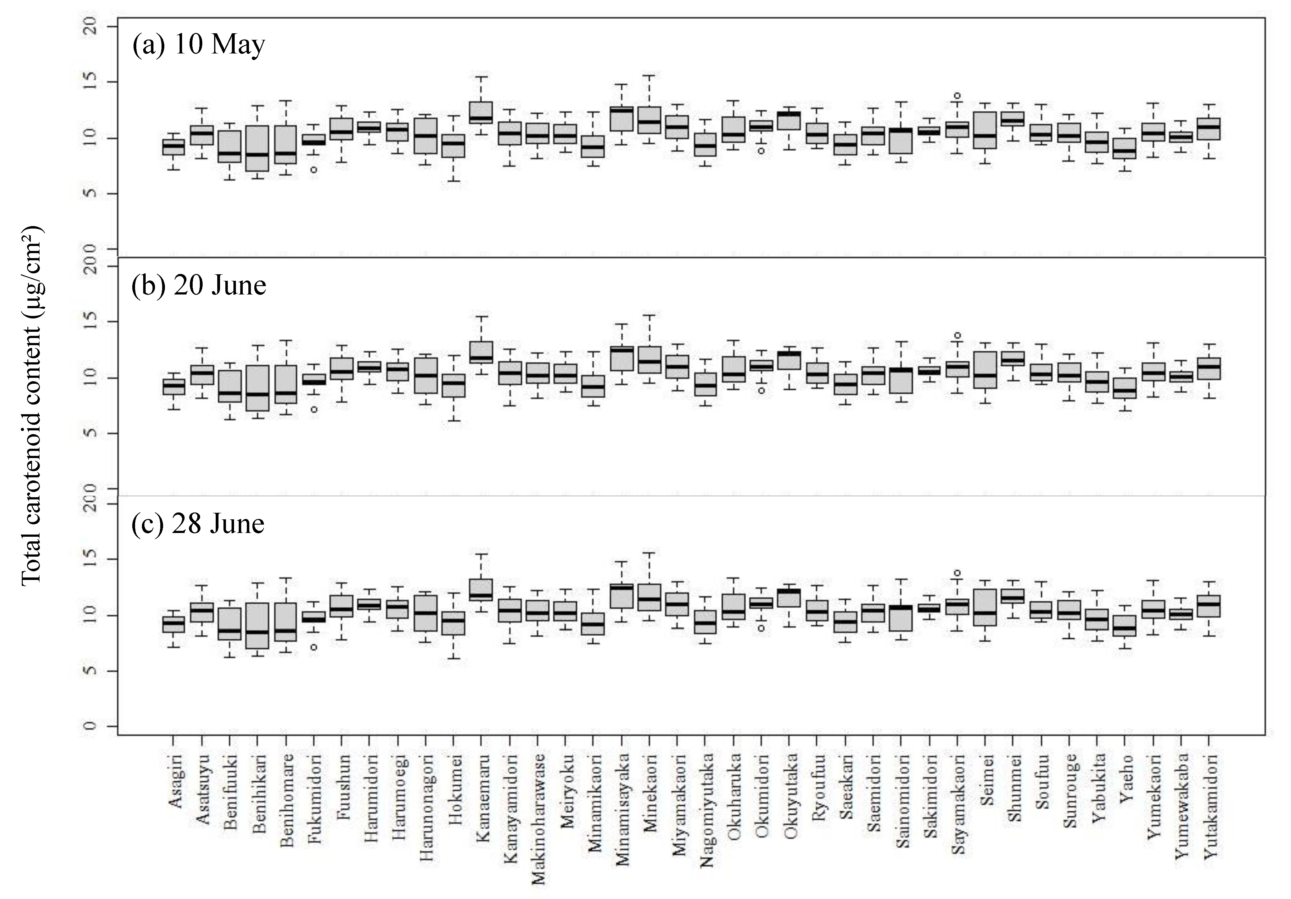
3.1. Carotenoid Content for Each Cultivar

The carotenoid content per cm² of leaf area was 6.18–15.63 µg and the averages for the three observation dates were 11.23, 10.28, and 9.45 µg, respectively. These differed significantly from each other, based on the Tukey–Kramer test (p < 0.001; Figure 2). Many of the lowest values were observed in black-tea-oriented cultivars (e.g., the mean carotenoid content of Benifuuki, Benihikari, and Benihomare was 8.89, 9.10, and 9.39 µg cm⁻², respectively), but the lowest value was observed in Hokumei (on 28 June). The cultivars with high values included matcha- and sencha-oriented cultivars (e.g., the mean carotenoid content of Kanaemaru, Minamisayaka, and Minekaori was 12.38, 11.99, and 11.70 µg cm⁻², respectively), and the highest value was observed in Minekaori (on 10 May).

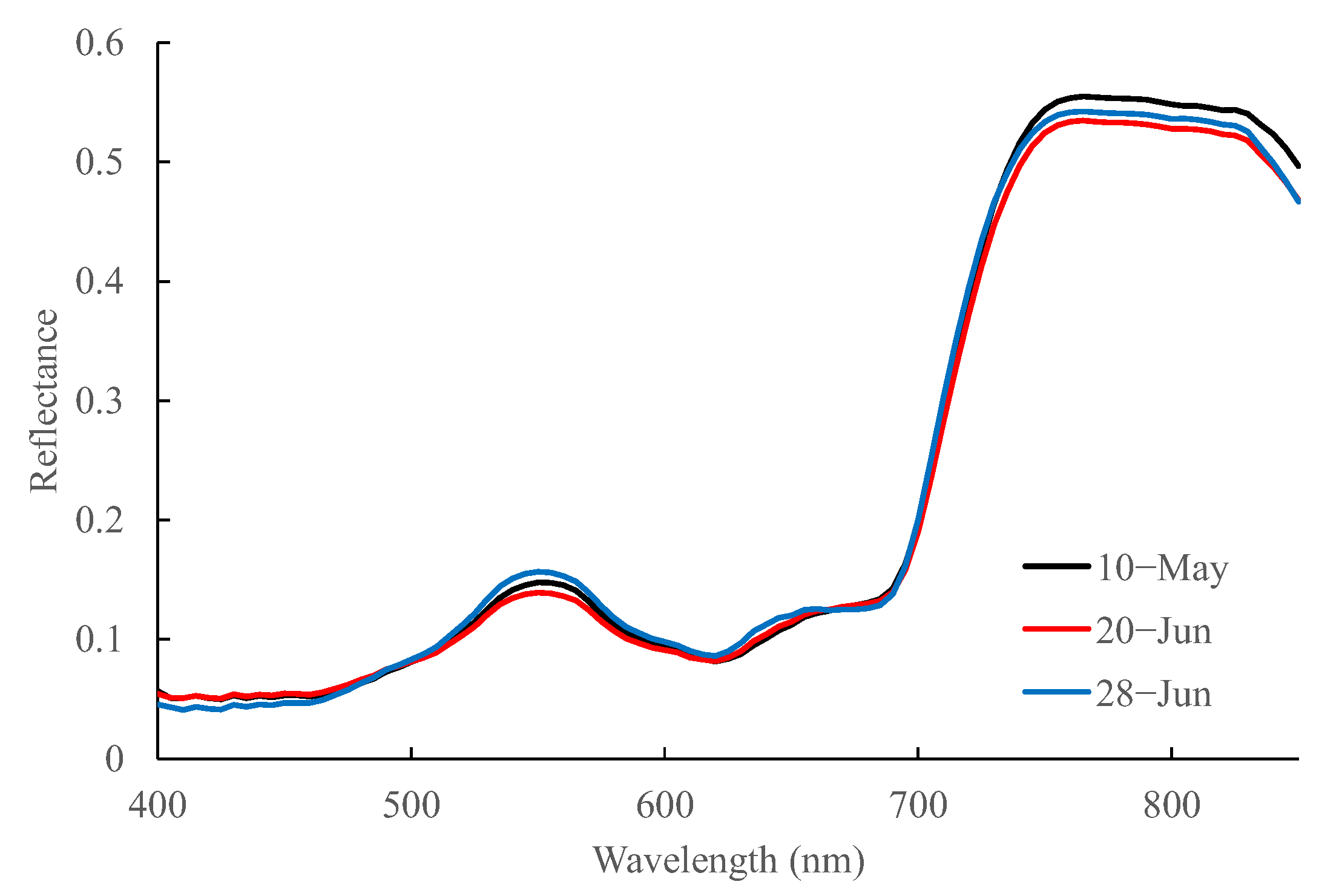
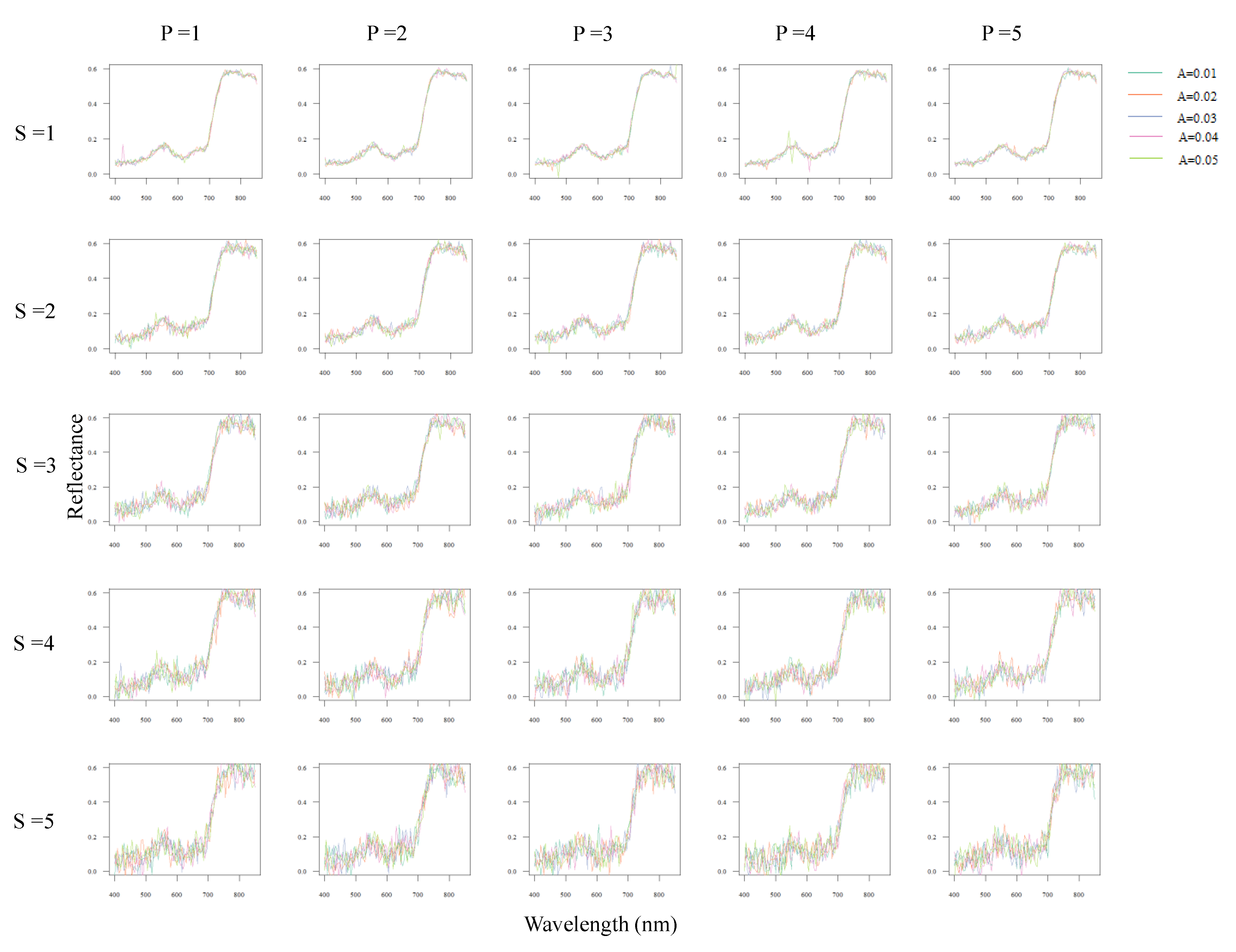
3.2. Spectral Reflectance

The mean reflectance of each date is shown in Figure 3. Chlorophyll absorption in the blue (400–500 nm) and red (600–700 nm) regions and the green peak, which is referred to as a distinct peak in the reflectance spectrum around 550–570 nm, was confirmed. In the transition region between the red and near-infrared, the red edge, which is a distinct feature in the reflectance spectrum of vegetation, was observed. Generally, the reflectance acquired on 20 June was the lowest and the reflectance acquired on 28 June was the highest over the green peak.

After obtaining the original reflectance data, 125 sets of reflectance data with different noise patterns were generated by adding different amounts of Gaussian (zero mean and 0.01–0.05 variance) and spike noise (density of 0.01–0.05 and amplitude of 0.01–0.05). Figure 4 shows a sample of the reflectance sets with different amounts of Gaussian and spike noise.

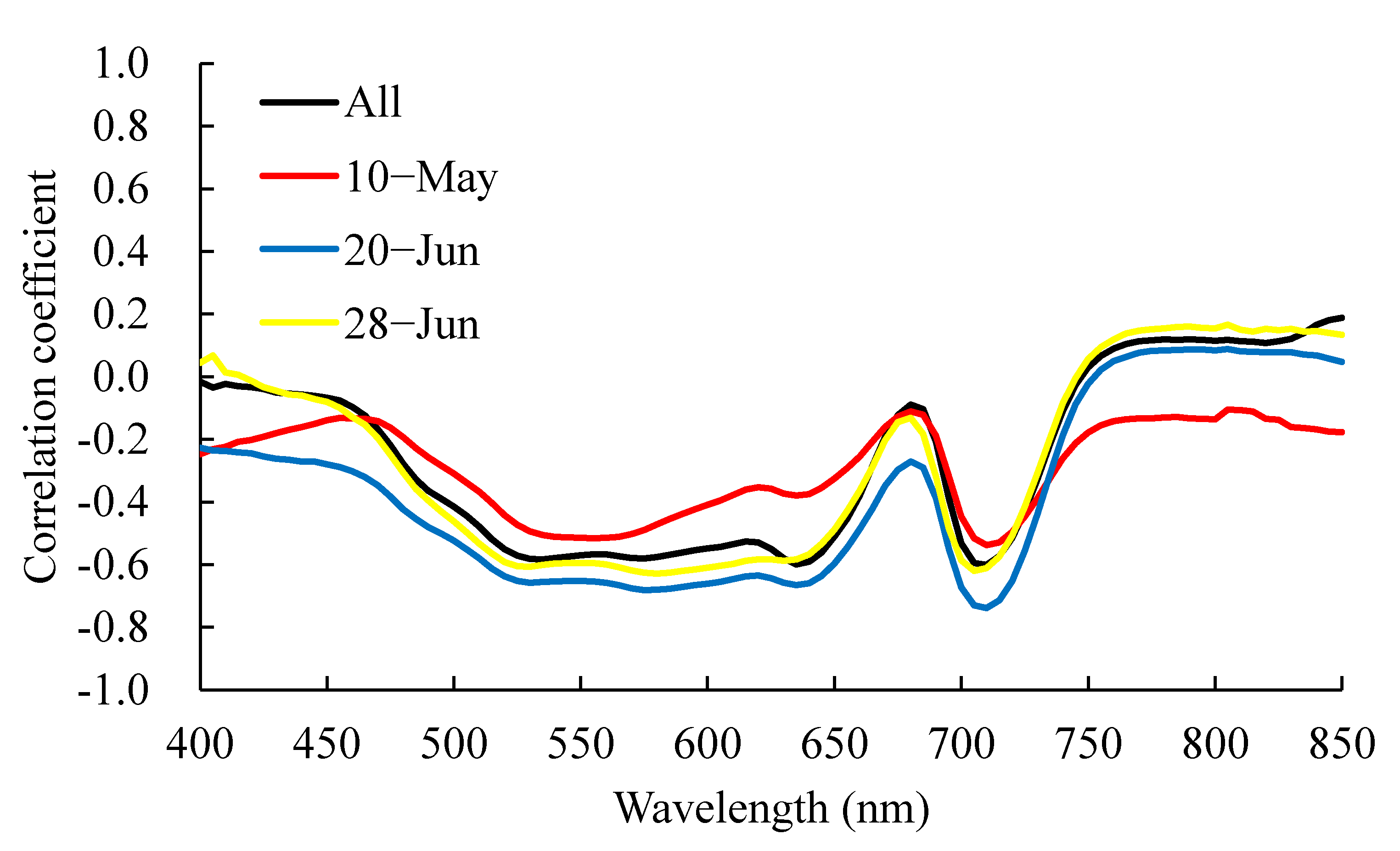
3.3. Correlation between Carotenoid Content and Reflectance

Two valleys are apparent in the graph of correlation coefficients for all dates (500–650 and 700–710 nm; r: −0.60 to −0.51; p < 0.001; Figure 5). The correlations were weaker on the first sampling day than on the other dates.

Lasso regression analysis revealed that Gaussian noise influenced the correlation coefficients at 550 nm and that the correlations became weaker as the Gaussian noise increased. The lowest values on the different sampling dates ranged from −0.49 to −0.56, −0.41 to −0.50, −0.34 to −0.44, −0.24 to −0.39, and −0.18 to −0.32, respectively, for Gaussian noise variance values of 0.01, 0.02, 0.03, 0.04, and 0.05.

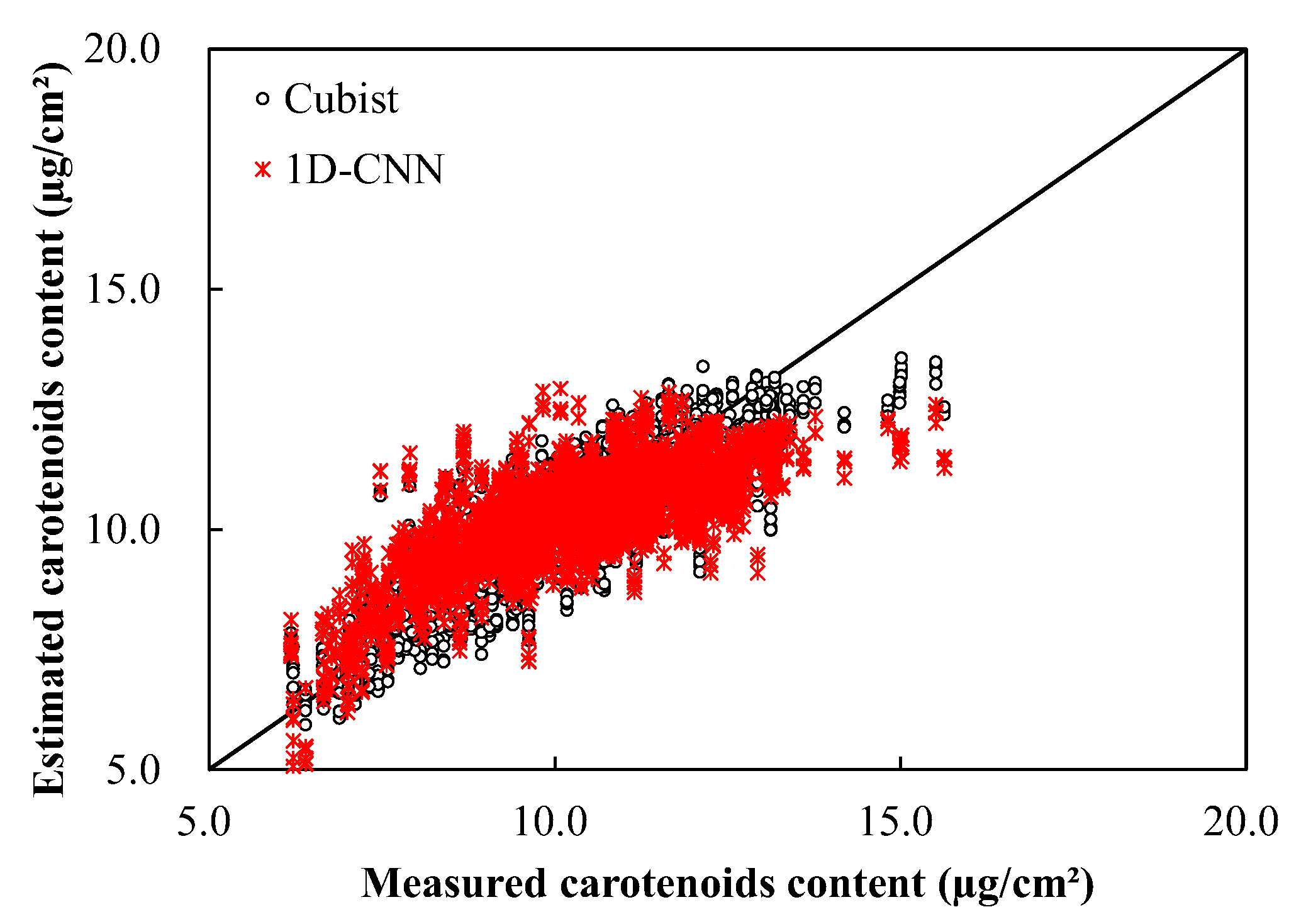
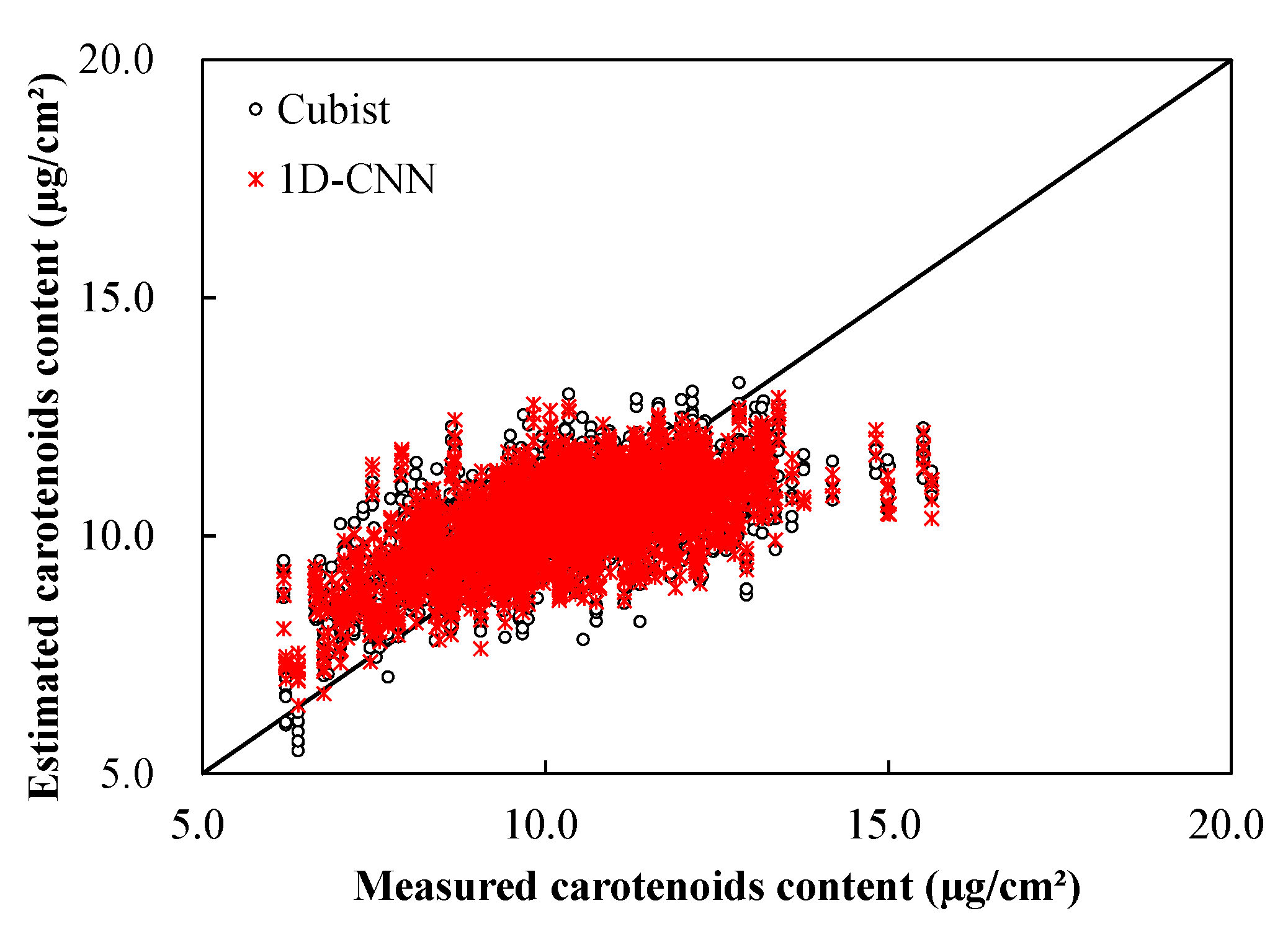
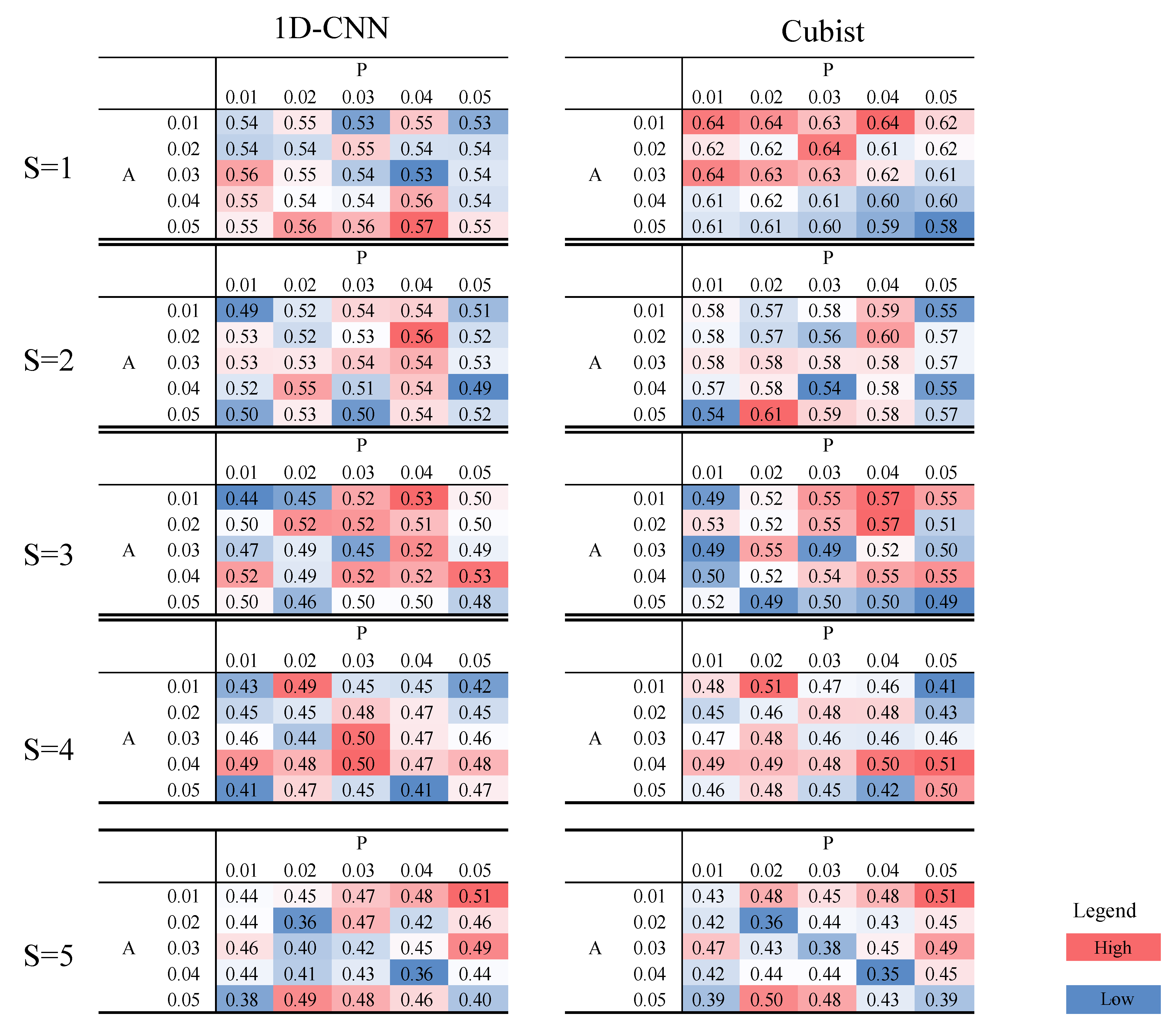
3.4. Accuracy Assessment

The models based on both algorithms were able to reliably estimate carotenoid content, although the Cubist-based regression model performed better, achieving an RPD value greater than 2.0 (

Table 1. Estimation accuracies based on actual reflectance measurements from a compact spectrometer.

RPD		RMSE (µg/cm2)		R2
1D-CNN	Cubist	1D-CNN	Cubist	1D-CNN	Cubist
1.50	2.05	1.03	0.76	0.56	0.76

).

Although both machine learning algorithms had low estimation accuracies for cultivars with a high carotenoid content (e.g., Kanaemaru and Minekaori), Cubist had a higher accuracy for cultivars with a low carotenoid content (e.g., Benifuuki and Benihomare) (Figure 6). However, the estimation abilities of Cubist and 1D-CNN were more similar for cultivars with a high carotenoid content when high levels of noise were added to the reflectance data (Figure 7).

The calculated RPD, RMSE, and R² values for the regression models applied to datasets with different each noise levels are shown in Figure 8, Figure 9 and Figure 10, respectively. The 1D-CNN-based model performed better than the Cubist-based model when the Gaussian noise variance values were less than 0.01, and it even achieved an RPD of 1.50 for the dataset with Gaussian noise variance of 0.02 and a spike noise amplitude of 0.02 and density of 0.04 (Figure 8). This contrasted with the accuracy of the Cubist-based regression model, which decreased obviously with increased noise levels. However, both algorithms achieved acceptable estimation results, meeting the threshold of RPD > 1.4 when the Gaussian noise variance was less than 0.02. Cubist remained effective for datasets with Gaussian noise variance values as high as 0.03. Generally, the Cubist algorithm produced higher accuracy; however, when the Gaussian noise variance exceeded 0.04 and the amplitude and density of the spike noise were 0.03, the 1D-CNN-based regression models were more accurate.

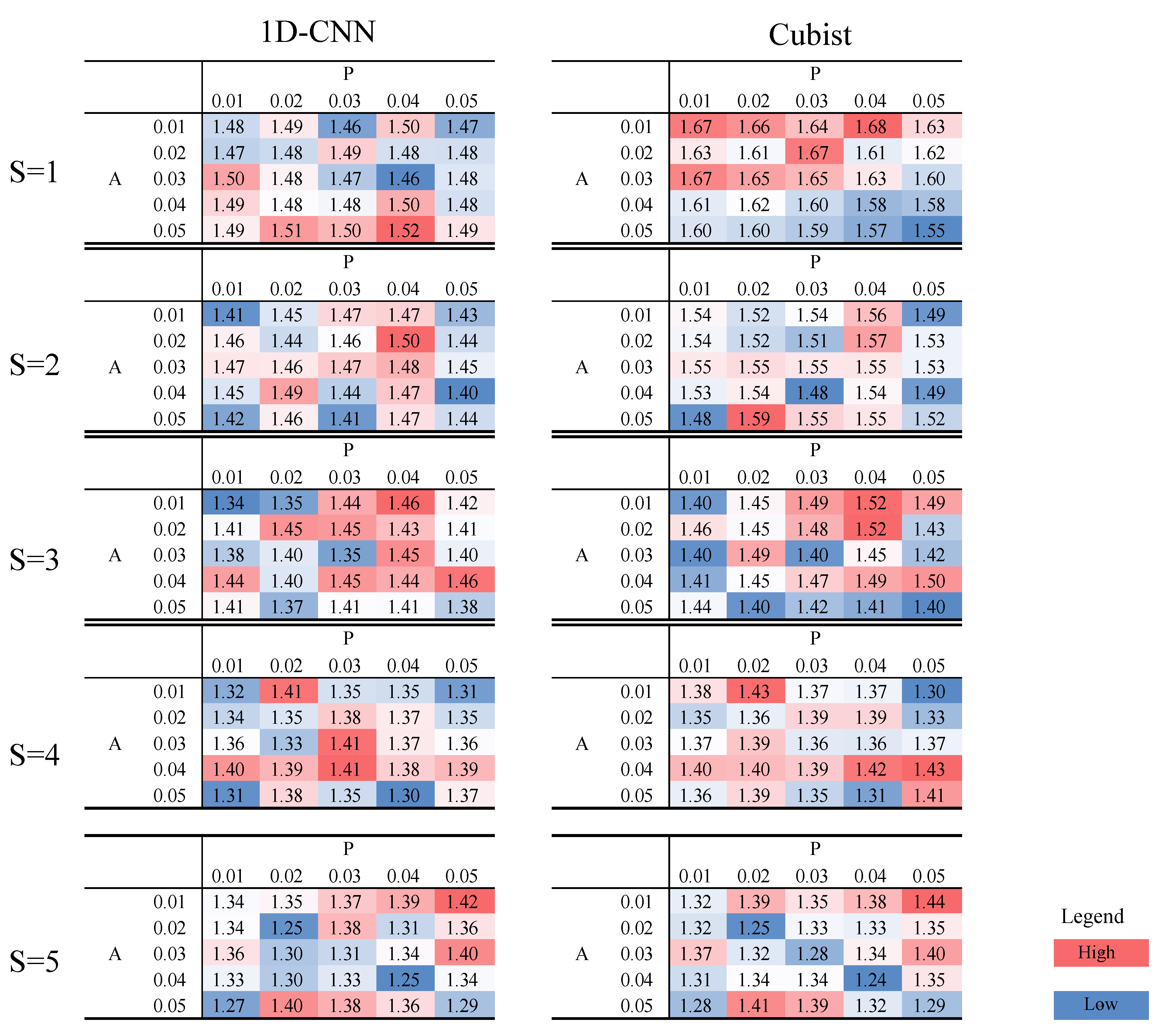
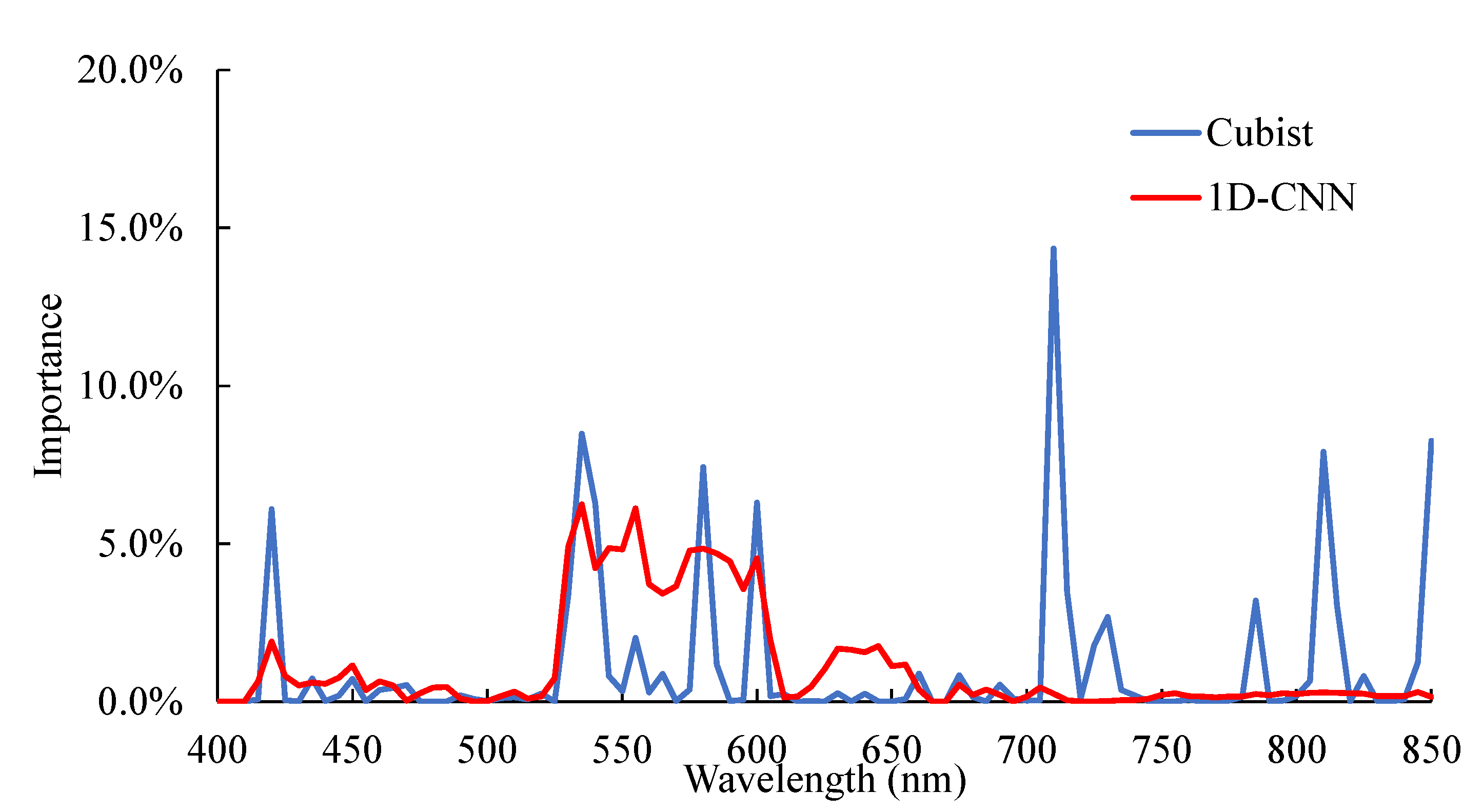
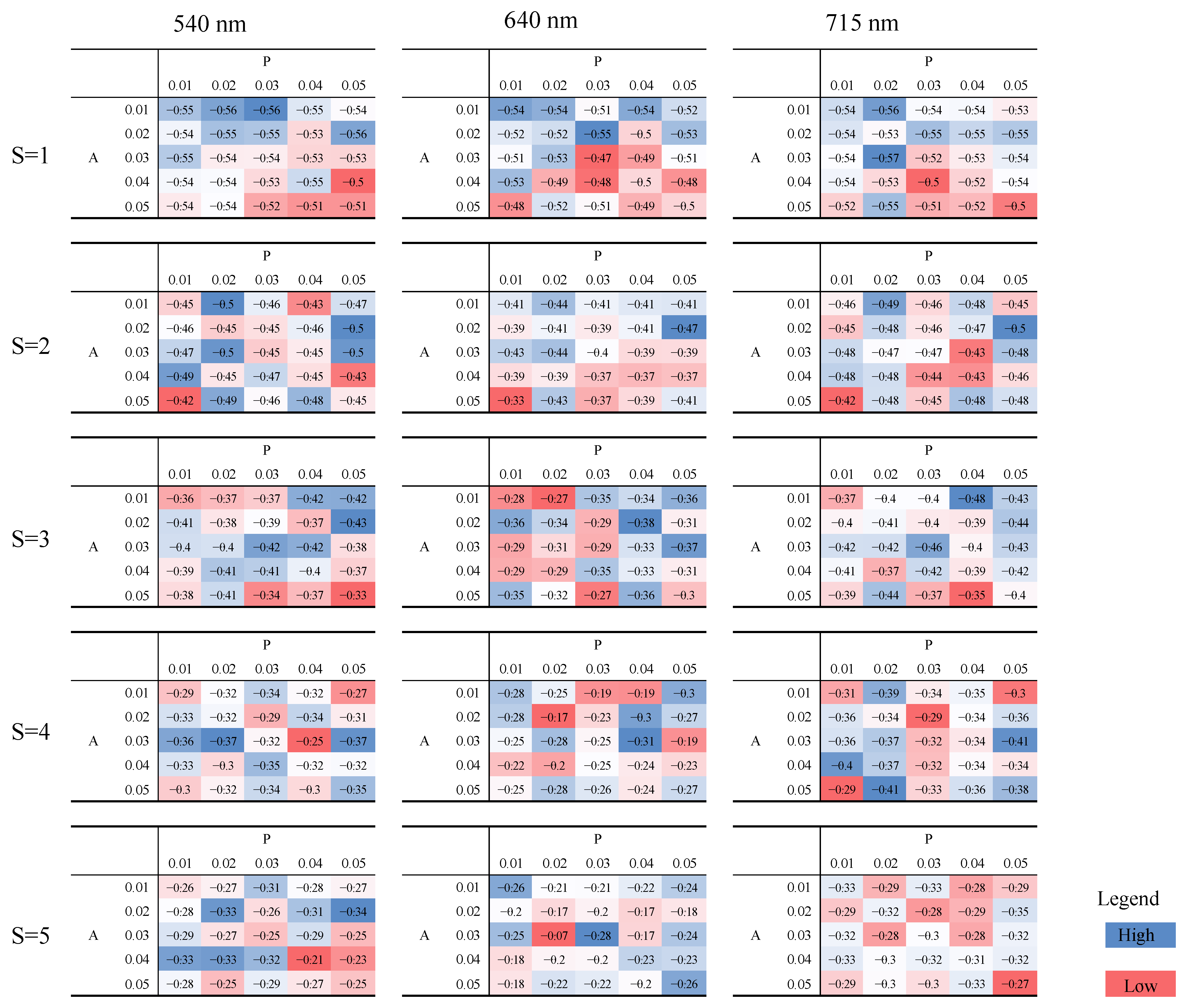
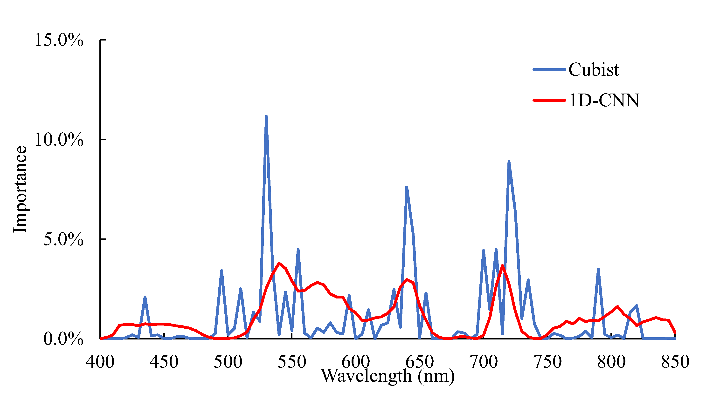
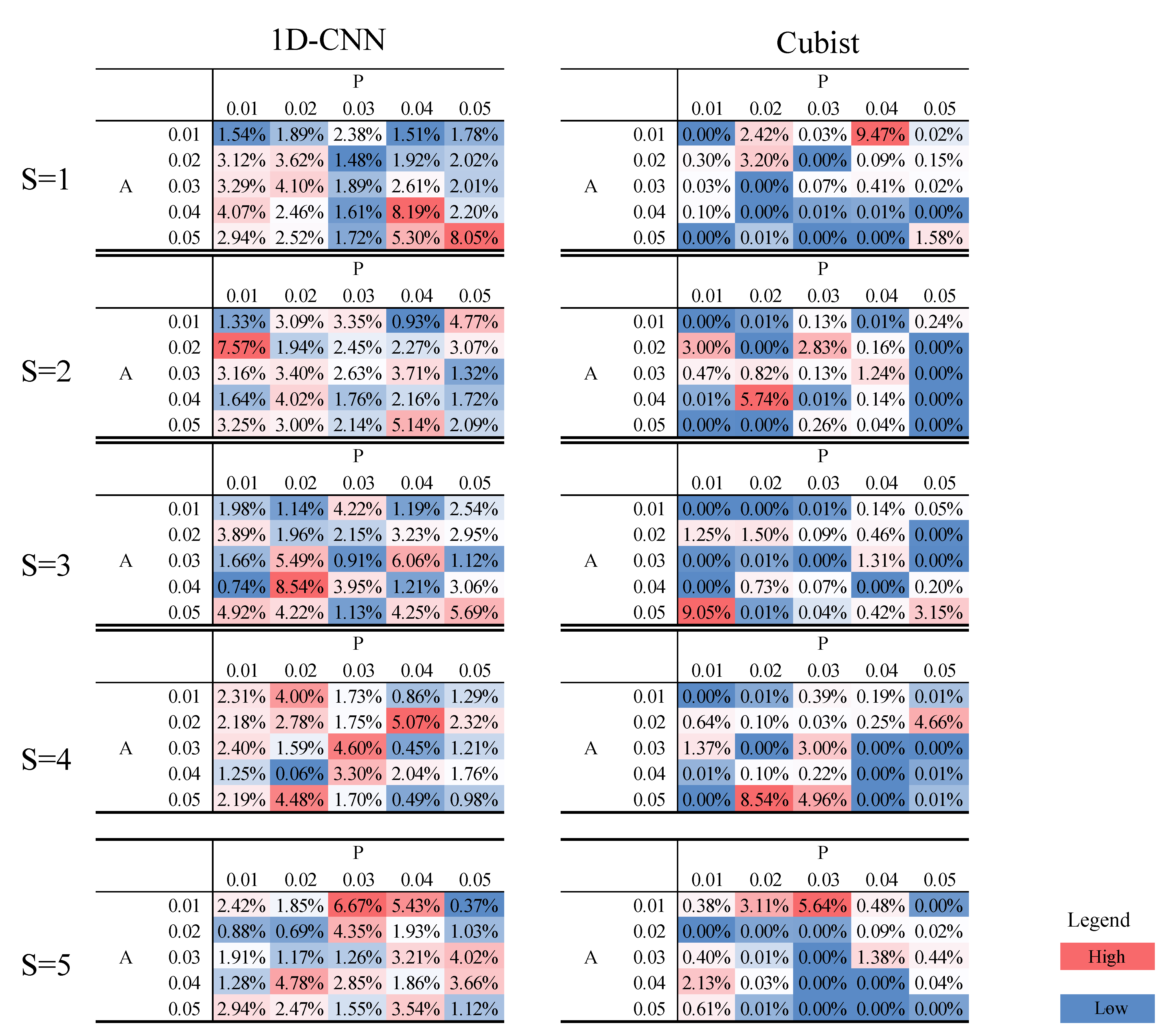
3.5. Sensitivity Analysis

The sensitivity analysis of the regression models using the original reflectance dataset revealed three peaks around 550, 650, and 715 nm for both machine learning algorithms (Figure 11). However, for Cubist-based models, the distribution of importance showed specific wavelength ranges with extremely high values, while the distribution for the 1D-CNN-based model was more even.

When the sensitivity analysis was applied to noisy reflectance data, the peak around 650 nm was not present for either algorithm and the peak around 715 nm was lost for the 1D-CNN-based model, but it persisted for the Cubist-based model (Figure 12).

4. Discussion

4.1. Accuracy Assessment

Various algorithms have been used to estimate carotenoid content based on reflectance data, and each algorithm has performed differently (

Table 2. Literature review summary of algorithm accuracies based on measured reflectance datasets.

Sample	Accuracy	Algorithm	Reference
Forest leaves included in ANGERS (measured with ASD FieldSpec)	RMSE = 2.6019 μg/m2 R2 = 0.74	Convolution neural network	[54]
Australian eucalypt species (measured with ASD FieldSpec 3)	RMSE = 3.83 μg/m2 NRMSE = 30.82%	Inversion of the Fluspect-Cx Model	[55]
Japanese horseradish (measured with ASD FieldSpec 4)	RPD = 1.63–3.32 RMSE = 0.31–1.89 μg/m2	SNV and Cubist	[56]
Maple and chestnut (measured with Hitachi 150-20 spectrophotometer), beech (measured with Shimatzu 2101 PC spectrophotometer)	R2 = 0.71 RMSE = 1.86 nmol/cm2	Spectral indices	[32]

). Further, although the study area and species of vegetation in the present study differed from those in these previous studies, all the reflectance values were measured using commercial spectrometers. Applying the Cubist algorithm in the proposed system produced carotenoid estimation accuracies comparable to those of the commercial spectrometer.

Noise injection is often used to augment data when applying machine learning and deep learning techniques [57,58]. Noise acts as a form of regularization in regression models, aiding in the prevention of overfitting. Overfitting occurs when a model becomes overly specialized to the training data and can no longer effectively generalize to unseen data [59]. By introducing noise during training, noisy or irrelevant patterns in the data can be obscured, forcing the model to generalize and capture the more robust features. In addition, machine learning models are vulnerable to adversarial attacks, where intentionally designed perturbations in the input data can mislead the model and lead to incorrect predictions [60,61]. Normally, the carotenoid content is low relative to chlorophyll content, so the RPD values of carotenoid estimation models have generally been worse than those of chlorophyll estimation models. By training the model with noisy samples, it becomes more resilient to adversarial perturbations, making model outputs more reliable. Indeed, 1D-CNN-based models have performed better than least-squares support vector machine, artificial neural network, long short-term memory, and gated recurrent unit models [62,63]. In this study, the Cubist-based model was also robust when estimating carotenoid content from reflectance data, even though Cubist-based models are generally most accurate when applied to denoised reflectance data [56,64].

4.2. Sensitivity Analysis

The red edge phenomenon pertains to the rapid increase in reflectance that occurs in the transitional region between the red and near-infrared wavelengths in the reflectance spectrum of green vegetation. Carotenoids strongly absorb light in the blue and green spectral region [65,66], but their absorption diminishes in the red and near-infrared regions, while chlorophyll strongly absorbs light in the blue and red regions and reflects more strongly in the green and near-infrared regions [65]. As a result, the presence of carotenoids affects reflectance at the green peak (around 550 nm), the red edge inflection point (REIP, around 650 nm), and the peak around 715 nm.

In this study, although the spectrometer measured reflectance data across the entire wavelength domain from 400 to 850 nm, the relative sensitivity of its sensor was < 0.5 at 700 nm [67]. Despite this, the heightened reflectance around 715 nm was still clearly observable. Therefore, the plant probe effectively placed the sensor at an appropriate location to receive the most accurate and representative readings, enabling measurements at wavelengths over 700 nm to be used for estimating carotenoids. However, the heightened reflectance at 650 nm disappeared when noise was injected into the dataset. Figure 13 shows the coefficients of the correlations between carotenoid content and reflectance at 540, 640, and 715 nm when injecting different levels of noise. Adding Gaussian noise with a variance of 0.04–0.05 produced uncertainty in the reflectance data over the REIP and reduced the correlation coefficients to below −0.2. As a result, the importance of 640 nm for estimating carotenoid content disappeared when using noisy reflectance data.

The reflectance values at 650 nm ranged from 0.07 (Miyamakaori on 20 June) to 0.19 (Benihikari on 20 June), which was a relatively small range (the smallest difference was 0.08 at 760 nm). Therefore, this domain was quite susceptible to noise injections. Figure 14 shows the importance of reflectance at 650 nm for models based on both algorithms at different noise intensities. Adding noise reduced the importance of the 650 nm wavelength and the decrease in importance was quite significant, although the importance sometimes exceeded 9.0% under low density or low amplitude conditions.

Carotenoids absorb light at wavelengths from 400 to 700 nm [35]. Specifically, the green peak has been used for carotenoid contents in previous studies. However, some reflectance values at 700–780 nm possessed certain importance for estimating carotenoid content estimation when Cubist-based regression models were applied. This peak is influenced by the presence of chlorophyll and carotenoids in the leaves. On the contrary, the red edge is closely related to the absorption characteristics of chlorophyll. Therefore, the combined use of the green peak and the red edge is effective in mitigating the influence of chlorophyll for retrieving carotenoid content from reflectance.

Remote sensing utilizing hyperspectral reflectance offers a robust perspective for estimating carotenoid content in vegetation since carotenoids leave a distinctive imprint on spectral signatures. Hyperspectral sensors capture a vast range of narrow, contiguous bands across the electromagnetic spectrum, enabling precise characterization of these signatures and then spectral indices tailored to carotenoid absorption features. However, airborne or satellite-based hyperspectral acquisitions facilitate large-scale assessments, their measurements include some noises [68,69], and employing spectral indices is challenging to accurately assess carotenoid content. By bridging small-scale measurements with comprehensive observations, hyperspectral remote sensing empowers resource-efficient land management and contributes to sustainable ecosystem stewardship.

5. Conclusions

In this study, we proposed a system to estimate the carotenoid content of tea leaves based on micro-spectrometer (C12880MA, Hamamatsu Photonics) measurements. The proposed system achieved highly accurate carotenoid content estimations using the carotenoid measurements and Cubist-based regression models, confirming the effectiveness of the system. Next, we artificially introduced Gaussian and spike noise, which can result from factors such as electrical components, faulty data transmission, or environmental conditions, to the measured reflectance data to evaluate the models’ robustness against noise. When comparing the Cubist and 1D-CNN-based estimation models, the Cubist model generally produced better estimation results. However, the accuracy of the Cubist-based model degraded more rapidly because of increasing noise intensity than that of the 1D-CNN-based model.

References

1. Palace, V.P.; Khaper, N.; Qin, Q.; Singal, P.K. Antioxidant potentials of vitamin A and carotenoids and their relevance to heart disease. Free. Radic. Biol. Med. 1999, 26, 746–761. [Google Scholar] [CrossRef] [PubMed]
2. Maoka, T. Carotenoids as natural functional pigments. J. Nat. Med. 2020, 74, 1–16. [Google Scholar] [CrossRef] [PubMed]
3. Crupi, P.; Faienza, M.F.; Naeem, M.Y.; Corbo, F.; Clodoveo, M.L.; Muraglia, M. Overview of the Potential Beneficial Effects of Carotenoids on Consumer Health and Well-Being. Antioxidants 2023, 12, 1069. [Google Scholar] [CrossRef] [PubMed]
4. Elvira-Torales, L.I.; García-Alonso, J.; Periago-Castón, M.J. Nutritional Importance of Carotenoids and Their Effect on Liver Health: A Review. Antioxidants 2019, 8, 229. [Google Scholar] [CrossRef] [PubMed]
5. Demmig-Adams, B.; Gilmore, A.M.; Adams, W.W. Carotenoids 3: In Vivo Function of Carotenoids in Higher Plants. FASEB J. 1996, 10, 403–412. [Google Scholar] [CrossRef] [PubMed]
6. Edge, R.; McGarvey, D.; Truscott, T. The carotenoids as anti-oxidants—A review. J. Photochem. Photobiol. B Biol. 1997, 41, 189–200. [Google Scholar] [CrossRef]
7. Yang, Y.-Z.; Li, T.; Teng, R.-M.; Han, M.-H.; Zhuang, J. Low temperature effects on carotenoids biosynthesis in the leaves of green and albino tea plant (Camellia sinensis (L.) O. Kuntze). Sci. Hortic. 2021, 285, 110164. [Google Scholar] [CrossRef]
8. Chen, Y.; Niu, S.; Deng, X.; Song, Q.; He, L.; Bai, D.; He, Y. Genome-wide association study of leaf-related traits in tea plant in Guizhou based on genotyping-by-sequencing. BMC Plant Biol. 2023, 23, 196. [Google Scholar] [CrossRef]
9. Baker, R.; Günther, C. The Role of Carotenoids in Consumer Choice and the Likely Bene Wts from Their Inclusion into Products for Human Consumption. Trends Food Sci. Technol. 2004, 15, 484–488. [Google Scholar] [CrossRef]
10. Smith, R.M. High-Performance Liquid Chromatography—Advances and Perspectives. J. Pharm. Biomed. Anal. 1984, 2, 567. [Google Scholar] [CrossRef]
11. Wellburn, A.R. The Spectral Determination of Chlorophylls a and b, as well as Total Carotenoids, Using Various Solvents with Spectrophotometers of Different Resolution. J. Plant Physiol. 1994, 144, 307–313. [Google Scholar] [CrossRef]
12. Seoudi, R.; El-Bahy, G.; El Sayed, Z. Ultraviolet and visible spectroscopic studies of phthalocyanine and its complexes thin films. Opt. Mater. 2006, 29, 304–312. [Google Scholar] [CrossRef]
13. Prasad, K.A.; Gnanappazham, L.; Selvam, V.; Ramasubramanian, R.; Kar, C.S. Developing a spectral library of mangrove species of Indian east coast using field spectroscopy. Geocarto Int. 2015, 30, 580–599. [Google Scholar] [CrossRef]
14. Cristóbal, J.; Graham, P.; Prakash, A.; Buchhorn, M.; Gens, R.; Guldager, N.; Bertram, M. Airborne Hyperspectral Data Acquisition and Processing in the Arctic: A Pilot Study Using the Hyspex Imaging Spectrometer for Wetland Mapping. Remote Sens. 2021, 13, 1178. [Google Scholar] [CrossRef]
15. Qamar, F.; Sharma, M.S.; Dobler, G. The Impacts of Air Quality on Vegetation Health in Dense Urban Environments: A Ground-Based Hyperspectral Imaging Approach. Remote Sens. 2022, 14, 3854. [Google Scholar] [CrossRef]
16. Shaik, R.U.; Periasamy, S.; Zeng, W. Potential Assessment of PRISMA Hyperspectral Imagery for Remote Sensing Applications. Remote Sens. 2023, 15, 1378. [Google Scholar] [CrossRef]
17. Sonobe, R.; Miura, Y.; Sano, T.; Horie, H. Monitoring Photosynthetic Pigments of Shade-Grown Tea from Hyperspectral Reflectance. Can. J. Remote Sens. 2018, 44. [Google Scholar] [CrossRef]
18. Sonobe, R.; Sano, T.; Horie, H. Using spectral reflectance to estimate leaf chlorophyll content of tea with shading treatments. Biosyst. Eng. 2018, 175, 168–182. [Google Scholar] [CrossRef]
19. Sonobe, R.; Hirono, Y.; Oi, A. Non-Destructive Detection of Tea Leaf Chlorophyll Content Using Hyperspectral Reflectance and Machine Learning Algorithms. Plants 2020, 9, 368. [Google Scholar] [CrossRef]
20. Sonobe, R.; Hirono, Y.; Oi, A. Quantifying chlorophyll-a and b content in tea leaves using hyperspectral reflectance and deep learning. Remote Sens. Lett. 2020, 11, 933–942. [Google Scholar] [CrossRef]
21. Zarco-Tejada, P.J.; Berjón, A.; López-Lozano, R.; Miller, J.R.; Martín, P.; Cachorro, V.; González, M.R.; De Frutos, A. Assessing vineyard condition with hyperspectral indices: Leaf and canopy reflectance simulation in a row-structured discontinuous canopy. Remote Sens. Environ. 2005, 99, 271–287. [Google Scholar] [CrossRef]
22. Gautam, D.; Lucieer, A.; Watson, C.; McCoull, C. Lever-arm and boresight correction, and field of view determination of a spectroradiometer mounted on an unmanned aircraft system. ISPRS J. Photogramm. Remote Sens. 2019, 155, 25–36. [Google Scholar] [CrossRef]
23. Sonobe, R.; Hirono, Y. Applying Variable Selection Methods and Preprocessing Techniques to Hyperspectral Reflectance Data to Estimate Tea Cultivar Chlorophyll Content. Remote Sens. 2023, 15, 19. [Google Scholar] [CrossRef]
24. Sonobe, R.; Yamashita, H.; Nofrizal, A.Y.; Seki, H.; Morita, A.; Ikka, T. Use of spectral reflectance from a compact spectrometer to assess chlorophyll content in Zizania latifolia. Geocarto Int. 2022, 37, 5363–5375. [Google Scholar] [CrossRef]
25. Shao, Y.; He, Y.; Bao, Y.; Mao, J. Near-Infrared Spectroscopy for Classification of Oranges and Prediction of the Sugar Content. Int. J. Food Prop. 2009, 12, 644–658. [Google Scholar] [CrossRef]
26. Barnes, R.J.; Dhanoa, M.S.; Lister, S.J. Standard Normal Variate Transformation and De-Trending of Near-Infrared Diffuse Reflectance Spectra. Appl. Spectrosc. 1989, 43, 772–777. [Google Scholar] [CrossRef]
27. Jamshidi, B.; Minaei, S.; Mohajerani, E.; Ghassemian, H. Reflectance Vis/NIR spectroscopy for nondestructive taste characterization of Valencia oranges. Comput. Electron. Agric. 2012, 85, 64–69. [Google Scholar] [CrossRef]
28. Mishra, P.; Karami, A.; Nordon, A.; Rutledge, D.N.; Roger, J.-M. Automatic de-noising of close-range hyperspectral images with a wavelength-specific shearlet-based image noise reduction method. Sens. Actuators B Chem. 2019, 281, 1034–1044. [Google Scholar] [CrossRef]
29. Karami, A.; Heylen, R.; Scheunders, P. Band-Specific Shearlet-Based Hyperspectral Image Noise Reduction. IEEE Trans. Geosci. Remote Sens. 2015, 53, 5054–5066. [Google Scholar] [CrossRef]
30. Vorasayan, P.; Suwanwela, N.C.; Auethavekiat, S.; Chinrungrueng, C.; Sa-Ing, V. Multiscale adaptive regularisation Savitzky–Golay method for speckle noise reduction in ultrasound images. IET Image Process. 2018, 12, 105–112. [Google Scholar] [CrossRef]
31. Zimmermann, B.; Kohler, A. Optimizing Savitzky-Golay Parameters for Improving Spectral Resolution and Quantification in Infrared Spectroscopy. Appl. Spectrosc. 2013, 67, 892–902. [Google Scholar] [CrossRef] [PubMed]
32. Gitelson, A.A.; Zur, Y.; Chivkunova, O.B.; Merzlyak, M.N. Assessing Carotenoid Content in Plant Leaves with Reflectance Spectroscopy. Photochem. Photobiol. 2002, 75, 272–281. [Google Scholar] [CrossRef] [PubMed]
33. Gamon, J.A.; Peñuelas, J.; Field, C.B. A narrow-waveband spectral index that tracks diurnal changes in photosynthetic efficiency. Remote Sens. Environ. 1992, 41, 35–44. [Google Scholar] [CrossRef]
34. Penuelas, J.; Baret, F.; Filella, I. Semi-Empirical Indices to Assess Carotenoids/Chlorophyll a Ratio from Leaf Spectral Re-flectance. Photosynthetica 1995, 31, 221–230. [Google Scholar]
35. Féret, J.-B.; Gitelson, A.; Noble, S.; Jacquemoud, S. PROSPECT-D: Towards modeling leaf optical properties through a complete lifecycle. Remote Sens. Environ. 2017, 193, 204–215. [Google Scholar] [CrossRef]
36. Sonobe, R.; Miura, Y.; Sano, T.; Horie, H. Estimating leaf carotenoid contents of shade-grown tea using hyperspectral indices and PROSPECT–D inversion. Int. J. Remote Sens. 2018, 39, 1306–1320. [Google Scholar] [CrossRef]
37. Fernández-Delgado, M.; Sirsat, M.; Cernadas, E.; Alawadi, S.; Barro, S.; Febrero-Bande, M. An extensive experimental survey of regression methods. Neural Netw. 2019, 111, 11–34. [Google Scholar] [CrossRef]
38. Alkhayrat, M.; Aljnidi, M.; Aljoumaa, K. A comparative dimensionality reduction study in telecom customer segmentation using deep learning and PCA. J. Big Data 2020, 7, 9. [Google Scholar] [CrossRef]
39. Sakurada, M.; Yairi, T. Anomaly Detection Using Autoencoders with Nonlinear Dimensionality Reduction. In Proceedings of the ACM International Conference Proceeding Series, Montreal, QC, Canada, 8–13 December 2014; Volume 2. [Google Scholar]
40. Ng, W.; Minasny, B.; Montazerolghaem, M.; Padarian, J.; Ferguson, R.; Bailey, S.; McBratney, A.B. Convolutional neural network for simultaneous prediction of several soil properties using visible/near-infrared, mid-infrared, and their combined spectra. Geoderma 2019, 352, 251–267. [Google Scholar] [CrossRef]
41. Pullanagari, R.; Dehghan-Shoar, M.; Yule, I.J.; Bhatia, N. Field spectroscopy of canopy nitrogen concentration in temperate grasslands using a convolutional neural network. Remote Sens. Environ. 2021, 257, 112353. [Google Scholar] [CrossRef]
42. Malvern Panalytical. ASD Plant Probe. Available online: https://www.azom.com/equipment-details.aspx?EquipID=5412 (accessed on 19 July 2023).
43. R Core Team. R: A Language and Environment for Statistical Computing. Available online: https://www.R-project.org/ (accessed on 19 July 2023).
44. Ruppert, D. The Elements of Statistical Learning: Data Mining, Inference, and Prediction. J. Am. Stat. Assoc. 2004, 99, 567. [Google Scholar] [CrossRef]
45. Kuhn, M.; Weston, S.; Keefer, C.; Coulter, N.; Quinlan, R. Rulequest Research Pty Ltd. Package ‘Cubist’. Available online: https://cran.r-project.org/web/packages/Cubist/Cubist.pdf (accessed on 19 July 2023).
46. Kawamura, K.; Nishigaki, T.; Andriamananjara, A.; Rakotonindrina, H.; Tsujimoto, Y.; Moritsuka, N.; Rabenarivo, M.; Razafimbelo, T. Using a One-Dimensional Convolutional Neural Network on Visible and Near-Infrared Spectroscopy to Improve Soil Phosphorus Prediction in Madagascar. Remote Sens. 2021, 13, 1519. [Google Scholar] [CrossRef]
47. Bisong, E. Google Colaboratory. In Building Machine Learning and Deep Learning Models on Google Cloud Platform; Apress: Berkeley, CA, USA, 2019. [Google Scholar] [CrossRef]
48. Bellon-Maurel, V.; Fernandez-Ahumada, E.; Palagos, B.; Roger, J.-M.; McBratney, A. Critical review of chemometric indicators commonly used for assessing the quality of the prediction of soil attributes by NIR spectroscopy. TrAC Trends Anal. Chem. 2010, 29, 1073–1081. [Google Scholar] [CrossRef]
49. Linow, F. Near-Infrared Technology in the Agriculture and Food Industries. Herausgegeben von P. Williams und K. Norris. 330 Seiten, zahlr. Abb. und Tab. American Association of Cereal Chemists, Inc., St. Paul, Minnesota, USA, 1987. Preis: 175,90 $ (USA 169,00 $). Food Nahr. 1988, 32, 803. [Google Scholar] [CrossRef]
50. Chang, C.-W.; Laird, D.A.; Mausbach, M.J.; Hurburgh, C.R., Jr. Near-Infrared Reflectance Spectroscopy-Principal Components Regression Analyses of Soil Properties. Soil Sci. Soc. Am. J. 2001, 65, 480–490. [Google Scholar] [CrossRef]
51. Willmott, C.J.; Matsuura, K. Advantages of the mean absolute error (MAE) over the root mean square error (RMSE) in assessing average model performance. Clim. Res. 2005, 30, 79–82. [Google Scholar] [CrossRef]
52. Chicco, D.; Warrens, M.J.; Jurman, G. The coefficient of determination R-squared is more informative than SMAPE, MAE, MAPE, MSE and RMSE in regression analysis evaluation. PeerJ Comput. Sci. 2021, 7, e623. [Google Scholar] [CrossRef]
53. Pan, L.; Lu, R.; Zhu, Q.; Tu, K.; Cen, H. Predict Compositions and Mechanical Properties of Sugar Beet Using Hyperspectral Scattering. Food Bioprocess Technol. 2016, 9, 1177–1186. [Google Scholar] [CrossRef]
54. Shi, S.; Xu, L.; Gong, W.; Chen, B.; Chen, B.; Qu, F.; Tang, X.; Sun, J.; Yang, J. A convolution neural network for forest leaf chlorophyll and carotenoid estimation using hyperspectral reflectance. Int. J. Appl. Earth Obs. Geoinf. 2022, 108, 102719. [Google Scholar] [CrossRef]
55. Lamsal, K.; Malenovský, Z.; Woodgate, W.; Waterman, M.; Brodribb, T.J.; Aryal, J. Spectral Retrieval of Eucalypt Leaf Biochemical Traits by Inversion of the Fluspect-Cx Model. Remote Sens. 2022, 14, 567. [Google Scholar] [CrossRef]
56. Sonobe, R.; Yamashita, H.; Mihara, H.; Morita, A.; Ikka, T. Estimation of Leaf Chlorophyll a, b and Carotenoid Contents and Their Ratios Using Hyperspectral Reflectance. Remote Sens. 2020, 12, 3265. [Google Scholar] [CrossRef]
57. Chlap, P.; Min, H.; Vandenberg, N.; Dowling, J.; Holloway, L.; Haworth, A. A review of medical image data augmentation techniques for deep learning applications. J. Med. Imaging Radiat. Oncol. 2021, 65, 545–563. [Google Scholar] [CrossRef] [PubMed]
58. Caicedo, J.P.R.; Verrelst, J.; Munoz-Mari, J.; Moreno, J.; Camps-Valls, G. Toward a Semiautomatic Machine Learning Retrieval of Biophysical Parameters. IEEE J. Sel. Top. Appl. Earth Obs. Remote Sens. 2014, 7, 1249–1259. [Google Scholar] [CrossRef]
59. DeVries, T.; Taylor, G.W. Improved Regularization of Convolutional Neural Networks with Cutout. arXiv 2017, arXiv:1708.04552. [Google Scholar]
60. Brendel, W.; Rauber, J.; Bethge, M. Decision-Based Adversarial Attacks: Reliable Attacks against Black-Box Machine Learning Models. In Proceedings of the 6th International Conference on Learning Representations, ICLR 2018—Conference Track Proceedings, Vancouver, BC, Canada, 30 April–3 May 2018. [Google Scholar]
61. Madry, A.; Makelov, A.; Schmidt, L.; Tsipras, D.; Vladu, A. Towards Deep Learning Models Resistant to Adversarial Attacks. In Proceedings of the 6th International Conference on Learning Representations, ICLR 2018—Conference Track Proceedings, Vancouver, BC, Canada, 30 April–3 May 2018. [Google Scholar]
62. Saif-Ul-Allah, M.W.; Khan, J.; Ahmed, F.; Salman, C.A.; Gillani, Z.; Hussain, A.; Yasin, M.; Ul-Haq, N.; Khan, A.U.; Bazmi, A.A.; et al. Computationally Inexpensive 1D-CNN for the Prediction of Noisy Data of NOx Emissions From 500 MW Coal-Fired Power Plant. Front. Energy Res. 2022, 10, 945769. [Google Scholar] [CrossRef]
63. Wang, X.; Mao, D.; Li, X. Bearing fault diagnosis based on vibro-acoustic data fusion and 1D-CNN network. Measurement 2021, 173, 108518. [Google Scholar] [CrossRef]
64. Sonobe, R.; Yamashita, H.; Mihara, H.; Morita, A.; Ikka, T. Hyperspectral reflectance sensing for quantifying leaf chlorophyll content in wasabi leaves using spectral pre-processing techniques and machine learning algorithms. Int. J. Remote Sens. 2021, 42, 1311–1329. [Google Scholar] [CrossRef]
65. Hashimoto, H.; Uragami, C.; Cogdell, R.J. Carotenoids and Photosynthesis. Subcell Biochem. 2016, 79, 111–139. [Google Scholar] [CrossRef]
66. Kirilovsky, D.; Kerfeld, C.A. The Orange Carotenoid Protein: A blue-green light photoactive protein. Photochem. Photobiol. Sci. 2013, 12, 1135–1143. [Google Scholar] [CrossRef]
67. Hamamatsu Photonics. Mini-Spectrometer. Available online: http://www.farnell.com/datasheets/2822646.pdf (accessed on 19 July 2023).
68. Udelhoven, T.; Schlerf, M.; Segl, K.; Mallick, K.; Bossung, C.; Retzlaff, R.; Rock, G.; Fischer, P.; Müller, A.; Storch, T.; et al. A Satellite-Based Imaging Instrumentation Concept for Hyperspectral Thermal Remote Sensing. Sensors 2017, 17, 1542. [Google Scholar] [CrossRef]
69. Zhang, N.; Yang, G.; Pan, Y.; Yang, X.; Chen, L.; Zhao, C. A Review of Advanced Technologies and Development for Hy-perspectral-Based Plant Disease Detection in the Past Three Decades. Remote Sens. 2020, 12, 3188. [Google Scholar] [CrossRef]
Figure 1. Experimental tea field.
Remotesensing 15 04303 g001
Figure 2. Leaf carotenoid content of the tea cultivars examined in this study.
Remotesensing 15 04303 g002
Figure 3. Mean reflectance spectra acquired on 10 May, 20 and 28 June.
Remotesensing 15 04303 g003
Figure 4. Reflectance spectra after adding noises. S is the Gaussian noise variance. A and P are the amplitude and density of spike noise, respectively.
Remotesensing 15 04303 g004
Figure 5. Correlations between carotenoid content and measured reflectance.
Remotesensing 15 04303 g005
Figure 6. Relationships between measured carotenoid content and that estimated based on original reflectance data.
Remotesensing 15 04303 g006
Figure 7. Relationships between measured carotenoid content and that estimated from reflectance data with added Gaussian (0.03 variance) and spike noise (density of 0.05 and amplitude of 0.05).
Remotesensing 15 04303 g007
Figure 8. The RPD for both regression models when applied to noisy reflectance data. S is the Gaussian noise variance. A and P are the amplitude and density of spike noise, respectively.
Remotesensing 15 04303 g008
Figure 9. The RMSE (µg/cm2) values for both regression models when applied to noisy reflectance data. S is the Gaussian noise variance. A and P are the amplitude and density of spike noise, respectively.
Remotesensing 15 04303 g009
Figure 10. The R2 values for both regression models when applied to noisy reflectance data. S is the Gaussian noise variance. A and P are the amplitude and density of spike noise, respectively.
Remotesensing 15 04303 g010
Figure 11. Sensitivity analysis of regression models based on the original reflectance data.
Remotesensing 15 04303 g011
Figure 12. Sensitivity analysis of the regression models when applied to the noisiest reflectance dataset.
Remotesensing 15 04303 g012
Figure 13. Correlation coefficients between carotenoid content and noisy reflectance data. S is the Gaussian noise variance. A and P are the amplitude and density of the spike noise, respectively.
Remotesensing 15 04303 g013
Figure 14. Importance of reflectance at 650 nm. A and P represent amplitude and density of spike noise.
Remotesensing 15 04303 g014