Article

An Approach for Joint Estimation of Grassland Leaf Area Index and Leaf Chlorophyll Content from UAV Hyperspectral Data

1
Aerospace Information Research Institute, Chinese Academy of Sciences, Beijing 100094, China
2
Key Laboratory of Quantitative Remote Sensing Information Technology, Chinese Academy of Sciences, Beijing 100094, China
3
School of Electronic, Electrical and Communication Engineering, University of Chinese Academy of Sciences, Beijing 101408, China
4
College of Resources and Environment, Academy of Sciences, Beijing 101408, China
*
Author to whom correspondence should be addressed.
Remote Sens. 2023, 15(10), 2525; https://doi.org/10.3390/rs15102525
Submission received: 2 March 2023 / Revised: 2 May 2023 / Accepted: 9 May 2023 / Published: 11 May 2023

Abstract

:
Leaf area index (LAI) and leaf chlorophyll content (Cab) are two important indicators of vegetation growth. Due to the high-coupling of spectral signals of leaf area and chlorophyll content, simultaneous retrieval of LAI and Cab from remotely sensed date is always challenging. In this paper, an approach for joint estimation of grassland LAI and Cab from unmanned aerial vehicle (UAV) hyperspectral data was proposed. Firstly, based on a PROSAIL model, 15 typical hyperspectral vegetation indices (VIs) were calculated and analyzed to identify optimal VIs for LAI and Cab estimation. Secondly, four pairs of VIs were established and their discreteness was also calculated for building a two-dimension matrix. Thirdly, a two-layer VI matrix was generated to determine the relationship of VIs with LAI values and Cab values. Finally, LAI and Cab were jointly retrieved according to the cells of the two-layer matrix. The retrieval reduced the cross-influence between LAI and Cab. Compared with the VI empirical model and the single-layer VI matrix, the accuracy of LAI and Cab retrieved from UAV hyperspectral data based on the two-layer VI matrix was significantly improved (for LAI: R2 = 0.73, RMSE = 0.91 m2/m2 and u(SD) = 0.82 m2/m2; for Cab: R2 = 0.79, RMSE = 11.7 μg/cm2 and u(SD) = 10.84 μg/cm2). The proposed method has the potential for rapid retrieval of LAI and Cab from hyperspectral data. As a method similar to look-up table, the two-layer matrix can be used directly for LAI and Cab estimation without the need for prior measurements for training.

Graphical Abstract

1. Introduction

Grassland degradation is a serious ecological and economical problem in northern grassland of China. Leaf area index (LAI) and leaf chlorophyll content (Cab), two key indicators of grassland vegetation growth, are important access points for studying the problem [1,2,3]. Due to the mobility characteristics of unmanned aerial vehicles (UAVs), they provide a more efficient and convenient means for grasslands monitoring [4,5,6,7]. Relatively high spatio-temporal resolution and spectral resolution information for grasslands can be collected based on the UAV system, which can be equipped with consumer-grade hyperspectral sensors.
Modeling and analysis based on hyperspectral data are important methods to estimate LAI and Cab in large areas of grassland. Many studies have successfully retrieved LAI and Cab using the inversion of a radiative transfer model using methods such as look-up tables (LUT), neural networks (NNs), simulated annealing (SA), genetic algorithms (GAs) and other optimization techniques [2,8,9,10,11]. However, due to the measurement and model uncertainties and the limited information carried by the radiometric signal, the inversion of physical models is ill-posed [12,13,14]. Vegetation indices (VIs), calculated based on target information of spectral signals, are computationally simple. VIs can be used as the model parameter in place of the full spectral band for inversion model construction, representing an important method for retrieving LAI and Cab from remote sensing data.
The changes in LAI and Cab are jointly reflected in canopy reflectance. At times, two different vegetation types or growth states (different combinations of LAI and Cab) may present the same spectral characteristics. Therefore, under the coupling effect of spectral information, the retrieval of LAI and Cab based on VIs is influenced by their variation [15]. VI optimization and VI combinations are two efficient ways to improve the retrieval accuracy of LAI and Cab. The optimized VIs, such as TCARI and MCARI, have been adjusted to improve their relevance to Cab by reducing the influence of background soil spectral information [16,17]. However, the effects of LAI on Cab retrieval still exist. Liang et al. pointed out that although the OSAVI had become more sensitive to LAI through adjustment, the Cab still had influence on the relationships between the VI and LAI at low chlorophyll contents [15]. VI combinations have been established to reduce the effect of one parameter on the retrieval of another parameter. For example, since VIs such as TCARI and OSAVI are sensitive to Cab and LAI, respectively, their ratio TCARI/OSAVI can be used for Cab retrieval by reducing the effect of LAI [16]. The simple ratio indices include R750/R700 and R865/R665; the former is strongly correlated to Cab, while the latter is widely used in LAI estimation. Therefore, their combination can be used for the estimation of Cab and LAI [17].
Simultaneous retrieval of LAI and Cab based on appropriate VI combinations is one way to solve the problem and improve the estimation accuracy. In this study, an approach for the joint estimation of grassland LAI and Cab from unmanned aerial vehicle (UAV) hyperspectral data is proposed. The approach focuses on (1) evaluating different VI combinations for joint estimation of LAI and Cab based on PROSAIL model simulation; (2) generating a two-layer VI matrix to determine the relationship between VIs and LAI values and Cab values; (3) testing the sensitivities and reliability of the two-layer matrix with simulated data; (4) carrying out the retrieval of LAI and Cab from UAV hyperspectral data over a grassland demonstration area.

2. Materials and Methods

2.1. The Study Area and Data

2.1.1. Description of the Study Area and In Situ Measurements

In order to carry out research on grassland ecosystem function assessment, a comprehensive field campaign was conducted over Inner Mongolia Grassland Ecosystem Research Station (IMGERS). The IMGERS (UL: 43°34′18.81″N, 116°39′24.82″E; UR: 43°34′19.03″N, 116°40′40.75″E; BL: 43°33′7.34″N, 116°39′25.23″E; BR: 43°33′7.56″N, 116°40′41.13″E) is located on the north side of the Xilin river basin, which is one of the most representative steppe zones in China, as shown in Figure 1. The Xilin river basin is located between 43°26′–44°29′N and 115°32′–117°12′E in the Inner Mongolia Autonomous Region, China. In the Xilin river basin, the annual mean temperature is about 1–4 °C, while annual mean precipitation is ~350 mm, most of which is concentrated between June and August. Stipa grandis and Leymus chinensis are two dominant species in the basin [18,19].
During the campaign, surface reflectance of soil, grassland leaf and grassland canopy was collected on 10 Aug 2018 using SVC HR-1024 manufactured by Spectra Vista Corporation, Poughkeepsie, NY, USA. The SVC HR-1024 is a field portable spectrometer, and its spectral range covers from 0.35 μm to 2.5 μm. During the field campaign, surface reflectance of each ESU (Elementary Sampling Unit, 1 m × 1 m) was calculated using the average of 5 measurements.
A Plant Canopy Analyzer LAI-2200 was used for collecting in situ LAI shortly after sunrise or shortly before sunset. The average LAI of each ESU was calculated based on four low-canopy measurements and one above-canopy measurement. After LAI measurements, top, middle and bottom leaves of the plant were cut and used for chlorophyll content (Cab) measurement in the laboratory.

2.1.2. Description of the UAV Hyperspectral Data

A 720 g Rikola hyperspectral camera was carried on the UAV platform and used for obtaining the hyperspectral data over the IMGERS. The Rikola hyperspectral camera was a full-frame lightweight device, provided by SenopOy, Kangasala, Finland. Table 1 lists the technical properties of the Rikola hyperspectral camera [20].
The HSIs required a series of pre-processing steps, including band matching, geometric, radiometric and atmospheric corrections. The band matching and full image matching were processed using supporting software RegMosaic. Georeferencing of HSIs scenes to the reference system WGS 84 UTM 50 N was carried out based on 13 field geometric control points. Since the atmospheric influence was almost negligible, an empirical line approach was carried out for the atmospheric correction and the conversion from radiance to reflectance of the HSI spectra. During the processing, the PVC panels in white, grey and black were taken as the spectrally defined ground targets for calibration.

2.2. A Two-Layer Matrix Approach for Joint Estimation of LAI and Cab

2.2.1. PROSAIL Model and Simulated Dataset

The PROSAIL model, coupling PROSPECT leaf optical properties model [21] and SAIL canopy bidirectional reflectance model [22], has been used for more than twenty years to study plant canopy spectral and directional reflectance in the solar domain and vegetation biophysical properties [23,24]. In this article, the PROSAIL model was used for the selection and evaluation of vegetation indices. The PROSPECT model simulates the leaf’s optical properties (the reflectance and transmittance) from 400 nm to 2500 nm as a function of leaf structure parameters and biochemical parameters [24], including equivalent water thickness Cw (g/cm2), dry matter content Cm (g/cm2), leaf chlorophyll a and b content Cab (μ/cm2) and leaf structure parameter N (unitless). The reflectance and transmittance of leaves simulated by PROSPECT are then inputted into SAIL model to simulate the canopy spectral and directional reflectance as a function of canopy structure parameters [24], including soil reflectance ρs (unitless), leaf area index LAI (m2/m2), average leaf angle ALA (°), hot-spot size parameter Hot (m/m) and external parameters for view zenith angle VZA (°), sun zenith angle SZA (°) and relative azimuth angle RSA (°) between the sensor and sun.
An appropriate parameterization of the PROSAIL model was required for simulating canopy reflectance. Based on the field measurements and documents [23,24,25,26,27,28], the ranges of input parameters are shown in Table 2. Background reflectance can be a significant contributor to the canopy reflectance signal [28]. In this study, a factor f was established based on field measured soil spectrum for quantizing the variation in soil brightness.
s o i l = f × s o i l m i n + 1 f × s o i l m a x
where s o i l m i n and s o i l m a x are the minimum and maximum of field measured soil reflectance spectra.
Table 2. The main input parameters of the PROSAIL model.
ParametersSymbolUnitExpectationRange
Chlorophyll a + b contentCabμg/cm24510–90
Dry matter contentCmg/cm20.0050.001–0.01
Equivalent water thicknessCwg/cm20.020.005–0.04
Leaf area indexLAIm2/m22.80–5
Average leaf angleALA°1510–65
Leaf structure parameterN 1.51.4–2.2
Hot-spot size parameterHotm/m0.20–1.4
Soil factorf 0.40.1–0.9
View zenith angleVZA° 5.78
Sun zenith angleSZA° 23.12
Relative azimuth angleRSA° 111.39
With the defined ranges, 150,000 parameter combinations were obtained using uniform random sampling to generate 150,000 canopy spectra. The simulated dataset was divided into two parts: 100,000 simulations were randomly selected and used for modeling and the other simulations were used independently for model testing.

2.2.2. Selection of the Vegetation Indices

Based on the simulated canopy spectral data, 15 typical vegetation indices were calculated and analyzed for LAI and Cab estimation, including normalized difference vegetation index (NDVI), simple ratio vegetation index (SR), etc. The 15 typical vegetation indices are listed in Table 3. The wavelengths used were within the HSI’s band domains, in the visible and near-infrared ranges.
Table 3. The 15 typical vegetation indices.
Vegetation IndexFormulationReference
NDVI ρ 864 ρ 664 / ρ 864 + ρ 664 [29]
SR ρ 752 / ρ 704 [30]
EVI 2.5 × ρ 864 ρ 664 ρ 864 + 6 × ρ 664 7.5 × ρ 504 + 1 [31]
MTVI1 1.2 1.2 ρ 800 ρ 550 2.5 ρ 672 ρ 550 [28]
MTVI2 1.5 1.2 ρ 800 ρ 550 2.5 ρ 672 ρ 550 2 ρ 800 + 1 2 6 ρ 800 5 ρ 672 0.5 [28]
OSAVI 1 + 0.16 × ρ 800 ρ 672 ρ 800 + ρ 672 + 0.16 [32]
MSAVI 2 ρ 800 + 1 ( 2 ρ 800 + 1 ) 2 8 ρ 800 ρ 672 2 [33]
TCARI 3 [ ( ρ 704 ρ 672 ) 0.2 ( ρ 704 ρ 552 ) ρ 704 ρ 672 ] [17]
TCARI2 3 ( ρ 752 ρ 704 ) 0.2 ( ρ 752 ρ 552 ) ρ 752 / ρ 704 [34]
MCARI ρ 704 ρ 672 0.2 ρ 704 ρ 552 × ρ 704 / ρ 672 [35]
MTCI ρ 752 ρ 712 / ρ 712 ρ 680 [36]
CIgreen ρ 864 / ρ 560 −1[37]
CIrededge ρ 864 / ρ 720 −1[37]
REP 704 + 35 ρ 672 + ρ 784 / 2 ρ 704 ρ 744 ρ 704 [38]
TVI 0.5 120 ρ 752 ρ 552 200 ρ 672 ρ 552 [39]
To identify appropriate vegetation indices for LAI and Cab estimation, the VIs shown in Table 2 were tested and analyzed based on the performance of different fitting models. Firstly, the VIs were taken as the independent variable, vegetation parameter (LAI or Cab) was taken as the dependent variable. Then, the optimal fitting models were constructed based on the best fit from the linear regression, power regression, logarithmic regression and exponential regression. Finally, the coefficient of determination (R2) and root mean square error (RMSE) of the curve fitting models were used for assessing the performance of VIs.
The inversion performance of the 15 VIs for LAI and Cab was assessed and the RMSE/R2 values are ranked in descending order in Table 4 and Table 5.
Based on the above results, NDVI (R2 = 0.7442) and OSAVI (R2 = 0.7325) were selected for LAI estimation, while REP (R2 = 0.8104) and MTCI (R2 = 0.7199) were selected for Cab estimation. The different combinations of these vegetation indices were established as shown in Table 6.

2.2.3. Evaluation of VI Combinations

An appropriate VI combination for vegetation parameter estimation should be not only sensitive to the target parameters, but also insensitive to interference factors [40]. To evaluate the sensitivity of the vegetation index combinations to different vegetation parameters, the PROSAIL model was used to simulate the influence of LAI, Cab, Cm, Cw, N, ALA and 
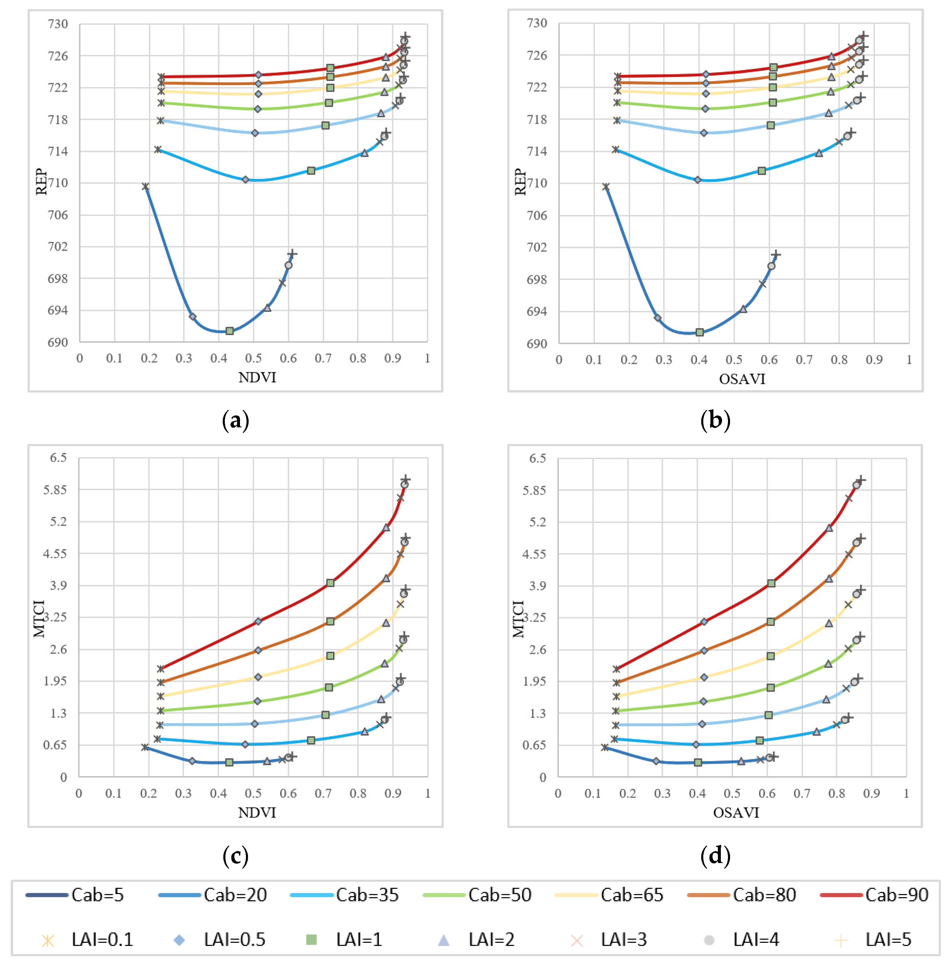
ρs on the 15 vegetation indices described above. During the sensitivity analysis process, only the interference factor was varied according to the threshold range and the remained parameters of PROSAIL model were set to the fixed value. The VI combinations were drawn in a two-VI space, as shown in Figure 2.
In Figure 2, the LAI isolines (the same symbol) and the Cab isolines (the same color) had different trends. This indicates that the LAI and Cab can be well-separated by VI combinations. In general, the sensitivity of VI combinations changed with the LAI and Cab, varying in different VI spaces and positions. The VI combinations of NDVI–MTCI and OSAVI–MTCI had higher discreteness (the Cab isolines in these VI spaces were the most separated) and are better for distinguishing Cab, indicating the most sensitivity. Due to the saturation effects, the higher the LAI value, the lower the sensitivity of the VI combinations to LAI and the more dense the LAI isolines in two-VI space. When both the LAI and Cab were high, the saturation effect was most pronounced.
It was difficult to directly judge the dispersion of VI combination only from the figure. Therefore, the ability of different combinations to distinguish LAI or Cab was quantitatively described based on the distance of adjacent points in the matrix. The operations were as follows: (1) Normalize the matrix; (2) Calculate the mean value (Lave) and standard deviation (Lstd) of the distance between different Cab points on the LAI isoline to represent the dispersion of the current matrix to Cab. The larger the Lave, the better the dispersion of the matrix to Cab, and the smaller the Lstd, the better the stability of the matrix. Similarly, the distance mean and variance of LAI on Cab isolines were also calculated. The larger the Lave of LAI, the better the dispersion of the matrix for LAI, and the smaller the Lstd of LAI, the better the stability of the matrix.
As shown in Table 7, for Cab, OSAVI–MTCI not only had the highest dispersion (Lave of Cab was 0.0931) but also the lowest standard deviation (Lstd of Cab was 0.0285), which was consistent with the phenomenon described above. For LAI, OSAVI–REP performed best, but at the same time, it had certain instability for Cab. It can also be seen from Figure 2 that in the OSAVI–REP space, contour lines such as Cab = 5 μg/cm2, 20 μg/cm2, 35 μg/cm2 were relatively discrete, while contour lines such as Cab = 65 μg/cm2, 80 μg/cm2, 90 μg/cm2 were relatively clustered. This indicates that the degree of dispersion variability of this VI combination is relatively large (Lstd of Cab was 0.0888). Thus, a partitioned multi-stage inversion strategy should be established for joint estimation of LAI and Cab. For example, the Cab parameter should be preferentially retrieved because its VI combinations were more sensitive to Cab.
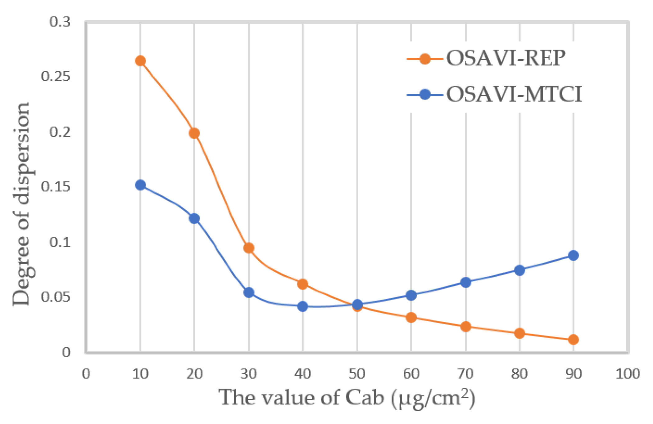
The dispersion of OSAVI–REP to Cab under different thresholds was further analyzed to determine the combination mode of the two VI matrices. It can be seen from Figure 3 that the dispersion degree of OSAVI–REP decreases significantly with the increase in Cab value. Therefore, it is necessary to introduce the VI matrix in stages according to the variation trend of the dispersion. That is, OSAVI–REP should be used when the Cab is low, while OSAVI–MTCI should be used when the Cab is high.
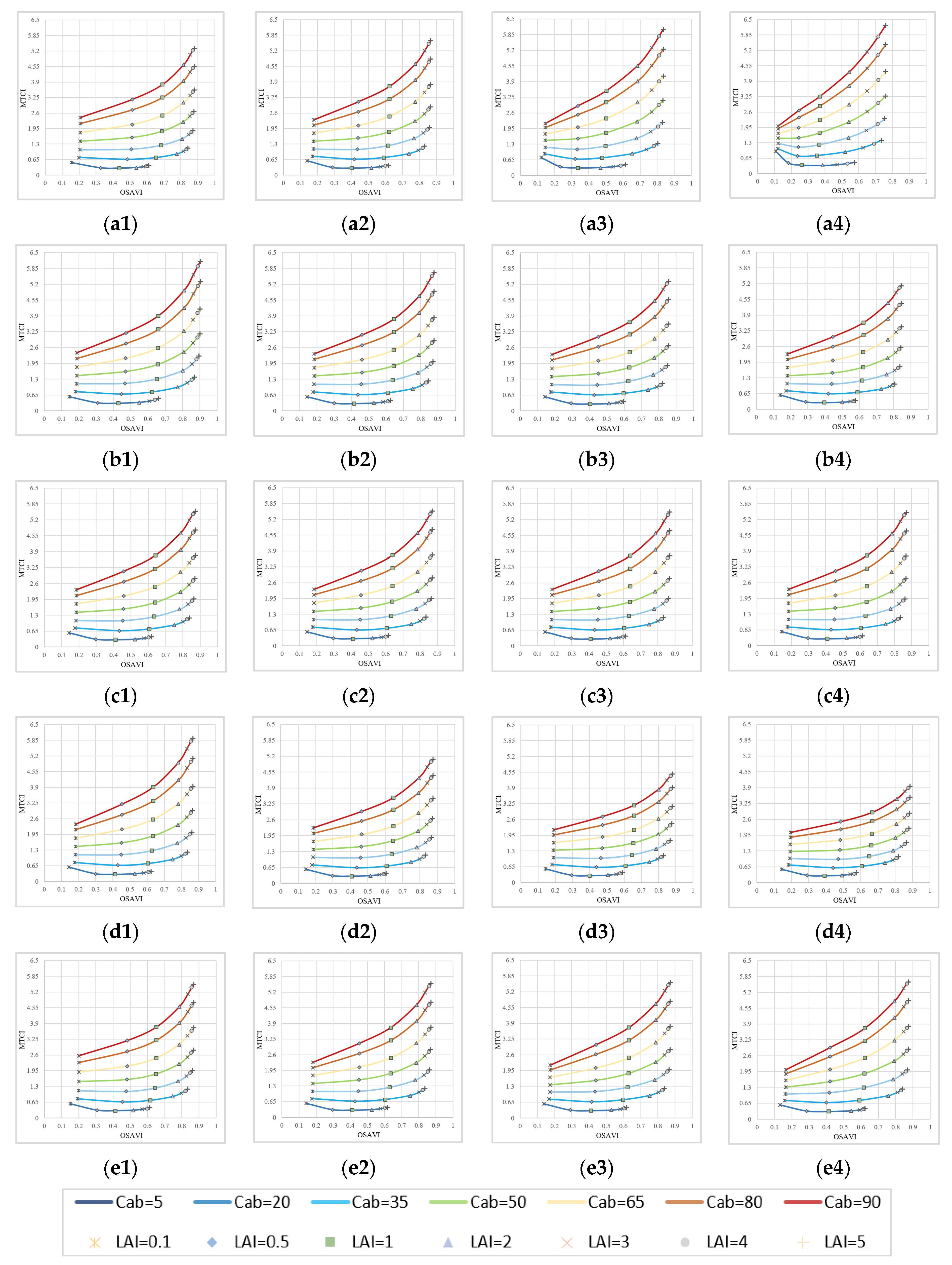
The effects of the other parameters on VI combinations are also evaluated in this paper. Taking VI combination OSAVI–MTCI as an example, its sensitivity to the parameters of ALA, Cm, Cw, N and ρs was analyzed using the simulations of PROSAIL. The results are shown in Figure 4. By comparing the curves in Figure 4 with those of the curves in Figure 2, the variation in Cm, Cw and ρs had no obvious effect on the results. The changes in ALA and N had limited effects on OSAVI–MTCI combination, for which N had a relatively high impact; the parameter ALA had a great influence on LAI when LAI value was low (Figure 4(a1)–(a4)), but it did little to change the overall properties of OSAVI–MTCI combination. Although the effect of N on Cab was minimal when the Cab value was lower than 35 μg/cm2 (Figure 4(d1)–(d4)), it led to a reduction in the dispersion of OSAVI–MTCI combination (the Cab curves were relatively gathered).

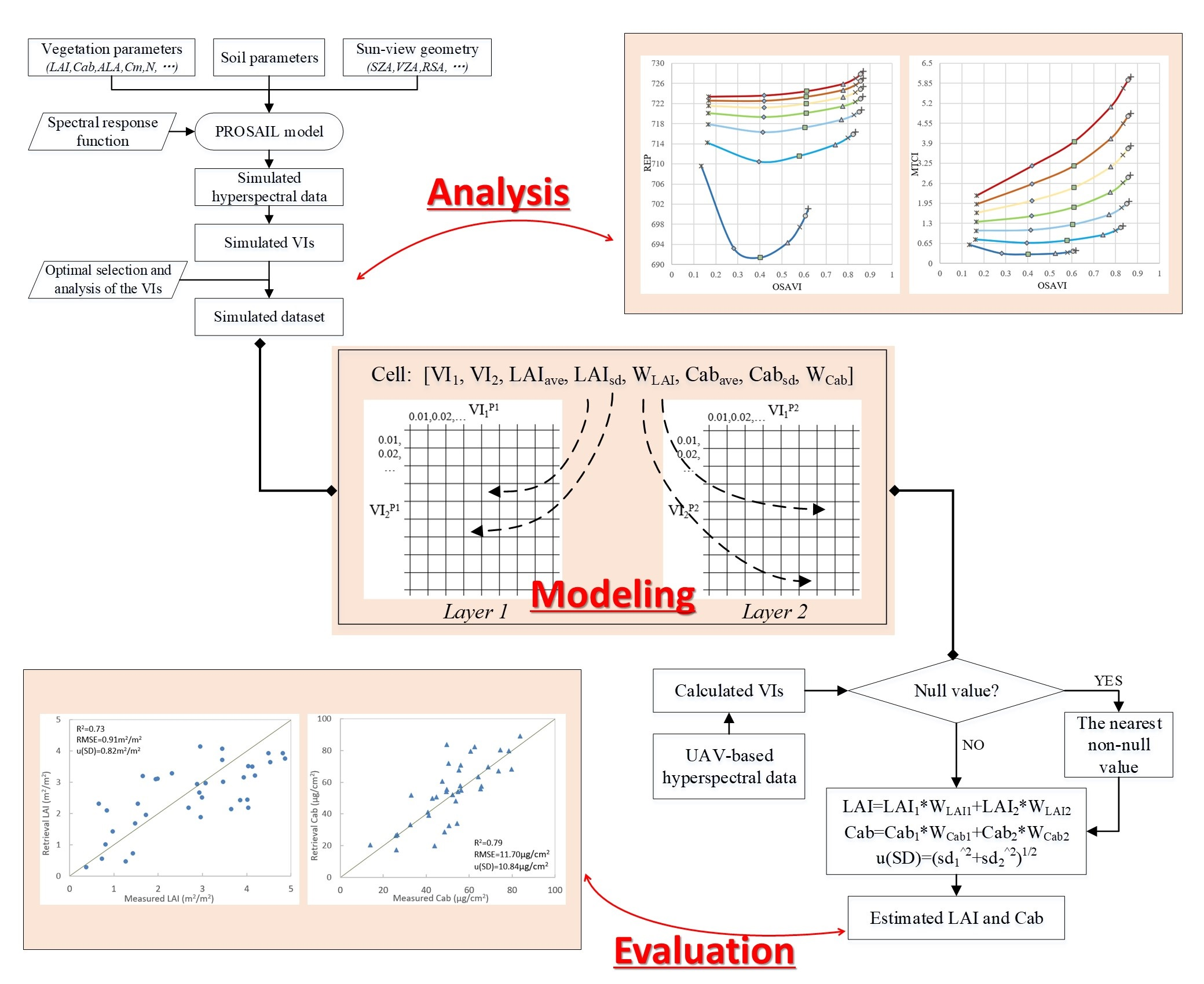
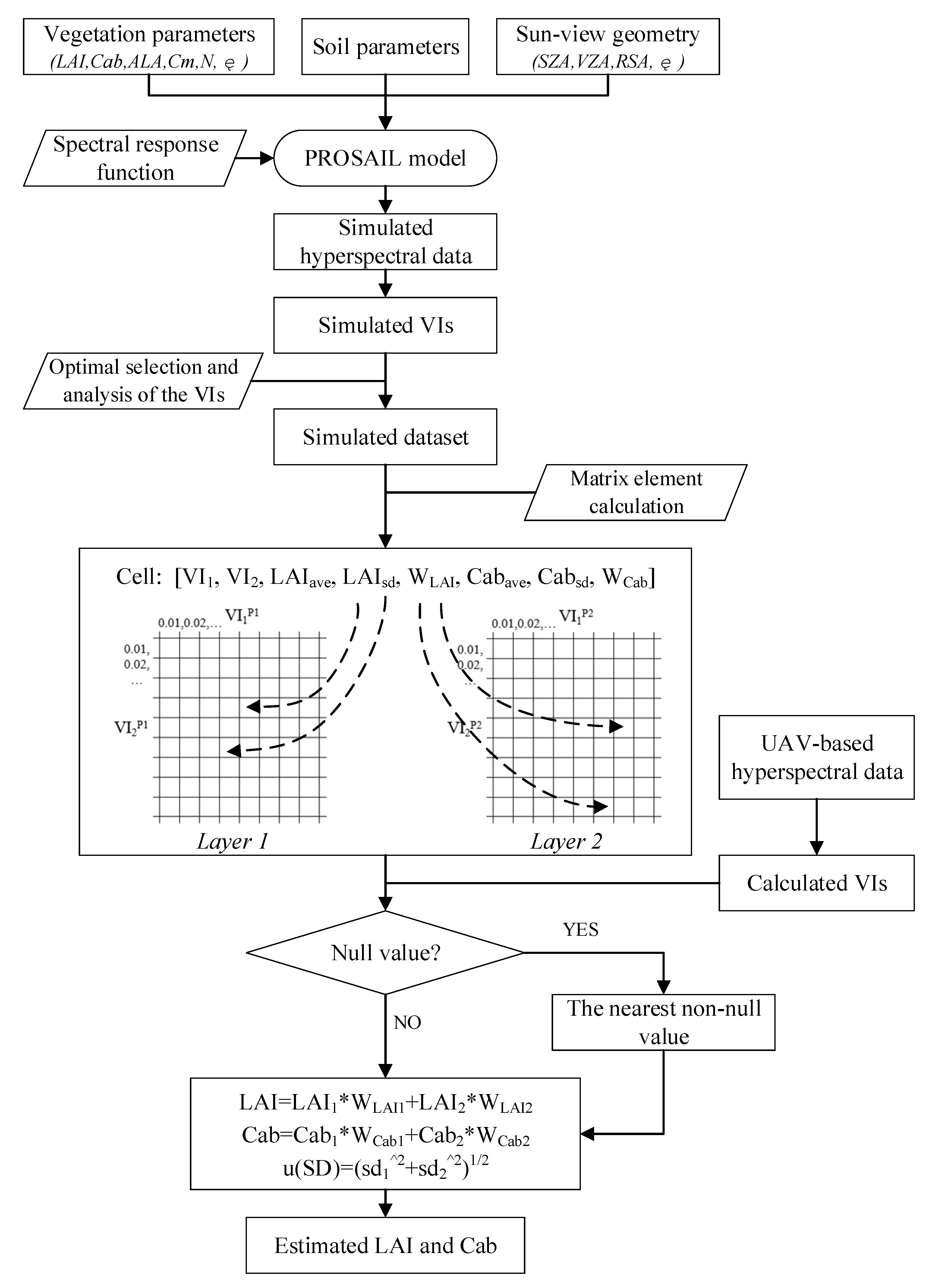
2.2.4. Establishment of a Two-Layer Matrix Inversion Method

As shown in Figure 5, the VI combinations of OSAVI–REP and OSAVI–MTCI were divided into cells to establish the inversion matrix. Each matrix had 1000 × 1000 cells and each cell corresponded to a small range of vegetation index values. Based on the modeling dataset simulated from the PROSAIL model, the LAI and Cab values were assigned to a matrix cell according to the values of the two simulated VIs. Because one cell had multiple values of LAI and Cab, all the values mapped to the same cell would be calculated as average and standard deviation. Then, the average (ave) and standard deviation (sd) values of the LAI and Cab were mapped to each cell, constituting the average and standard deviation matrices.
The distribution of matrix dispersion was uneven due to the value change of LAI and Cab, which was described in Section 2.2.3. The dispersion curves of OSAVI–REP matrix and OSAVI–MTCI matrix converge at Cab ≈ 50 μg/cm2 (Figure 3). When Cab was low, OSAVI–REP matrix had better discretization, which should be used for Cab estimation. Otherwise, OSAVI–MTCI should be used for Cab estimation. In order to reduce the error brought by the instability of the dispersion of the matrix, the range (40 μg/cm2, 60 μg/cm2) was determined as the intermediate choice. Then, the weight coefficient can be established to determine the participation of matrix cells in different layers. As described above, when Cab value ≤ 40 μg/cm2, OSAVI–REP dispersion was high. Therefore, the corresponding cell in OSAVI–REP matrix should be assigned a higher weight, which was set to 1 in this paper. Similarly, when Cab value > 60 μg/cm2, OSAVI–MTCI dispersion was high and the corresponding cell in OSAVI–MTCI should be assigned a higher weight. When 40 μg/cm2 < Cab value ≤ 60 μg/cm2, the corresponding cell in OSAVI–REP matrix and OSAVI–MTCI matrix were both assigned as 0.5. At last, the weight coefficient (w) was entered in each cell to form the weight matrix.
In the retrieval process, the expected estimation value of LAI and Cab were calculated based on the average matrix and the weight matrix. Additionally, the total standard deviation represented the inversion uncertainty.
After establishing the two-layer matrix, the LAI and Cab can be easily retrieved based on the four VIs calculated from the reflectance data. If the cell value of each layer matrix was valid, its value can be calculated with the weight coefficient and set as the estimated LAI and Cab. However, in some cases, the VIs calculated from the remotely sensed data were not within the range of the matrix and LAI and Cab values of the corresponding units could not be searched. In other words, the VI combinations calculated based on simulated reflectance data still cannot cover those calculated based on the remotely sensed data. This could be due to improper parameter settings during PROSAIL model simulation or the observation deviation of remotely sensed data. If the searched LAI and Cab values in the located cell were both null in two-layer matrices, the nearest 8-connected neighborhood was averaged and used as the estimated LAI and Cab. If the values of LAI and Cab in the located cell were null only in a one-layer matrix, the non-null values of the other layer were directly set to the estimated LAI and Cab.

2.2.5. Joint Estimation of LAI and Cab

The joint estimation of LAI and Cab included two cases:
Case 1 based on simulated data: the simulated test datasets were used for retrieving LAI and Cab through VI empirical model, the single-layer VI matrix and the two-layer matrix.
As described in Section 2.2, 50,000 canopy spectra were used as a test dataset (TD data) for joint estimation of LAI and Cab. In this case, to further consider bias in the acquisition and processing of remote sensing data, a new test dataset (NTD data) was constructed by adding 5% relative Gaussian noise to the canopy spectra as reflectance uncertainty. The new test dataset was produced, which can also be used for evaluating the influence of reflectance measurement uncertainty on the retrieval accuracy of vegetation parameters.
Therefore, in this case, the two-layer matrix was evaluated by retrieving LAI and Cab from the simulated data with and without noise.
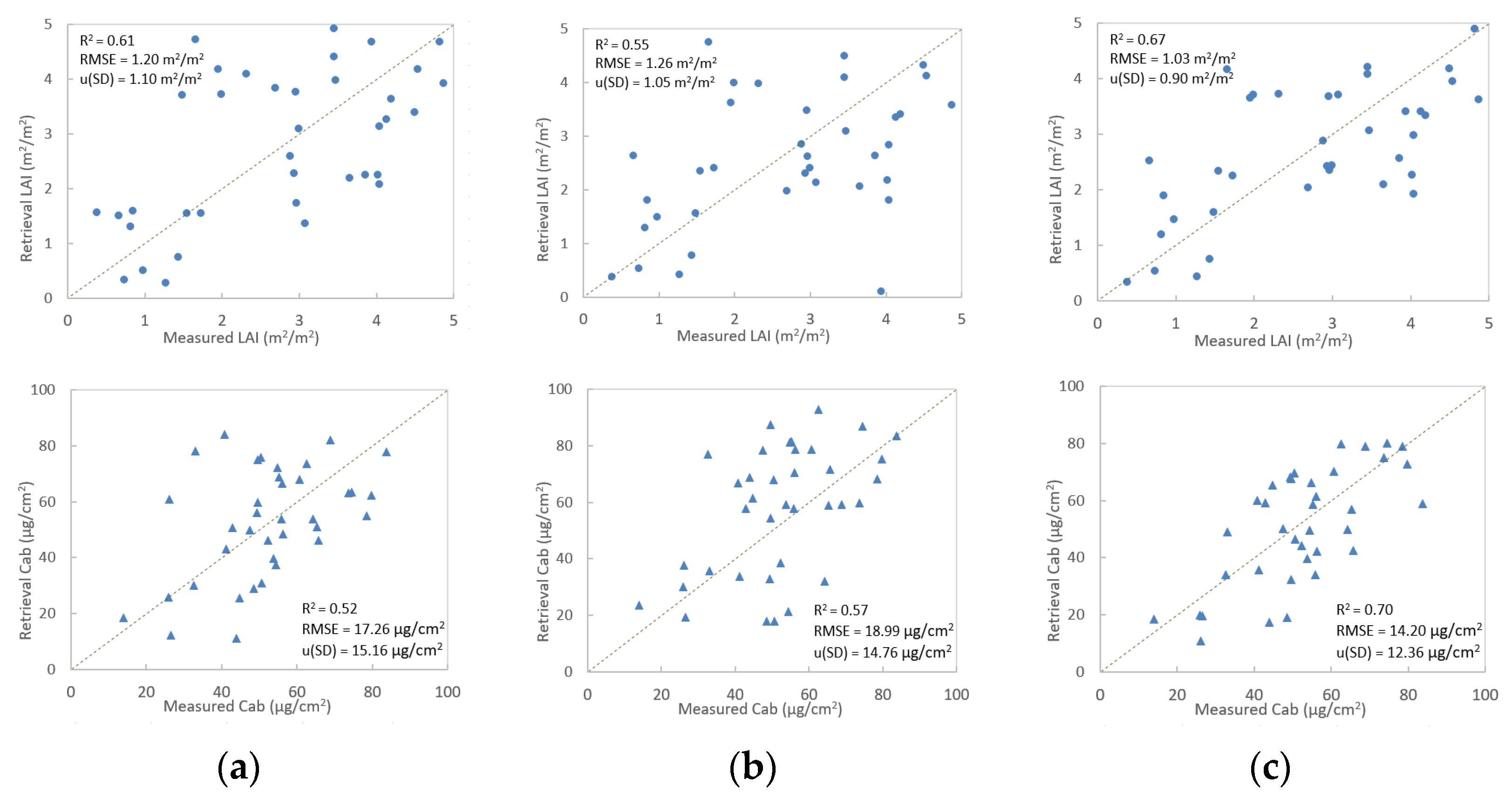
Case 2 based on UAV hyperspectral data: the UAV hyperspectral data obtained during the field campaign were used for retrieving LAI and Cab through approaches of matrices and machine learning, including the single-layer matrix of OSAVI–REP, the single-layer matrix of OSAVI–MTCI, the two-layer matrix, partial least squares regression (PLSR) and random forest (RF).
In Case 2, to improve the model robustness when the model was used for actual observation data, the two-layer matrix was optimized by adding 5% relative Gaussian noise for comparison. Therefore, in this case, the two-layer matrix established with and without noise was evaluated by retrieving LAI and Cab from the UAV hyperspectral data.

3. Results

3.1. Evaluation of the Two-Layer Matrix Based on Simulated Data

Based on the two-layer matrix, LAI and Cab were jointly estimated from the simulated TD and NTD datasets. The inversion results were compared with those estimated using the VI empirical model and the single-layer VI matrix (Table 8). The following statistical indicators were used for accuracy analysis: coefficient of determination (R2) and root mean square error (RMSE). The standard deviation (u(SD)) characterized the performance of the matrices and was also used to represent the uncertainty of LAI and Cab estimation.
As shown in Table 8, regardless of whether the test dataset contains noise, the two-layer retrieval matrix achieved the best estimation accuracies of the LAI and Cab. LAI retrieved from NTD (TD) data obtained R2 of 0.76 (0.79) and RMSE of 0.92 m2/m2 (0.87 m2/m2). Cab retrieved from NTD (TD) data obtained R2 of 0.79 (0.85) and RMSE of 12.66 μg/cm2 (11.05 μg/cm2). Although the single-layer matrix of OSAVI–REP had similar estimated accuracy for retrieving LAI from the simulated reflectance with and without reflectance noise, for Cab estimation, the two-layer matrix of OSAVI–REP and OSAVI–MTCI performed better. In addition, compared with the single-layer matrix of OSAVI–REP, the uncertainty of the two-layer matrix applied to Cab estimation was lower. The reason why the two-layer matrix was superior to the single-layer matrix was that the two-layer matrix was combined with the most separable part of the single-layer matrix, which reduced the cross-influence of LAI and Cab and improved the robustness of the inversion process.
Compared with the empirical model, the matrix-based approaches were obviously more accurate for estimating LAI and Cab. By combining OSAVI–REP and OSAVI–MTCI matrices, the two-layer matrix achieved a higher estimation than one-dimensional relationships. Retrieval results based on matrix models were better because the matrices better characterize the relationship between reflectance and LAI and Cab. Empirical models based on VI cannot represent the complex relationship between reflectance and LAI and Cab well.
The accuracy of LAI and Cab retrieved from reflectance data containing noise were significantly lower than that from the reflectance data without noise. The result indicates that the uncertainty of remotely sensed observations had an important effect on the estimation accuracy of vegetation parameters.

3.2. Evaluation of the Two-Layer Matrix Based on UAV Hyperspectral Data

The retrieval methods were applied to the UAV hyperspectral data for retrieving the grassland LAI and Cab. Figure 6 shows the results retrieved from UAV hyperspectral data based on different inversion matrices. The statistical parameters of R2, RMSE and u(SD) were used for estimation accuracy and uncertainty analysis.
Among the three inversion matrices of single-layer matrix of OSAVI–REP, single-layer matrix of OSAVI–MTCI and two-layer matrix of OSAVI–REP and OSAVI–MTCI, the estimation using the two-layer matrix yielded the highest accuracy and lowest uncertainty. The R2, RMSE and u(SD) for LAI were 0.67, 1.03 m2/m2 and 0.9 m2/m2 (Figure 6c top). The R2, RMSE and u(SD) for Cab were 0.70, 14.2 μg/cm2 and 12.36 μg/cm2 (Figure 6c bottom). The matrix of OSAVI–MTCI had the lowest accuracy for LAI estimation, with R2 = 0.55 and RMSE = 1.26 m2/m2 (Figure 6a top). The matrix of OSAVI–REP had the lowest accuracy for Cab, with R2 = 0.52 and RMSE = 17.26 μg/cm2 (Figure 6a top).
As described in Section 3.1, retrieval accuracy is influenced by the uncertainty of canopy reflectance. Therefore, the matrices were optimized by adding noise for comparison. The performance of the matrices with reflectance noise was also analyzed based on the values of mean standard deviation (u(SD)), which was also used to represent the uncertainty of LAI and Cab estimation when using those approaches. Table 9 shows that the uncertainty of the matrix did not increase significantly after the addition of simulated noise.
The optimized two-layer matrix was applied to UAV hyperspectral data for retrieving the grassland LAI and Cab. The retrieval results were compared with the single-layer matrix of OSAVI–REP and the single-layer matrix of OSAVI–MTCI, as shown in Table 10. In order to evaluate the applicability of the two-layer matrix more comprehensively, partial least squares regression (PLSR) and random forest (RF) were also selected for comparison. PLSR integrates the ideas of principal component analysis, correlation analysis and multiple regression, and has great advantages in dealing with problems where the number of independent variables is much larger than the number of samples. The RF algorithm is a versatile machine learning method that has a better fitting effect for nonlinear data.
For the three inversion matrices established based on the reflectance dataset with noise, the estimation using the two-layer matrix yielded the highest accuracy and lowest uncertainty. The R2, RMSE and u(SD) for LAI were 0.73, 0.91 m2/m2 and 0.82 m2/m2. The R2, RMSE and u(SD) for Cab were 0.79, 11.7 μg/cm2 and 10.84 μg/cm2. The retrieval results of the matrices with reflectance noise were obviously better than those of matrices without noise. This indicated that, due to the influence of different factors such as imaging condition difference, land surface spatial heterogeneity, geometric registration and atmospheric correction, there were certain uncertainties in the reflectance data obtained by the UAV platform. The addition of reflectance noise improved the robustness of the two-layer matrix. In addition, the results also showed that the proposed method had better performance compared with PLSR and RF approaches.

4. Discussion

The remote sensing of LAI and Cab is challenging due to the cross-influence between them. The joint estimation approach based on a two-layer matrix proposed in this study can retrieve LAI and Cab simultaneously at the canopy level. Compared with the one-dimensional equations of individual VIs or VI ratios, matrix-based approaches can eliminate the influence of other parameters, such as leaf angle distribution, soil background, etc., as well as the cross-influence between LAI and Cab. The elimination of influencing is helpful for improving accuracy and reducing uncertainty in LAI and Cab. Compared with traditional physical modeling and machine learning methods, this approach is much simpler and more efficient.
Although the construction of vegetation indices has taken into account the influence of non-vegetation factors, such as soil background and atmosphere, it is still difficult to avoid the interaction between vegetation parameters. Therefore, in order to reduce the influence of different vegetation parameters during inversion, a variety of VI combinations are established. For example, a three-VI combination was established for calculating leaf mass per area (LMA), which takes into account the influence of leaf water content (Cw) in the SWIR region [41]. The TCARI–OSAVI combination was established for Cab retrieval from Sentinel-2 Data, which considers the influence of LAI on it [42]. However, the retrieval result of those VI combinations may still have uncertainty. In this paper, the retrieval result of LAI from UAV hyperspectral data using a single-layer matrix of OSAVI–MTCI had an R2 of 0.55, which was still a low accuracy. The interaction between LAI and Cab was one of the factors affecting the inversion effect.
The estimation results of the two-layer matrix were obviously better than those of the single-layer matrix with and without noise. The reason why the two-layer matrix was superior to the single-layer matrix was that the two-layer matrix was combined with the most separable part of each single-layer matrix. This helped to reduce the cross-influence of LAI and Cab and improved the robustness of the inversion process. In addition, other vegetation and environmental parameters still affected the VI combinations and two-layer matrix. As shown in Section 2.2.3, parameters such as N, Cm and ALA had large effects on LAI and Cab estimation based on OSAVI–MTCI combination. A priori information can be used to limit the physical boundary of these parameters during simulation, so as to reduce the uncertainties [26].
Since the reflectance data are obtained after payload calibration, atmospheric correction and other processes, there is some uncertainty in the reflectance data. Therefore, the influence of reflectance measurement uncertainty on inversion was tested by adding or not adding noise tested in this study. If no noise was added during matrix modeling, the estimation accuracies of LAI and Cab retrieved from data with noise will be greatly reduced, as shown in Section 3.1. This showed that the uncertainty of the remotely sensed data can increase the uncertainty of retrieved LAI and Cab. If the phenomena of the same object with a different spectrum and the same spectrum with a different object were considered, noise was added in matrix modeling (namely the influence of LAI and Cab changes on reflectance). That is, the value in each cell of the matrix fluctuated within the noise range of 5% to generate mean value and standard deviation, which not only solved the ill-posed problem of physical model inversion, but also presented the uncertainty of the inversion.
The experiment for the joint estimation of the LAI and Cab from the simulated reflectance and UAV hyperspectral data both demonstrated that a two-layer matrix achieved better accuracies than the one-dimensional relationships of VIs and a single-layer matrix. Compared with machine learning methods such as RF and PLSR, the proposed method performed better, too. As a method similar to look-up table, the two-layer matrix can be used directly for LAI and Cab inversion without the need for prior measurements for training.

5. Conclusions

This paper proposed a novel approach for joint estimation of LAI and Cab using a two-layer matrix based on PROSAIL simulations. In this approach, LAI and Cab were directly obtained from a cell of the matrices, avoiding the possible distortion caused by the regression relationships of the VIs with LAI and Cab. This retrieval also reduced the cross-influence between LAI and Cab.
In this paper, the effectiveness of the approach for joint estimation of LAI and Cab was examined using simulated data and UAV hyperspectral data. Compared with the traditional single VIs and single-layer matrices, the two-layer matrix estimated LAI and Cab simultaneously, which improved inversion efficiency and accuracy. The results of adding noise showed that the simulation effect can be improved by considering the influence of noise when constructing the matrix. The accuracy of LAI and Cab retrieval from UAV hyperspectral data was significantly improved; the RMSE was reduced from 1.03 m2/m2 to 0.91 m2/m2 for LAI, and from 14.2 μg/cm2 to 11.7 μg/cm2 for Cab.

Author Contributions

Conceptualization, X.Z.; methodology, X.Z. and Q.Y.; software, X.Z. and X.C.; validation, X.Z. and Q.Y.; formal analysis, X.Z. and Q.Y.; investigation, X.Z., Q.Y. and Z.D.; resources, X.Z. and X.C.; data curation, X.Z. and Z.D.; writing—original draft preparation, X.Z. and Q.Y.; writing—review and editing, X.Z., Q.Y., X.C. and Z.D.; visualization, X.Z. and X.C.; supervision, X.Z.; project administration, X.Z.; funding acquisition, X.Z. All authors have read and agreed to the published version of the manuscript.

Funding

This research was funded by the National Key Research and Development Program of China (2022YFB3903501), the Major Science and Technology Projects of the Inner Mongolia Autonomous Region (2021ZD0044), the Strategic Pilot Science and Technology Project of Chinese Academy of Sciences (XDA26010203) and the Future-Star program of the Aerospace Information Research Institute (E2Z106010F).

Data Availability Statement

Not applicable.

Acknowledgments

We thank all field staff for providing measurement data support for the study, as well as the open access to the PROSAIL model.

Conflicts of Interest

The authors declare no conflict of interest.

Abbreviations

AbbreviationReference
LAILeaf area index
CabLeaf chlorophyll a+b content
UAVUnmanned aerial vehicle
PROSAILPROSPECT+SAIL
PROSPECTPROperties SPECTra
SAILScattering by Arbitrarily Inclined Leaves
VIsVegetation indices
R2The coefficient of determination
RMSERoot mean square error
u(SD)Standard deviation
LUTLook-up table
NNNeural Network
SASimulated Annealing
GAGenetic Algorithm
PLSRPartial Least Squares Regression
RFRandom Forest
IMGERSInner Mongolia Grassland Ecosystem Research Station
HSIHyperspectral imaging
FOVField of view
WGS 84World Geodetic System 1984
UTMUniversal Transverse Mercator
PVCPolyvinyl chloride
CmDry matter content
CwEquivalent water thickness
ALAAverage leaf angle
NLeaf structure parameter
HotHot-spot size parameter
fSoil factor
ρsSoil reflectance
VZAView zenith angle
SZASun zenith angle
RSARelative azimuth angle
NDVINormalized difference vegetation index
SRSimple ratio vegetation index
EVIEnhanced vegetation index
MTVIMulti temporal vegetation index
OSAVIOptimized soil-adjusted vegetation index
MSAVIModified soil-adjusted vegetation index
TCARITransformed chlorophyll absorption ratio index
MCARIModified chlorophyll absorption ratio index
MTCIModified triangular chlorophyll index
CIgreenGreen chlorophyll index
CIrededgeRed-edge chlorophyll index
REPRed edge position
LMALeaf mass per area

References

  1. Chen, J.M.; Black, T.A. Defining leaf area index for non-flat leaves. Plant Cell Environ. 1992, 15, 421–429. [Google Scholar] [CrossRef]
  2. Xu, X.; Lu, J.; Zhang, N.; Yang, T.; He, J.; Yao, X.; Cheng, T.; Zhu, Y.; Cao, W.; Tian, Y. Inversion of rice canopy chlorophyll content and leaf area index based on coupling of radiative transfer and Bayesian network models. ISPRS J. Photogramm. 2019, 150, 185–196. [Google Scholar] [CrossRef]
  3. Houborg, R.; Anderson, M.C.; Daughtry, C.S.T.; Kustas, W.P.; Rodell, M. Using leaf chlorophyll to parameterize light-use-efficiency within a thermal-based carbon, water and energy exchange model. Remote Sens. Environ. 2011, 115, 1694–1705. [Google Scholar] [CrossRef]
  4. Jin, X.; Liu, S.; Frédéric, B.; Matthieu, H.; Alexis, C. Estimates of plant density of wheat crops at emergence from very low altitude UAV imagery. Remote Sens. Environ. 2017, 198, 105–114. [Google Scholar] [CrossRef]
  5. Yue, J.; Feng, H.; Jin, X.; Yuan, H.; Li, Z.; Zhou, C.; Yang, G.; Tian, Q. A Comparison of Crop Parameters Estimation Using Images from UAV-Mounted Snapshot Hyperspectral Sensor and High-Definition Digital Camera. Remote Sens. 2018, 10, 1138. [Google Scholar] [CrossRef]
  6. Oliveira, R.A.; Tommaselli, A.M.G.; Honkavaara, E. Generating a hyperspectral digital surface model using a hyperspectral 2D frame camera. ISPRS J. Photogramm. 2019, 147, 345–360. [Google Scholar] [CrossRef]
  7. Duan, B.; Liu, Y.; Gong, Y.; Peng, Y.; Wu, X.; Zhu, R.; Fang, S. Remote estimation of rice LAI based on Fourier spectrum texture from UAV image. Plant Methods 2019, 15, 124. [Google Scholar] [CrossRef]
  8. Zarco, P.J.; Hornero, A.; Peck, P.S.A.; Kattenborn, T.; Kempeneers, P.; Hernández-Clemente, R. Chlorophyll content estimation in an open-canopy conifer forest with Sentinel-2A and hyperspectral imagery in the context of forest decline. Remote Sens. Environ. 2019, 223, 320–335. [Google Scholar] [CrossRef]
  9. Zhu, X.H.; Li, C.R.; Tang, L.L. Look-up-table approach for leaf area index retrieval from remotely sensed data based on scale information. Opt. Eng. 2018, 57, 033104. [Google Scholar] [CrossRef]
  10. Sanjiv, K.S.; Hitendra, P.; Anindita, D.; Jochem, V.; Juan, P.R. Estimation of leaf area index using PROSAIL based LUT inversion, MLRA-GPR and empirical models: Case study of tropical deciduous forest plantation, North India. Int. J. Appl. Earth Obs. 2020, 86, 102027. [Google Scholar]
  11. Sun, B.; Wang, C.; Yang, C.; Xu, B.; Zhou, X.; Xie, J.; Xu, S.; Liu, B.; Xie, T.; Kuai, J.; et al. Retrieval of rapeseed leaf area index using the PROSAIL model with canopy coverage derived from UAV images as a correction parameter. Int. J. Appl. Earth Obs. 2021, 102, 102373. [Google Scholar] [CrossRef]
  12. Baret, F.; Buis, S. Estimating canopy characteristics from remote sensing observations. Review of methods and associated problems. In Advances in Land Remote Sensing: System, Modeling, Inversion and Application; Liang, S., Ed.; Springer: Dordrecht, The Netherlands, 2008; pp. 172–301. [Google Scholar]
  13. Yan, G.; Mu, X.; Ma, Y.; Li, Z. A strategy to integrate a priori knowledge for an improved inversion of LAI from BRDF modelling. Int. J. Remote Sens. 2008, 29, 4927–4941. [Google Scholar] [CrossRef]
  14. Zhu, X.H.; Li, C.R.; Zhang, Z.W.; Zhou, Y.S. Multi-scale, multi-stage inversion method for retrieval of LAI. In Proceedings of the 2015 IEEE International Geoscience and Remote Sensing Symposium (IGARSS), Milan, Italy, 26–31 July 2015. [Google Scholar]
  15. Liang, L.; Di, L.; Zhang, L.; Deng, M.; Qin, Z.; Zhao, S.; Lin, H. Estimation of crop LAI using hyperspectral vegetation indices and a hybrid inversion method. Remote Sens. Environ. 2015, 165, 123–134. [Google Scholar] [CrossRef]
  16. Haboudane, D.; Tremblay, N.; Miller, J.R.; Vigneault, P. Remote estimation of crop chlorophyll content using spectral indices derived from hyperspectral data. IEEE Trans. Geosci. Remote Sens. 2008, 46, 423–437. [Google Scholar] [CrossRef]
  17. Xu, M.; Liu, R.; Chen, J.; Liu, Y.; Shang, R.; Ju, W.; Wu, C.; Huang, W. Retrieving leaf chlorophyll content using a matrix-based vegetation index combination approach. Remote Sens. Environ. 2019, 224, 60–73. [Google Scholar] [CrossRef]
  18. Sha, Z.; Wang, Y.; Bai, Y.; Zhao, Y.; Jin, H.; Na, Y.; Meng, X. Comparison of leaf area index inversion for grassland vegetation through remotely sensed spectra by unmanned aerial vehicle and field-based spectroradiometer. J. Plant Ecol. 2019, 12, 395–408. [Google Scholar] [CrossRef]
  19. Inner Mongolia Grassland Ecosystem Research Station, Chinese Academy of Sciences. Inner Mongolia Grassland Ecosystem Research Station, Chinese Academy of Sciences. Bull. China Acad. Sci. 2017, 32, 917–918. [Google Scholar]
  20. Hyperspectral Camera. Available online: http://senop.fi/optronics-hyperspectral#hyperspectralCamera (accessed on 12 December 2022).
  21. Jacquemoud, S.; Baret, F. PROSPECT: A model of leaf optical properties spectra. Remote Sens. Environ. 1990, 34, 75–91. [Google Scholar] [CrossRef]
  22. Verhoef, W. Light scattering by leaf layers with application to canopy reflectance modeling: The SAIL model. Remote Sens. Environ. 1984, 16, 125–141. [Google Scholar] [CrossRef]
  23. Jacquemoud, S.; Verhoef, W.; Baret, F.; Bacour, C.; Zarco-Tejada, P.; Asner, G.; François, C.; Ustin, S. PROSPECT+SAIL models: A review of use for vegetation characterization. Remote Sens. Environ. 2009, 113, 56–66. [Google Scholar] [CrossRef]
  24. Zhu, X.H.; Li, C.R.; Tang, L.L.; Ma, L.L. Retrieval and scale effect analysis of LAI over typical farmland from UAV-based hyperspectral data. In Proceedings of the SPIE Remote Sensing, Strasbourg, France, 21 October 2019. [Google Scholar]
  25. Darvishzadeh, R.; Matkan, A.A.; Ahangar, A.D. Inversion of a radiative transfer model for estimation of rice canopy chlorophyll content using a lookup-table approach. Int. J. Appl. Earth Obs. 2012, 5, 1222–1230. [Google Scholar] [CrossRef]
  26. Zhu, X.H.; Feng, X.M.; Zhao, Y.S. Multi-scale MSDT inversion based on LAI spatial knowledge. Sci. China Earth Sci. 2012, 55, 1297–1305. [Google Scholar] [CrossRef]
  27. Houborg, R.; Anderson, M.; Daughtry, C. Utility of an image-based canopy reflectance modeling tool for remote estimation of LAI and leaf chlorophyll content at the field scale. Remote Sens. Environ. 2009, 113, 259–274. [Google Scholar] [CrossRef]
  28. Haboudane, D.; Miller, J.R.; Pattey, E.; Zarco-Tejada, P.; Strachan, I. Hyperspectral vegetation indices and novel algorithms for predicting green LAI of crop canopies: Modeling and validation in the context of precision agriculture. Remote Sens. Environ. 2004, 90, 337–352. [Google Scholar] [CrossRef]
  29. Rouse, J.W.; Haas, R.H.; Schell, J.A.; Deering, D.W. Monitoring Vegetation Systems in the Great Plains with ERTS. In Proceedings of the Third Earth Resources Technology Satellite-1 Symposium, NASA, Washington, DC, USA, 10–14 December 1973; pp. 309–317. [Google Scholar]
  30. Gitelson, A.A.; Merzlyak, M.N. Remote estimation of chlorophyll content in higher plant leaves. Int. J. Remote Sens. 1997, 18, 2691–2697. [Google Scholar] [CrossRef]
  31. Huete, A.; Justice, C.; Liu, H. Development of vegetation and soil indices for MODIS-EOS. Remote Sens. Environ. 1994, 49, 224–234. [Google Scholar] [CrossRef]
  32. Rondeaux, G.; Steven, M.; Baret, F. Optimization of soil-adjusted vegetation indices. Remote Sens. Environ. 1996, 55, 95–107. [Google Scholar] [CrossRef]
  33. Qi, J.; Chehbouni, A.; Huete, A.R.; Kerr, Y.H.; Sorooshian, S. A modified soil adjusted vegetation index. Remote Sens. Environ. 1994, 48, 119–126. [Google Scholar] [CrossRef]
  34. Wu, C.; Niu, Z.; Tang, Q.; Huang, W. Estimating chlorophyll content from hyperspectral vegetation indices: Modeling and validation. Agric. For. Meteorol. 2008, 148, 1230–1241. [Google Scholar] [CrossRef]
  35. Daughtry, C.S.T.; Walthall, C.L.; Kim, M.S.; de Colstoun, E.B.; McMurtrey, J.E., III. Estimating corn leaf chlorophyll concentration from leaf and canopy reflectance. Remote Sens. Environ. 2000, 74, 229–239. [Google Scholar] [CrossRef]
  36. Dash, J.; Curran, P.J. Evaluation of the MERIS terrestrial chlorophyll index (MTCI). Adv. Space Res. 2007, 39, 100–104. [Google Scholar] [CrossRef]
  37. Gitelson, A.; Vina, A.; Ciganda, V.; Rundquist, C.; Arkebauer, J. Remote estimation of canopy chlorophyll content in crops. Geophys. Res. Lett. 2005, 32, L08403. [Google Scholar] [CrossRef]
  38. Clevers, J.P.W. Imaging spectrometry in agriculture—Plant vitality and yield in dicators. In Imaging Spectrometry—A Tool for Environmental Observations; Hill, J., Mégier, J., Eds.; Springer: Dordrecht, The Netherlands, 1994; pp. 193–219. [Google Scholar]
  39. Broge, N.H.; Leblanc, E. Comparing prediction power and stability of broadband and hyperspectral vegetation indices for estimation of green leaf area index and canopy chlorophyll density. Remote Sens. Environ. 2001, 76, 156–172. [Google Scholar] [CrossRef]
  40. Haboudane, D.; Miller, J.R.; Tremblay, N.; Zarco-Tejada, P.J.; Dextraze, L. Integrated narrow-band vegetation indices for prediction of crop chlorophyll content for application to precision agriculture. Remote Sens. Environ. 2002, 81, 416–426. [Google Scholar] [CrossRef]
  41. Chen, Y.; Sun, J.; Wang, L.; Shi, S.; Gong, W.; Wang, S.; Tagesson, T. Optimized Estimation of Leaf Mass per Area with a 3D Matrix of Vegetation Indices. Remote Sens. 2021, 13, 3761. [Google Scholar] [CrossRef]
  42. Clevers, J.; Kooistra, L.; Brande, M. Using Sentinel-2 Data for Retrieving LAI and Leaf and Canopy Chlorophyll Content of a Potato Crop. Remote Sens. 2017, 9, 405. [Google Scholar] [CrossRef]
Figure 1. The study area.
Remotesensing 15 02525 g001
Figure 2. The analysis of dispersion of different VI combinations: (a) NDVI vs. REP, (b) OSAVI vs. REP, (c) NDVI vs. MTCI, (d) OSAVI vs. MTCI.
Remotesensing 15 02525 g002
Figure 3. The variation in the dispersion of different matrices with Cab.
Remotesensing 15 02525 g003
Figure 4. The sensitivity analysis of VI combinations to other parameters. (a1) ALA = 10, (a2) ALA = 25, (a3) ALA = 40, (a4) ALA = 60; (b1) Cm = 0.001, (b2) Cm = 0.004, (b3) Cm = 0.007, (b4) Cm = 0.009; (c1) Cw = 0.005, (c2) Cw = 0.017, (c3) Cw = 0.029, (c4) Cw = 0.04; (d1) N = 0.001, (d2) N = 0.004, (d3) N = 0.007, (d4) N = 0.009; (e1) ρs = 0.001, (e2) ρs = 0.004, (e3) ρs = 0.007, (e4) ρs = 0.009.
Remotesensing 15 02525 g004
Figure 5. Flowchart of the joint estimation approach for LAI and Cab.
Remotesensing 15 02525 g005
Figure 6. The retrieval of LAI (top) and Cab (bottom) from UAV hyperspectral data using different methods: (a) single-layer matrix of OSAVI–REP; (b) single-layer matrix of OSAVI–MTCI; (c) two-layer matrix of OSAVI–REP and OSAVI–MTCI.
Remotesensing 15 02525 g006
Table 1. Technical properties of the Rikola hyperspectral camera.
ParameterValue
Image modeFrame-based
FOV36.5°
Pixel resolution1010 × 1010
Field resolution6.5 cm@100 m
Spectral range500–900 nm
Spectral resolution~10 nm
Weight720 g
Table 4. The relationship between LAI and VIs.
IndicesFitting EquationabR2RMSE
NDVIf(x) = axb3.1332.0360.74420.4395
OSAVIf(x) = axb3.6331.5440.73250.4494
MTVI2f(x) = axb3.060.870.70810.4695
MSAVIf(x) = ax + b3.574−0.11350.6830.4892
EVIf(x) = ax + b3.421−0.28120.62790.5301
MTVI1f(x) = axb3.020.81210.62770.5302
TVIf(x) = axb0.16070.81040.62250.5339
SRf(x) = axb0.69150.79080.45640.6407
CIgreenf(x) = axb0.80820.52590.44490.6474
MCARIf(x) = axb3.0350.32230.43060.6557
CIrededgef(x) = axb1.9370.5990.31120.7212
TCARIf(x) = ax + b4.220.92380.18140.7862
MTCIf(x) = aexp(bx)1.0250.22560.09540.8265
TCARI2f(x) = aexp(bx)1.592−0.48360.01110.8641
REPf(x) = aexp(bx)0.00180.00930.00610.8663
Table 5. The relationship between Cab and VIs.
IndicesFitting EquationabR2RMSE
REPf(x) = axb2.142 × 10−21073.980.81048.658
MTCIf(x) = axb31.850.78570.719911.133
CIrededgef(x) = axb58.030.59380.510714.23
TCARIf(x) = ax + b−159.166.560.470414.81
CIgreenf(x) = ax + b4.72227.670.334516.6
MCARIf(x) = aexp(bx)59.5−2.0170.326516.7
SRf(x) = ax + b8.85220.570.301817
TCARI2f(x) = ax + b−71.8854.470.255917.55
NDVIf(x) = aexp(bx)35.40.35310.020820.13
TVIf(x) = aexp(bx)48.94−0.00530.009720.25
MTVI1f(x) = ax + b−8.82748.790.009320.25
EVIf(x) = aexp(bx)40.370.20290.007820.27
OSAVIf(x) = aexp(bx)40.060.20760.007220.27
MSAVIf(x) = aexp(bx)41.330.18240.006220.28
MTVI2f(x) = axb43.87−0.02260.001820.33
Table 6. The VI combinations.
↓ LAIREPMTCI
NDVI(NDVI, REP)(NDVI, MTCI)
OSAVI(OSAVI, REP)(OSAVI, MTCI)
↓ CabNDVIOSAVI
REP(REP, NDVI)(REP, OSAVI)
MTCI(MTCI, NDVI)(MTCI, OSAVI)
Table 7. The degree of dispersion of different matrices.
 NDVI–REPOSAVI–REP NDVI–MTCIOSAVI–MTCI
Lave of Cab0.08860.08490.08630.0931
Lstd of Cab0.09460.08880.03590.0285
Lave of LAI0.06940.07310.07160.0683
Lstd of LAI0.09710.08190.08960.0897
Table 8. The retrieving results from simulated data.
Retrieval MethodsPerformance
(u(SD))
TD DataNTD Data
R2RMSER2RMSE
relationships of LAI–OSAVI: y = 3.633x1.544LAI-0.691.060.581.22
relationships of Cab–REP: y = 2.142 × 10−210x73.98Cab-0.7512.630.6914.02
single-layer matrix of OSAVI–REPLAI0.870.750.940.720.99
Cab9.510.7912.240.7313.41
single-layer matrix of OSAVI–MTCILAI0.980.711.010.661.09
Cab7.930.8314.520.7716.16
two-layer matrix of OSAVI–REP and OSAVI–MTCILAI0.670.790.870.760.92
Cab7.60.8511.050.7912.66
Table 9. The uncertainty of the matrices.
Retrieval MethodsPerformance (u(SD))
single-layer matrix of OSAVI–REPLAI: 0.88, Cab: 9.34
single-layer matrix of OSAVI–MTCILAI: 1.04, Cab: 7.83
two-layer matrix of
OSAVI–REP and OSAVI–MTCI
LAI: 0.72, Cab: 7.4
Table 10. The retrieval of LAI and Cab from UAV hyperspectral data using different methods.
Retrieval MethodsRetrieval Accuracy
R2RMSE
single-layer matrix of OSAVI–REPLAI: 0.66LAI: 1.04 m2/m2
Cab: 0.61Cab: 16.82 μg/cm2
single-layer matrix of OSAVI–MTCILAI: 0.63LAI: 1.13 m2/m2
Cab: 0.69Cab: 17.43 μg/cm2
two-layer matrix of OSAVI–REP and OSAVI–MTCILAI: 0.73LAI: 0.91 m2/m2
Cab: 0.79Cab: 11.70 μg/cm2
partial least squares regression (PLSR)LAI: 0.65LAI: 1.07 m2/m2
Cab: 0.66Cab: 14.97 μg/cm2
random forest (RF)LAI: 0.68LAI: 1.06 m2/m2
Cab: 0.70Cab: 14.88 μg/cm2
Disclaimer/Publisher’s Note: The statements, opinions and data contained in all publications are solely those of the individual author(s) and contributor(s) and not of MDPI and/or the editor(s). MDPI and/or the editor(s) disclaim responsibility for any injury to people or property resulting from any ideas, methods, instructions or products referred to in the content.

