HyperSFormer: A Transformer-Based End-to-End Hyperspectral Image Classification Method for Crop Classification

Abstract

Crop classification of large-scale agricultural land is crucial for crop monitoring and yield estimation. Hyperspectral image classification has proven to be an effective method for this task. Most current popular hyperspectral image classification methods are based on image classification, specifically on convolutional neural networks (CNNs) and recurrent neural networks (RNNs). In contrast, this paper focuses on methods based on semantic segmentation and proposes a new transformer-based approach called HyperSFormer for crop hyperspectral image classification. The key enhancement of the proposed method is the replacement of the encoder in SegFormer with an improved Swin Transformer while keeping the SegFormer decoder. The entire model adopts a simple and uniform transformer architecture. Additionally, the paper introduces the hyper patch embedding (HPE) module to extract spectral and local spatial information from the hyperspectral images, which enhances the effectiveness of the features used as input for the model. To ensure detailed model processing and achieve end-to-end hyperspectral image classification, the transpose padding upsample (TPU) module is proposed for the model’s output. In order to address the problem of insufficient and imbalanced samples in hyperspectral image classification, the paper designs an adaptive min log sampling (AMLS) strategy and a loss function that incorporates dice loss and focal loss to assist model training. Experimental results using three public hyperspectral image datasets demonstrate the strong performance of HyperSFormer, particularly in the presence of imbalanced sample data, complex negative samples, and mixed sample classes. HyperSFormer outperforms state-of-the-art methods, including fast patch-free global learning (FPGA), a spectral–spatial-dependent global learning framework (SSDGL), and SegFormer, by at least 2.7% in the mean intersection over union (mIoU). It also improves the overall accuracy and average accuracy values by at least 0.9% and 0.3%, respectively, and the kappa coefficient by at least 0.011. Furthermore, ablation experiments were conducted to determine the optimal hyperparameter and loss function settings for the proposed method, validating the rationality of these settings and the fusion loss function.

1. Introduction

Agriculture forms the foundation for human survival and development. The classification of crops on large-scale agricultural land holds immense significance in various aspects, including crop monitoring, yield estimation, and post-disaster compensation statistics. In recent years, advanced scientific and technological approaches have been extensively employed in agriculture to reduce agricultural expenditure and advance scientific, precise, and intelligent farming methods [1]. Remote sensing technology, specifically hyperspectral remote sensing, has played a pivotal role in this regard. Hyperspectral images, known for containing a wealth of spectral features, have found widespread applications in agriculture and forestry, such as crop classification, geological exploration, forestry delineation, and environmental monitoring [2].

Crop classification methods using hyperspectral images involve the processing of hyperspectral data. In the realm of hyperspectral image classification, traditional methods typically follow a data processing sequence composed of image data preprocessing, feature extraction, and classification based on the extracted features. Multinomial logistic regression (MLR) and the support vector machine (SVM) are recognized as the most prominent feature extraction and classification methods in this context [3].

The advancement of deep learning technologies has led to the widespread adoption of recurrent neural networks (RNNs) for sequential tasks. Likewise, convolutional neural networks (CNNs) have demonstrated their applicability across a range of computer vision tasks. When compared to traditional machine learning approaches, CNNs offer notable advantages in terms of prediction accuracy. Moreover, traditional methods often entail stringent image acquisition requirements, resulting in considerably higher overall time costs as compared to CNN-based approaches [4].

Hyperspectral image classification shares similarities with image classification methods in computer vision. In this study, we refer to this specific approach as the hyperspectral image classification method based on image classification. This method entails partitioning the $H\times W$ hyperspectral image data into $H\times W$ image blocks, each with a predetermined size of $S\times S$, during both model training and prediction. In this context, $H$ and $W$ represent the dimensions of the hyperspectral image being classified, while $S$ denotes the predefined block size determined by the model input. Subsequently, all blocks undergo feature extraction utilizing an image classification model.

In contrast to traditional methods, this approach comprehensively leverages spatial features by predicting the class assignment of each pixel based on its neighboring blocks. However, this model exhibits high computational complexity due to repeated calculations for pixels in the same position during inference. Furthermore, methods based on image classification solely concentrate on the fixed data within the divided image blocks, overlooking the global spatial context information.

The primary objective of hyperspectral image classification is to assign a label to each pixel within the hyperspectral image, a task akin to semantic segmentation in computer vision. Consequently, certain researchers have tackled the challenge of hyperspectral image classification by enhancing traditional semantic segmentation models such as U-Net and the fully convolutional network (FCN). These improvements aim to enhance computational efficiency and achieve higher accuracy [5].

However, the majority of studies focusing on hyperspectral image classification have predominantly employed CNN and RNN approaches [6,7,8]. CNN-based methods primarily emphasize local features within the hyperspectral images themselves, overlooking the distinctive spectral features unique to hyperspectral data [9]. On the other hand, RNN approaches solely attend to the distinct spectral sequence features, lacking the ability to effectively process global sequence information due to their unidirectional nature. Furthermore, hyperspectral image data often exhibit imbalanced samples, with certain categories having significantly more instances, sometimes even tens of times more, compared to other categories [10]. In terms of sampling strategies, many methods only consider positive samples that are annotated with corresponding crop classes within the dataset. This results in a high misclassification rate for unlabeled negative samples that do not belong to any crop class. Consequently, the visualization of prediction results tends to have low quality, with unclear classification boundaries.

This paper revisits the structural characteristics of hyperspectral images, recognizing their abundant sequence features and the need to capture both local and global spatial context information. In light of this, we turn to the transformer architecture, which has gained popularity in computer vision. The main contributions of this paper are as follows:

(1)

We propose an end-to-end hyperspectral image classification method called HyperSFormer, which combines a transformer and semantic segmentation. HyperSFormer enhances the SegFormer architecture by replacing its encoder with an improved Swin Transformer while retaining the SegFormer decoder. By leveraging the powerful image and sequence processing capabilities of the transformer, we address the limitations of the traditional CNN and RNN frameworks in expressing global information entropy due to insufficient contextual information [11].

(2)

To extract detailed spectral and spatial context information more effectively from hyperspectral images, we introduce an adaptive hyperspectral image embedding method called hyper patch embedding (HPE). Prior to the input encoder, the HPE module encodes hyperspectral images into fixed-dimensional embedding vectors, which are then fed into the model’s encoder. The encoder leverages multiple levels of self-attention operations to capture image feature information at different levels. Additionally, a transpose padding upsample (TPU) module is integrated at the output of the decoder to preserve the width and height information of the image during the encoding and decoding process, ensuring end-to-end hyperspectral image classification.

(3)

To ensure the effectiveness of training, this study proposes an adaptive min log sampling (AMLS) strategy. This strategy determines the number of samples used for training by setting sampling coefficients $s$ based on the distribution of the different datasets. Additionally, during training, random flips are applied to the images in both vertical and horizontal directions, and samples are randomly selected from the training set for parameter updating, allowing for different gradients and effective training. Moreover, a novel loss function is designed that combines focal loss and dice loss, considering the distinctions between positive and negative samples, as well as between difficult and easy samples. This loss function aims to achieve efficient training and accurate classification outcomes.

The rest of the paper is organized as follows. Section 2 introduces the methods in hyperspectral image classification and describes the details of the proposed HyperSFormer, and Section 3 details the comparative results obtained on the three datasets. Next, Section 4 presents the ablation experiments and a discussion on the model design. Finally, Section 5 concludes the paper.

2. Background

In recent years, deep learning approaches have demonstrated remarkable achievements in the field of hyperspectral remote sensing. Particularly, methods based on image classification and semantic segmentation have proven successful for hyperspectral image classification. Traditional CNN-based methods have encountered limitations, prompting researchers to explore alternative approaches using the transformer architecture. Moreover, the persisting challenges of limited and unbalanced sample sizes remain significant considerations in hyperspectral image classification.

2.1. Hyperspectral Image Classification Methods Based on Image Classification

Image classification methods are widely used in computer vision analysis and offer significant advantages in terms of accuracy. Each pixel and its surrounding pixels need to be divided into a hyperspectral image block based on the block size set by the model before classification to enable feature extraction and model training. Zhong et al. [12] proposed the spectral–spatial residual network (SSRN) that directly uses original three-dimensional (3D) cubes as input to learn discriminative features from spectral features and spatial contexts in hyperspectral images. Ma et al. [13] introduced a double-branch multi-attention mechanism (DBMA) network, which applies two types of attention mechanisms to extract spectral and spatial features separately, ensuring the extraction of more discriminative features. Song et al. [14] developed a deep feature fusion network (DFFN) that incorporates residual learning to optimize multiple convolutional layers as identity maps, simplifying the training of deeper networks. The long short-term memory (LSTM), as a special deep learning architecture, is highly capable of modeling in the spectral dimension. Hu et al. [9] introduced the spatial–spectral convolutional LSTM 3D neural network (SSCL3DNN), which utilizes data blocks within a local sliding window as input for each storage unit, leveraging the capabilities of long short-term memory (LSTM) in modeling the spectral dimension.

Despite the remarkable classification accuracy achieved by these image classification methods, computational redundancy and the lack of global information learning in overlapping parts of adjacent blocks are inevitable. This is due to the requirement of dividing hyperspectral images into image blocks for model training.

2.2. Hyperspectral Image Classification Methods Based on Semantic Segmentation

Semantic segmentation is a fundamental task in computer vision, sharing similarities with hyperspectral image classification by assigning a classification label to each pixel in an image. Long et al. [15] introduced the FCN, the first deep learning model utilized for semantic segmentation, which achieved remarkable success in the field by replacing the final fully connected layer of the image classification model with a 1 × 1 convolutional kernel and upsampling the image to the original size for segmentation output. Ronneberger et al. [16] extended semantic segmentation to the medical domain and proposed U-Net, which integrates feature maps from different layers to capture varying sizes of information within an image. With the increasing popularity of the transformer architecture in computer vision, it has also been applied to semantic segmentation. Xie et al. [17] put forward SegFormer, a semantic segmentation network consisting of a transformer-based encoder and a multilayer perceptron (MLP)-based decoder. It adopts the architecture of the transformer block in the vision transformer (ViT), improves the downsampling method to generate feature maps of different levels, and designs a more suitable lightweight decoder of transformer architecture designed to obtain a good segmentation effect with only a four-MLP architecture.

Although the goal of hyperspectral image classification is the same as semantic segmentation, it is infeasible to transfer the semantic segmentation model directly to hyperspectral image classification. Because of the difficulty of hyperspectral image acquisition, the dataset often has only one image, and the training samples are selected based on the whole image, resulting in highly sparse training samples. The irregularity of the spectral bands of each hyperspectral image dataset also leads to model input uncertainty.

To solve the above problem, Xu et al. [18] suggested a spectral–spatial fully convolutional network (SSFCN) and a new mask matrix to assist in training for the sparse training samples of hyperspectral images. Zheng et al. [19] proposed a fast patch-free global learning (FPGA) framework for hyperspectral image classification. The sampling strategy global stochastic stratified (GS2) transforms all training samples into stratified samples to solve the problem of the failure to converge during training. Moreover, in the design of the network, FPGA applies a spectral attention encoder based on the FCN with the addition of a lateral connection module to maximize the exploitation of the global spatial context information and can effectively improve model performance.

The sampling strategy of FPGA only focuses on the stratified samples during each training instance and does not balance the relationship between difficult and easy samples. When the sample data are unbalanced, it is challenging for FPGA to extract the most discriminative features. Addressing the problem of insufficient and imbalanced hyperspectral image samples, Zhu [5] designed the spectral–spatial-dependent global learning framework (SSDGL). The framework uses a hierarchically balanced (H-B) sampling strategy and weighted softmax loss to solve the sample imbalance problem while introducing the global convolutional long short-term memory (GCL) and global joint attention mechanism (GJAM) modules to extract the long short-term dependency of spectral features and feature representations in attention regions.

Niu et al. [20] propose a novel semantic segmentation model (HSI-TransUNet) for crop mapping, which could make full use of the abundant spatial and spectral information of UAV HSI data simultaneously. The proposed HSI-TransUNet designed a spectral-feature attention module for spectral features aggregation in the encoder, and sub-pixel convolutions are adopted to avoid the chess-board effect in the segmentation results in the decoder. The proposed HSI-TransUNet has achieved good performance in crop classification. The 3D-CSAM-2DCNN proposed by Meng et al. [21] automatically learned the spectral and spatial features of 14 rice varieties and deeply extracted them by u hybrid convolutional neural network structure. The 3D-CSAM-2DCNN attempts to optimize the model with the end-to-end trainable attention module and performed the best on the fine classification of rice varieties.

2.3. Current Research on the CNN and Transformer

The CNN, as a current mainstream deep learning architecture, has the powerful ability to extract local spatial information from hyperspectral images. However, CNNs encounter performance bottlenecks due to the difficulty of the CNN architecture to capture the spectral sequence information in hyperspectral images well, especially the global spectral similarity information. The CNN can focus too much on the spatial context information in the data, distorting the order of spectral feature learning and increasing the difficulty of mining complete spectral information.

Vaswani et al. [11] found that the transformer architecture demonstrates powerful performance in natural language processing (NLP) tasks. Dosovitskiy et al. [22] reflected on the use of the transformer architecture in NLP tasks and proposed the ViT, the first computer vision model based on the transformer architecture, which performed well in vision tasks.

In the application of hyperspectral image classification, Hong et al. [23] observed the impressive capability of the transformer architecture in processing sequence information. To leverage this, they introduced a novel network for image classification known as SpectralFormer, which utilizes the transformer’s ability to learn local spectral sequence information from adjacent bands and generate group-wise spectral embeddings. Additionally, they designed a cross-layer skip connection to enable the transfer of memory-like components from shallow to deep layers through adaptive learning, effectively integrating the “soft” residuals across layers.

Nevertheless, the transformer architecture has the following drawbacks in the hyperspectral image classification methods based on semantic segmentation:

(1)

The transformer architecture performs well in processing global sequence context information. However, it is inferior to the CNN in processing local spatial information, and each encoder in the ViT model outputs a feature map of the same size, which does not consider the multiscale features of the image and cannot be used directly as an encoder in semantic segmentation [24].

(2)

The model based on the transformer architecture has strong generalization after training. However, training the model with the transformer architecture often requires numerous training samples for good generalization. The small number of training samples and the unbalanced distribution of samples in hyperspectral image classification datasets make it difficult to train the model. A sampling strategy and training scheme must be fully adapted to the transformer architecture to obtain better results [25].

2.4. Current Research on Insufficient and Imbalanced Samples

Hyperspectral image datasets are often limited to a single image, posing significant challenges to achieving high accuracy in hyperspectral image classification due to the scarcity of training samples. Pretrained deep learning networks offer a potential solution by leveraging knowledge from related domains. Yang et al. [26] pretrained a CNN network with a two-channel architecture, preserving the trained bottom and middle layers while initializing the top layer randomly for specific data training. Pan et al. [27] introduced the multi-grained network (MugNet) to address the spectral relationships between different bands using multi-grain scanning. They employed a semi-supervised approach in the convolution kernel generation process to maximize the utilization of finite samples. To exploit both spatial and spectral information effectively, Mei et al. [10] devised a 3D convolutional autoencoder (3D-CAE) along with an auxiliary 3D convolutional decoder network. Their approach involved unsupervised training for the 3D convolutional decoder and used it to guide the training of the 3D-CAE.

For the hyperspectral image classification method used for crop classification, the following questions arise:

• How should the model based on semantic segmentation consider the relationship between spectral bands?
• How can we fully use the global and local information in the transformer-based model?
• How can we solve the problem of insufficient and imbalanced samples in a hyperspectral image dataset?

To overcome the above problems, we propose HyperSFormer, a transformer-based end-to-end hyperspectral image classification method for crop classification.

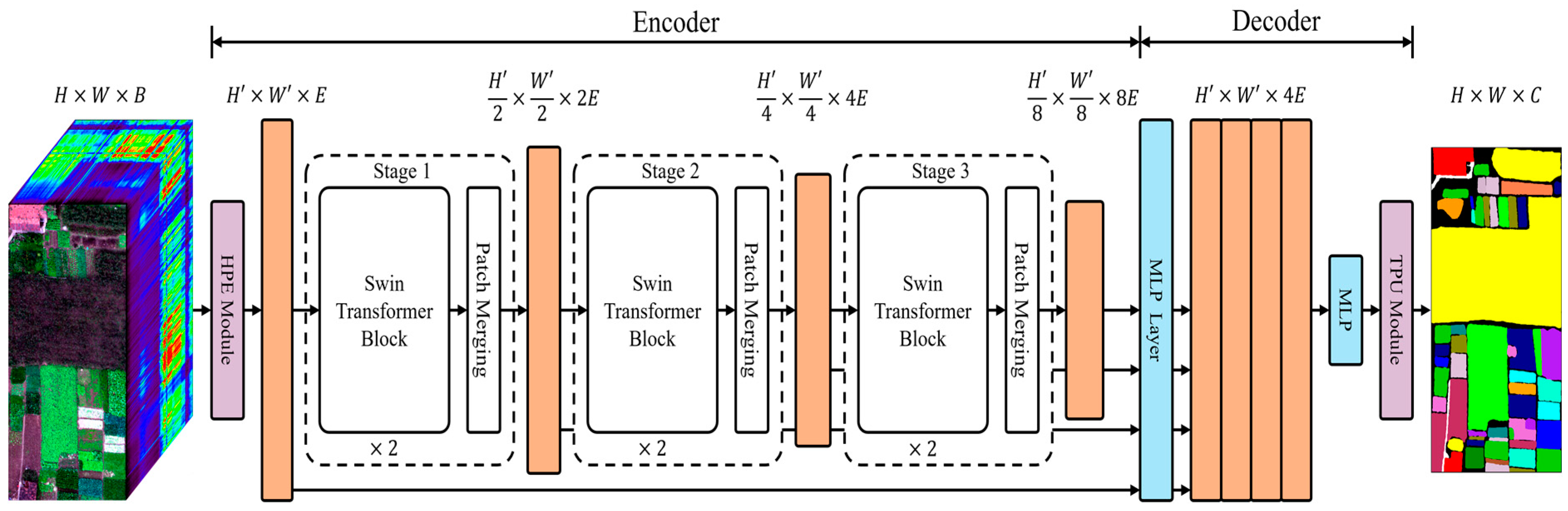
3. HyperSFormer

This section reviews knowledge of the classical transformer architecture and proposes the HyperSFormer method. The model is a complete end-to-end hyperspectral image classification model, which implements end-to-end image segmentation by learning the mapping $f*:R^{H\times W\times B}\to R^{H\times W\times C}$. As illustrated in Figure 1, the model converts hyperspectral images into embedding vectors that are suitable for the Swin Transformer architecture through the HPE module. It initially extracts both local spatial and global spectral context information from the images. The uniquely designed Swin Transformer encoder extracts feature maps of various sizes and levels, which are then fused by the decoder using the improved SegFormer. This fusion allows for thorough learning of the spatial context information within different sample ranges. The inclusion of the TPU module preserves the original image size information during decoding, which is crucial for achieving end-to-end hyperspectral image classification. Additionally, the AMLS sampling strategy addresses the issue of insufficient and imbalanced training samples in the hyperspectral image classification dataset. To ensure fast model convergence, a loss function specifically tailored for hyperspectral image classification is designed.

3.1. Swin Transformer

The transformer architecture is a deep learning architecture utterly unlike the CNN and RNN and was first used in NLP. Due to its good results in dealing with sequence-to-sequence problems (e.g., machine translation and text summary generation), researchers have stopped using the RNN, which is a one-way-only sequence processing architecture, and enabled the model to capture global information at any position in the sequence through the powerful self-attention mechanism in the transformer [28]. Beyond NLP, the computer vision field has also begun to re-evaluate the limitations of CNNs and explore the potential of the transformer architecture in improving model performance [29].

The ViT pioneered using the transformer architecture for better results in computer vision [24]. The model divides an image into blocks and encodes the position so that the image is transformed into the embedding vector that can be input into the transformer encoder while adding the cls embedding to the input to achieve the effect of image classification. The Swin Transformer proposed by Liu et al. [30] is another great success of the transformer architecture in computer vision. After re-evaluating the limitations of the ViT model, the Swin Transformer employs shifted windows and a multi-level feature map design similar to that of the CNN model, achieving better results than the CNN-based model in tasks in computer vision (image classification, object detection, semantic segmentation, etc.). Because it is more suitable for extracting sequence information features, it has attracted increasing attention in video understanding, multimodal, and other fields. The transformer architecture provides a new solution and creative thinking for computer vision-related tasks.

The success of the transformer architecture heavily relies on the self-attention module for extracting internal information from the sequence. In contrast to CNN, the transformer encoder decreases its reliance on external information by stacking and integrating multiple self-attention modules, resulting in the formation of multihead self-attention (MSA). The specific pseudocode for the MSA module is provided in Algorithm 1.

Algorithm 1 multi-head self-attention

1: Input: $\mathit{X}=(x_1,\cdots ,x_n)$: a sequence data, where $x_i$ has m length 2:      ${\mathbf{W}}_{\mathrm{q}},{\mathbf{W}}_{\mathrm{k}},{\mathbf{W}}_{\mathrm{v}}$: three transformation matrices of $m\times m$ 3:      ${\mathrm{N}}_{\mathrm{head}}$: the number of multi-head 4: Output: Z: a sequence data 5:      $\mathit{Q}=({\mathrm{q}}_1,...,{\mathrm{q}}_{\mathrm{m}})⟵{\mathit{W}}_{\mathit{q}}\mathit{X}$ 6:      $\mathit{K}=({\mathrm{k}}_1,...,{\mathrm{k}}_{\mathrm{m}})⟵{\mathit{W}}_{\mathit{k}}\mathit{X}$ 7:      $\mathit{V}=({\mathrm{v}}_1,...,{\mathrm{v}}_{\mathrm{m}})⟵{\mathit{W}}_{\mathit{v}}\mathit{X}$ 8:      $d⟵\frac{\mathrm{m}}{{\mathrm{N}}_{\mathrm{h}\mathrm{e}\mathrm{a}\mathrm{d}}}$ 9:      $\mathit{Z}⟵\mathrm{s}\mathrm{o}\mathrm{f}\mathrm{t}\mathrm{m}\mathrm{a}\mathrm{x}\left(\frac{\mathit{Q}{\mathit{K}}^{\mathit{T}}}{\sqrt{d}}\right)\mathit{V}$

10:      return $\mathit{Z}$

However, the self-attentive module only operates on the encoded vector of the image and does not preserve the location information. This module has specific restrictions on the information extraction of image data containing local information; therefore, the ViT conducts position coding to retain image position information when patch embedding. The Swin Transformer improves based on the ViT and retains position information through relative position encoding for each pixel during MSA. Additionally, the Swin Transformer adopts a patch merging module to achieve a hierarchical architecture similar to that of a CNN, thereby allowing the model to effectively handle images of varying scales. This approach involves creating a new image by selecting elements at regular intervals in the row and column directions, resulting in a reduced length and width. Subsequently, all merged images pass through a fully connected layer to alter the channel size from four times the original to twice the original dimensions. For a visual representation of this specific implementation, refer to Figure 2.

The Swin Transformer divides the input image into non-overlapping windows of a fixed size and performs MSA calculations on various windows to achieve the window MSA (W-MSA) operation to reduce the computational effort. The W-MSA makes the complexity of the model in computation linear only for the height and width of the image. The computational complexity of the W-MSA operation and MSA operation on an image with a size of $H\times W$ and number of channels $E$ is as follows:

$$\mathsf{\Omega }\left(\mathrm{M}\mathrm{S}\mathrm{A}\right)=4HW{E}^2+2(HW{)}^{2}E$$

(1)

$$\mathsf{\Omega }\left(\mathrm{W}-\mathrm{M}\mathrm{S}\mathrm{A}\right)=4HW{E}^2+2M^{2}HWE$$

(2)

Although W-MSA can reduce the computational complexity of the transformer architecture, the lack of information communication between non-overlapping windows loses the ability to extract global information using MSA. Thus, the shifted window MSA (SW-MSA) operation is introduced to realize the information between windows. As depicted in Figure 3, SW-MSA shifts the original division by half the window size in two adjacent Swin Transformer blocks to obtain the new division.

However, this operation presents an additional challenge in terms of computational complexity, as depicted in Figure 3. This change results in an increase in the utilization of the MSA module from four to nine times. To address this issue, the cyclic shift operation is employed. It concatenates the windows that would otherwise have been divided prior to conducting the SW-MSA process. By doing so, the computational complexity remains unchanged while effectively facilitating information interaction across different windows.

3.2. SegFormer

In previous research on semantic segmentation models, most of the work investigates how to design better decoders (e.g., adding more feature map fusion patterns), which leads to increasingly larger decoders for the models. With the growing utilization of the Transformer architecture in computer vision, its application of serialized feature vectors allows for a reduction in decoder architecture complexity. SegFormer presents a straightforward, efficient, and resilient semantic segmentation model. It employs an encoder based on the transformer architecture and a decoder comprising only a few MLPs. This model achieves state-of-the-art (SOTA) performance on well-established semantic segmentation datasets such as ADE20K and Cityscapes, all while considering segmentation speed. Similarly, SegFormer delivers remarkable results, showcasing improved robustness, on datasets contaminated with various forms of noise, such as Cityscapes-C.

In SegFormer, the encoder generates a sequence of feature vectors as its output. To handle feature sequences of different scales, the feature sequence is expanded into a feature map, which is only one-fourth the size of the original image, using the MLP architecture. The transformed feature maps from each level are then merged, followed by channel reduction through an MLP, resulting in segmented categories for obtaining the prediction results. The decoder architecture in SegFormer solely comprises the MLP, avoiding the introduction of complex operations such as dilated convolution or bidirectional feature pyramid network (Bi-FPN). This design choice ensures the efficiency and effectiveness of the decoder operation.

3.3. Hyper Patch Embedding and Transpose Padding Upsample Module

In the Swin Transformer, the RGB image of size $H\times W\times 3$ is transformed into tokens of size $\frac{H}{4}\times \frac{W}{4}\times 48$ through patch embedding. These tokens are then inputted into the Swin Transformer block. Specifically, the image is first divided into square patches using two-dimensional convolution, with each patch having a patch size of 4 × 4. These patches are then concatenated as individual tokens and fed into the model.

Unlike the Swin Transformer, which processes dissimilar discrete sequences as input features, hyperspectral images contain data obtained from densely sampled spectral channels across the electromagnetic spectrum. It is common for neighboring channels in hyperspectral images to exhibit similarities due to the tiny sampling intervals. The crucial aspect for accurate classification of hyperspectral images lies in capturing the most expressive features from the nearly continuous spectral information.

Therefore, the hyper patch embedding (HPE) module is added before the input Swin Transformer block in this paper. The implementation process of the entire HPE is illustrated in Figure 4. Given a hyperspectral image, as shown in the “Patch” operation of Figure 4, we initially apply a two-dimensional convolution to extract local spatial features with a patch size of $PatchSize\times PatchSize$. This process simultaneously extracts spectral features while reducing the channel dimension to the size of $EmbedDim$. To ensure the model’s generalizability across different datasets, we perform a “Pad” operation on the hyperspectral image, resulting in $H^{\prime }$ and $W^{\prime }$ and satisfying the following equation:

$$2^{3}WindowSize\mid H^{\prime },2^{3}WindowSize\mid W^{\prime }$$

(3)

Here, $WindowSize$ refers to the sliding window size designed in the Swin Transformer block, and $2^3$ is determined by the three downsampling operations performed by the model. Finally, the padded hyperspectral image is passed through a simple multilayer perceptron (MLP) to capture the global spatial context at the initial stage of the model. Subsequently, the image is unfolded and normalized before being fed as input to the encoder.

Given all of the features in a hyperspectral image, the local spatial features are extracted according to a predefined $PatchSize$, and each patch is considered a token. The number of channels of spectral features is reduced from the original number of channels to the $EmbeddedDim$ to extract spectral features. Furthermore, to ensure model adaptability to arbitrary datasets, the height and width of the extracted hyperspectral image must be padded to satisfy certain conditions.

Finally, the filled hyperspectral image is completed once with MLP operation, and the images in each extracted spectral feature are expanded and normalized as the encoder input. The details are provided in Figure 4.

After the lightweight encoder in SegFormer, bilinear interpolation restores the fused feature map of the decoder to its original size. This method can significantly improve the efficiency of model segmentation for the semantic segmentation task of RGB images, but it is not applicable to the hyperspectral image classification task. In hyperspectral image classification, because the images are taken using remote sensing techniques, one pixel often represents a large piece of the actual area, and the prediction results must be accurate to the pixel level.

In this paper, we designed the transpose padding upsample (TPU) module based on the output of the decoder in SegFormer. The fused feature map can be restored to the original size of the image using the TPU module. Figure 5 illustrates the details of the TPU module. In this module, we first extract features between pixels surrounding the original pixels in different channels through the “Transpose” operation. Specifically, the feature maps are enlarged by $PatchSize$ times, and the channel dimension is halved, which can be achieved using two-dimensional convolution. Subsequently, the enlarged image is cropped back to its original size using the “Cut” operation. Finally, a simple MLP is employed to map the channel dimension to the number of classes, $C$, enabling end-to-end prediction.

3.4. Adaptive Min Log Sampling Strategy and Loss Function

The problem of insufficient and imbalanced training samples in hyperspectral image classification has been a critical problem to be solved in this field. The number of labeled samples in each category varies widely. When the traditional sampling strategy is used, where a fixed number of samples are randomly selected from all samples in each category as training samples, it leads to a significant limitation in the average and overall model accuracy due to the imbalance between the number of training samples. To make the model learn more discriminative features and enhance the robustness of model classification, the sampling strategy of adaptive min log sampling (AMLS) is used, formally described in Algorithm 2.

Algorithm 2 adaptive min log sampling

$1:\mathbf{Input}:\mathit{A}={\left\{a_i\right\}}_{i=1}^{H\times W}$: a set of labels for training $2: \mathit{N}$: the number of class where not included negative classes $3: s$: the Sampling magnification $4: \alpha$: mini-batch per class $5:\mathbf{Output}:\mathit{M}\mathit{T}$: a list of sets of stratified labels $6: T\leftarrow [ ]$: an empty list 7: for k = 0 to N do $8: Inde{x}_k\leftarrow \{i\mid a_i=k,a_i\in A\}$ $9: nu{m}_k\leftarrow$ the number of $Inde{x}_k$ 10: end for $11:nu{m}_{min}\leftarrow$ the minimum of $nu{m}_k$ 12: for k = 0 to N do $13: RS\leftarrow {\mathrm{l}\mathrm{o}\mathrm{g}}_2\left(\frac{nu{m}_k}{nu{m}_{min}}\right)+1$ $14: Sampl{e}_k\leftarrow RS\ast nu{m}_{min}\ast s$

$15: TrainInde{x}_k\leftarrow$ Randomly sample $Sampl{e}_k$ samples from $Inde{x}_k$ 16: end for 17: repeat 18: for k = 0 to N do $19: T_k\leftarrow$$\mathrm{Randomly}\mathrm{sample}TrainInde{x}_k$ $\mathrm{samples}\mathrm{from}\lceil \frac{Sampl{e}_k}{\alpha }\rceil$ $20: MT.push\left(T_k\right)$ 21: end for

In the AMLS strategy, the training samples are taken from the whole image rather than the divided image blocks. Discrete training sample sequences are extracted from the entire hyperspectral image according to the above algorithm, and other samples that are not selected as training samples are used as testing samples. The training samples are randomly selected from the training sample sequence during training to reduce the training time and improve the model robustness. Most current models only consider the positive samples in the image during training. However, they do not consider the unlabeled negative samples in the image, leading to the possibility of misclassifying some negative samples as positive samples during classification and making the final generated prediction images less accurate. In the strategy proposed in this paper, negative samples are uniformly labeled as Class 0. Before sampling, one must iterate over the sample count of each class and store the indices of each class’s samples in the corresponding ${Index}_k$ list. Then, based on the class with the minimum sample count and the sampling factor $s$, the number of training samples for each sample is determined as ${Sample}_k$. Using the training sample count for each sample, training samples are randomly selected from the ${Index}_k$ list of each class to obtain the training sample sequence $TrainIndex$ for the hyperspectral image. In each subsequent epoch of training, samples $T_k$ are randomly selected from $TrainIndex$ for training, based on ${Sample}_k$ and the hyperparameter $\alpha$. Here, the aforementioned sampling factor $s$ is determined by the class with the minimum sample count and the dataset. By using the formula, it can be observed that when calculating the training sample count for the class with the minimum sample count, $RS$ is equal to 1, resulting in $Sample\_k$ being ${num}_{min}\ast s$. By referring to relevant literature on the dataset, the commonly used sample count for the class with the minimum sample count during training is obtained, and the sampling factor $s$ is determined accordingly. The hyperparameter $\alpha$ mentioned above is determined per training epoch. In this study, the hyperparameter $\alpha$ is set to 0.2.

Similarly, in hyperspectral image classification, the selected training sample size is logarithmically calculated to dilute the gap between the original sample sizes. However, due to the massive gap between the number of original samples in some datasets, the problem of slow convergence caused by the gap between the number of samples in different categories must still be considered during training. A loss function more suitable for hyperspectral image classification is designed in this paper to address the above problems. The specific formula is as follows:

$$\mathcal{L}=\frac{1}{N}{\sum }_{i=0}^N\beta {\mathcal{L}}_{Dice}^k+(1-\beta ){\mathcal{L}}_{Focal}^k$$

(4)

In hyperspectral image classification, the architecture between pixel points is strongly regionally correlated, and the same categories tend to be clustered together, with clear demarcations between categories. Thus, the pixel loss and gradient update are related to the predicted and actual values of that point and other points around that point. Milletari et al. [31] proposed dice loss to calculate this strong correlation loss, and dice loss is very effective in balancing positive and negative samples to identify the foreground and background regions of an image effectively. The specific formula is as follows:

$${\mathcal{L}}_{Dice}^k=1-\frac{2p_k{t}_k}{\left(p_k+t_k\right)}$$

(5)

where $p_k\in [0,1]$ is the probability that all training samples predict category $k$, $t_k\in \{0,1\}$ is the actual value of all training samples (i.e., those not for category $k$ have a value of $0$ and those for category $k$ have a value of $1$).

An improved binary cross entropy (BCE) loss called focal loss [32] was used for the sample gap between classes of hyperspectral images. By adding sample size weights before the BCE loss, the model reduces the weight of easily classifiable samples and focuses more on the difficult-to-classify samples during training.

Specifically, we define $E_k$ as the weight for balancing difficult samples, calculated as follows:

$$E_k^i=\left\{\begin{array}{c}{p}_k^i, t_k^i=1\\ 1-p_k^i, \mathrm{otherwise}\end{array}\right.$$

(6)

where $i$ represents the point in the training sample when the actual value of the point is category $k$ and $E_k^i$ takes the value of the predicted probability of the point; otherwise, it is $1$ minus the predicted probability of the point. In general, the formula can be written as follows when calculating $E_k$ for that category:

$$E_k=p_k{t}_k+(1-p_k)(1-t_k)$$

(7)

Therefore, the specific formula of focal loss is given as follows:

$${\mathcal{L}}_{Focal}^k=-(1-E_k{)}^{\gamma }\mathrm{l}\mathrm{o}\mathrm{g}(E_k)$$

(8)

where $\gamma >0$ is an adjustable parameter to adjust the ratio of the difficult and easy weights, and in this paper, $\gamma$ is set to 2. In the formula for the total loss function, $\beta \in \left(0,1\right)$ is used to adjust the weights between the two loss functions, and $\beta$ is set to 0.7.

With the above loss function, the AMLS strategy ensures a balanced distribution of categories in the training samples while obtaining stable and diverse gradients by sampling small batches. The designed loss function can consider both positive and negative samples while distinguishing between difficult and easy samples, ensuring the stability and randomness of the gradient and accelerating the training speed.

4. Results

The HyperSFormer method is compared with current hyperspectral image classification methods, including FPGA, SSDGL, and SegFormer, to quantitatively and qualitatively analyze its performance and is extensively validated on three datasets. Different datasets were used to verify the effectiveness of HyperSFormer in the presence of imbalanced sample data, complex negative samples, and mixed sample categories. All experiments were performed on a PyTorch library on a machine with a 3080 Ti graphics card.

4.1. Experimental Settings

4.1.1. Model Parameters

The HyperSFormer method is based on encoding and decoding. There are differences in data sizes in different datasets, and to ensure the data meet the model requirements as closely as possible, the HPE module designed in this paper ensures the adaptive input of images and extracts spectral features, keeping the spectral features in the $EmbedDim$ size. In this paper, the selected $PatchSize$ is 2, and $EmbedDim$ is 64. The described experiments were conducted under the condition that the random number seeds were fixed to ensure the reliability of the experiments.

4.1.2. Optimized Parameters

The optimizer plays a crucial role in training deep learning models, and an optimizer that is suitable for the model ensures fast model convergence. The HyperSFormer model performed 1200 epochs for each dataset and used the AdamW optimization algorithm with an initial learning rate of 1 × 10⁻³ and a weight decay of 1 × 10⁻⁵. The learning rate decay method used cosine annealing [33] on the learning rate iterations, which decay in each decay cycle with the formula:

$${\eta }_t={\eta }_{min}+\frac{1}{2}({\eta }_{max}-{\eta }_{min})(1+\mathrm{c}\mathrm{o}\mathrm{s}(\frac{T_{cur}}{T_i}\pi \left)\right)$$

(9)

where ${\eta }_{max}$ and ${\eta }_{min}$ denote the maximum and minimum values of the set learning rate, respectively, $T_{cur}$ indicates the number of trained rounds in the current cycle, $T_i$ represents the total number of training rounds in the current cycle, and $T_i$ is calculated as follows:

$$T_i=T{T}_{mult}^{i-1}$$

(10)

In this paper, $T$ is set at 50, which is the unit of the first decay cycle, and $T_{mult}$ is set to 23, which represents the incremental multiplier of each cycle.

4.1.3. Metrics

To evaluate the performance gap between HyperSFormer and other methods, four commonly used hyperspectral image classification metrics are used to measure the accuracy of each class, the overall accuracy (OA), the average accuracy (AA), and the kappa coefficient (Kappa). Besides the common indicators, the standard metric mean intersection over union (mIoU) in image segmentation is also introduced as the overall image evaluation index, and the formula is:

$$mIoU=\frac{1}{C}{\sum }_{i=0}^C\frac{p_{ii}}{\sum _{j=0}^C{p}_{ij}+\sum _{j=0}^C{p}_{ji}-p_{ii}}$$

(11)

where $C$ represents the total number of categories in the dataset and $p_{ij}$ indicates the total number of samples whose actual value is class $i$ predicted to be class $j$ at the time of prediction.

In addition, this paper introduces model parameters (Params) and floating point operations per second (FLOPs) as comparative metrics to assess the performance of various models.

4.2. Experiment 1: Indian Pines Dataset

The Indian Pines dataset was collected using the airborne visible infrared imaging spectrometer (AVIRIS) sensor in northwestern Indiana, USA. This dataset is the earliest hyperspectral image classification dataset and contains 145 × 145 pixels with 220 spectral bands with a wavelength range covering 400 to 2500 nm, containing 16 agricultural crop types. Figure 6 illustrates the three-band false-color composite and ground-truth map of this dataset. In this paper, to test the ability of the model to filter the bands, the model inputs were selected for all 220 bands without noise removal.

Table 1. Number of samples and classification results for the Indian Pines dataset.

No.	Class	Sample		Method Accuracy
		Total	Train	FPGA	SSDGL	SegFormer	HyperSFormer
0	Background	10776	67	0.0	77.8	69.4	97.1
1	Alfalfa	46	14	100.0	100.0	100.0	100.0
2	Corn—no till	1428	47	95.0	99.0	86.8	99.4
3	Corn—min till	830	42	94.8	99.5	93.4	99.5
4	Corn	237	30	100.0	100.0	99.2	100.0
5	Grass—pasture	483	37	99.2	100.0	91.5	99.8
6	Grass—trees	730	41	99.2	100.0	97.4	98.8
7	Grass—pasture-mowed	28	9	100.0	100.0	100.0	100.0
8	Hay—windrowed	478	37	100.0	100.0	90.2	100.0
9	Oats	20	6	100.0	100.0	100.0	100.0
10	Soybean—no till	972	44	99.2	99.3	83.5	99.6
11	Soybean—min till	2455	52	95.5	98.7	93.7	99.8
12	Soybean—clean	593	39	99.3	99.5	92.6	99.3
13	Wheat	205	29	100.0	100.0	100.0	100.0
14	Woods	1265	46	99.4	99.3	92.1	99.7
15	Buildings–Grass–Trees–Drives	386	35	100.0	100.0	98.4	99.7
16	Stone–Steel Towers	93	21	100.0	100.0	98.9	100.0
Metrics	Overall accuracy (%)			47.5	39.9	80.4	98.4
	Average accuracy (%)			93.0	94.0	93.4	99.6
	Kappa			0.447	0.371	0.746	0.977
	mIoU (%)			42.5	41.2	61.3	98.0
	Params (M)			2.67	2.31	4.06	2.93
	FLOPs (G)			15.48	29.05	1.06	3.16

The bold represents the best value of the metric among all validated models.

lists the number of training samples for each category obtained by the Indian Pines dataset through the AMLS strategy, where the sampling factor $s$ in AMLS is taken as one-third.

The accuracy and evaluation metrics for all methods for all categories are presented in Table 1, and the best accuracy for each row is highlighted in bold to validate the HyperSFormer in more detail. As listed in Table 1, the methods based on semantic segmentation have high accuracy for all single-class targets, and the OA is above 90%, primarily attributed to HyperSFormer for global spectral contextual information feature extraction. Compared with FPGA and SSDGL, HyperSFormer achieves about a 3% improvement in AA. After adding negative samples for training, the classification accuracy of the model did not decrease significantly, and there was a significant improvement in the classification accuracy for negative classes. The values of OA and mIoU were improved, leading to a higher OA of the model. In addition, the AMLS strategy plays a vital role in the problem of sample imbalance, with dice loss allowing the model to balance more positive and negative samples during training and focal loss reducing the weight of easily classified samples, allowing the model to focus more on the difficult-to-classify samples during training. Table 1 reveals that, under the joint action of the AMLS strategy and loss function, the classification accuracy of corn—no till, partial—min till, and other hard classification categories is higher than that for the FPGA and SSDGL. Thus, the proposed method achieves promising results on insufficient and imbalanced datasets. Simultaneously, during the evaluation of model efficacy, it can be found by comparing Params and FLOPs that the method proposed herein substantially enhances computational velocity in comparison to FPGA and SSDGL, concomitantly ameliorating model precision with merely a marginal escalation in parameter quantity.

Figure 7 depicts the classification results using FPGA, SSDGL, SegFormer, and HyperSFormer. In the hyperspectral image classification method based on semantic segmentation, it is evident that each category has firm category boundaries whether negative samples are added or not. This outcome is because the method based on semantic segmentation can fully use the global spatial context information to extract more discriminative spatial features during training. Comparing Figure 7A–D, the model classification effect has better visual performance because adding negative samples to the training enables the model to extract the features of negative samples to distinguish the difference between positive and negative samples. In addition, there is more consideration for the recognition of different samples. Compared with SegFormer, the classification results for HyperSFormer are more accurate at the edges of adjacent categories because the TPU module removes the limitation of bilinear interpolation in the SegFormer model to restore the original image size. Moreover, it considers the center and edges of the same sample region after feature map fusion.

4.3. Experiment 2: WHU-Hi-HanChuan Dataset

This paper conducts experiments on the WHU-Hi-HanChuan dataset to further evaluate the effectiveness of HyperSFormer in the case of negative sample complexity in particular. The WHU-Hi dataset is a benchmark dataset built and published by Zhong et al. [34] for training and evaluating agricultural crop classification tasks. The WHU-Hi-HanChuan dataset consists of seven agricultural crop types collected on 17 June 2016, via the Leica Aibot X6 uncrewed aerial vehicle V1, which was flown and photographed under clear and cloudless weather conditions at an altitude of 250 m with a spatial resolution of 10.9 cm. The pixel size of the dataset is 1217 × 303, and the band range is from 400 to 1000 nm, with 274 bands. The images were taken in the afternoon; therefore, many shadowed parts in the collected hyperspectral images added difficulty to the agricultural crop classification. The number of training samples per category in the WHU-Hi-HanChuan dataset is obtained using an AMLS strategy with a sampling factor $s$ of one-tenth. Figure 8 presents the three-band false-color composite and ground-truth map of this dataset.

To quantitatively evaluate the performance of the above methods on this dataset, Figure 9 illustrates the OA, AA, kappa coefficients, and mIoU. Because the spatial resolution of this dataset is very high, spatial context information is vital for hyperspectral images to distinguish difficult-to-classify classes. The HyperSFormer model introduces the HPE module to establish interdependencies based on continuous spectral sequence information and global spatial context information, achieving the best accuracy in most categories. The accuracy of using HyperSFormer for categories other than the shaded negative samples is generally higher than 95% and more stable than either FPGA and SSDGL. This result is primarily attributed to the AMLS strategy, which sets different training samples for various sample sizes and appropriately increases the number of training samples for hard training samples, effectively improving model performance. Moreover, HyperSFormer has higher accuracy for the OA, AA, kappa coefficient, and mIoU, where OA is higher than the FPGA without using shaded negative samples by more than 5% and higher than SSDGL without using shaded negative samples by about 1% in all metrics.

Figure 10 illustrates the classification results obtained using FPGA, SSDGL, SegFormer, and HyperSFormer. The classification results of the FPGA exhibit color mixing in the boundary region, implying uncertainty in the model’s classification without the inclusion of negative samples. The presence of shadow coverage in the dataset poses a significant challenge in identifying the black-shaded parts. These shadow locations are scattered among different classes, making it difficult to distinguish them based on spatial context information alone. Therefore, effective spectral features must be extracted. The classification results show that the shaded parts (negative samples) differ significantly in the level of detail across the various methods. However, HyperSFormer is capable of accurately identifying all shaded parts and distinguishing the negative samples. Additionally, HyperSFormer outperforms other methods in classifying difficult samples. This performance is attributed to the fusion loss function used during training, which reduces the weight assigned to easily classifiable samples and prioritizes challenging-to-classify samples.

4.4. Experiment 3: WHU-Hi-HongHu Dataset

Although the proposed method, HyperSFormer, based on the transformer and semantic segmentation, achieves promising results on the Indian Pines and WHU-Hi-HanChuan datasets, the total number of classes in these two datasets is only 16. We selected the WHU-Hi-HongHu dataset for Experiment 3, which comprises 17 varieties of three major crop types: cotton, oilseed rape, and kale. The acquired images were obtained on 20 November 2017, with DJI Matrice 600 Pro, using the device in cloudy weather at an altitude of 100 m above the ground and with a spatial resolution of 4.3 cm. The size of the captured hyperspectral image is 940 × 475. The number of bands is 270, and the band range is between 400 and 1000 nm. The dataset has 22 categories that provide a good response to the classification ability of the model in the presence of mixed sample categories. Figure 11 illustrates the three-band false-color composite and ground-truth map of this dataset. The number of training samples per category in the WHU-Hi-HongHu dataset is obtained using an AMLS strategy with a sampling factor $s$ of one-tenth.

Figure 12 depicts the classification results using FPGA, SSDGL, SegFormer, and HyperSFormer, revealing that HyperSFormer has superior classification performance compared with other popular methods based on semantic segmentation. Figure 13 further presents the classification effects due to the TPU module. In addition, HyperSFormer can provide a good detailed representation, where the sample categories are more mixed and the boundaries of each category are the same. Further, HyperSFormer benefits from the increased global spatial context and spectral information. The SW-MSA module uses the global spatial context embedding vector to reweight the feature maps and model the interdependencies between feature maps, facilitating the classification of the hyperspectral images with redundant spectral information. Compared with SegFormer, HyperSFormer solves the problem that the results of methods based on the transformer and semantic segmentation are insufficiently accurate. Additionally, the transformer architecture can make an essential breakthrough in the multiclassification of hyperspectral images.

5. Discussion

We conducted extensive analytical experiments on each parameter setting to understand the effectiveness of the HyperSFormer model parameter settings better. All analytical experiments were performed on the Indian Pines dataset with low spatial resolution and unbalanced sample data.

5.1. Discussion of Different Models

Table 2. Model evaluation results with different models in the Indian Pines dataset.

	HyperSformer	SegFormer	DeepLabv3 Plus	U-Net	PSPNet
OA	98.4	80.4	93.2	96.1	92.0
AA	99.6	93.4	97.9	99.1	97.3
Kappa	0.977	0.746	0.907	0.946	0.891
mIoU	98.0	61.3	91.4	95.1	86.4
Params (M)	2.93	4.06	7.67	5.84	6.74
FLOPs (G)	3.16	1.06	7.32	5.15	3.95

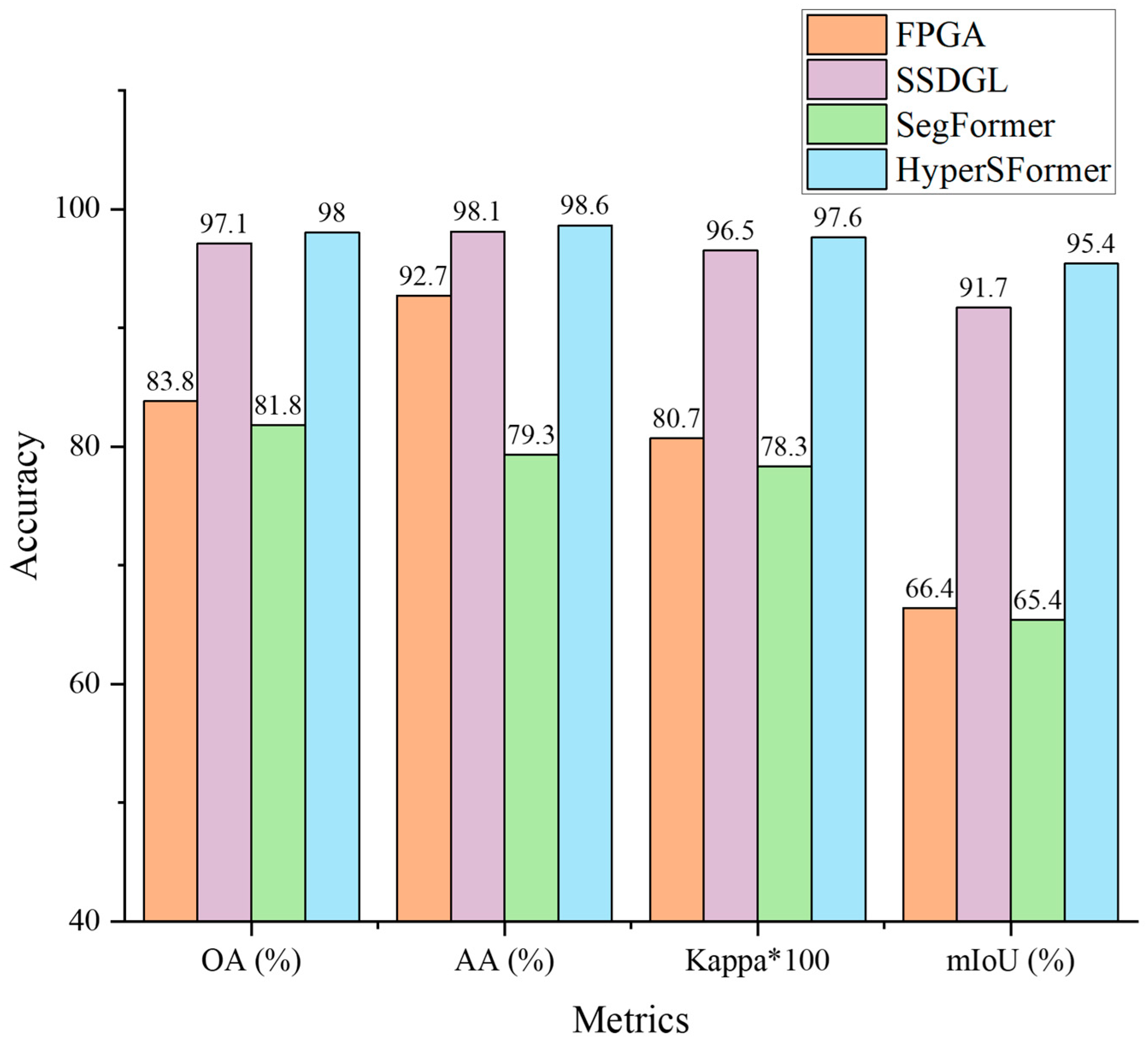
The bold represents the best value of the metric among all validated models.

displays a comparative analysis of our model against several semantic segmentation models. Evidently, the computational complexity associated with transformer-based architectures is predominantly lower in comparison to their CNN-based counterparts. HyperSFormer manages to maintain reduced computational complexity while simultaneously minimizing the number of parameters involved.

5.2. Discussion of the HPE Parameters

Table 3. Model evaluation results with $PatchSize$ and $EmbeddedDim$ in the Indian Pines dataset.

		Baseline	Evaluation 1				Evaluation 2			NO_HPE
Model param	Patch Size	2	1	3	4	5	2	2	2	/
	Embedded Dim	64	64	64	64	64	32	80	96	/
Metric	OA	98.4	97.7	97.4	98.0	95.1	96.3	96.5	97.1	98.0
	AA	99.6	99.1	98.9	99.4	98.5	98.0	98.6	99.0	90.2
	Kappa	0.977	0.968	0.963	0.971	0.932	0.949	0.952	0.960	0.971
	mIoU	98.0	96.7	96.7	96.8	92.1	93.7	95.6	96.3	89.7

The bold represents the best value of the metric among all validated models.

delineates the classification performance of the model using various combinations of hyperparameters. The benchmark method encompasses the model parameter configurations utilized in the preceding section. In contrast to the model devoid of the HPE module, the model incorporating the HPE module exhibits superior classification capacity for both positive and negative instances, culminating in a higher AA compared to its counterpart without the HPE module.

The hyperparameter $PatchSize$ is the unit for chunking images in the HPE module. Table 3 reveals that the model works best when the $PatchSize$ is set to 2 because the model initially extracts the neighboring spatial features in the hyperspectral images in the HPE. If the $PatchSize$ is too large, the model focuses too much on the surrounding features instead of those that should be extracted, degrading classification accuracy. If the $PatchSize$ is set to 1, the model only learns its own channel information and not the neighboring spatial features, which also decreases classification accuracy.

The hyperparameter $EmbeddedDim$ is introduced in the HPE module to determine the number of compressed channels in the spectral space and is also the basic unit of vector dimensionality in the Swin Transformer block. Table 3 indicates that when $EmbeddedDim$ is lower or higher, the model does not perform as well as when it is set to 64 because when set low, the limited number of channels is too small to learn all spatial and spectral features. When $EmbeddedDim$ is set high, the model becomes too redundant, making the model too scattered in feature learning, focusing on features that should not be focused on, and causing the training time to increase significantly.

5.3. Discussion of the Loss

Table 4. Model evaluation results for training with loss functions in the Indian Pines dataset.

	Cross-Entropy Loss	$\mathit{\beta }$$\mathbf{Dice}\mathbf{Loss}+(1-\mathit{\beta })$ Focal Loss
$\beta$	/	1	0.7	0.5	0.3	0
OA	72.4	97.8	98.4	96.7	95.1	74.7
AA	88.9	84.9	99.6	98.8	98.3	90.8
Kappa	0.659	0.968	0.977	0.954	0.932	0.685
mIoU	0.528	84.4	98.0	95.5	89.6	59.3

presents the effect of training HyperSFormer using various loss functions to demonstrate the reasonableness of the loss function settings. The hyperparameter $\beta$ is used to set the ratio between the dice loss and focal loss. Table 4 reveals that training the model with cross-entropy loss and focal loss results in higher AA metrics than OA metrics in the final results of the model, indicating that the two loss functions are good at classifying each class. The model focuses on both difficult- and easy-to-classify samples but not enough for the overall classification effect, and it cannot effectively balance the gap between positive and negative samples. Moreover, the model is better trained using the focal loss than cross-entropy loss, which is consistent with the setting, where it is a cross-entropy loss improvement algorithm. In addition, Table 4 reveals that the OA with only dice loss is much higher than AA because the dice loss focuses on the background information in the sample in addition to the foreground information and determines the most discriminative features from the positive and negative samples.

In the fused loss function of dice loss and focal loss proposed in this paper, the overall classification performance using the fused loss function is better than that of the single loss function. Adding focal loss compensates for the lack of discriminative power of using the dice loss for difficult-to-classify samples. The value of $\beta$ does not have a substantial influence on the classification performance but still plays a key role, and the model is best trained when $\beta$ is 0.7.

5.4. Discussion of the Sampling Strategy

Table 5. The validation results of the HyperSFormer model using different sampling strategies were evaluated on the Indian Pines dataset.

	Class	Total	HperSFormer + GS2	HperSFormer + H-B	HperSFormer + AMLS
Sample Num	0	10,776	0	539	67
	1	46	46	5	14
	2	1428	100	72	47
	3	830	100	42	42
	4	237	100	12	30
	5	483	100	25	37
	6	730	100	37	41
	7	28	28	5	9
	8	478	100	24	37
	9	20	20	5	6
	10	972	100	49	44
	11	2455	100	123	52
	12	593	100	30	39
	13	205	100	11	29
	14	1265	100	64	46
	15	386	100	20	35
	16	93	93	5	21
Metric	total	21,025	1387	1068	596
	OA		48.6	97.1	98.4
	AA		94.0	95.1	99.6
	Kappa		0.469	0.959	0.977
	mIoU		0.860	0.892	0.980
	FWIoU		0.464	0.944	0.968

presents the comparison of sample counts and validation results using the HyperSFormer architecture combined with different sampling strategies. Among them, global stochastic stratified (GS²) is the sampling strategy used in FPGA, where it simply selects 100 samples for each class for training. If there are fewer than 100 samples, all samples of that class are used for training. The hierarchically balanced (H-B) sampling strategy is used in SSDGL, where it randomly selects 5% of the sample count for each class as training samples. For classes with fewer than five samples after computation, five samples are randomly selected for training. From the data in Table 5, it can be observed that the AMLS sampling strategy selects significantly fewer training samples compared to GS² and H-B. In terms of the distribution of training samples, GS² does not consider the imbalance between different classes, while H-B only selects training samples based on the sample count of each class. This can result in inconsistent convergence speeds and larger loss weights for certain classes due to the imbalance in training samples. AMLS takes both factors into consideration by not only selecting training samples based on sample counts but also balancing the sample disparities between different classes using the class with the minimum sample count as the reference. Experimental results demonstrate that the AMLS sampling strategy achieves higher mIoU with fewer training samples.

5.5. Discussion of the HyperSFormer

The HyperSFormer proposed in this study demonstrates the effective utilization of hyperspectral images for end-to-end crop classification. This model, based on the transformer, fully incorporates both global and local spatial context as well as spectral information. The AMLS sampling strategy and fusion loss function are designed to ensure the consideration of positive and negative samples, as well as difficult and easy samples.

Although the learning-rate decay method of cosine annealing is employed in this approach, the model training still suffers from instability, and the convergence rate is marginally slower than that of the CNN-based method. Additionally, the model parameters are not yet generalized across datasets in terms of their application. To address these limitations, a future investigation will focus on developing a generalized hyperspectral image classification method, enabling the reuse of model parameters across datasets. Furthermore, training strategies will be explored to enhance the speed of model convergence.

6. Conclusions

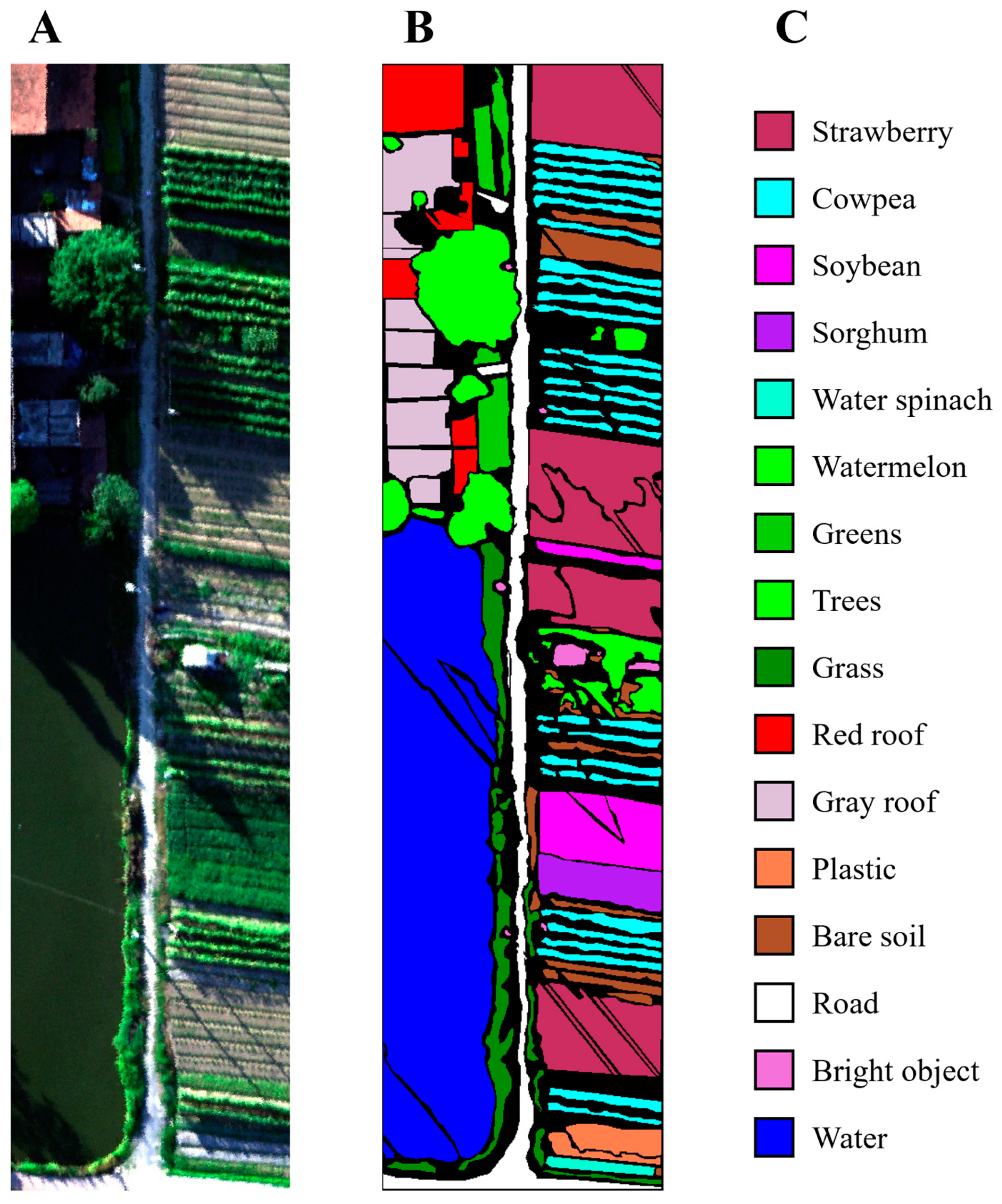
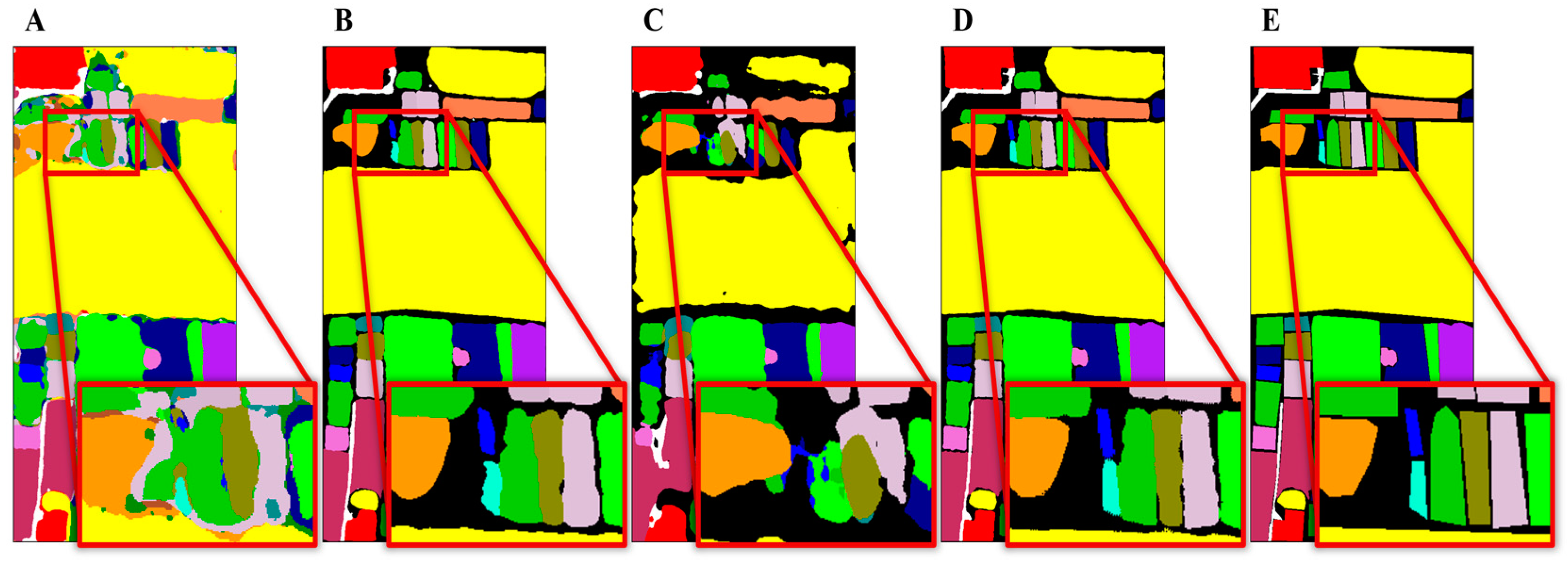
The present study introduces HyperSFormer, a crop classification method utilizing the Transformer and semantic segmentation in hyperspectral image analysis. In HyperSFormer, we replace the encoder of SegFormer with an enhanced Swin Transformer while preserving the SegFormer decoder. The entire model is characterized by a streamlined and unified transformer structure. Additionally, an HPE module and TPU module are incorporated into the model to enhance its capacity to capture global spatial context and spectral information. To address the issues of inadequate and imbalanced samples in hyperspectral image classification, we devise the AMLS strategy and a loss function that combines dice loss and focal loss, facilitating model training. Experimental findings demonstrate that HyperSFormer outperforms existing methods in terms of hyperspectral image classification, particularly when dealing with complex negative samples and mixed sample classes. Ablation experiments confirm the soundness of the model parameter design, showing that the selected parameters lead to optimal performance. Notably, the fusion loss in the designed loss function contributes significantly to the improvement. The proposed method, compared to CNN-based approaches, aligns better with the characteristics of hyperspectral images, enabling accurate hyperspectral image classification and widening the application prospects of hyperspectral image analysis in agricultural production.