Article

Super-Resolution Reconstruction of Remote Sensing Data Based on Multiple Satellite Sources for Forest Fire Smoke Segmentation

1
School of Technology, Beijing Forestry University, Beijing 100083, China
2
State Key Laboratory of Efficient Production of Forest Resources, Beijing Forestry University, Beijing 100083, China
3
School of Ecology and Nature Conservation, Beijing Forestry University, Beijing 100083, China
4
Ontario Ministry of Northern Development, Mines, Natural Resources and Forestry, Sault St. Marie, ON 279541, Canada
*
Author to whom correspondence should be addressed.
These authors contributed equally to this work.
Remote Sens. 2023, 15(17), 4180; https://doi.org/10.3390/rs15174180
Submission received: 16 May 2023 / Revised: 13 August 2023 / Accepted: 23 August 2023 / Published: 25 August 2023
(This article belongs to the Section Environmental Remote Sensing)

Abstract

:
Forest fires are one of the most devastating natural disasters, and technologies based on remote sensing satellite data for fire prevention and control have developed rapidly in recent years. Early forest fire smoke in remote sensing images, on the other hand, is thin and tiny in area, making it difficult to detect. Satellites with high spatial resolution sensors can collect high-resolution photographs of smoke, however the impact of the satellite’s repeat access time to the same area means that forest fire smoke cannot be detected in time. Because of their low spatial resolution, photos taken by satellites with shorter return durations cannot capture small regions of smoke. This paper presents an early smoke detection method for forest fires that combines a super-resolution reconstruction network and a smoke segmentation network to address these issues. First, a high-resolution remote sensing multispectral picture dataset of forest fire smoke was created, which included diverse years, seasons, areas, and land coverings. The rebuilt high-resolution images were then obtained using a super-resolution reconstruction network. To eliminate data redundancy and enhance recognition accuracy, it was determined experimentally that the M11 band (2225–2275 nm) is more sensitive to perform smoke segmentation in VIIRS images. Furthermore, it has been demonstrated experimentally that improving the accuracy of reconstructed images is more effective than improving perceptual quality for smoke recognition. The final results of the super-resolution image segmentation experiment conducted in this paper show that the smoke segmentation results have a similarity coefficient of 0.742 to the segmentation results obtained using high-resolution satellite images, indicating that our method can effectively segment smoke pixels in low-resolution remote sensing images and provide early warning of forest fires.

Graphical Abstract

1. Introduction

According to statistics, forests account for 75% of the total primary production of the Earth’s biosphere and 80% of the Earth’s plant biomass [1], with multiple economic, ecological and social benefits, and are an essential ecological support system for human life [2]. However, forests are highly vulnerable to natural disasters, such as forest fires, pests, weeds and rodents, frost damage, and wind damage, among which forest fires cause the most severe damage [3]. A forest fire is a sudden, destructive, and difficult-to-control natural disaster that can cause significant damage to humans and ecosystems [4,5,6,7].
Because smoke develops in the early phases of forest fires, identifying forest fire smoke quickly is crucial for effective forest fire control [8]. Furthermore, following a fire, smoke spreads swiftly over broad distances, and smoke particles are suspended in the air as condensation nuclei and transported by the wind, affecting air quality, climate change, forest health, water quality, and other factors [9]. Also, according to a comparison of smoke detected by satellites and visibility recorded by meteorological observers, smoke aerosols alter near-ground visibility, which has a significant impact on forest fire prevention and control [10,11]. When absorbed over time, diffuse smoke species comprise aerosols with relatively small particle sizes, which can easily lead to diseases affecting human health impacts such as respiratory infections, asthma, lung cancer, and cardiovascular ailments [12]. Consequently, the detection of small areas of early forest fire smoke, large areas of smoke from spreading fires, smoke that is intentionally ignited in an area to control the spread of forest fires, or smoke that drifts to other non-burning areas is necessary for a variety of practical applications, such as fire point detection [13], climate change modeling [14] and environmental monitoring [15]. To completely comprehend the effects of forest fire smoke, there is an urgent need for accurate, near-real-time detection of forest fire smoke.
Among different forest-fire monitoring methods, a remote sensing satellite can provide large-area, global observations with rich spatial, temporal, and spectral information [16]. Most remote sensing monitoring of forest fires utilizes the on-board sensors of low to medium spatial resolution satellites (>250 m) [17], Moderate Resolution Imaging Spectroradiometer (MODIS) [18], and Visible Infrared Imaging Radiometer Suite (VIIRS) [19]. These satellite data have a high temporal resolution (e.g., VIIRS and MODIS revisit for the same location were 24 and 12 h, respectively.), and a poor spatial resolution, thus small-area smoke of early forest fire tend to be missed based on remote sensing data with poor spatial resolution. Furthermore, high spatial resolution satellites, such as Landsat-8 with a resolution of 30 m [16] and Sentinel-2 (S2) with resolutions of 10 m, 20 m and 60 m [20], are limited by their operational orbits and cannot continuously visit the same location (revisit times of 17 and 25 days for Landsat-8 and Sentinel 2, respectively), resulting in that forest fire cannot be detected in time. In various remote sensing surveillance tasks, no combination of high spatial resolution and high temporal resolution of remote sensing data brings about a lot of severe limitations.
In order to solve the above-mentioned problems, the Super-Resolution Reconstruction (SRR) methods, which convert Low-Resolution (LR) images into High-Resolution (HR) images, have been put forward. The SR of remote sensing images can be divided into two types: single image super resolution (Single Image Super-Resolution, SISR) reconstruction and multi-image super resolution (Multi-image Super-Resolution, MISR) reconstruction. SISR can effectively enhance the spatial resolution of an image without additional information, which is more common in practical applications [21]. SISR algorithms can be classified into interpolation-based, reconstruction-based, and learning-based reconstruction. Interpolation-based reconstruction employs the source image’s element values to estimate high-resolution element values. This method is computationally simple and fast and works better with smooth images, but it is difficult to reconstruct high-frequency information and is readily influenced by high-frequency noise [22]. The reconstruction-based strategy uses a priori information to match output to input. This technique is better at enhancing edge information and suppressing ghosting during reconstruction. However, many reconstruction-based approaches perform poorly with increasing scale [23]. Learning-based methods require acquiring a large amount of low-resolution and corresponding high-resolution data and learning the complex relationship between them to obtain the ability to reconstruct unknown low-resolution data, which has wide application as a more flexible and effective reconstruction method [24]. In order to obtain the remote sensing images with high spatial resolution and high temporal resolution, the SISR method based on deep learning is used to perform super-resolution reconstruction of VIIRS images in each band in this paper.
Since Dong et al. proposed SRCNN in 2014 [25], more and more research has used convolutional neural networks (CNNs) for SR tasks due to the robust nonlinear fitting and learning capabilities of CNNs. Meanwhile, SR studies have used multiple architectures designed (ResNet [26], DenseNet [27], etc.) to learn the mapping from LR to HR images, such as VDSR [28], EDSR [29], and DBPN [30]. However, it is difficult to obtain corresponding high spatial resolution remote sensing images due to the high cost of sensors in VIIRS. Furthermore, the remote sensing images are to some extent different from the natural images taken by a general camera. Compared with natural images, the targets in remote sensing images cover fewer pixels and have more complex backgrounds. Also, remote sensing images have multiple multispectral bands and hyperspectral bands with a lot of information and a large field of view [31]. Current work has addressed some of these issues, such as the recovery of texture details, input of oversized images, and suppression of perceptual losses [32]. However, there are still many problems in extracting smoke regions in super-resolution reconstructed VIIRS images:
  • The effect of super-resolution reconstruction of the image is usually evaluated quantitatively by the metrics of reconstruction accuracy and perceptual quality. However, we cannot determine the effect of these reconstructed image accuracy metrics, such as PSNR and SSIM, often used, and the perceptual quality of the reconstructed image on the smoke detection accuracy. In other words, the sensitivity of smoke detection accuracy to image reconstruction quality metrics is unknown.
  • Due to the fact that smoke from early forest fires comprises only a small portion of the image, it is more readily discernible in photographs captured by Landsat-8 than VIIRS. To increase model performance, we trained a super-resolution network and a smoke segmentation network with Landsat-8 data. However, when we attempted to utilize the established model to recognize images captured by other sensors in VIIRS, the accuracy of detection was drastically reduced due to the sensitivity of the CNN-based model architecture to the distribution and properties of the training and test images, the above problem is known as the domain adaptation problem [33]. In remote sensing, the domain disparity problem is often caused by many reasons, such as illumination conditions, imaging time, imaging sensors, and geographic location. These factors will change the spectral characteristics of the object and lead to large intra-class variability [33], For example, images obtained from different satellite sensors may have different colors. In addition, two satellites with similar functional bands (Landsat-8’s SWIR2: 2110–2290 nm; VIIRS’s M11: 2225–2275 nm) possess different wavelength ranges due to differences in imaging sensors.
  • As mentioned in the most recent SSDA smoke detection algorithm based on VIIRS images [34], forest fire smoke is extremely sensitive to certain bands and remote sensing parameters of VIIRS. Remote sensing parameters such as the M11 band, BT (brightness temperature), and AOD (aerosol optical depth) can help to distinguish smoke from other landscapes. However, existing image super-resolution methods do not reconstruct these sensitive bands with high quality, and thus cannot use this information effectively in smoke segmentation. Moreover, the sensitivity of deep learning-based smoke segmentation methods to these parameters is unclear.
To solve the above problems, this research proposes a method for forest fire smoke detection based on super-resolution reconstructed VIIRS images. The main contributions are as follows:
  • Landsat-8’s multispectral smoke dataset was created independently in global forest fire-prone regions. The seasonal, environmental, and temporal diversity of fire occurrence was also taken into account in order for the data to meet mission requirements.
  • Using Landsat-8 satellite images and the CNN architecture, a network enabling super-resolution reconstruction of VIIRS images is constructed. To improve the accuracy and perceptual quality of the reconstructed images, the network combines a residual network with an artifact removal module and a channel attention mechanism, and the reconstructed VIIRS images with high temporal and spatial resolution were obtained.
  • Unlike prior reconstruction effect evaluation methods that focused solely on the reconstructed image, the image super-resolution performance in this paper is assessed and optimized in terms of smoke detection accuracy. In addition, the detection sensitivity of multi-band and different combinations of remote sensing indices is analyzed to better combine the deep learning method with the characteristics of remotely sensed smoke.

2. Data

2.1. Landsat-8 Multispectral Data

Landsat-8 OLI data are available in scenes that are about 185 km × 180 km and have path (ground track parallel) and row (latitude parallel) coordinates in a worldwide reference system (WRS-2). With a 16-day repeat cycle and a 10 a.m. equatorial overpass time, the Landsat-8 orbital characteristics in conjunction with a 15° field of view allow it to cover the whole world. In each OLI band, the radiometric accuracy is 3%. These products have a 12 m (90% circular error) geolocation accuracy and can be used to compare different times. The parameters of the bands used in this paper are shown in Table 1.
This study utilized satellite images of smoke containing various types of ground cover, fire-prone areas, and years (Table 2), and downloaded Landsat-8, VIIRS data for the same places as well as capture dates for the study areas, which included (i) conifers in high-latitude boreal forests; (ii) mixed coniferous forests in subtropical evergreen sclerophyll forests in West America; (iii) dry sclerophyll woods and open forests in eastern Australia; (iv) tropical rainforests in the Amazon; and (v) subtropical forests in Southeast Asia. In these five regions, 20 sets of Landsat-8 and VIIRS images were collected in total.
Due to climate considerations, forest fires are most prevalent in the spring, autumn, and winter. This study investigated four fire seasons from 2016 to 2020 (Figure 1).
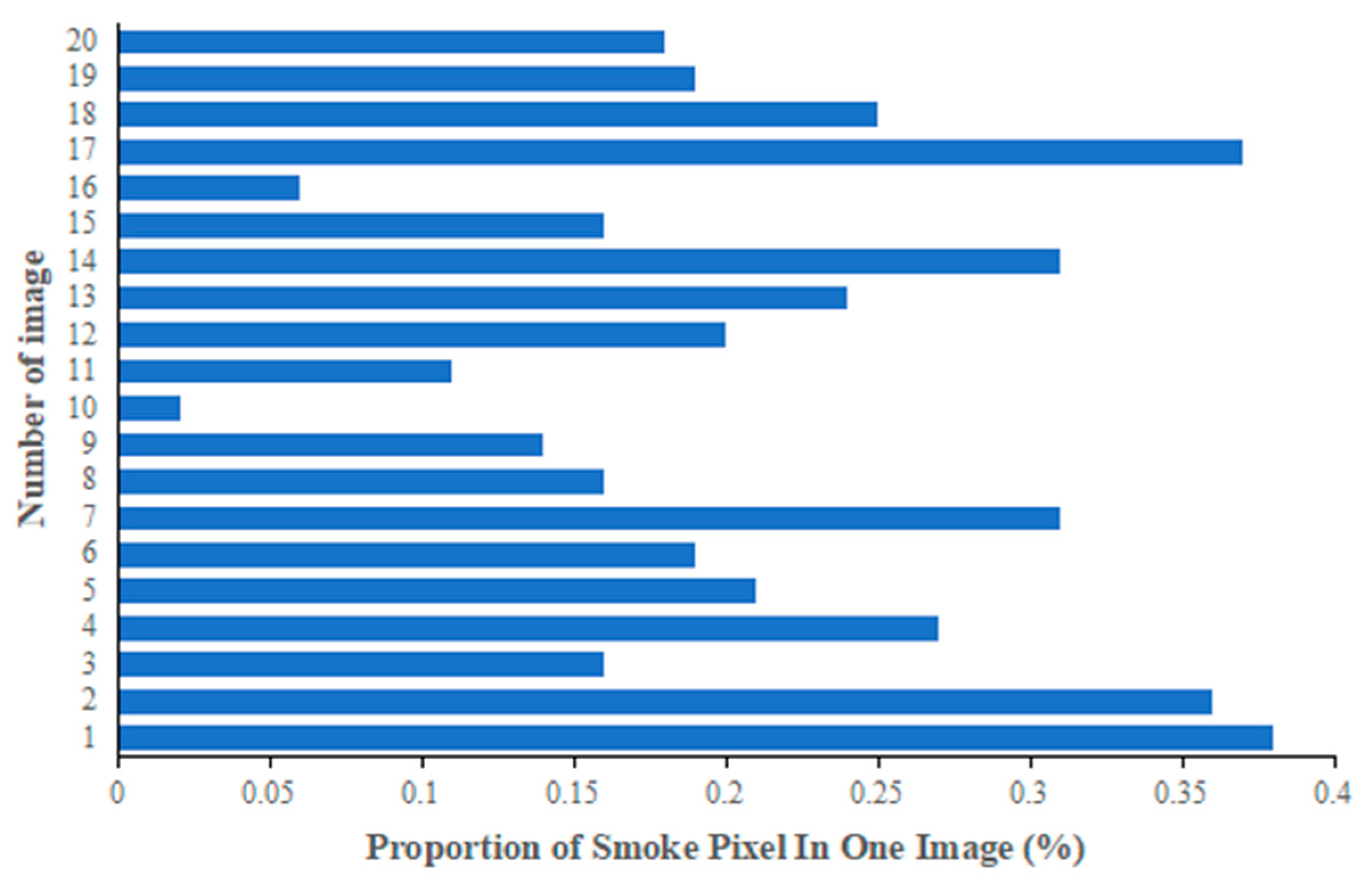
Depending on the stage of the forest fire, both the concentration and proportion of smoke pixels in a single photograph vary. At the beginning of the fire, pixels containing sparsely scattered smoke occupy a small percentage of the image; however, towards the middle of the fire, pixels containing densely spread smoke occupy nearly the entirety of the image. In order to create a more accurate recognition model, the fraction of smoke pixels in the images must be varied while studying smoke detection in early forest fires. Figure 2 depicts the percentage of smoke pixels to cropped image pixels used to form the dataset.

2.2. VIIRS Multispectral Data

Scanning imaging radiometer VIIRS (Visible Infrared Imaging Radiometer Suite) captures radiation images of the Earth’s surface, atmosphere, ice, and oceans in both the visible and infrared spectrums. It is an upgrade and expansion of previous Earth Observation Series instruments like the MODIS medium-resolution imaging spectrometers and the High-Resolution Radiometer AVHRR. The VIIRS sensor data record (SDR) contains 22 channels that span visible and infrared wavelengths between 0.41 and 12.01 microns. Five of these channels are I-bands, sixteen are medium-resolution bands (M-bands), and the remaining channel is a unique panchromatic Day/Night band (DNB). In this study, we utilized one band with high resolution (I1) and four bands with moderate resolution (M3, M4, M11, M15). The parameters of the bands used in this paper are shown in Table 3.
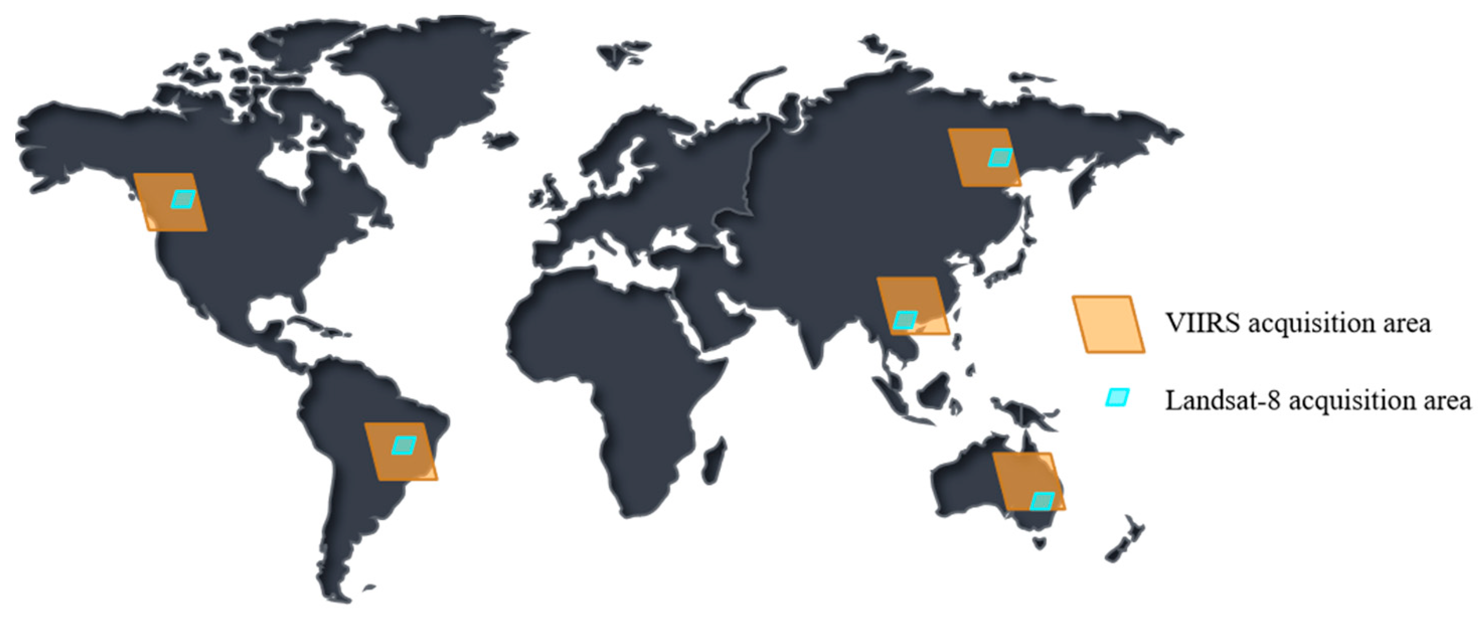
To ensure the consistency of the study area, both VIIRS and Landsat-8 images were captured at the same time and location (Figure 3). In addition, using VIIRS and Landsat-8 true color images, we manually annotated the smoke plume to establish smoke benchmark data and validate the smoke detection results. The total number of manually labeled Landsat-8 smoke pixels is 106,750,000 and the total number of VIIRS smoke pixels is 675,732.

2.3. Datasets for Smoke Detection

Smoke detection results were evaluated using the NOAA S-NPP Data Exploration (NDE) version of VIIRS level 2 aerosol products, including aerosol optical depth (AOD) and aerosol detection products (ADP) [19]. The VIIRS AOD product provides aerosol optical depth at 550 nm, which is defined as vertically integrated column total extinction at 0.55 nm. This product is derived from the Second Simulation of the Satellite Signal in the Solar Spectrum (6S) radiative transfer model. During the day, the VIIRS ADP product classifies VIIRS pixels as clear, smoke, or dust. For operational smoke detection in the ADP product, two algorithms, one based on deep blue and one on IR-visible, have been developed.
The scattering-based smoke detection algorithm (SSDA)was also used to evaluate the smoke detection results of this study. SSDA relies mainly on visible light and the blue and green bands of VIIRS. The SSDA is founded on the theory of Mie scattering, which occurs when the diameter of an atmospheric particulate is comparable to the wavelength of the scattered light. As a result of the close correspondence between smoke particulate diameters and the blue/green band wavelengths, smoke frequently causes Mie scattering in the VIIRS blue and green bands.

2.4. Datasets for Training and Testing

To create the new algorithm, smoke samples from fire-prone areas were chosen for training and validation, and the algorithm was tested globally. Images from 20 different areas were downloaded in total. To ensure consistency across the study area, the size of each study area was cropped to 150 km × 150 km. Images from Landsat-8 (30 m) were saved as 5000 × 5000 pixels. VIIRS (375 m) images were saved at 400 × 400 pixels.

2.5. Datasets for Smoke Segmentation Network

Seven Landsat-8 image bands were used in total to train the super-resolution reconstruction model: R, G, B, NIR, SWIR1, SWIR2, and TIRS1. The Landsat-8 images were cropped to 100 × 100 pixels using the sliding window method. Considering the balance of dataset type, location, and image acquisition time, a total of 100,000 100 × 100 pixel images from 20 study areas are selected in this paper to build a dataset for image super-resolution reconstruction, of which 90% are used for training and 10% for testing.

2.6. Datasets for Super-Resolution Network

We used Landsat-8 images in five bands to train the smoke segmentation model: R, G, B, SWIR2, TIRS1. Landsat-8 images from various bands were cropped to 250 × 250 pixel sizes using a random cropping method. To ensure that 60% of the images had smoke, the other backgrounds were clouds, water bodies, vegetation, bare land, and cities, resulting in a total of 6030 sets of images screened. To reduce overfitting, it was also necessary to enhance the existing images using data enhancement techniques: images of 250 × 250 pixel size were randomly cropped to 240 × 240 pixels and mirrored vertically and horizontally. Finally, a total of 54,270 images of 240 × 240 pixels were selected to build a dataset for smoke segmentation, where 70% of the images were used for training, 15% for validation, and 15% for testing.

3. Method

To accurately identify smoke on super-resolution reconstructed VIIRS images, we optimized the super-resolution reconstructed network and the smoke segmentation network in terms of smoke detection accuracy. As a result, as shown in Figure 4, we integrate the image resolution enhancement network and the smoke segmentation network in three stages. There are three parts to the training strategy: (i) domain adaptation resolution: Using the CycleGAN network, the RGB image domain of the low-resolution VIIRS (consisting of I1, M3, and M4 bands) is adjusted to the RGB image domain of Landsat-8 (consisting of R, G, and B bands). The transformed image is then fed into the following network; (ii) reconstruction network training: Using high-resolution Landsat-8 images and their downsampled images, super-resolution reconstruction network models are trained, and the trained models are used for super-resolution reconstruction of VIIRS images; (iii) smoke segmentation network training: Using high-resolution Landsat-8 images and manually annotated smoke images, the network models for smoke segmentation are trained, and the trained models are used to smoke segmentation of the super-resolution reconstructed VIIRS images.

3.1. SISR Network

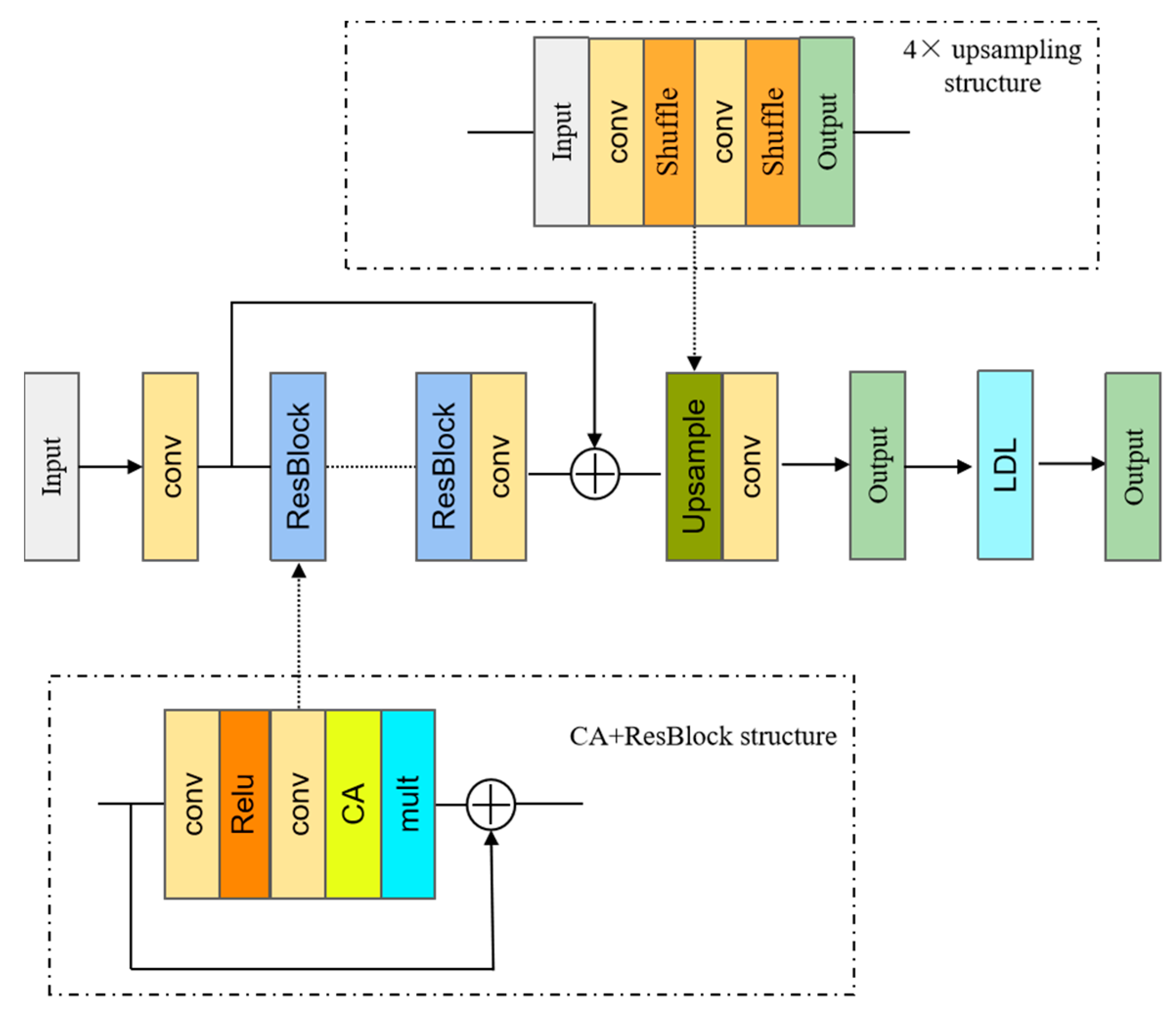
The super-resolution reconstruction network in this paper is derived from EDSR, an advanced network with ResNet architecture for single-image super-resolution. Convolution is first performed to extract image features after image input, and parameter sharing improves training efficiency. The residual blocks are used to improve the capability of feature extraction, and an increase in their number can effectively enhance the accuracy of satellite image reconstruction [27]. The residual block consists of Conv, Relu, and Mult (residual scaling) layers, which employ “skip connections” to deal with the increasing depth of the network, thereby reducing the average effective path length of the network, resolving the gradient disappearance issue and significantly accelerating the learning speed. By incorporating coarse semantic and local appearance information, the residual block with a skip connection structure also increases the network’s robustness. The Relu layer is an activation function layer that permits a subset of neurons to have a zero output. This reduces the interdependence of the parameters and creates sparsity in the network, thereby preventing overfitting. Due to the fact that an excessive number of residual blocks can result in unstable training, residual scaling is employed, i.e., the residual blocks are multiplied by a decimal number (0.1 is used in the paper) throughout the convolution process prior to summing, which can result in more stable training. After learning the image’s high-frequency characteristics, the image is reconstructed with super-resolution. A upsampled module is comprised of a convolution layer and a shuffle, with the shuffle layer completing the final upsampling through sub-pixel convolution [27]. In this paper, we chose to upsample the image by a factor of 4, because the 93.75 m VIIRS image obtained after reconstruction can effectively balance the signal loss and the higher spatial resolution requirement for smoke detection, considering that super-resolution leads to image signal loss.
The reconstruction accuracy and perceptual quality of super-resolution images are important indicators to evaluate the effect of super-resolution, and the effect of super-resolution is also directly related to the accuracy of smoke segmentation. Therefore, we add the Channel Attention (CA) mechanism and the Locally Discriminative Learning (LDL) mechanism to the EDSR network to improve the quality of super-resolution. The overall structure of the network is shown in Figure 5.

3.1.1. Channel Attention (CA)

The LR channel-wise features are treated equally by prior CNN-based SR techniques, which is not flexible enough for real-world scenarios. We take advantage of the dependencies between feature channels to direct the network’s attention to more informative features, creating a channel attention mechanism [35]. As mentioned above, residual groups and long skip connections let the main parts of the network concentrate on the principal LR features. To further improve the network’s capacity for discrimination, channel attention extracts the channel statistic from each channel.

3.1.2. Locally Discriminative Learning (LDL)

The images in the SISR results [32] have rich and realistic details with high perceptual quality. Unfortunately, details and artifacts are frequently entangled in high-frequency image components. As a result, under existing frameworks, optimizing one frequently harms the other. According to Liang et al. [32], the local variance of residuals between SISR results and ground truth HR images can be used to distinguish unpleasant artifacts from realistic details. As a result, a local discriminative learning (LDL) framework was created to penalize artifacts while preserving realistic details. The method is simple and effective enough to be easily incorporated into existing SR methods, and it has been demonstrated to be successful on the residual network ResNet [32].

3.2. Domain Adaptation

In our study, the SWIR2 and TIRS1 bands in Landsat-8 have roughly similar wavelength ranges with little domain shift to the M11 and M15 bands in VIIRS. However, it is difficult to adjust the classifier from the domain of Landsat-8 RGB images (R, G, B) to the domain of VIIRS RGB images (I1, M3, M4) using simple data enhancement techniques.
To get around this problem, a generative adversarial network was used to translate images from the source domain to the target domain. This made a lot of progress in unsupervised domain adaptation for semantic segmentation [33]. These methods based on translating images include two steps. First, it learns how to translate images from the source domain to the target domain. Second, the translated images and the labels for the corresponding source images are used to train the classifier, which will then be tested on the unlabeled source domain. When the first step reduces the domain shift, the second step can effectively make the segmentation model adapt to the target domain. The new image translation network (like CycleGAN [33]) is bidirectional. This means that when the image translation model is trained, we can usually get two image generators for the source-to-target and target-to-source directions. We can use both generators to get the best information from both directions.
Nevertheless, resolving the aforementioned issues presents a few obstacles. The transformed images and their original counterparts must have the same semantic content as the original images. Any semantic change will have an effect on our segmentation model. Therefore, we must evaluate the effect of domain adaptation on the final results of smoke segmentation.

3.3. Smoke Segmentation Network

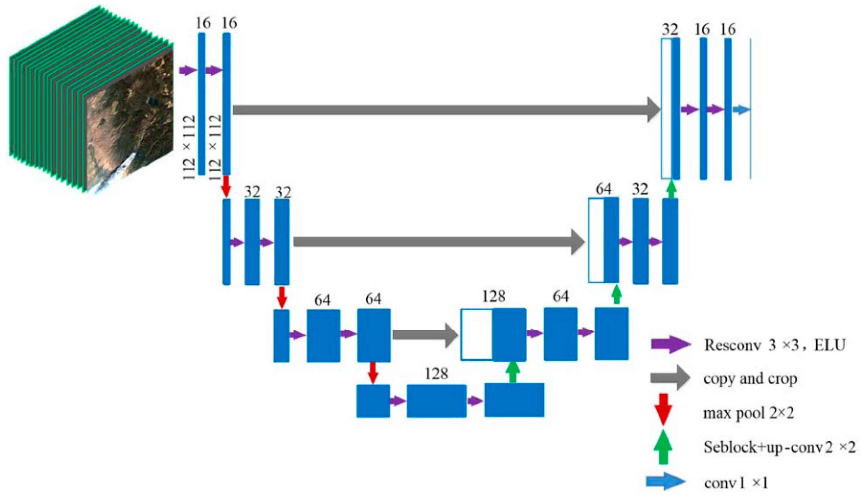
Smoke-Unet [36] (Figure 6) is used for the final segmentation task in this study. As a dense prediction problem, the classification of smoke in satellite images requires making predictions for each pixel. For segmenting smoke in satellite images, Smoke-Unet incorporates residual blocks and attention models based on the U-net network structure.
To improve the network’s feature learning capability, residual blocks are added to the convolutional blocks in order to improve feature extraction. The residual blocks with skip connection structure can improve the network’s performance and increase the robustness. The layer-skipping structure can combine coarse semantics with local appearance information. This skip feature is learned from beginning to end to improve the output’s semantic and spatial accuracy. By adjusting the weight coefficients, the focusing process can be simulated in the attention model. Focused regions can be assigned greater weight coefficients to represent the significance of the information in these regions, while other regions can be assigned smaller coefficients to filter out irrelevant information. By taking into account the varying levels of significance of information, the efficiency and precision of information processing can be significantly enhanced [36].

4. Results

In this section, we performed super-resolution reconstruction, domain adaptation, and semantic segmentation experiments on VIIRS images. By comparing the experimental results, we evaluated the performance of each network and different modules in the network, and analyzed the sensitivity of the reconstruction evaluation index, waveband, and remote sensing parameters for smoke segmentation.

4.1. Experimental Environment

The network structure uses the Keras architecture and several related image processing libraries. The programming language uses Python 3.5. The specific configuration is shown in Table 4.

4.2. Implementation Details

4.2.1. SISR Network

The input to the super-resolution reconstruction network is the Landsat-8 image. There are 7 channels of data, as shown in Table 5.
The number of residual blocks in the super-resolution model training is set to 32 and the number of filters is set to 256. During training, the back-propagation optimization algorithm uses the stochastic gradient descent (SGD) algorithm, the batch size is set to 128, and a total of 150 epochs are performed to fit the GPU memory. The initial learning rate is set to 1 × 10⁻⁴ and decreases by a factor of 2 when the validation loss is not reduced for 5 consecutive epochs. As a loss function, we use the mean absolute pixel error (L1 parametric) between the real and predicted high-resolution images. After the training is completed, the PSNR, SSIM, SRE, and PI [37] metrics are calculated for the Landsat-8 training and test sets and for each band of VIIRS.

4.2.2. CycleGAN

The input of CycleGAN network is the true color image of Landsat-8, VIIRS. After bidirectional style conversion, RGB images of Landsat-8, VIIRS are used for the smoke segmentation test.
During the model training, we cut the images and their labels into 100 × 100 pixels using the sliding window method. The back-propagation optimization algorithm uses the stochastic gradient descent (SGD) algorithm, the batch size is set to 12, and a total of 100 epochs are performed to fit the GPU memory. The learning rates for the generators, the discriminators, and the classifiers are all set to 1 × 10⁻⁴.

4.2.3. Smoke-Unet

The input of Smoke-Unet is an index of multi-channel remote sensing images and multi-remote sensing features. The 6-channel input data of Landsat-8 (R, G, B, SWIR2, AOD, BT) correspond to the smoke-sensitive bands and remote sensing indices of VIIRS (R, G, B, M11, AOD, BT), as shown in Table 6.
During the model training, the back-propagation optimization algorithm uses the stochastic gradient descent (SGD) algorithm, the learning rate is 1 × 10⁻³, the momentum is 0.9, the learning rate attenuation is 0.1, the loss function is the joint loss function, and the evaluation function is Jaccard similarity function. The batch size is 128. Considering the computing resources, there are 150 epochs in total, and shuffle is used to disrupt the order of training samples in each epoch. After each round of iteration is completed, the Jaccard coefficient, Accuracy, F1 and other indicators of the training set and the validation set are calculated.

4.3. Evaluation Indicators

4.3.1. PSNR

PSNR is the most widely used image quality assessment (IQA) method in the SISR field, which can be easily defined via the mean squared error (MSE) between the ground truth image and the reconstructed image:
P S N R = 10 · log 10 M A X 2 M S E
where M A X is the maximum possible pixel of the image. Since PSNR is highly related to MSE, a model trained with the MSE loss will be expected to have high PSNR scores. Although higher PSNR generally indicates that the construction is of higher quality, it only considers the per-pixel MSE, which makes it fail to capture the perceptual differences.

4.3.2. SSIM

SSIM is another popular assessment method that measures the similarity between two images on the perceptual basis, including structures, luminance, and contrast. Different from PSNR, which calculates absolute errors on the pixel level, SSIM suggests that there exist strong inter-dependencies among the pixels that are spatially close. These dependencies carry important information related to the structures perceptually. Thus, SSIM can be expressed as a weighted combination of three comparative measures:
S S I M I S R , I Y = l I S R , i Y α · c I S R , I Y β · s I S R , i Y γ = 2 μ I S R μ I Y + c 1 2 σ I S R σ I Y + c 2 μ I S R 2 μ I Y 2 + c 1 σ I S R 2 σ I Y 2 + c 2
where l , c , and s represent luminance, contrast, and structure between I S R and I Y , respectively.   μ I S R , μ I Y , σ I S R 2 , σ I Y 2 , σ I S R , σ I Y are the average ( μ )/variance ( σ 2 )/covariance of ( σ ) the corresponding items.

4.3.3. SRE

Depending on the scene content, some images have higher reflectance values than others, with typically higher absolute reflectance errors. To compensate for this effect, we also compute the signal to the reconstruction error ratio (SRE) as an additional error metric, which measures the error relative to the power of the signal:
S R E = 10 · log 10 μ x 2 X ^ X 2 n
where X ^ is the reconstructed band (vectorized), X is the vectorized ground truth band, and n is the number of pixels in X . μ x is the average value of X . The values of SRE are given in decibels (dB). The larger the value, the smaller the power error.

4.3.4. PI

The improvement in reconstruction accuracy is not always accompanied by an improvement in visual quality. In fact, researchers have shown that the distortion and perceptual quality are at odds with each other in some cases [32]. The perceptual quality of an image is defined as the degree to which it looks like a natural image, which has nothing to do with its similarity to any reference image. The perception index (PI), a parameter for assessing the perception quality of an image, is a combination of the reference-free image quality measure Ma [38] and NIQE [39]. The lower PI indicates the better perceptual quality of the reconstructed image.
P I = 1 2 10 M a + N I Q E

4.3.5. Jaccard Similarity Coefficient

In the field of deep learning image segmentation, the similarity coefficient is an important indicator to measure the accuracy of image segmentation. The Jaccard similarity coefficient is used in this paper to evaluate the similarity and difference between image targets. The larger the value of Jaccard, the more similar the two targets. For two sets A and B, the Jaccard coefficient is the ratio of the intersection and the union of the two, defined as:
J A , B = A B A B = A B A + B A B 0   J A , B 1

4.4. Ablation and Comparative Analysis

4.4.1. SISR

To validate the role of CA and LDL for super-resolution reconstruction, we performed ablation experiments for super-resolution reconstruction on true color images of VIIRS and other multispectral band images (M11, M15). CA denotes the integration of the original network with the channel attention mechanism, and LDL refers to the integration of the original network with LDL. The results of super-resolution reconstruction were evaluated by PSNR, SSIM, SRE, and PI metrics. To verify its validity more extensively, we compared it with other common super-resolution reconstruction networks such as VDSR and VDSen2. The comparison of the results is shown in Table 7.
As can be seen from Table 5, our super-resolution reconstructed network has been improved in PSNR, SSIM, SRE, and PI to different degrees. Compared with the original network, PSNR increases by 6.4%, SSIM increases by 1.6%, SRE increases by 6%, and PI increases by 9%. This shows that the performance of the network is better than the original network, and it can be seen from Table 6 that our network is also better than other resolution reconstruction networks.
It is worth mentioning that in the CA network, its improvement for PSNR, SSIM, and SRE is better than that of LDL, but in the PI index, CA increases rather than decreases compared with the original network. The reason for this is that details and artifacts are often entangled in the high-frequency components of the image, and CA introduces visual artifacts in the image when using high-frequency information. This is also consistent with previous studies. LDL is able to compensate for the deficiencies of CA, although it is inferior to CA in the recovery of image accuracy.

4.4.2. CycleGAN

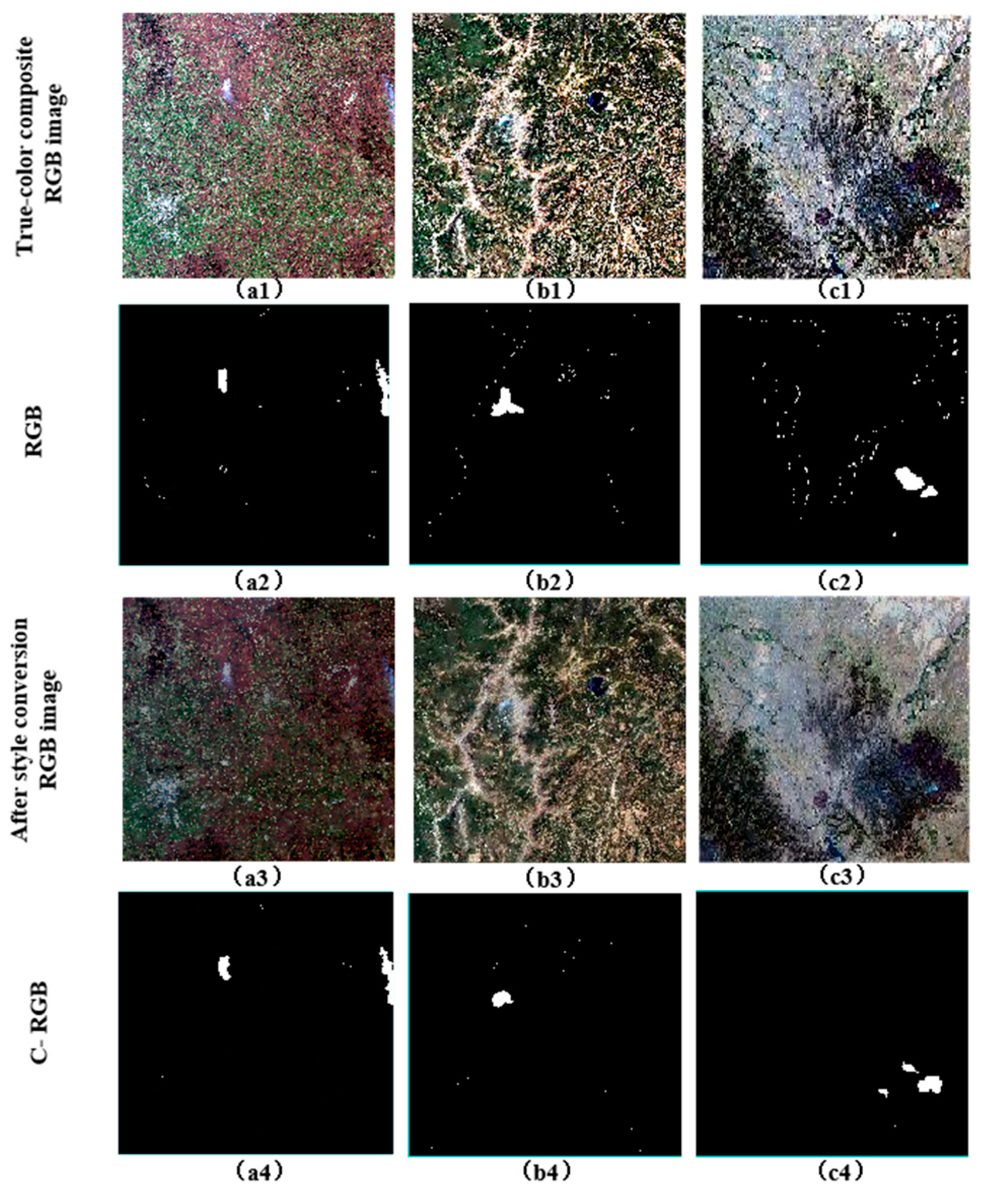
To verify whether CycleGAN can play a positive role in smoke segmentation, we conducted ablation experiments on the true color images of VIIRS. The Jaccard similarity coefficients of segmented images and VIIRS labeled images were evaluated, as well as other metrics. C-VIIRS indicates that the RGB images were CycleGAN style transformed. The comparison of the results is shown in Table 8 and Figure 7.
As can be seen from Table 6, C-VIIRS has improved in various metrics to varying degrees. The Jacaard increases by 22.1%, Precision increases by 7.8%, Recall increases by 33%, and F1 increases by 18.4%. This shows that CycleGAN network improves the generalization ability of the model and is able to solve the domain adaptation problem encountered in the text.
In Figure 7(a1), the smoke contains small areas of dense and diffused thin smoke from multiple fire initiation sites, and the land cover includes vegetation, bare soil, and cities and rivers. In Figure 7(b1), the land cover includes vegetation, bare soil, and lakes. In Figure 7(c1), the land cover includes vegetation, bare soil and cities, and cirrus clouds. As can be seen in Figure 7(a2,b2,c2), when the original VIIRS images are input, satisfactory prediction labels cannot be generated, and large misclassifications occur in the smoggy and non-smoggy regions. This also confirms the sensitivity of the segmentation model to domain shifts between the source and target domains. As can be seen in Figure 7(a4,b4,c4), the prediction labels are significantly improved when inputting the style-shifted VIIRS images, and are able to largely identify the smoke regions, including both dense and thin smoke. The misclassification of other regions is also significantly reduced.

4.5. Sensitivity Analysis

With the increase in high-resolution images and data dimensional channels, the information redundancy generated by high dimensionality makes it difficult to effectively utilize the rich information of remote sensing images. In this section, based on the smoke segmentation model described above, the effects of different combinations of VIIRS channel data and remote sensing parameters on the segmentation results are analyzed and discussed. Before this step, all RGB images have been translated.

4.5.1. Sensitivity of Bands

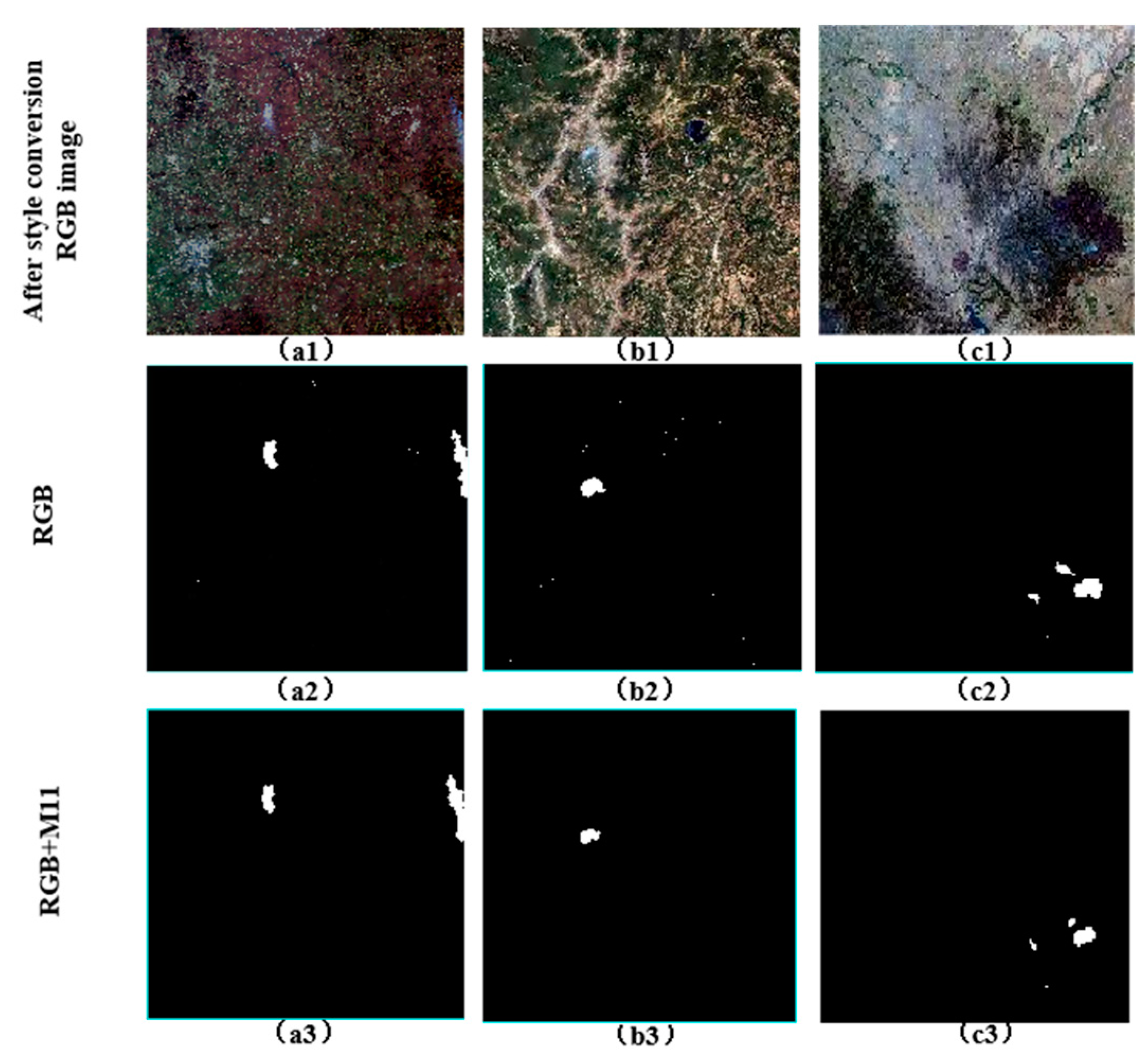
To evaluate the band sensitivity, we conducted segmentation experiments on the VIIRS dataset with different combinations of bands. The distribution of data sources is shown in Table 9.
As can be seen in Table 10 and Figure 8, the smoke segmentation results are further improved when the input bands are RGB and M11. Using RGB and M11 inputs results in a 9.4% increase in the Jaccard compared to the RGB channel only. In addition to this, the addition of the M11 band makes all misclassifications in areas away from the smoke disappear. In the near-smoke region, there is also a further effect on the discrimination of thin smoke and other land cover types. Mid-wave infrared is more sensitive to smoke detection because there is experimental evidence that smoke is less reflective in the M11 (2225–2275 nm) and SWIR (2110–2290 nm) wavelength ranges, allowing smoke particles to be distinguished from other particles [34,36].

4.5.2. Sensitivity of Remote Sensing Parameters

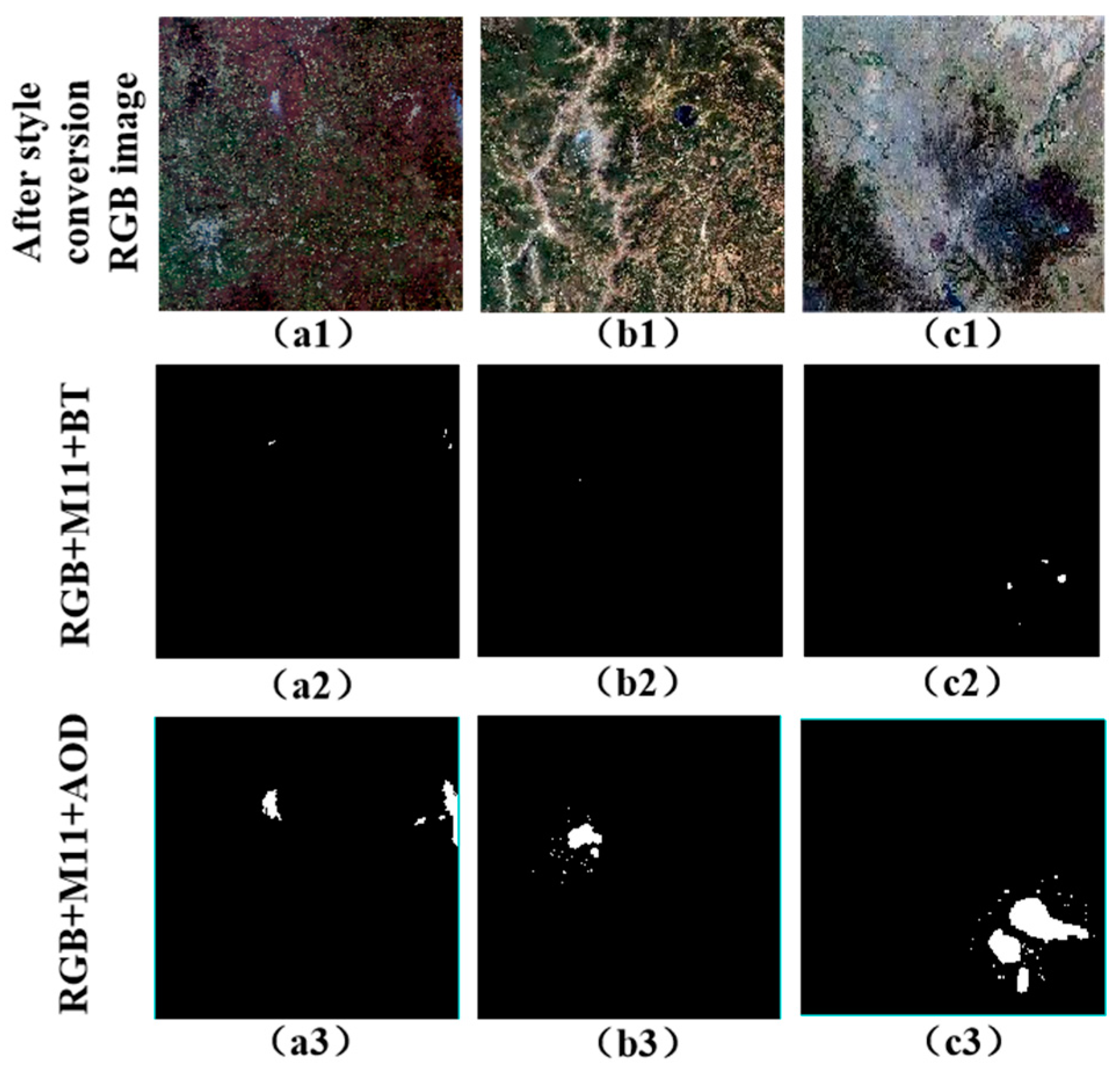
To evaluate the sensitivity of remote sensing feature indicators BT and AOD to smoke segmentation, we combined BT and AOD with RGB + M11, respectively, as shown in Table 11 and Figure 9 to evaluate their effects on smoke segmentation.
As can be seen in Figure 9, BT helps to identify high temperature anomalies, but can lead to insufficient segmentation of smoke pixels. In Figure 9(a3,b3,c3), a large number of smoke pixels that cannot be identified through vision are segmented. This may be due to the fact that forest fire smoke contains a large amount of carbon oxides and nitrogen oxides, which increase the concentration and spread of aerosols in the area. Therefore, it can be concluded that when AOD is added as an input to RGB + M11, the segmented smoke pixels are significantly increased. However, compared to the labeled image, these added smoke pixels are segmented by mistake. Therefore, the use of AOD cannot increase smoke detection accuracy in terms of data assessment criteria of segmentation.

4.5.3. Sensitivity of SISR

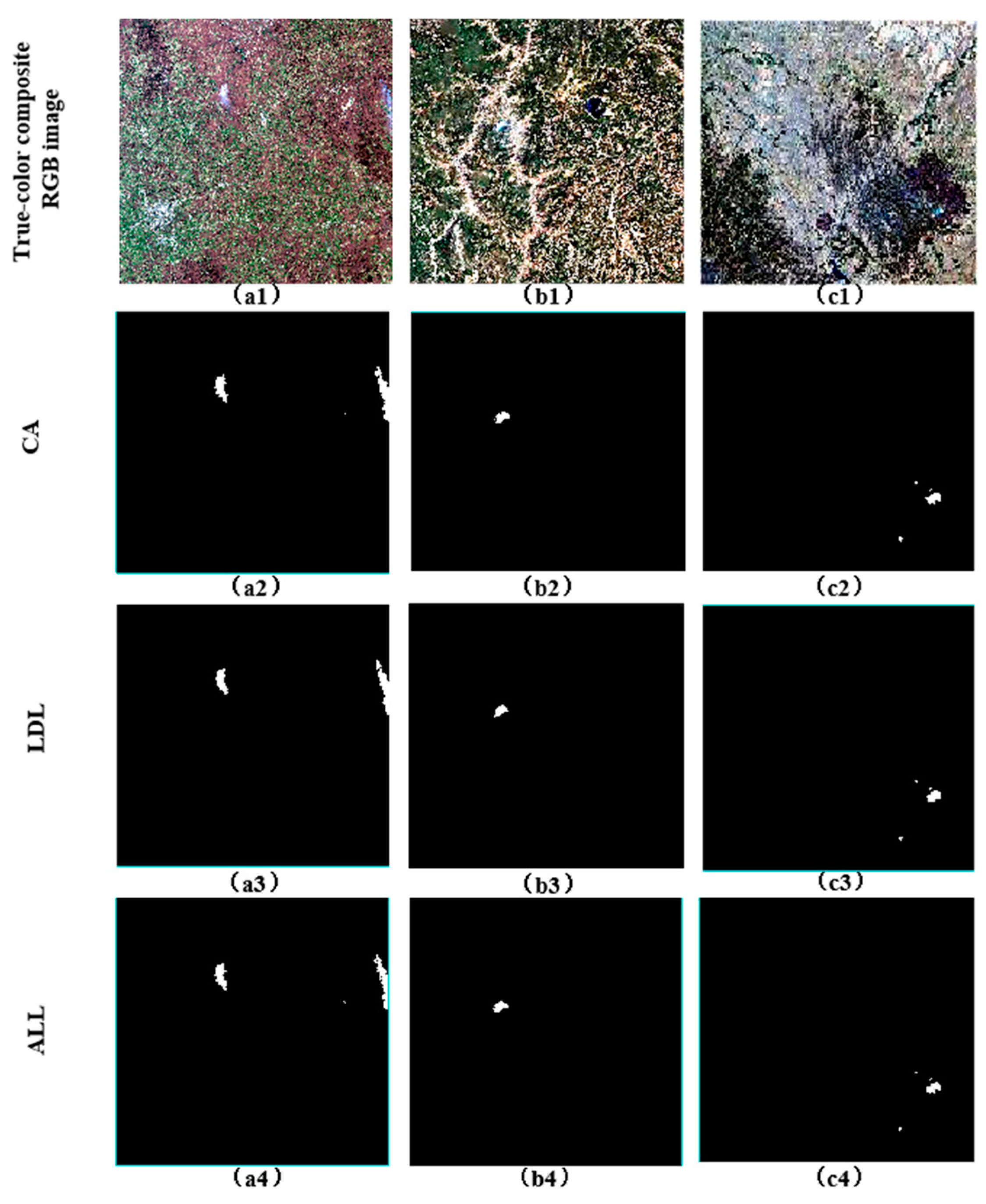
Since the ultimate goal of super-resolution reconstruction is to be able to accurately segment the smoke on low spatial resolution satellite images and try to achieve the segmentation effect of high spatial resolution satellite images. Therefore, in order to verify the contribution of each reconstruction module to the smoke segmentation, we took the reconstructed images with different super-resolution models and performed the segmentation experiments separately. The input bands were all RGB + M11. The Jaccard similarity coefficients of the segmented images, Landsat-8 downsampled images, were evaluated. Since the VIIRS image was reconstructed by a factor of 4, the resolution reached 93.75 m. To match, the Landsat-8 image resolution was downsampled to 93.75 m. The results are compared as shown in Table 12 and Figure 10—where CA represents the super-resolution reconstructed network model with added channel attention mechanism, LDL represents the super-resolution reconstructed network model with added local discrimination learning mechanism, and ALL represents the super-resolution reconstructed network model integrating CA and LDL.
As can be seen from Table 12, the super-resolution reconstruction can effectively improve the smoke segmentation accuracy of the low-resolution satellite images. Compared with the image without super-resolution, the reconstructed image Jacaard increased by 31.8%, which means that the prediction results on the low-resolution image have been able to basically approach the prediction results on the high-resolution image. This is sufficient to achieve the goal of detecting early forest fire smoke on satellites with high temporal resolution and low spatial resolution. Furthermore, we found that LDL is less elevated than CA for reconstruction efficacy.
By Figure 10(a4,b4,c4), we find that the final smoke segmentation results are close to Figure 10(a2,b2,c2). Since CA performs well in reconstruction accuracy, while LDL focuses more on perceptual quality improvement, reconstruction accuracy is more important than reconstructed perceptual quality when performing segmentation tasks.

4.6. Comparison of Smoke Segmentation

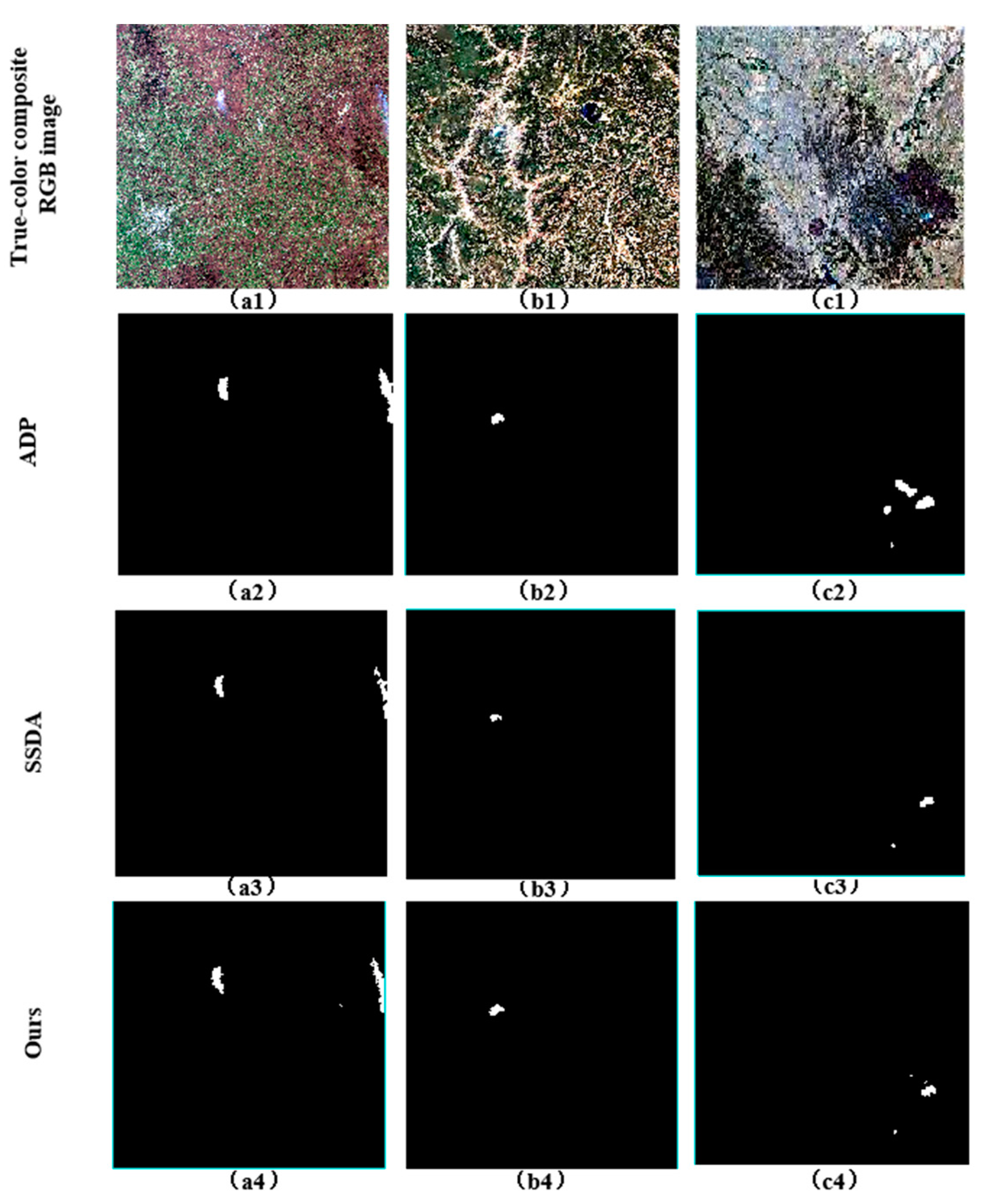
To further validate the performance of our proposed smoke recognition method, we compared it with the existing smoke recognition methods based on VIIRS images. The results are shown in Figure 11.
As can be seen in Figure 11, the boundaries of the smoke are more clearly defined in our method compared to other methods and are well distinguished from other landforms. Due to the improved resolution, some tiny smoke that is not easily recognized on the original image with low resolution is identified, as in Figure 11(a4). The accurate identification of thin smoke areas is also a great contribution compared to the latest SSDA method. We found that the ADP method also uses the AOD index, which has high smoke recognition accuracy, and more appropriately uses the AOD remote sensing index. This leads to the conclusion that the AOD index is more suitable for smoke identification in combination with other smoke detection algorithms.

5. Discussion

In order to test the practical application capability of the smoke recognition method based on remote sensing super-resolution reconstruction images, smoke segmentation tests were conducted on 20 sets of Landsat-8 images with different channel combinations, VIIRS images under different channel combinations after domain adaptation, and VIIRS super-resolution images after domain adaptation, and the segmentation results were compared with Landsat-8, VIIRS manually labeled smoke areas in terms of Jaccard similarity coefficients and the smoke areas segmented by different images. The results are shown in Table 13—where C-VIIRS indicates the result after image domain adaptation, SR-VIIRS indicates the result after image super-resolution reconstruction, and each data is taken as the average of 20 images.
As can be seen from Table 13, in the case of different channel combinations of input Landsat-8, the Jacaard similarity coefficient between the segmentation results and the manually labeled Landsat-8 smoke regions were 0.644 and 0.748, respectively, confirming that the Smoke-Unet network can effectively segment the most smoke regions. The addition of the SWIR2 band to the Landsat-8 RGB band can effectively increase the accuracy of smoke segmentation, which is also consistent with the results of previous studies. In the case of different channel combinations of VIIRS after adaptation of the input domain, the Jacaard similarity coefficient between the segmentation results and the manually labeled VIIRS smoke region was 0.697 and 0.763, respectively, confirming that Smoke-Unet network is also applicable to the VIIRS images after domain adaptation. The addition of the M11 band to the C-VIIRS RGB band can also effectively increase the accuracy of smoke segmentation, confirming the effectiveness of the M11 band in the deep learning method for smoke segmentation of VIIRS images. With the input of the super-resolution RGB image of VIIRS after domain adaptation and the M11 band, the segmentation results are similar to those of the manually labeled Landsat-8 smoke region and the Jacaard similarity coefficient is 0.742, which is already very close to the Jacaard similarity coefficient of 0.748 compared to the input of the Landsat-8 RGB+SWIR2 band. In addition, the predicted smoke area of 3598.01 km2 is also close to the Landsat-8 RGB + SWIR2 prediction of 3646.05 km2.

6. Conclusions

This paper proposes a low spatial resolution satellite remote sensing image smoke detection method with an integrated image super resolution reconstruction network and a smoke segmentation network in order to make use of high temporal resolution (24 h) but low spatial resolution (375 m), accurate and timely detection of early forest fire smoke, and achieve the effect of using high spatial resolution satellite smoke detection. The first step was to create a multispectral remote sensing smoke dataset with various years, seasons, geographies, and land cover types. The second part of this research proposed a super-resolution network of satellite remote sensing images, which combines the super-resolution reconstruction network with a channel attention mechanism and an artefact removal module. Experimental validation was made in comparison to previous approaches. Thirdly, experimental analysis was implemented to determine the effects of the super-resolution reconstruction module on the results of smoke segmentation as well as the sensitivity of various band combinations and remote sensing indices of multispectral data. The outcomes demonstrate that with a Jaccard index of 0.742, the smoke segmentation result of the satellite image (93.75 m) following the semantic segmentation is remarkably similar to the result of the high-resolution satellite image (30 m). The domain offset issue that arises during the smoke segmentation of remote sensing images based on super-resolution reconstruction is also resolved by deep domain adaptation. Last but not least, the M11 band for VIIRS images is a sensitive band for smoke segmentation utilizing deep learning algorithms, which can significantly aid in smoke pixel segmentation in VIIRS images. Super-resolution reconstruction of remote sensing images’ accuracy is more crucial for the task of smoke segmentation than the reconstruction’s perceptual quality, and it is also more sensitive to smoke segmentation.
However, the distortion of remote sensing signals generated by super-resolution might result in a sequence of errors in subsequent data processing. Secondly, the explanation for the favorable effect of sensitive bands on smoke detection needs to be researched further, which will also aid in the discovery of new remote sensing parameters suitable for smoke detection. Furthermore, studies on how to combine remote sensing characteristics while utilizing deep learning algorithms to segment smoke more precisely in remote sensing images and employ smoke areas for fire spot identification, smoke pollution assessment, and analysis are needed.

Author Contributions

Conceptualization, H.L., C.Z., Y.T. and X.L.; methodology, H.L.; software, H.L. and X.L.; validation, H.L.; formal analysis, H.L. and J.Z.; investigation, H.L.; resources, H.L.; data curation, H.L., X.L. and J.Z.; writing—original draft preparation, H.L., X.L. and J.Z.; writing—review and editing, H.L., W.C., C.Z. and X.L.; visualization, H.L.; supervision, W.C.; project administration, H.L.; funding acquisition, C.Z. All authors have read and agreed to the published version of the manuscript.

Funding

This research was funded by the National Natural Science Foundation of China, grant number 31971668.

Data Availability Statement

Data available on request due to restrictions of privacy.

Conflicts of Interest

The authors declare no conflict of interest.

References

  1. Roberts, D.A.; Dennison, P.E.; Gardner, M.E.; Hetzel, Y.; Ustin, S.L.; Lee, C.T. Evaluation of the potential of Hyperion for fire danger assessment by comparison to the Airborne Visible/Infrared Imaging Spectrometer. IEEE Trans. Geosci. Remote 2003, 41, 1297–1310. [Google Scholar] [CrossRef]
  2. Yu, Z.Z. Forest Management, 2nd ed.; China Forestry Publishing House: Beijing, China, 1993. [Google Scholar]
  3. Hu, H.Q. Fire Ecology and Management; China Forestry Publishing House: Beijing, China, 2005. [Google Scholar]
  4. Chowdhury, E.H.; Hassan, Q.K. Operational perspective of remote sensing-based forest fire danger forecasting systems. ISPRS J. Photogramm. 2015, 104, 224–236. [Google Scholar] [CrossRef]
  5. Molina-Pico, A.; Cuesta-Frau, D.; Araujo, A.; Alejandre, J.; Rozas, A. Forest monitoring and wildland early fire detection by a hierarchical wireless sensor network. J. Sens. 2016, 2016, 8325845. [Google Scholar] [CrossRef]
  6. Di Biase, V.; Laneve, G. Geostationary sensor based forest fire detection and monitoring: An improved version of the SFIDE algorithm. Remote Sens. 2018, 10, 741. [Google Scholar] [CrossRef]
  7. Keywood, M.; Kanakidou, M.; Stohl, A.; Dentener, F.; Grassi, G.; Meyer, C.P.; Torseth, K.; Edwards, D.; Thompson, A.M.; Lohmann, U.; et al. Fire in the air: Biomass burning impacts in a changing climate. Crit. Rev. Environ. Sci. Technol. 2013, 43, 40–83. [Google Scholar] [CrossRef]
  8. Hirsch, K.G.; Corey, P.N.; Martell, D.L. Using expert judgment to model initial attack fire crew effectiveness. For. Sci. 1998, 44, 539–549. [Google Scholar]
  9. Kaufman, Y.J.; Tanré, D.; Boucher, O. A satellite view of aerosols in the climate system. Nature 2002, 419, 215–223. [Google Scholar] [CrossRef]
  10. Ismanto, H.; Hartono, H.; Marfai, M.A. Smoke detections and visibility estimation using Himawari_8 satellite data over Sumatera and Borneo Island Indonesia. Spat. Inf. Res. 2019, 27, 205–216. [Google Scholar] [CrossRef]
  11. Ghirardelli, J.E.; Glahn, B. The Meteorological Development Laboratory’s aviation weather prediction system. Weather Forecast. 2010, 25, 1027–1051. [Google Scholar] [CrossRef]
  12. Brook, R.D.; Rajagopalan, S.; Pope, C.A., III; Brook, J.R.; Bhatnagar, A.; Diez-Roux, A.V.; Holguin, F.; Hong, Y.; Luepker, R.V.; Mittleman, M.A. Particulate matter air pollution and cardiovascular disease: An update to the scientific statement from the American Heart Association. Circulation 2010, 121, 2331–2378. [Google Scholar] [CrossRef]
  13. Reid, C.E.; Jerrett, M.; Petersen, M.L.; Pfister, G.G.; Morefield, P.E.; Tager, I.B.; Raffuse, S.M.; Balmes, J.R. Spatiotemporal prediction of fine particulate matter during the 2008 northern California wildfires using machine learning. Environ. Sci. Technol. 2015, 49, 3887–3896. [Google Scholar] [CrossRef] [PubMed]
  14. Brey, S.J.; Ruminski, M.; Atwood, S.A.; Fischer, E.V. Connecting smoke plumes to sources using Hazard Mapping System (HMS) smoke and fire location data over North America. Atmos. Chem. Phys. 2018, 18, 1745–1761. [Google Scholar]
  15. Akimoto, H. Global air quality and pollution. Science 2003, 302, 1716–1719. [Google Scholar] [CrossRef] [PubMed]
  16. Kumar, S.S.; Roy, D.P. Global operational land imager Landsat-8 reflectance-based active fire detection algorithm. Int. Digit. Earth 2018, 11, 154–178. [Google Scholar] [CrossRef]
  17. Wang, Y.; Zhang, J.; Zhang, H.; Xie, W.; Aruhasi, W.N. Application of MODIS AOD Products to Monitoring Forest Fire in Forest Area of Southwestern China. Arid Meteorol. 2018, 36, 820–827. [Google Scholar]
  18. Tian, X.P.; Liu, Q.; Song, Z.W.; Dou, B.C.; Li, X.H. Aerosol optical depth retrieval from Landsat 8 OLI images over urban areas supported by MODIS BRDF/Albedo Data. IEEE Geosci. Remote Sens. Lett. 2018, 15, 976–980. [Google Scholar] [CrossRef]
  19. Xiao, Q.; Zhang, H.; Choi, M.; Li, S.; Kondragunta, S.; Kim, J.; Holben, B.; Levy, R.C.; Liu, Y. Evaluation of VIIRS, GOCI, and MODIS Collection 6 AOD retrievals against ground sunphotometer observations over East Asia. Atmos. Chem. Phys. 2016, 16, 1255–1269. [Google Scholar] [CrossRef]
  20. Wang, Q.; Shi, W.; Li, Z.; Atkinson, P.M. Fusion of Sentinel-2 images. Remote Sens. Environ. 2016, 187, 241–252. [Google Scholar] [CrossRef]
  21. Santurri, L.; Aiazzi, B.; Baronti, S.; Carlà, R. Influence of spatial resolution on pan-sharpening results. In Proceedings of the 2012 IEEE International Geoscience and Remote Sensing Symposium (IGARSS), Munich, Germany, 22–27 July 2012; pp. 5446–5449. [Google Scholar]
  22. Zou, Z.; Shi, Z. Ship detection in spaceborne optical image with SVD networks. IEEE Trans. Geosci. Remote 2016, 54, 5832–5845. [Google Scholar] [CrossRef]
  23. Tatem, A.J.; Lewis, H.G.; Atkinson, P.M.; Nixon, M.S. Super-resolution target identification from remotely sensed images using a Hopfield neural network. IEEE Trans. Geosci. Remote 2001, 39, 781–796. [Google Scholar] [CrossRef]
  24. Cheng, J.; Kuang, Q.; Shen, C.; Liu, J.; Tan, X.; Liu, W. ResLap: Generating high-resolution climate prediction through image super-resolution. IEEE Access 2020, 8, 39623–39634. [Google Scholar] [CrossRef]
  25. Dong, C.; Loy, C.C.; He, K.; Tang, X. Learning a deep convolutional network for image super-resolution. In Lecture Notes in Computer Science; Fleet, D., Pajdla, T., Schiele, B., Tuytelaars, T., Eds.; Springer: Cham, Switzerland, 2014; Volume 8692, pp. 184–199. [Google Scholar]
  26. Zhang, Y.; Tian, Y.; Kong, Y.; Zhong, B.; Fu, Y. Residual dense network for image super-resolution. In Proceedings of the IEEE Conference on Computer Vision and Pattern Recognition (CVPR), Salt Lake City, UT, USA, 18–23 June 2018; pp. 2472–2481. [Google Scholar]
  27. Lanaras, C.; Bioucas-Dias, J.; Galliani, S.; Baltsavias, E.; Schindler, K. Super-resolution of Sentinel-2 images: Learning a globally applicable deep neural network. ISPRS J. Photogramm. 2018, 146, 305–319. [Google Scholar] [CrossRef]
  28. Blau, Y.; Michaeli, T. The perception-distortion tradeoff. In Proceedings of the IEEE Conference on Computer Vision and Pattern Recognition (CVPR), Salt Lake City, UT, USA, 18–23 June 2018; pp. 6228–6237. [Google Scholar]
  29. Ledig, C.; Theis, L.; Huszár, F.; Caballero, J.; Cunningham, A.; Acosta, A.; Aitken, A.; Tejani, A.; Totz, J.; Wang, Z.; et al. Photo-realistic single image super-resolution using a generative adversarial network. In Proceedings of the IEEE Conference on Computer Vision and Pattern Recognition (CVPR), Honolulu, HI, USA, 16–21 July 2017; pp. 4681–4690. [Google Scholar]
  30. Yu, Y.; Li, X.; Liu, F. E-DBPN: Enhanced deep back-projection networks for remote sensing scene image superresolution. IEEE Trans. Geosci. Remote 2020, 58, 5503–5515. [Google Scholar] [CrossRef]
  31. Niu, B.; Wen, W.; Ren, W.; Zhang, X.; Yang, L.; Wang, S.; Zhang, K.; Cao, X.; Shen, H. Single image super-resolution via a holistic attention network. In Computer Vision—ECCV 2020; Vedaldi, A., Bischof, H., Brox, T., Frahm, J.M., Eds.; Springer: Cham, Switzerland, 2020; Volume 12357, pp. 191–207. [Google Scholar]
  32. Liang, J.; Zeng, H.; Zhang, L. Details or artifacts: A locally discriminative learning approach to realistic image super-resolution. In Proceedings of the IEEE/CVF Conference on Computer Vision and Pattern Recognition (CVPR), New Orleans, LA, USA, 18–24 June 2022; pp. 5657–5666. [Google Scholar]
  33. Tuia, D.; Persello, C.; Bruzzone, L. Domain adaptation for the classification of remote sensing data: An overview of recent advances. IEEE Geosci. Remote Sens. Mag. 2016, 4, 41–57. [Google Scholar] [CrossRef]
  34. Lu, X.; Zhang, X.; Li, F.; Cochrane, M.A.; Ciren, P. Detection of fire smoke plumes based on aerosol scattering using VIIRS data over global fire-prone regions. Remote Sens. 2021, 13, 196. [Google Scholar] [CrossRef]
  35. Yuan, Q.; Wei, Y.; Meng, X.; Shen, H.; Zhang, L. A multiscale and multidepth convolutional neural network for remote sensing imagery pan-sharpening. IEEE J. Sel. Top. Appl. Earth Obs. Remote Sens. 2018, 11, 978–989. [Google Scholar] [CrossRef]
  36. Wang, Z.; Yang, P.; Liang, H.; Zheng, C.; Yin, J.; Tian, Y.; Cui, W. Semantic segmentation and analysis on sensitive parameters of forest fire smoke using smoke-unet and landsat-8 imagery. Remote Sens. 2022, 14, 45. [Google Scholar] [CrossRef]
  37. Li, J.; Pei, Z.; Zeng, T. From beginner to master: A survey for deep learning-based single-image super-resolution. arXiv 2021, arXiv:2109.14335. [Google Scholar]
  38. Ma, C.; Yang, C.Y.; Yang, X.; Yang, M.H. Learning a no-reference quality metric for single-image super-resolution. Comput. Vis. Image Underst. 2017, 158, 1–16. [Google Scholar] [CrossRef]
  39. Mittal, A.; Soundararajan, R.; Bovik, A.C. Making a “completely blind” image quality analyzer. IEEE Signal Process. Lett. 2012, 20, 209–212. [Google Scholar] [CrossRef]
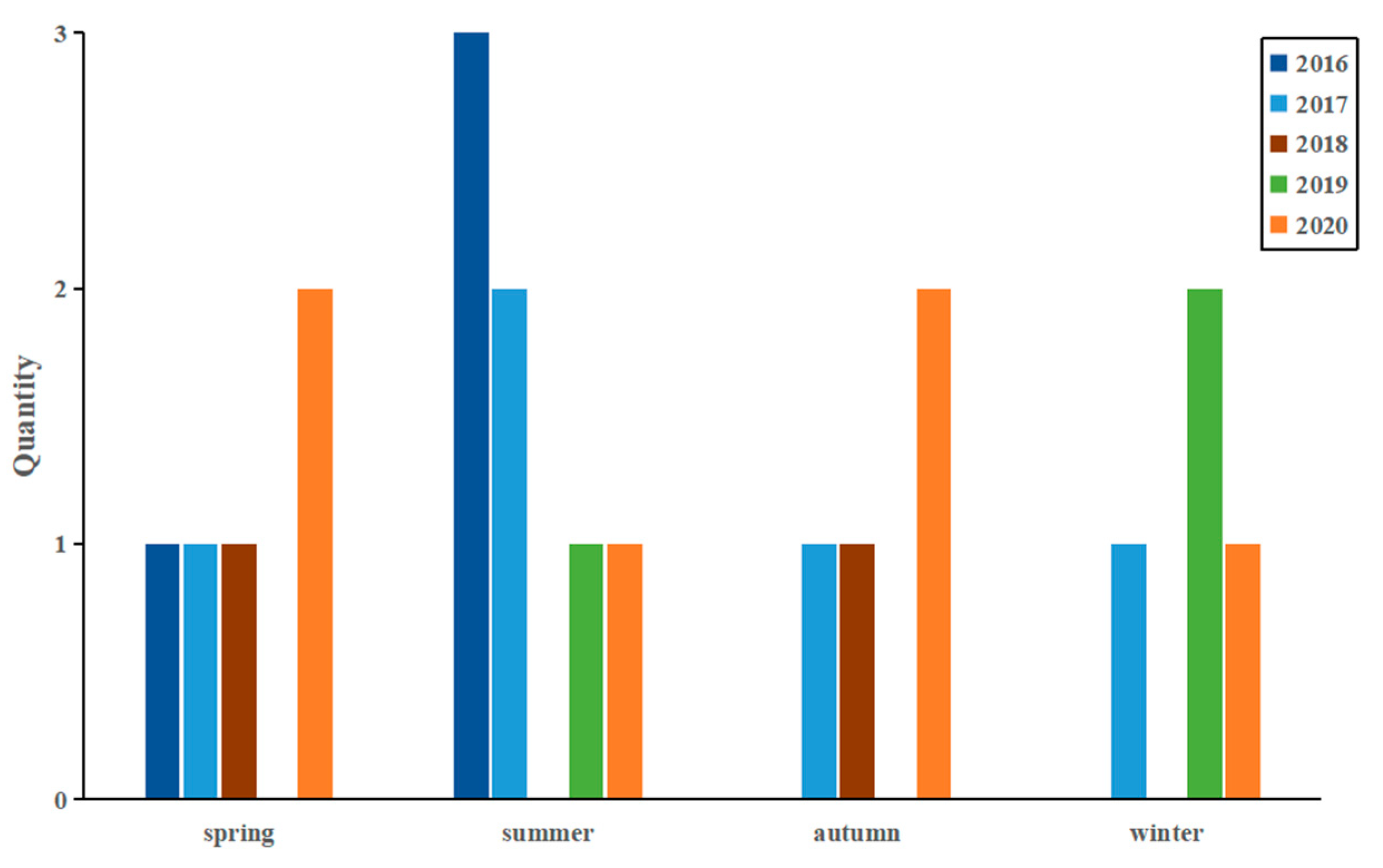
Figure 1. Seasonal statistics of fire occurrence.
Remotesensing 15 04180 g001
Figure 2. The proportion of smoke pixels of different images.
Remotesensing 15 04180 g002
Figure 3. Image acquisition area.
Remotesensing 15 04180 g003
Figure 4. Overall network structure.
Remotesensing 15 04180 g004
Figure 5. The architecture of the proposed reconstructed networks.
Remotesensing 15 04180 g005
Figure 6. Smoke-Unet [36].
Remotesensing 15 04180 g006
Figure 7. The first row shows the RGB image composed of the true color of the smoke plume. The third row shows the RGB image after the style conversion. The second and fourth rows show the smoke segmentation results for the input of different RGB images, with the smoke pixels represented in white: (a1a4) Western United States, 15 August 2020; (b1b4) Liangshan region, China, 21 May 2019; (c1c4) Southern Australia, 7 February 2019.
Remotesensing 15 04180 g007
Figure 8. The comparative segmentation result of different bands combination. The first row (a1,b1,c1) shows the RGB image that shows the stylized conversion. The second (a2,b2,c2) and third (a3,b3,c3) rows show the smoke segmentation results for images with different channel combinations input, with smoke pixels represented in white.
Remotesensing 15 04180 g008
Figure 9. The comparative segmentation result of different remote sensing parameters. The first row (a1,b1,c1) shows the RGB image that shows the stylized conversion. The second (a2,b2,c2) and third (a3,b3,c3) rows show the smoke segmentation results for images with different remote sensing parameters combinations input, with smoke pixels represented in white.
Remotesensing 15 04180 g009
Figure 10. The comparative segmentation result of different reconstruction modules. The first row (a1,b1,c1) shows the original RGB image displayed. The other rows (a2,b2,c2) (a3,b3,c3) (a4,b4,c4) are the results of the smoke segmentation of the image after reconstructing the model at different resolutions, and the smoke pixels are shown in white.
Remotesensing 15 04180 g010
Figure 11. The comparative segmentation result of different methods. The first row (a1,b1,c1) shows the original RGB image displayed. All other rows (a2,b2,c2) (a3,b3,c3) (a4,b4,c4) show the smoke segmentation results for different smoke recognition methods, with smoke pixels shown in white.
Remotesensing 15 04180 g011
Table 1. Landsat-8 Satellite Parameters.
Payload NameBand NumberBand NameSpectral Range (nm)Resolution (m)
OIL2Blue450~51530
3Green525~60030
4Red630~68030
5NIR845~88530
6SWIR11570~165030
7SWIR22110~229030
TIRS10TIRS11060~111960
Table 2. The acquisition locations and times of imagery for selecting training samples.
Region of InterestAcquisition DateSample Types
South America2016–2018Smoke, cloud,
Vegetation, bare soil, water
Asia2016–2020Smoke, cloud,
Vegetation, bare soil
Siberia2017–2020Smoke, cloud,
Vegetation, bare soil, water
Australia2018–2020Smoke, cloud,
Vegetation, bare soil, dust
West North America2019–2020Smoke, cloud,
Vegetation, bare soil, city
Table 3. The S-NPP VIIRS bands Parameters.
Payload NameBand NameSpectral Range (nm)Resolution (m)
VIIRSI1600~680375
M3478~498750
M4545~565750
M112225~2275750
M1510,263~11,263750
Table 4. Deep learning environment configuration.
Programming EnvironmentAuxiliary LibraryHardware ConfigurationOther Software
Python3.5ShapelyCPU:[email protected] GHzENVI5.3
Tensorflow1.9Opencv2.2GPU:NVDIA TITAN XScikit_image0.12.3
CUDA8.0Tifffile0.12RAM:16 GB
cuDNN10.0Rasterio1.1.2Numba0.26.0t
Keras2.2.0h5py2.6.0
Table 5. The input to SISR network.
NumberData TypeItemBand
1Band DataMultispectral Band2–7, 10
Table 6. The input of Smoke-Unet.
NumberData TypeItemLandsat-8 BandsVIIRS Bands
1Band DataMultispectral Band2, 3, 4, 7I1, M3, M4, M11
2Remote Sensing IndexAOD/
3Remote Sensing IndexBT/
Table 7. Ablation and comparative analysis of different models.
NetworkPSNRSSIMSREPI
Original67.1530.976034.87.544
CA69.1780.990136.37.622
LDL68.7670.987535.66.613
VDSR66.0430.973334.47.561
VDSen267.9570.980335.17.932
Proposed69.3150.984736.46.868
Table 8. Ablation experiments of CycleGAN.
ImageJacaardPrecisionRecallF1
VIIRS0.5710.6600.7250.683
C-VIIRS0.6970.7120.9640.809
Table 9. Ablation experiments of different bands.
NumberData TypeData DimensionBand
1RGB3R, G, B
2RGB + M114R, G, B, M11
Table 10. The segmentation results of different bands combination.
Data TypeJacaardPrecisionRecallF1
RGB0.6970.7120.9640.809
RGB + M110.7630.7710.9750.841
Table 11. Ablation experiments of remote sensing parameters.
NumberData TypeData DimensionBand
1RGB + M11 + BT5R, G, B, M11, BT
2RGB + M11 + AOD5R, G, B, M11, AOD
Table 12. Ablation experiments of different reconstruction modules.
ModelJacaard
Smoke-Unet0.563
CA + Smoke-Unet0.737
LDL + Smoke-Unet0.695
ALL + Smoke-Unet0.742
Table 13. The segmentation results of different input images.
InputImagesSpatial ResolutionTemporal ResolutionContrast ImagesJacaardSmoke Area (km2)
Landsat-8
RGB
30 m17 dayLandsat-8 0.6443482.72
Landsat-8 RGB + SWIR230 m17 dayLandsat-8 0.7483646.05
C-VIIRS
RGB
375 m24 hVIIRS0.6973324.15
C-VIIRS RGB + M11375 m24 hVIIRS0.7633599.61
SR-VIIRS RGB + M1193.75 m24 hLandsat-80.7423598.01
Disclaimer/Publisher’s Note: The statements, opinions and data contained in all publications are solely those of the individual author(s) and contributor(s) and not of MDPI and/or the editor(s). MDPI and/or the editor(s) disclaim responsibility for any injury to people or property resulting from any ideas, methods, instructions or products referred to in the content.