
Hybrid CNN-LSTM Deep Learning for Track-Wise GNSS-R Ocean Wind Speed Retrieval


Abstract
:
1. Introduction
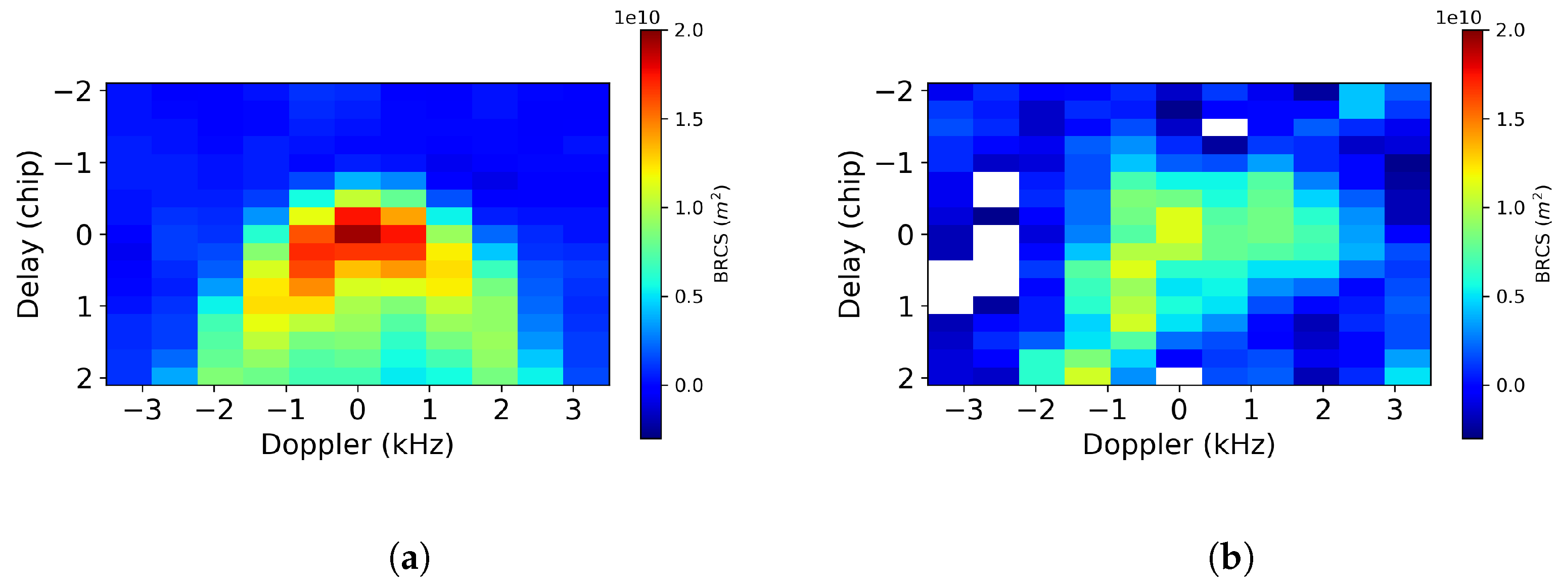
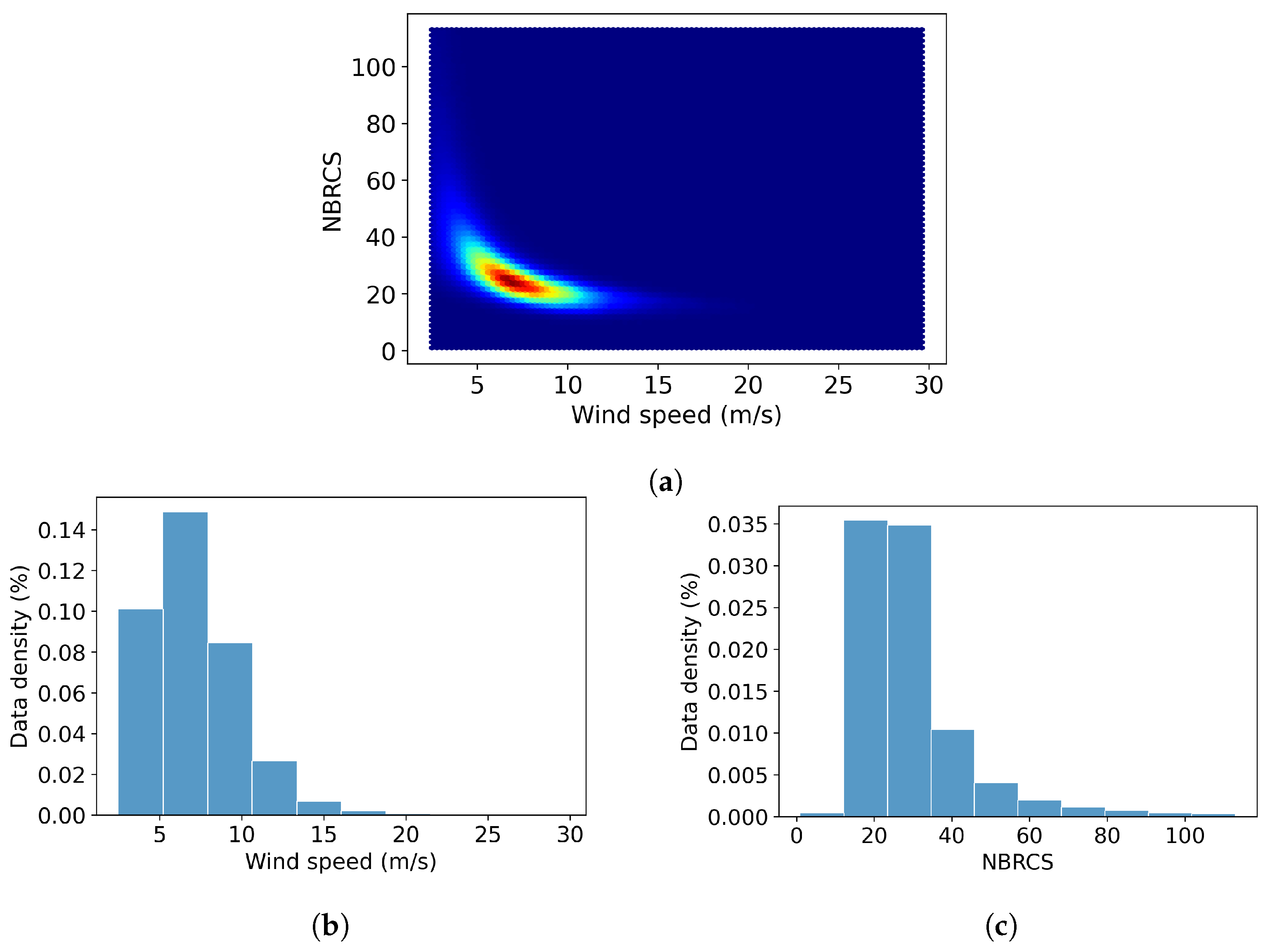
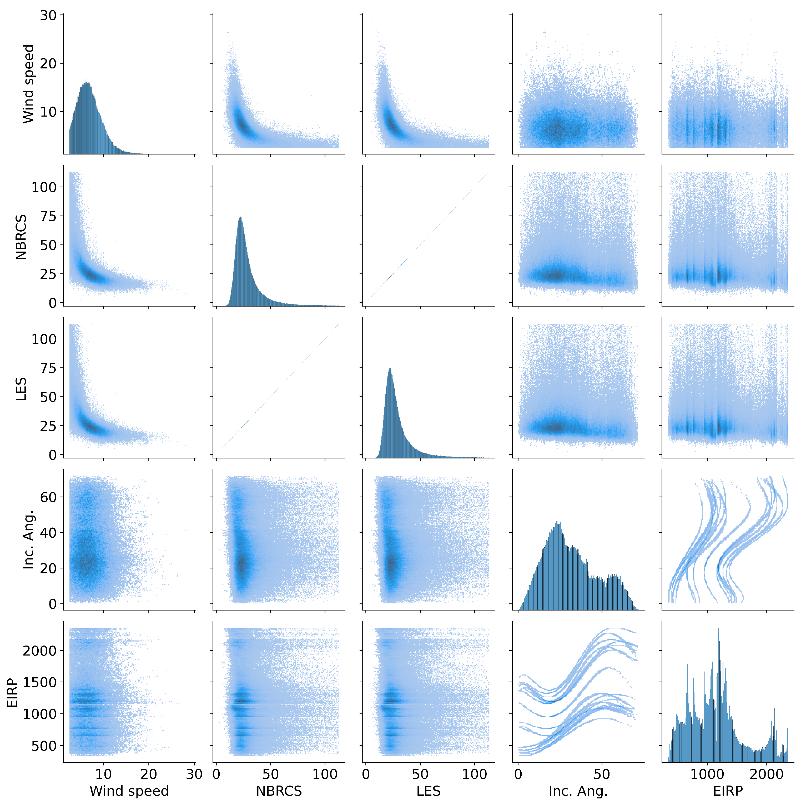
2. Dataset
3. Model Architectures
3.1. Fully Connected Layers
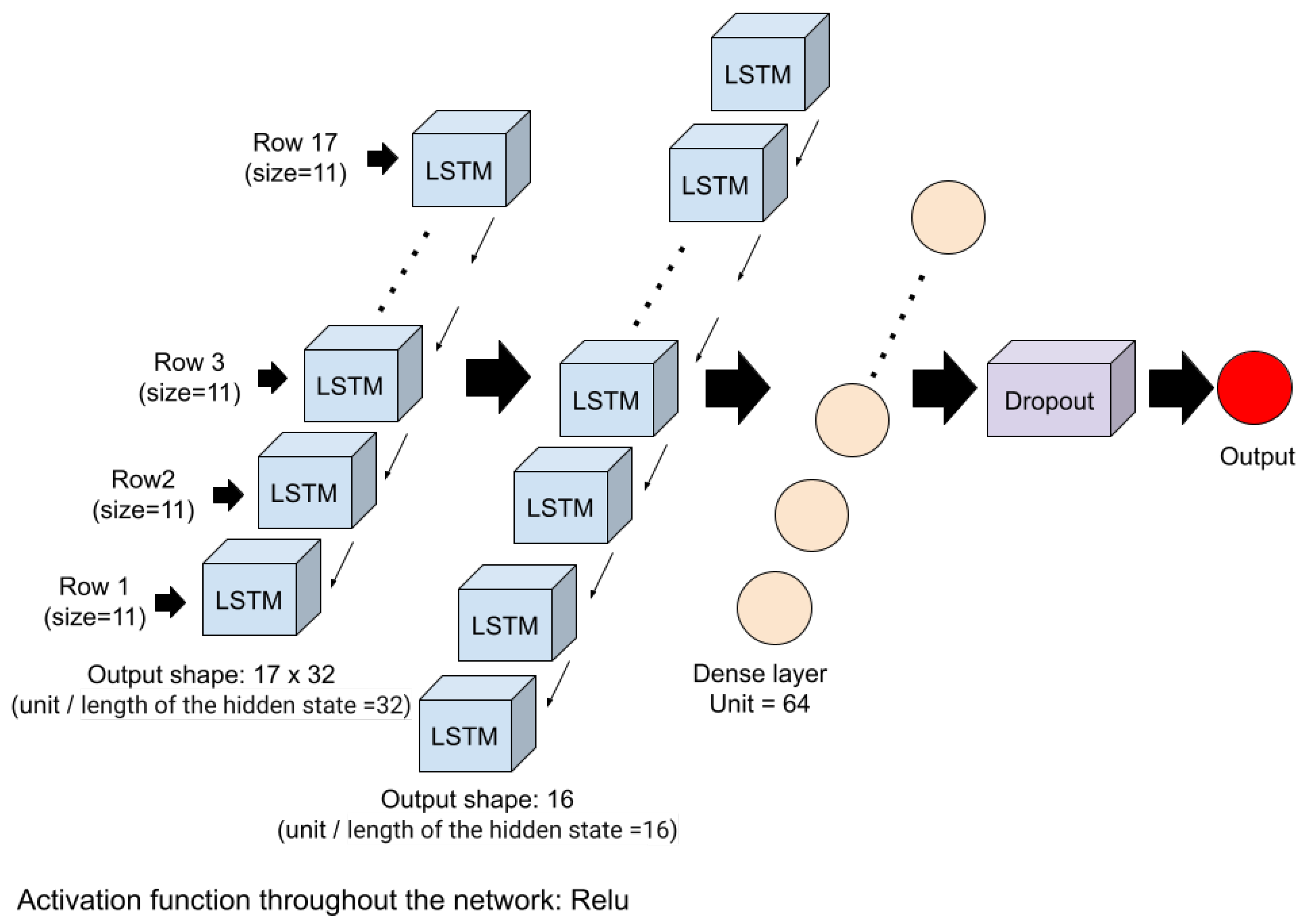
3.2. Long Short-Term Memory
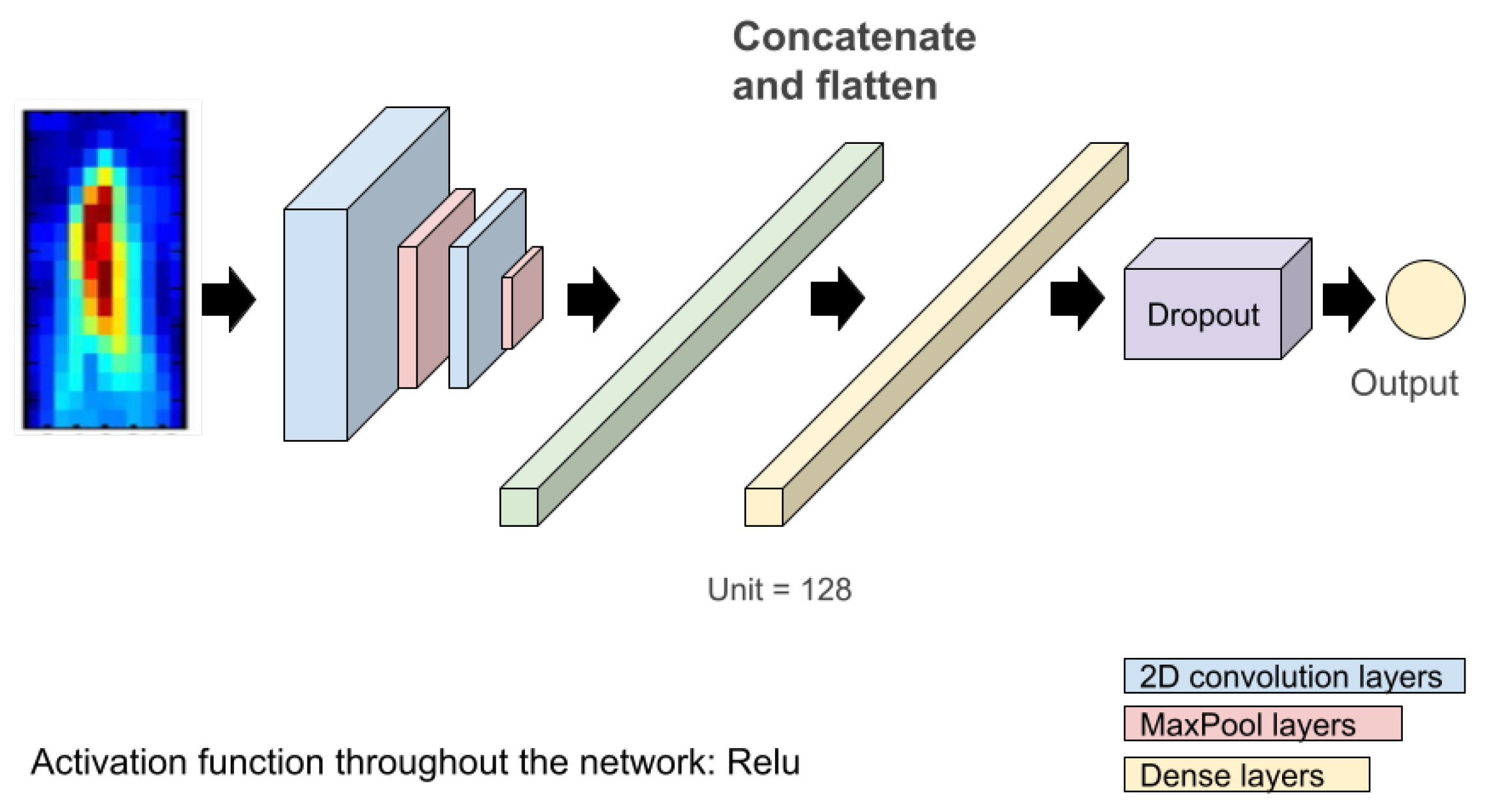
3.3. Convolutional Neural Network
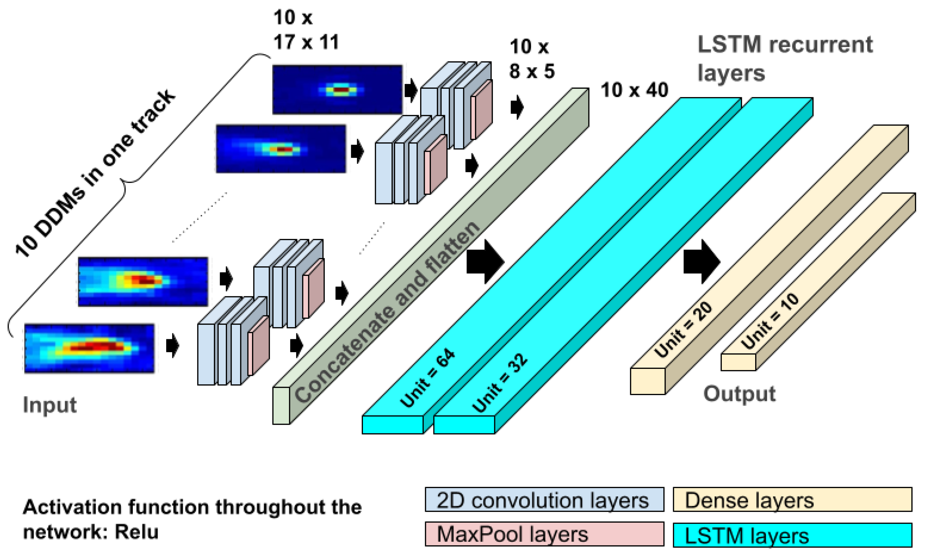
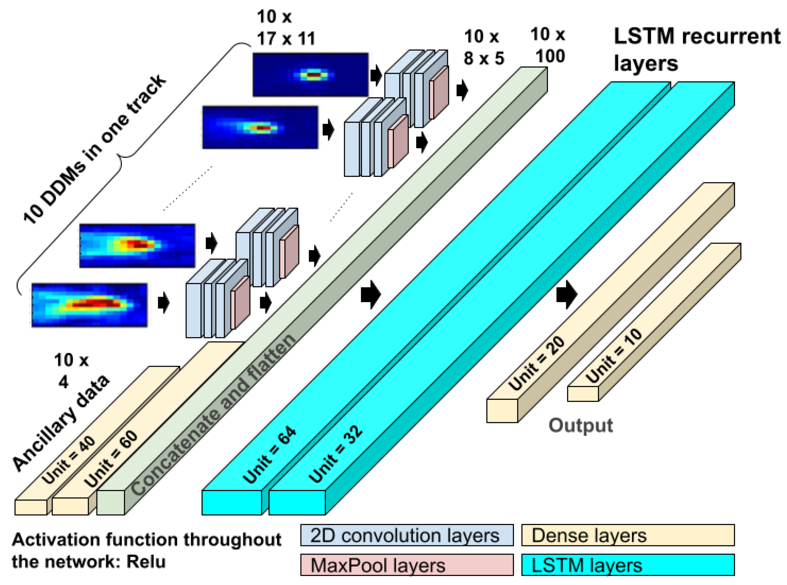
3.4. Hybrid CNN-LSTM
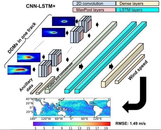
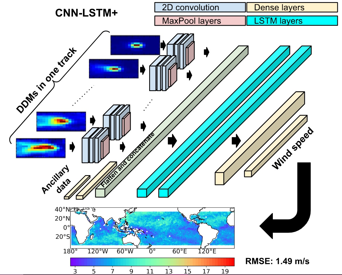
3.5. Enhanced Hybrid CNN-LSTM (CNN-LSTM+)
4. Implementation and Results
4.1. Training
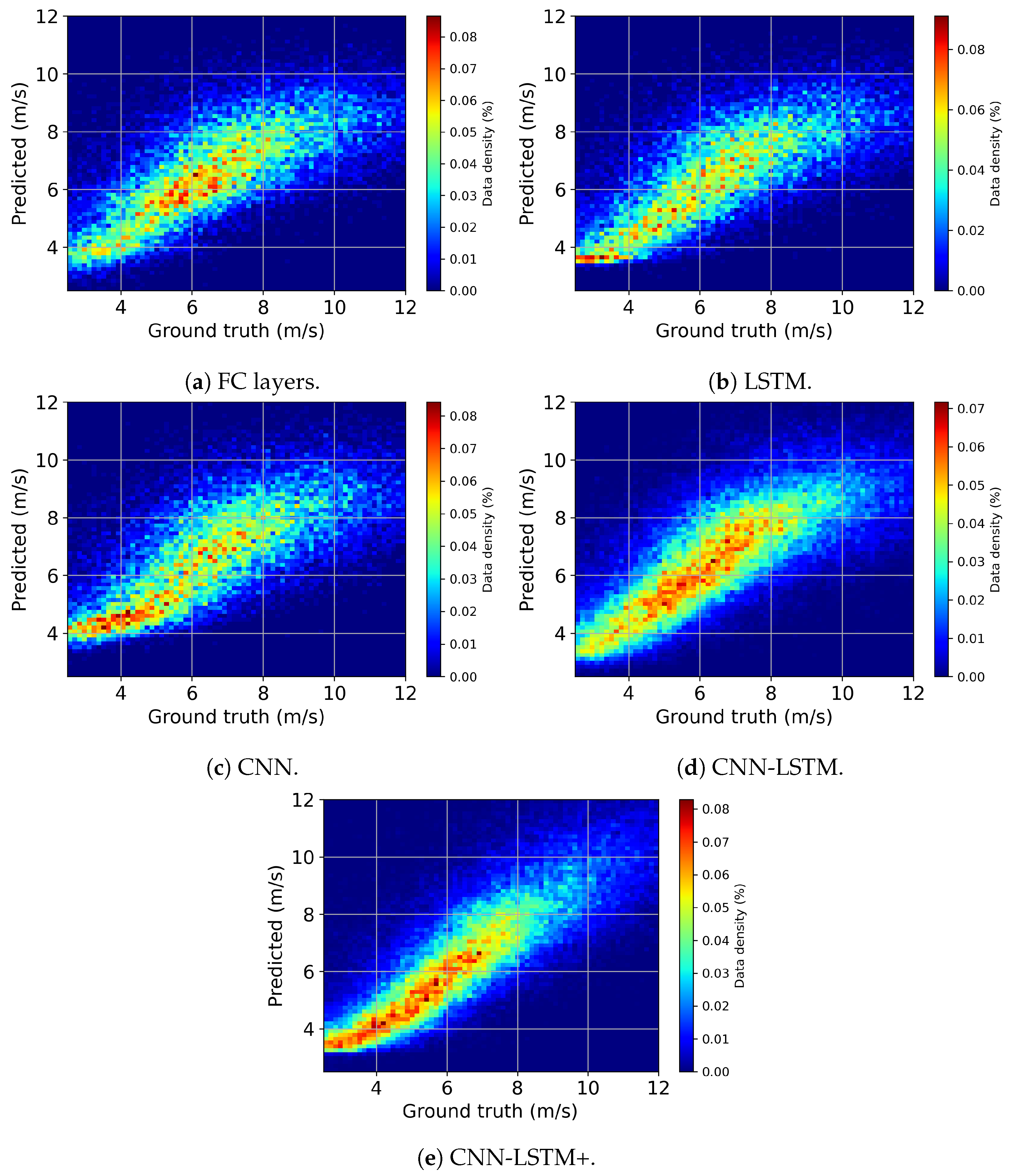
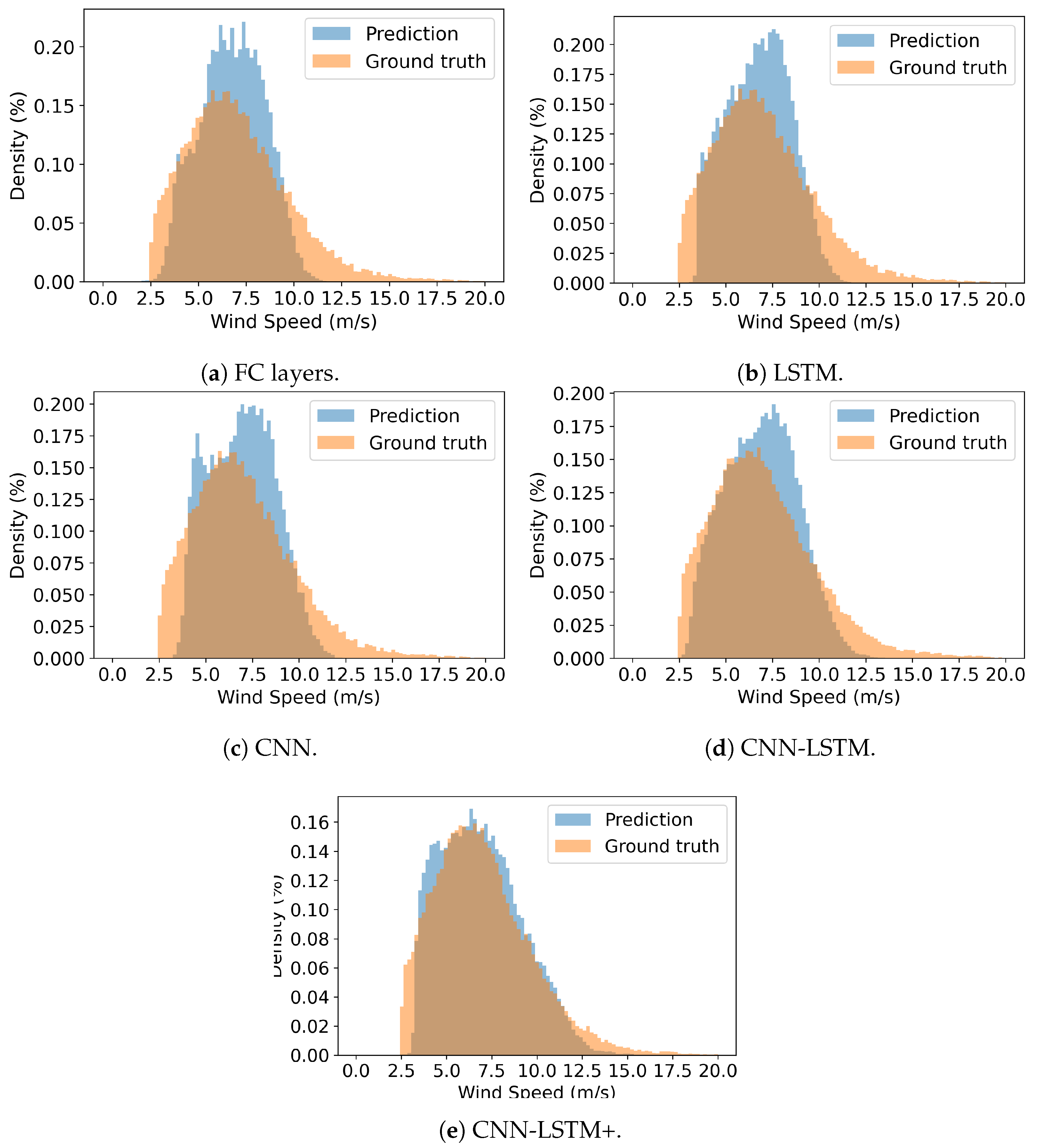
4.2. Models’ Performance
4.3. Summary and Discussion
5. Conclusions
Author Contributions
Funding
Data Availability Statement
Acknowledgments
Conflicts of Interest
References
- Woodward, A.J.; Samet, J.M. Climate change, hurricanes, and health. Am. J. Public Health 2018, 108, 33–35. [Google Scholar] [CrossRef]
- Pachauri, R.; Meyer, L.; Plattner, G.; Stocker, T. Synthesis Report. Contribution of Working Groups I, II and III to the Fifth Assessment Report of the Intergovernmental Panel on Climate Change; Intergovernmental Panel on Climate Change: Geneva, Switzerland, 2014. [Google Scholar]
- Zavorotny, V.U.; Gleason, S.; Cardellach, E.; Camps, A. Tutorial on remote sensing using GNSS bistatic radar of opportunity. IEEE Geosci. Remote Sens. Mag. 2014, 2, 8–45. [Google Scholar] [CrossRef]
- Carreno-Luengo, H.; Camps, A.; Ruf, C.; Floury, N.; Martin-Neira, M.; Wang, T.; Khalsa, S.J.; Clarizia, M.P.; Reynolds, J.; Johnson, J.; et al. The IEEE-SA working group on spaceborne GNSS-R: Scene study. IEEE Access 2021, 9, 89906–89933. [Google Scholar] [CrossRef]
- Asgarimehr, M.; Wickert, J.; Reich, S. TDS-1 GNSS reflectometry: Development and validation of forward scattering winds. IEEE J. Sel. Top. Appl. Earth Obs. Remote Sens. 2018, 11, 4534–4541. [Google Scholar] [CrossRef]
- Asgarimehr, M.; Wickert, J.; Reich, S. Evaluating impact of rain attenuation on space-borne GNSS reflectometry wind speeds. Remote Sens. 2019, 11, 1048. [Google Scholar] [CrossRef]
- Ruf, C.S.; Chew, C.; Lang, T.; Morris, M.G.; Nave, K.; Ridley, A.; Balasubramaniam, R. A new paradigm in earth environmental monitoring with the cygnss small satellite constellation. Sci. Rep. 2018, 8, 8782. [Google Scholar] [CrossRef]
- Clarizia, M.P.; Ruf, C.S.; Jales, P.; Gommenginger, C. Spaceborne GNSS-R Minimum Variance Wind Speed Estimator. IEEE Trans. Geosci. Remote Sens. 2014, 52, 6829–6843. [Google Scholar] [CrossRef]
- Garrison, J.; Komjathy, A.; Zavorotny, V.; Katzberg, S. Wind speed measurement using forward scattered GPS signals. IEEE Trans. Geosci. Remote Sens. 2002, 40, 50–65. [Google Scholar] [CrossRef]
- Li, C.; Huang, W. An Algorithm for Sea-Surface Wind Field Retrieval From GNSS-R Delay-Doppler Map. IEEE Geosci. Remote Sens. Lett. 2014, 11, 2110–2114. [Google Scholar] [CrossRef]
- Asgarimehr, M.; Zhelavskaya, I.; Foti, G.; Reich, S.; Wickert, J. A GNSS-R geophysical model function: Machine learning for wind speed retrievals. IEEE Geosci. Remote Sens. Lett. 2019, 17, 1333–1337. [Google Scholar] [CrossRef]
- Reynolds, J.; Clarizia, M.P.; Santi, E. Wind speed estimation from CYGNSS using artificial neural networks. IEEE J. Sel. Top. Appl. Earth Obs. Remote Sens. 2020, 13, 708–716. [Google Scholar] [CrossRef]
- Asgarimehr, M.; Arnold, C.; Weigel, T.; Ruf, C.; Wickert, J. GNSS reflectometry global ocean wind speed using deep learning: Development and assessment of CyGNSSnet. Remote Sens. Environ. 2022, 269, 112801. [Google Scholar] [CrossRef]
- Guo, W.; Du, H.; Guo, C.; Southwell, B.J.; Cheong, J.W.; Dempster, A.G. Information fusion for GNSS-R wind speed retrieval using statistically modified convolutional neural network. Remote Sens. Environ. 2022, 272, 112934. [Google Scholar] [CrossRef]
- Zhao, D.; Heidler, K.; Asgarimehr, M.; Arnold, C.; Xiao, T.; Wickert, J.; Zhu, X.X.; Mou, L. DDM-Former: Transformer networks for GNSS reflectometry global ocean wind speed estimation. Remote Sens. Environ. 2023, 294, 113629. [Google Scholar] [CrossRef]
- Saïd, F.; Jelenak, Z.; Park, J.; Chang, P.S. The NOAA track-wise wind retrieval algorithm and product assessment for CyGNSS. IEEE Trans. Geosci. Remote Sens. 2021, 60, 1–24. [Google Scholar] [CrossRef]
- Lu, C.; Wang, Z.; Wu, Z.; Zheng, Y.; Liu, Y. Global ocean wind speed retrieval from GNSS reflectometry using CNN-LSTM network. IEEE Trans. Geosci. Remote Sens. 2023, 61, 5801112. [Google Scholar] [CrossRef]
- Hersbach, H.; Bell, B.; Berrisford, P.; Hirahara, S.; Horányi, A.; Muñoz-Sabater, J.; Nicolas, J.; Peubey, C.; Radu, R.; Schepers, D.; et al. The ERA5 global reanalysis. Q. J. R. Meteorol. Soc. 2020, 146, 1999–2049. [Google Scholar] [CrossRef]
- Williams, R.J.; Zipser, D. A learning algorithm for continually running fully recurrent neural networks. Neural Comput. 1989, 1, 270–280. [Google Scholar] [CrossRef]
- Srivastava, N.; Hinton, G.; Krizhevsky, A.; Sutskever, I.; Salakhutdinov, R. Dropout: A Simple Way to Prevent Neural Networks from Overfitting. J. Mach. Learn. Res. 2014, 15, 1929–1958. [Google Scholar]
- Pascanu, R.; Mikolov, T.; Bengio, Y. On the difficulty of training recurrent neural networks. In Proceedings of the International Conference on Machine Learning, Atlanta, GA, USA, 17–19 June 2013; pp. 1310–1318. [Google Scholar]
- Schmidhuber, J.; Hochreiter, S. Long short-term memory. Neural Comput. 1997, 9, 1735–1780. [Google Scholar]
- Graves, A. Generating sequences with recurrent neural networks. arXiv 2013, arXiv:1308.0850. [Google Scholar]
- Yu, Y.; Si, X.; Hu, C.; Zhang, J. A review of recurrent neural networks: LSTM cells and network architectures. Neural Comput. 2019, 31, 1235–1270. [Google Scholar] [CrossRef] [PubMed]
- Sherstinsky, A. Fundamentals of recurrent neural network (RNN) and long short-term memory (LSTM) network. Phys. D Nonlinear Phenom. 2020, 404, 132306. [Google Scholar] [CrossRef]
- Gope, P.; Sarkar, S.; Mitra, P. Prediction of extreme rainfall using hybrid convolutional-long short term memory networks. In Proceedings of the 6th International Workshop on Climate Informatics: CI, Boulder, CO, USA, 21–23 September 2016; Volume 2016. [Google Scholar]
- Xingjian, S.; Chen, Z.; Wang, H.; Yeung, D.Y.; Wong, W.K.; Woo, W.c. Convolutional LSTM network: A machine learning approach for precipitation nowcasting. In Proceedings of the Advances in Neural Information Processing Systems, Montreal, QC, Canada, 7–12 December 2015; pp. 802–810. [Google Scholar] [CrossRef]
- Tianyu, Z.; Zhenjiang, M.; Jianhu, Z. Combining cnn with hand-crafted features for image classification. In Proceedings of the 2018 14th IEEE International Conference on Signal Processing (ICSP), Beijing, China, 12–16 August 2018; pp. 554–557. [Google Scholar] [CrossRef]
- Kingma, D.P.; Ba, J. Adam: A method for stochastic optimization. arXiv 2014, arXiv:1412.6980. [Google Scholar]
- Asgarimehr, M.; Zavorotny, V.; Wickert, J.; Reich, S. Can GNSS reflectometry detect precipitation over oceans? Geophys. Res. Lett. 2018, 45, 12–585. [Google Scholar] [CrossRef]
- Ruf, C.S.; Gleason, S.; McKague, D.S. Assessment of CYGNSS wind speed retrieval uncertainty. IEEE J. Sel. Top. Appl. Earth Obs. Remote Sens. 2018, 12, 87–97. [Google Scholar] [CrossRef]
- Ruf, C.S.; Balasubramaniam, R. Development of the CYGNSS geophysical model function for wind speed. IEEE J. Sel. Top. Appl. Earth Obs. Remote Sens. 2018, 12, 66–77. [Google Scholar] [CrossRef]
- Clarizia, M.P.; Zavorotny, V.; Ruf, C. CYGNSS algorithm theoretical basis document level 2 wind speed retrieval. Revision 2015, 2, 148-0138. [Google Scholar]


| Architecture | RMSE (m/s) | Bias (m/s) | Training Epochs | Training MSE (m/s) | Validation MSE (m/s) |
|---|---|---|---|---|---|
| FC layers | 1.93 | −0.24 | 40 | 3.89 | 3.79 |
| LSTM | 1.92 | −0.28 | 87 | 3.77 | 3.75 |
| CNN | 1.92 | −0.08 | 94 | 3.86 | 3.78 |
| CNN-LSTM | 1.84 | −0.12 | 54 | 3.03 | 3.29 |
| CNN-LSTM+ | 1.49 | −0.08 | 50 | 2.22 | 2.26 |
| MVE | 1.90 | 0.20 | - | - | - |
Disclaimer/Publisher’s Note: The statements, opinions and data contained in all publications are solely those of the individual author(s) and contributor(s) and not of MDPI and/or the editor(s). MDPI and/or the editor(s) disclaim responsibility for any injury to people or property resulting from any ideas, methods, instructions or products referred to in the content. |
© 2023 by the authors. Licensee MDPI, Basel, Switzerland. This article is an open access article distributed under the terms and conditions of the Creative Commons Attribution (CC BY) license (https://creativecommons.org/licenses/by/4.0/).
Share and Cite
Arabi, S.; Asgarimehr, M.; Kada, M.; Wickert, J. Hybrid CNN-LSTM Deep Learning for Track-Wise GNSS-R Ocean Wind Speed Retrieval. Remote Sens. 2023, 15, 4169. https://doi.org/10.3390/rs15174169
Arabi S, Asgarimehr M, Kada M, Wickert J. Hybrid CNN-LSTM Deep Learning for Track-Wise GNSS-R Ocean Wind Speed Retrieval. Remote Sensing. 2023; 15(17):4169. https://doi.org/10.3390/rs15174169
Chicago/Turabian StyleArabi, Sima, Milad Asgarimehr, Martin Kada, and Jens Wickert. 2023. "Hybrid CNN-LSTM Deep Learning for Track-Wise GNSS-R Ocean Wind Speed Retrieval" Remote Sensing 15, no. 17: 4169. https://doi.org/10.3390/rs15174169
APA StyleArabi, S., Asgarimehr, M., Kada, M., & Wickert, J. (2023). Hybrid CNN-LSTM Deep Learning for Track-Wise GNSS-R Ocean Wind Speed Retrieval. Remote Sensing, 15(17), 4169. https://doi.org/10.3390/rs15174169