Article

Use of High-Resolution Land Cover Maps to Support the Maintenance of the NWI Geospatial Dataset: A Case Study in a Coastal New Orleans Region

1
Department of Geographical Sciences, University of Maryland, College Park, MD 20742, USA
2
U.S. Fish and Wildlife Service, National Wetlands Inventory, Falls Church, VA 22041, USA
3
Department of Environmental Science & Technology, University of Maryland, College Park, MD 20742, USA
4
U.S. Department of Agriculture, Agricultural Research Service, Beltsville, MD 20705, USA
5
U.S. Fish and Wildlife Service, National Wetlands Inventory, Madison, WI 53711, USA
6
U.S. National Oceanic and Atmospheric Administration, North Charleston, SC 29405, USA
*
Author to whom correspondence should be addressed.
Remote Sens. 2023, 15(16), 4075; https://doi.org/10.3390/rs15164075
Submission received: 9 July 2023 / Revised: 15 August 2023 / Accepted: 16 August 2023 / Published: 18 August 2023

Abstract

:
The National Wetlands Inventory (NWI) is the most comprehensive wetland geospatial dataset in the United States. However, it can be time-consuming and costly to maintain. This study introduces automated algorithms and methods to support NWI maintenance. Through a wall-to-wall comparison between NWI and Coastal Change Analysis Program (C-CAP) datasets, a pixel-level difference product was generated at 1 m resolution. Building upon this, supplementary attributes describing wetland changes were incorporated into each NWI polygon. Additionally, new water polygons were extracted from C-CAP data, and regional statistics regarding wetland changes were computed for HUC12 watersheds. The 1 m difference product can indicate specific wetland change locations, such as wetland loss to impervious surfaces, the gain of open water bodies from uplands, and the conversion of drier vegetated wetlands to open water. The supplementary attributes can indicate the amount and percentage of wetland loss or water regime change for NWI polygons. Extracted new water polygons can serve as preliminary materials for generating NWI standard-compliant products, expediating NWI maintenance processes while reducing costs. Regional statistics of wetland change can help target watersheds with the most significant changes for maintenance, thereby reducing work areas. The approaches we present hold significant value in supporting NWI maintenance.

Graphical Abstract

1. Introduction

Wetlands are among the most important ecosystems, providing habitat for a wide variety of plant and animal species [1]. Wetlands across the globe have undergone substantial losses [2]. Wetland degradation and loss are occurring at a greater rate compared to other ecosystem types [3]. These changes are caused by natural drivers [4], such as sea level rise [5], droughts [6], and climate change [7], as well as anthropogenic drivers [4], such as land-use change [8], dam construction [9], and population growth [10]. The U.S. Fish and Wildlife Service National Wetland Inventory (NWI) is the most comprehensive wetland geospatial dataset for the U.S. [11]. However, a significant portion of the NWI geospatial dataset is outdated [11]. Wetlands across the United States have changed substantially since the NWI Program first started mapping wetlands in the 1970s. During this time period, some wetlands have been lost, while others have been created [12]. Additionally, the geometry of some NWI polygons created decades ago have lower accuracy, which can lead to geospatial mismatches between the old NWI polygons and current high-resolution geospatial datasets.
Accurate and contemporary wetland geospatial datasets are indispensable to stakeholders in decision making regarding wetland conservation, wildlife habitat protection, and sustainable land use and land cover management [13]. There is a need to bring the NWI dataset up to date. Generating standard-compliant NWI products, following the requirements of the Federal Geographic Data Committee [14], involves acquiring high-resolution images, conducting field surveys, collecting ancillary data, manually delineating most wetland polygons, and classification of wetland type by experts. Although more accurate than fully automated processes, this mainly manual workflow is time-consuming and costly. Updating the entire NWI dataset using this approach likely take several years. By the time the processes are finished, new wetland changes may have already occurred.
Early wetland mapping and change studies relied heavily on field surveys [15,16]. In an examination of 233 Oregon NWI features mapped in 1981, field surveys uncovered that, within a decade, 40% of them had succumbed to destruction due to human activities, primarily through conversion to urban and agricultural land uses [15]. Field surveys can collect the most accurate wetland status and change information, which is valuable for wetland updates and maintenance. However, due to their labor-intensive, costly, and time-consuming nature, field surveys often cover only limited areas. To overcome these challenges, during the initial stages, moderate-resolution satellite imagery, such as 30 m Landsat data and 20 m SPOT-XS data, emerged as a solution for detecting wetland changes across large regions [17]. Various methodologies were employed, including image differencing [18], outlier pixel detection [19], and rule-based classification [17]. For instance, logical rules were developed by combining SPOT-XS pixel mean modulus value, majority land-cover value, and NWI wetland class, enabling the classification of wetland polygons into ‘changed’ and ‘not-changed’ categories. Although moderate-resolution satellite imagery serves well in regional-scale wetland monitoring, it falls short for the kind of detailed, parcel-scale wetland mapping and classification that is performed by the NWI Program [19]. This inadequacy arises because modern NWI wetland features are established based on high-resolution aerial photos at meter or submeter scales.
Recent wetland studies leveraged high-solution remote sensing data, including lidar point cloud data [20], radar images [21], aerial photos [22], and topographic data [23]. These studies have harnessed computation-intensive methods, such as machine learning algorithms [22,24] and deep learning models [20,23], which offer greater efficiency compared to traditional approaches like aerial image interpretation and field surveys [21]. However, these automated wetland mapping approaches have not proved capable of producing FGDC standard-compliant wetland data, perhaps in part due to differing research objectives [25]. These experimental studies use distinct wetland classification systems, input materials, and operational procedures, resulting in wetland maps that may exhibit discrepancies of up to 50% when compared to NWI [11]. Consequently, it is challenging to use these maps to update NWI datasets.
Although it does not meet FGDC Wetland Mapping Standards, The National Oceanic and Atmospheric Administration (NOAA) Coastal Change Analysis Program (C-CAP) 1 m land cover map employs a wetland classification compatible with NWI and is projected to cover the entire coastal region of the CONUS in a couple of years [26], making it an excellent candidate for detecting wetland changes and supporting NWI maintenance. This study develops an automatic approach for creating difference products to support the maintenance of the NWI geospatial dataset using 1 m C-CAP land cover maps. The goal is to speed up the maintenance process and reduce costs. Since the generation of compliant NWI products requires a lot of field sampling data, such as vegetation type, water regime, and substrate information [14], the entire process cannot be automated. Given these constraints, our objectives for automated maintenance include identifying regions with the greatest need for updates and improving the efficiency of updating NWI data in those regions. In particular, some of the changes that can be easily identified are wetland loss to impervious surfaces, the gain of open water from uplands, and the conversion of drier vegetated wetlands to open surface water.
Wetland change is an ongoing phenomenon across the U.S., particularly in rapidly developing suburban regions. It is urgent to update and maintain the NWI dataset. However, as previously noted, field survey methods are costly and time-consuming, wetland products derived from moderate-resolution satellite imagery lack the precision needed for NWI updates, and recent machine learning techniques often do not adhere to NWI wetland protocols, rendering their resultant maps unsuitable for NWI maintenance. This study seeks to address these gaps by developing cost-efficient and automated approaches to update and maintain the NWI dataset, utilizing 1 m C-CAP data. The objectives of this study are fourfold: (1) to generate pixel-level difference products at a 1 m resolution to pinpoint wetland change locations; (2) to calculate new attributes that describe wetland changes for NWI polygons; (3) to extract new water polygons from C-CAP data to expediate NWI maintenance process; and (4) to compute regional statistics on wetland changes, aiming to identify HUC12 watersheds with the most urgent maintenance needs.

2. Materials and Methods

2.1. Study Area

Our study was conducted around New Orleans, Louisiana, as shown in Figure 1a. The study region covers approximately 20,500 km2. The study area includes the Mississippi River Delta, New Orleans, and the Tangipahoa River basin, as indicated in Figure 1c. Wetlands in these regions have important roles in protecting local communities from hurricane storm surges and flooding [27]. However, wetlands in these regions are being modified due to threats from development, sea level rise, subsidence, etc. Wetlands in the Mississippi River Delta area have been affected by sea level rise [28] and the sediment load discharge of the Mississippi River [29]. Wetlands in the New Orleans–Metairie metropolitan region face pressure from urbanization [30]. In addition, the mining of sand and gravel in floodplains of the Tangipahoa River has caused erosion and deposition, resulting in changes in the rivers’ flow and shape [31]. The study area is one of the few regions across the U.S. that currently have 1 m resolution C-CAP land cover maps. Furthermore, the abundance of wetlands and various wetland types in this region makes it an ideal place to carry out our research.

2.2. Data

2.2.1. NWI

The U.S. Fish and Wildlife Service established the NWI Program, which includes polygons of wetlands and deep-water habitats in its geospatial dataset. Trained image analysts manually delineated these polygons from aerial and fine resolution satellite imagery. Wetland experts then determined the attributes of these polygons, such as information about the wetland substrate type, vegetation type, water regime type, and water chemistry type, based on their assessments of field sampling data and the Cowardin wetland classification system [14,32]. The NWI dataset for the study area was obtained from the U.S. Fish and Wildlife Service Wetlands Mapper in July 2021 [33]. There were approximately 146,000 NWI wetland polygons within the study area. These wetland polygons were created by 84 projects spanning several decades: 17 projects from the 1970s, 56 from the 1980s, 1 from the 1990s, 3 from the 2000s, 6 from 2010 to 2016, and 1 from 2017 (Figure 1b). The NWI project from 2017 was excluded from further analysis because it was created in the same year as the C-CAP data.

2.2.2. C-CAP 1 m Dataset

The C-CAP 1 m land cover data used in this study were generated by the NOAA Coastal Change Analysis Program [26]. The dataset includes 18 land cover categories, such as impervious surface, open surface water, wetland, etc. (Figure 1c). The impervious surface layer was derived from 15 to 30 cm imagery around 2017. The water layer was derived using feature recognition classification technology with manual refinement. Wetlands were classified through a modeling process that made use of NWI, soil data, topographic derivatives, etc. [26]. The C-CAP data were obtained from the NOAA Office for Coastal Management in January 2022 [26]. According to its accuracy assessment, the overall accuracy of this product is 93.5% for all land cover categories.

2.2.3. Time Series Inundation Data

The Dynamic Surface Water Extent (DSWE) algorithms were developed to generate water inundation products [34,35]. The DSWE algorithms employ several water classification methods to detect water. A pixel with a higher number of water detections from these methods indicates a higher probability of this pixel being water. These pixels were then divided into five categories: water of high confidence, water of moderate confidence, partial water/potential wetland, low confidence water or wetland, and dry land [34]. We translated the DSWE algorithms into JavaScript. All clear Landsat images captured during 2016–2018 were used to create a time series of DSWE inundation frequency at 30 m spatial resolution in the cloud computing platform of Google Earth Engine (GEE) [36]. Subsequently, these time series inundation datasets were downloaded from GEE to local high-performance computers for further analysis.

2.3. Methods

The methodological approach used in this study is illustrated in Figure 2 and comprises four main stages of analysis: (1) difference analysis between old NWI data and recent C-CAP map through a wall-to-wall comparison at a 1 m scale; (2) wetland loss analysis for all wetland polygons and water regime change analysis for drier vegetated wetland polygons; (3) water body extraction from the 1 m C-CAP map and classification of new water bodies based on their distance from the original NWI polygons; and (4) generation of statistics for wetland changes at HUC12 watersheds.

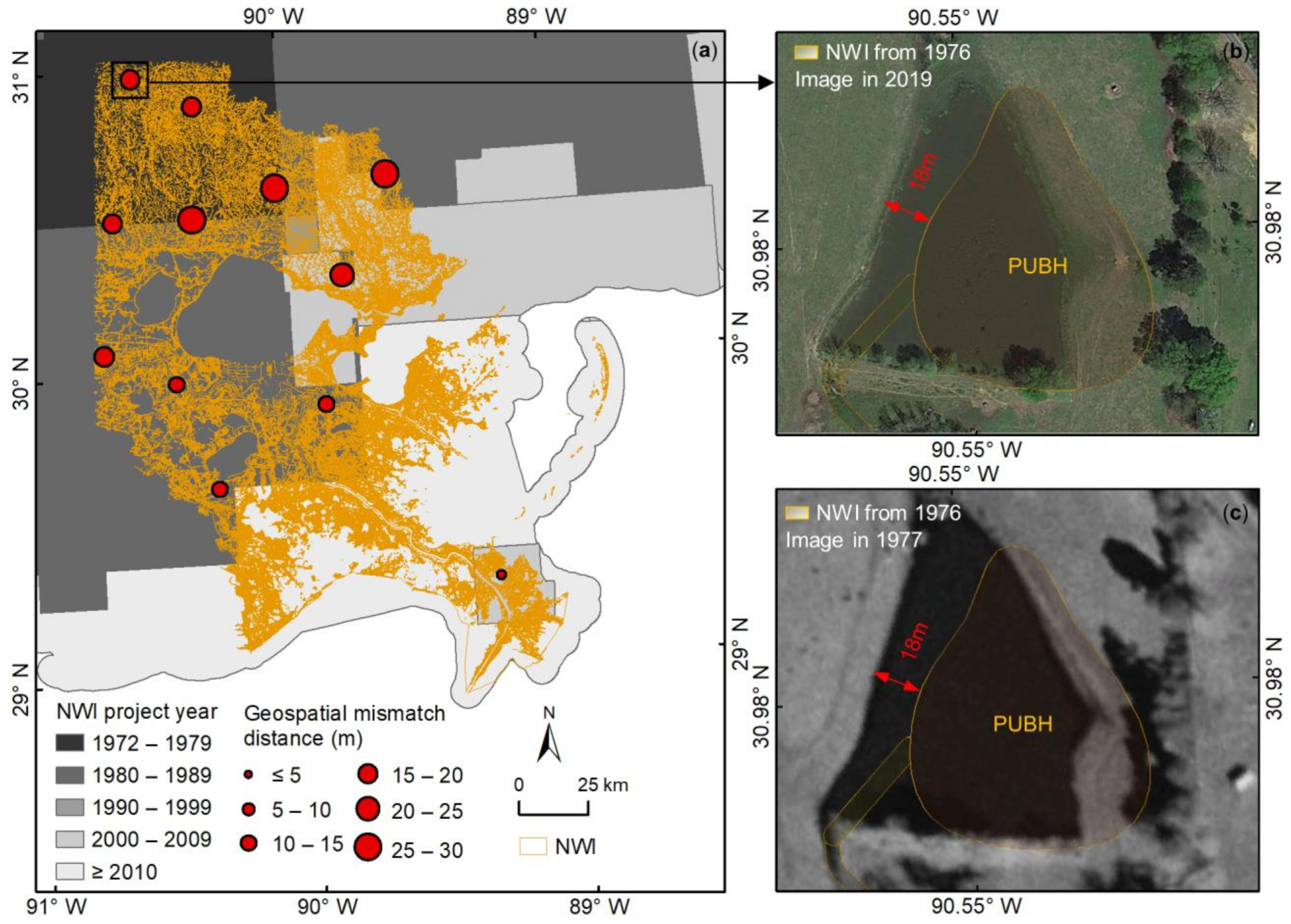
2.3.1. Derivation and Validation of the Pixel Level Difference Product

We focused on wetland changes that can be easily detected and reliably mapped by remote sensing images and land cover products. The impervious surface and open surface water have very high mapping accuracy, approximately 98% and 100%, respectively [26]. This study detected wetland changes by carrying out a wall-to-wall comparison between the NWI geospatial dataset and the impervious surface and water layers from the C-CAP dataset (Figure 2). Specifically, we focused on three aspects: NWI wetland to C-CAP impervious surface, NWI Upland to C-CAP open water, and NWI drier vegetated wetland to C-CAP open water. We did not consider changes in wetland types between NWI and C-CAP, such as emergent wetland to scrub/shrub wetland. This is because these wetland ecosystems continue to provide important services, and it is challenging to verify these changes using remote sensing images.
It should be noted that some NWI wetland and deep-water features, such as coastline waters, submerged lagoons and estuaries, and large deep-water lakes (>8 ha in area, >2.5 m in depth), are not expected to experience significant changes and have therefore been excluded from the wetland loss assessment. Riverine features are a common type of wetland in the NWI database. However, their elongated polygonal shape increases the likelihood of geospatial mismatch between the NWI and the C-CAP datasets. Additionally, river networks are well protected by law. As a result, all riverine features have been excluded from the assessment of wetland loss. Approximately 130,000 NWI features within the study area were included for analysis.
To speed up the data processing and apply parallel computing methods, the C-CAP 1 m dataset of the study area was subset into 187 HUC12 watersheds (Figure 2). Next, the NWI polygons within each HUC12 watershed were selected from the entire NWI geospatial dataset. These polygons were then converted into a 1 m raster format. Subsequently, the NWI pixels and C-CAP pixels were compared at the 1 m scale to identify any differences between them. Finally, the difference products for each HUC12 watershed were merged to create a single mosaic that provides an overview of the discrepancies between the two datasets.
The validation of different products focused on three categories: wetland to impervious surface, upland to open water, and drier vegetated wetland to open water. We used a stratified random sampling technique to select samples for validation. For each category, we randomly selected 200 samples. Additionally, for the referencing categories of wetland not changed to impervious surface, upland not changed to open water, and drier vegetated wetland not changed to open water, we also randomly selected 200 samples for each category. In total, 1200 random samples were selected and loaded into Google Earth. A high-resolution image in Google Earth from around 2017 was chosen as the reference to validate each sample.
When we examined the difference products, we observed geospatial mismatches between the old NWI geospatial dataset and recent high-resolution data. The earlier NWI projects were created on a smaller scale (1:250,000), using relatively coarser-resolution images compared to later projects (1:24,000). As a result, some of the NWI polygons created several decades ago may contain geospatial inaccuracies. We measured geospatial shifting through a few samples taken across the study area.

2.3.2. Calculation of New Attributes for NWI Wetland Polygons

We overlaid the boundary of each NWI polygon on top of the difference products to calculate the amount of wetland loss. Two new attributes were added to each NWI polygon: the area of wetland loss within an NWI polygon and the percentage of this NWI polygon that was converted to an impervious surface. Wetlands that have been converted to impervious surfaces are difficult to restore and are considered permanent losses [37]. Therefore, by using the two attributes mentioned above, we can identify NWI polygons with the most significant permanent wetland loss, especially those with near 100% permanent loss.
The drier vegetated NWI polygons are wetland areas dominated by vegetation such as emergent, scrub-shrub, and forest. They are characterized by relatively drier water regimes. The list of all possible attributes of drier vegetated wetlands was acquired from Fish and Wildlife Service NWI experts who generated the NWI dataset. Each NWI polygon in the study area was compared to the list of drier vegetated wetland attributes to determine whether it was a drier vegetated wetland polygon. The water regimes of NWI polygons are listed in Table 1. Drier vegetated wetland polygons have water regimes that include temporarily flooded (A), seasonally saturated (B), seasonally flooded (C), regularly flooded (N), irregularly flooded (P), seasonally flooded–fresh tidal (R), and temporarily flooded–fresh (S).
Within the study area, there were approximately 100,000 NWI polygons that had vegetation and drier water regimes, and were thus classified as drier vegetated wetlands. For each drier vegetated wetland polygon, we calculated the statistics of open surface water based on the difference products. Two new attributes were then added to each drier vegetated polygon: the area of open water within the drier vegetated wetland polygon and the percentage of the polygon that had been converted to open water. The water layer in the C-CAP dataset was based on single-temporal images rather than time series images, meaning that some of the water bodies captured by the C-CAP dataset could be temporary water.
To avoid the impacts of such temporary water, we calculated and added the average DSWE inundation frequency attribute to each drier vegetated wetland polygon. Considering possible impacts of geospatial mismatches between the old NWI polygons and the 30 m DSWE inundation frequency dataset, we shrank the NWI polygons by 30 m before calculating the average DSWE inundation frequency attribute. In this way, only the larger NWI polygons with at least one pixel of DSWE inundation frequency data could have the attribute of DSWE inundation information. Smaller NWI polygons will not have DSWE inundation information. Therefore, if the average DSWE inundation frequency attribute is available, the drier vegetated wetland polygons with permanent water coverage in C-CAP should also have high average DSWE inundation frequency values.
The new attributes mentioned above enable us to quantify the extent of changes that have occurred in NWI polygons, allowing for a more focused analysis of the wetland polygons that have experienced the most significant changes.

2.3.3. Delineation of New Water Body Polygons

New water body polygons were derived from the C-CAP 1 m dataset. First, the land cover maps were converted into a water/non-water map. Small water objects or holes with an area of 5 pixels or fewer were then filtered out to remove any noise or irrelevant features. Next, large water objects, including coastline waters, with a continuous area greater than 100 km2 were masked out since they were outside the scope of this study. The raster was then converted into polygons to create distinct and easily recognizable features. The geospatial mismatch between old NWI polygons and recent high-resolution images has made the classification of new water bodies more difficult. For example, a water body from the C-CAP map may not be a new water body if it is close to or overlapping with old NWI polygons. This is simply because the old NWI polygons could have undergone geospatial shifting. Thus, we classified the derived water polygons into three categories based on their distance from the original NWI polygons. The categories were polygons overlapping with the original NWI polygons, polygons within a 30 m distance of the original NWI polygons, and polygons located at least 30 m away from the original NWI polygons. Finally, the water polygons were smoothed using ArcMap software with the PEAK algorithm. We also calculated and added the average DSWE inundation frequency attribute to water polygons derived from the C-CAP dataset. This attribute could be used to remove temporal inundation while keeping the permanent water bodies.

2.3.4. Calculation of Difference Statistics at the Watershed Scale

We calculated the statistics of total wetland change for HUC12 watersheds, including the total area of wetland loss to impervious surface, upland to open water, and drier vegetated wetland to open water. The size of the watershed affects the total area of wetland change, so we normalized the area of wetland change by the area of the watersheds. This gives us the area of wetland change per unit of watershed area, allowing for a comparison across different watersheds. The total area of wetland change and normalized area of wetland change are both useful in identifying regions that have experienced the most significant wetland changes.

3. Results

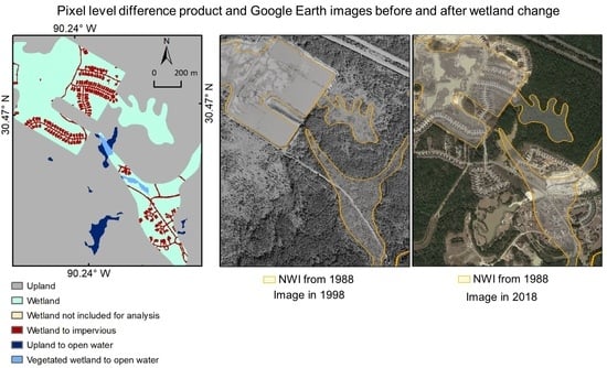
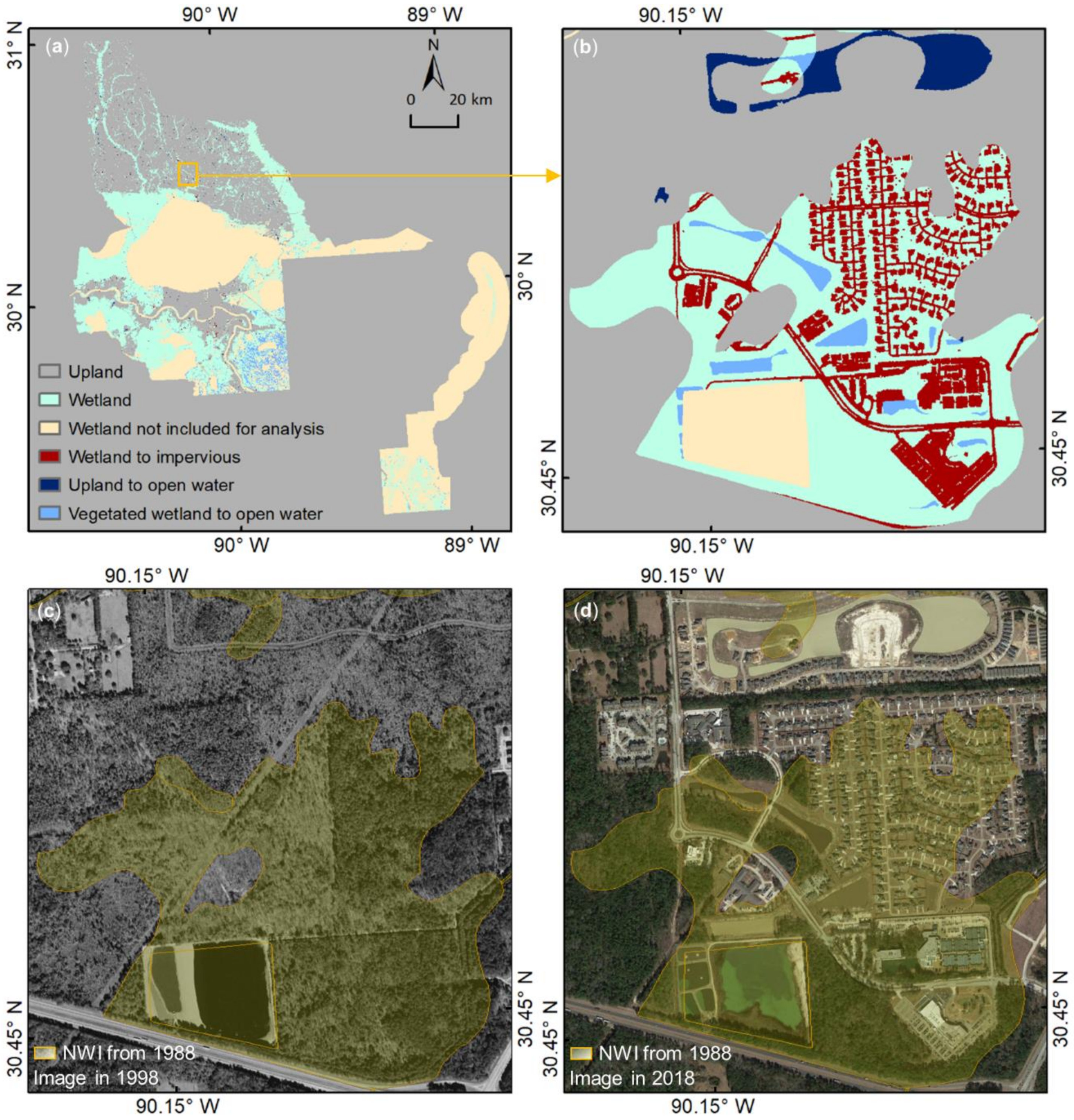
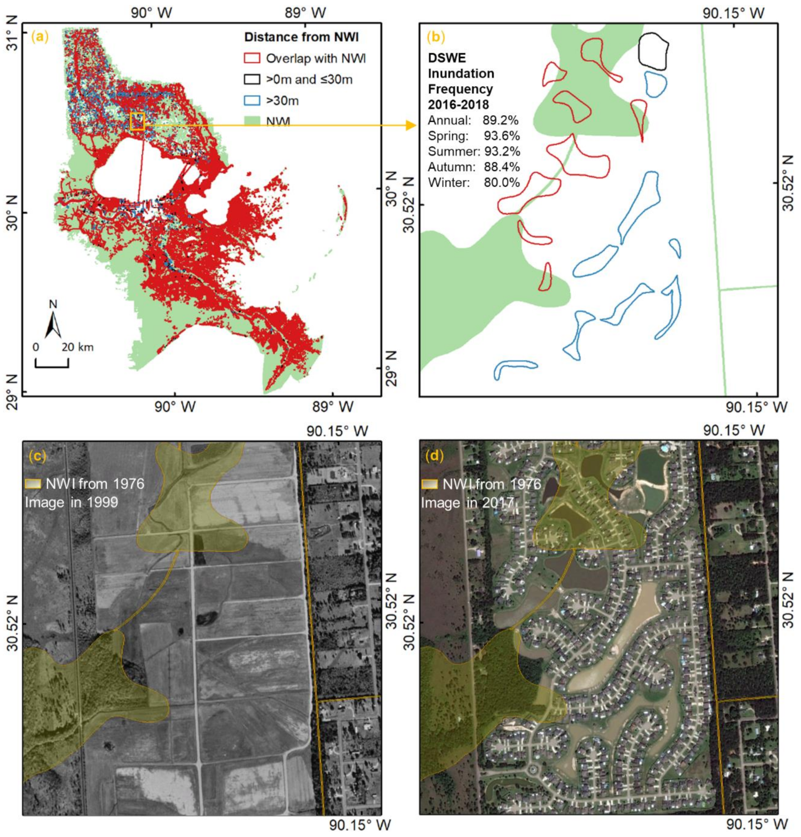
3.1. Pixel Level Differences and Wetland Change

The pixel level difference product identified three classes that likely indicated wetland changes, including wetland to impervious surface, upland to open water, and vegetated wetland to open water. As discussed in Section 2.3.1, deep-water and riverine wetlands were not analyzed in this study. Figure 3 shows the difference product and a zoomed-in example together with high resolution digital aerial photos acquired in 1998 and 2017 over the zoomed-in area. The NWI polygon in the zoomed-in window was a forested wetland with water regime A (temporarily flooded). A large part of this wetland was converted to a developed suburban area consisting of buildings, roads, storm water ponds/lakes, and other urban fabrics. The difference product at 1 m resolution shows the specific locations where wetlands have been converted to urban impervious surfaces or ponds, as well as where uplands have been converted to open water.
Based on the 1200 validation points selected using stratified random sampling methods, the overall accuracies of the wetland loss to impervious surface, upland to open water, and drier vegetated wetland to open water area are 0.96, 0.99, and 0.94, respectively. Of the 200 samples mapped as wetland loss to impervious surfaces, 185 had real changes according to available high-resolution images (Table 2). For the upland to open water change class, 197 out of 200 validation samples had real changes (Table 3), and for the drier vegetated wetland to open water change class, 189 out of 200 samples had real changes (Table 4).
By checking the NWI polygons against recent and historical high-resolution images in Google Earth, we found that geospatial mismatches only occur sporadically and are not systematic. They were randomly distributed across the study region. We measured geospatial mismatch distances at 12 random locations within the study area. Based on these limited measurements, geospatial mismatches range from a few meters to as large as 30 m in this region. However, in other regions, geospatial mismatches as large as 50 m have been observed. Additionally, we observed that older NWI polygons tend to have relatively larger geospatial mismatch distances, as shown in Figure 4.
The study area has experienced a total wetland loss of 18.97 km2 to impervious surfaces, a total gain of 31.81 km2 of open water from uplands, and a total change of 232.54 km2 from drier vegetated wetland to open water. The area of drier vegetated wetland converted to open water is much larger than the areas of wetland converted to impervious surface and upland converted to open water. The study area encompasses a large coastal region, and the significant conversion of drier vegetated wetland to open water in this area may be attributed to sea level rise and the decline of sediment in the Mississippi River Delta [29].

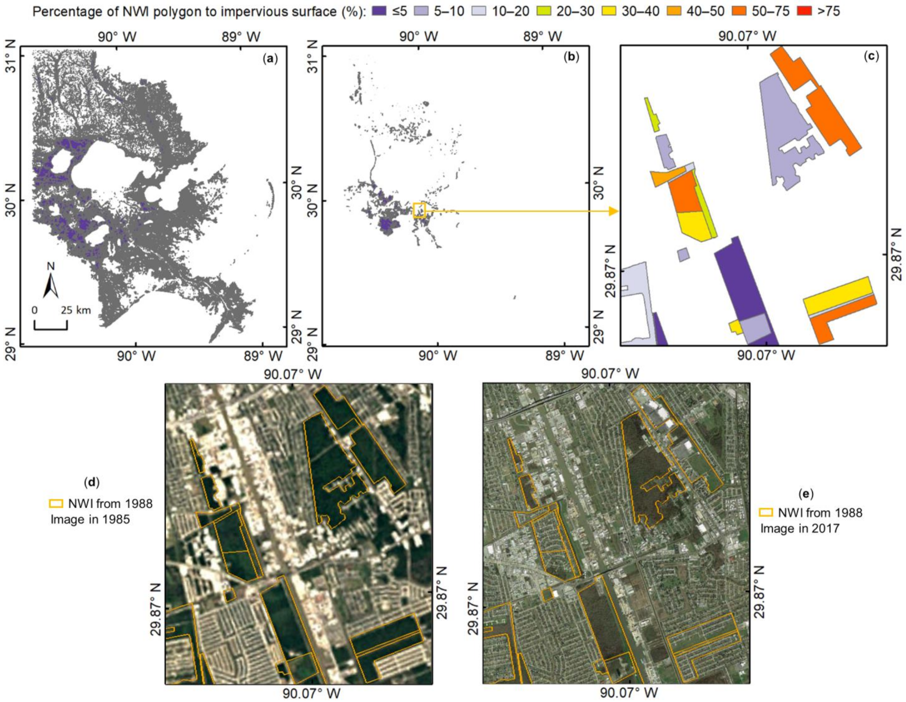
3.2. New Attributes for NWI Wetland Polygons

The two attributes of wetland loss to impervious surface for each NWI polygon are area of wetland loss (in square meters) and the percentage of this NWI polygon that experienced wetland loss. However, as most of the wetland polygons experienced no or very little wetland loss, the NWI polygons with significant wetland loss were visually overwhelmed by other NWI polygons at a small scale (Figure 5a). It is worth noting that the size of NWI polygons varies substantially, ranging from smaller than 0.01 ha to more than 10,000 ha. Selecting NWI polygons with significant wetland loss requires the use of both area and percentage of wetland loss attributes, as well as the polygon size. For the purpose of demonstration, we selected NWI polygons with significant wetland loss based on the rules that smaller wetland polygons should have a bigger percentage loss, while bigger wetland polygons can have a smaller percentage loss but require a bigger area loss. For instance, NWI polygons smaller than a half hectare should have at least 25% wetland loss, while NWI polygons larger than 500 ha should have at least 5 ha of wetland loss—in other words, at least 1% wetland loss. Based on these rules, we selected approximately 700 NWI polygons with significant wetland loss out of approximately 130,000 NWI polygons (Figure 5b). The zoomed-in view displays several NWI polygons with at least 30% wetland loss (Figure 5c). These regions were forested wetlands when the NWI polygons were created in the 1980s (Figure 5d). However, when the C-CAP dataset was created in 2017, all of these wetland polygons had undergone some degree of development, with some polygons experiencing up to 60% loss to the impervious surface (Figure 5c,e). More sophisticated rules can be defined to select polygons with significant wetland loss to meet the specific purposes of the users (for example, selecting all NWI polygons with more than 50% wetland loss).
There are three attributes used to evaluate water regime changes in drier vegetated wetlands: the area and percentage of drier vegetated wetland converted to open water, as well as the average time series DSWE inundation frequency. Since only a small percentage of these drier vegetated wetlands had significant water regime change (Figure 6a), polygons with significant water regime changes should be selected from the approximately 100,000 drier vegetated polygons. For the purpose of demonstration, a similar approach to the wetland loss polygon selection was used. For instance, a drier vegetated NWI polygon smaller than a half hectare should have at least 25% converted to open water, while a drier vegetated NWI polygon bigger than 500 ha should have at least 5 ha of open water. Based on these rules, approximately 3000 drier vegetated NWI polygons were identified with significant conversion to open surface water (Figure 6b), and around 200 of them had 100% conversion to open surface water. A zoomed-in view showed an emergent wetland with a temporarily and irregularly flooded water regime in 1988 (Figure 6d). Several decades later, it had 97.8% open water coverage according to the 2017 C-CAP dataset and an annual average DSWE inundation frequency of 98.5% from 2016 to 2018. The high-resolution image of 2016 also showed very high coverage of open water (Figure 6e).

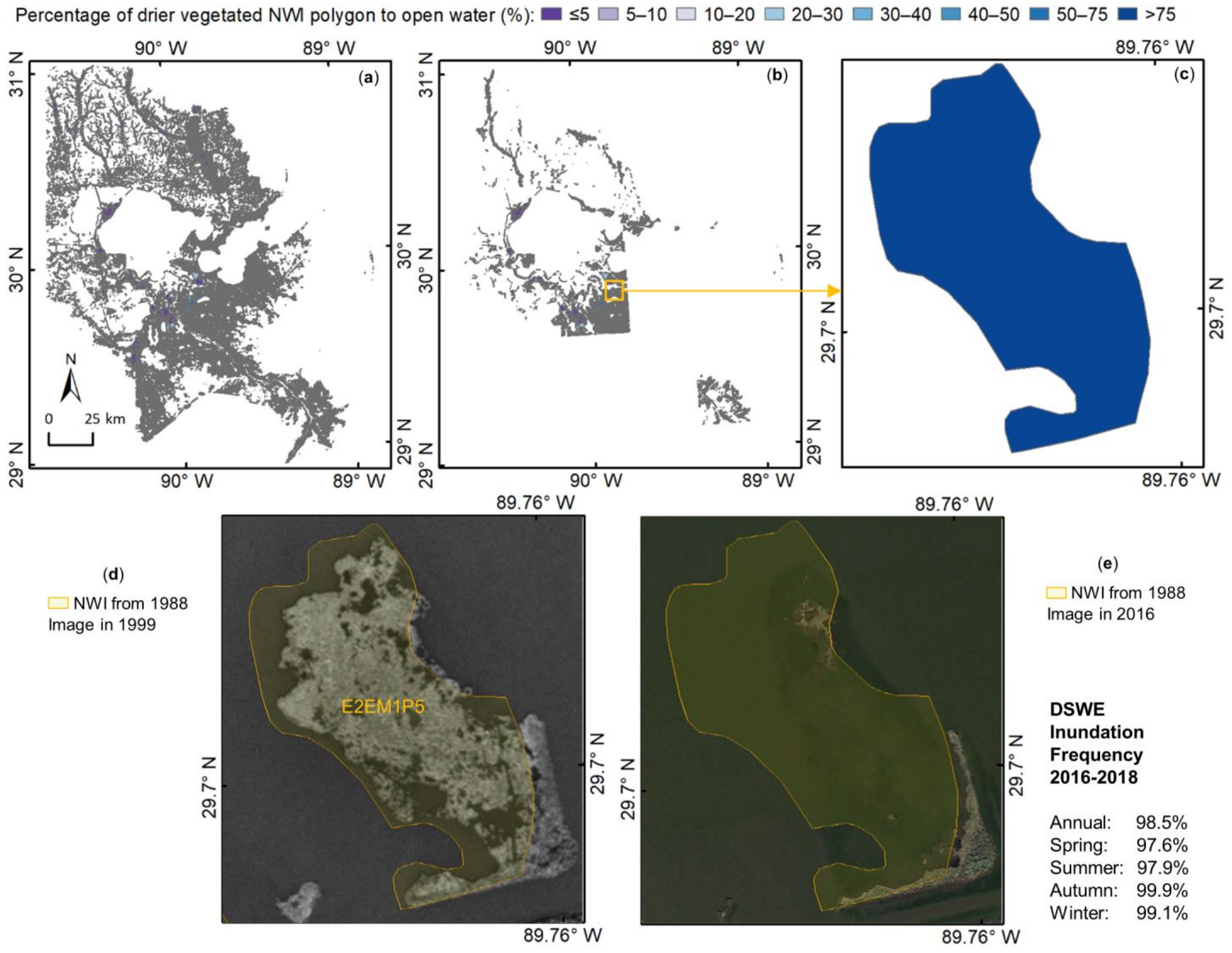
3.3. C-CAP-Based Water Body Polygons

We derived approximately 150,000 water polygons from the 1 m C-CAP dataset (Figure 7a), ranging in size from approximately 10 m2 to 70 km2. Among them, 4905 polygons were at least 30 m away from the original NWI polygons, 1634 polygons were within 30 m of the original NWI polygons, and the rest overlapped with the NWI polygons (Figure 7b). Considering that geospatial mismatch measurements for the old NWI polygons range from a few meters to 30 m (Figure 4), it is reasonable to deduce that the 4905 water polygons located at a minimum distance of 30 m from the original NWI polygons would likely experience minimal impact from potential geospatial mismatch. Consequently, these water polygons are highly likely to represent new water bodies that emerged subsequent to the creation of the old NWI. For the 1634 water polygons within a 30 m distance of the original NWI wetland polygons, they could represent new water bodies. However, they fall within the range of potential geospatial mismatches. It is possible that these water polygons have already been documented in the original NWI dataset but with a spatial shift. The water polygons overlapping with the original NWI wetland polygons are likely mapped or partly mapped in the original NWI dataset (Figure 7b). However, certain parts of these polygons could represent new water areas due to various reasons, such as the expansion of smaller NWI water bodies, the construction of reservoirs from NWI water channels, and the conversion from NWI drier vegetated wetland to open water (Figure 7b).
The attributes of time series DSWE inundation frequency were also added to these water polygons. For example, the black water polygon in Figure 7b represents a water pond with a size of 0.9 ha (Figure 7d). This water pond has an annual average DSWE inundation frequency of 89.2%, indicating that the water here is permanent.

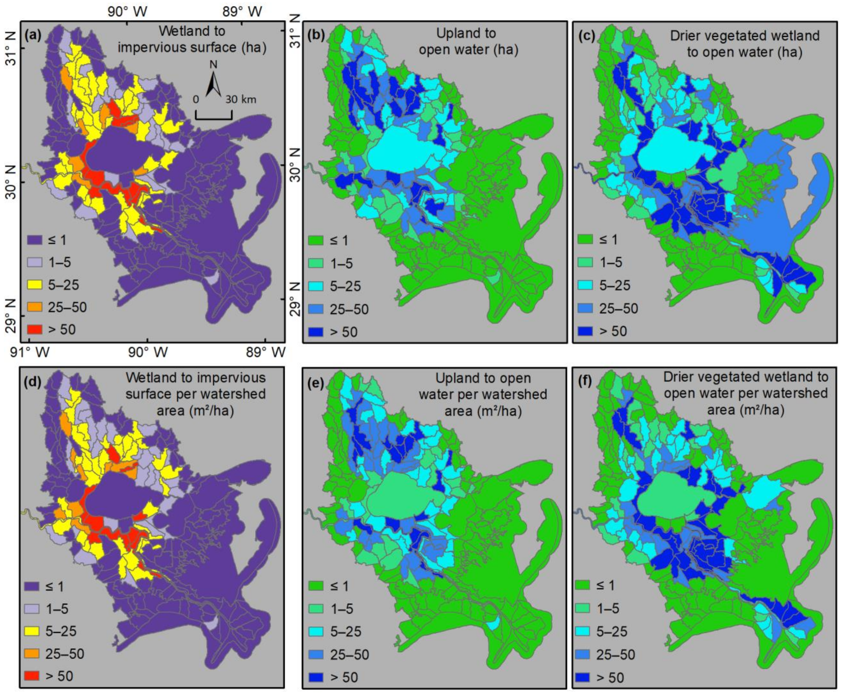
3.4. Spatially Aggregated Difference

The losses of wetlands to impervious surfaces are concentrated around the urban regions of New Orleans (Figure 8a). These watersheds have a wetland loss bigger than 50 ha (Figure 8a) or 50 square meters of wetland loss per hectare watershed area (Figure 8d). The gain of open water from upland is concentrated in the upper and middle regions of the study area. These watersheds have a new water area bigger than 50 ha (Figure 8b) or 50 square meters of new water per hectare watershed area (Figure 8e). The mining of sand and gravel may have contributed to the gain of open water in these regions [31]. The change from drier vegetated wetlands to open water is concentrated in the coastal regions. These watersheds have a water regime change bigger than 50 ha (Figure 8c) or 50 square meters of new water per hectare watershed area (Figure 8f). Sea level rise may have contributed to the permanent inundation of drier vegetated wetlands. These statistics could also be aggregated in other units such as census tracts to meet the needs of different users.

4. Discussion

Various land cover products covering portions of the U.S. and its territories are updated every few years. For example, the Multi-Resolution Land Characteristics (MRLC) Consortium of the U.S. Geological Survey (USGS) produces the National Land Cover Database (NLCD) at a 30 m resolution every 2 to 3 years [38]. The NOAA Coastal Change Analysis Program produced a land cover dataset at a 10 m resolution, covering the coastal regions of the U.S. [39]. Importantly, the NOAA Coastal Change Analysis Program will produce a 1 m resolution land cover product for coastal regions, with an update period of 4 to 6 years [26]. The information on land use and land cover change captured by these new land cover maps is useful in detecting wetland changes, which can be used to support the maintenance of the NWI geospatial dataset.
Various methods have been developed to evaluate wetland conditions and analyze wetland changes [15,17,22]. In comparison to traditional field survey methods for identifying wetland changes [15,16], our approaches are cost-efficient and can be implemented quickly. Although moderate-resolution satellite imagery and spectral analysis methods prove effective in regional-scale wetland change monitoring [17,18,19], they are unable to support NWI maintenance due to relatively low spatial resolution. In contrast, our approaches utilize 1 m C-CAP data to extract water polygons, enabling seamless support for NWI maintenance with minimal adjustments. Recent wetland studies using high-resolution data and advanced algorithms have shown great potential in their experimental study regions [20,22,23]. However, due to differing objectives, wetland classification systems, and operational procedures, the resultant wetland maps may exhibit substantial discrepancies with NWI [11], rendering them inadequate for direct NWI maintenance support. Our approaches extract information on wetland loss and open water gain from the 1 m C-CAP dataset. The results directly contribute to NWI maintenance by identifying locations with notable wetland changes across scales, spanning from 1 m pixels to NWI polygons and HUC12 watersheds.
The loss of wetland to impervious surfaces is usually considered to be permanent wetland loss, leading to huge negative impacts on local ecosystem services [40]. The area of wetland lost to impervious surfaces can be easily estimated using recent high-resolution land cover maps. However, the impacts of these wetland losses extend beyond the boundaries of impervious surfaces. Often, these wetland losses are accompanied by additional losses to non-impervious urban land, such as lawns, open spaces, parks, and golf courses. The conversion of wetlands to upland areas in these regions also has a negative impact on wetland species and wetland ecosystems, as well as the ecosystem services wetlands provide [30].
The change of upland to open water could occur in both urban and non-urban regions. In non-urban regions, new water bodies could be formed due to climate variability or the construction of reservoirs [41]. In urban regions, storm water ponds are often created to drain wetlands for development and to mitigate floods in residential regions [42]. The new water polygons extracted automatically from high-resolution land cover maps have geometric accuracy comparable to NWI polygons derived through manual delineation, meeting the NWI mapping standards. In many cases, they could be incorporated into the NWI geospatial dataset with little or no manual editing, which will greatly improve the efficiency of updating the NWI data for open water gain over upland.
High resolution land cover maps are continually being produced for more regions. For example, C-CAP 1 m data are being generated for all U.S. coastal regions [26], which will allow the derivation of difference products for those areas. Our algorithms and automated methods can be used for any regions with high-resolution land cover maps.
The changes in water regimes of NWI wetlands, such as alterations in inundation frequencies, are more subtle. As a result, it can be challenging to determine water regime changes based on images acquired at a specific date of the year due to the lack of time series inundation information. Fortunately, the availability of time series inundation information from Landsat enables a repeatable and objective approach to detect changes in water regimes, such as transitions from drier vegetated wetlands to open water. The current DSWE algorithms were developed using Landsat images [34,35]. Consequently, the resulting time series DSWE inundation data are in 30 m resolution, which can provide inundation information for medium and large NWI polygons. However, they can be too coarse for small NWI polygons, particularly those smaller than 900 m2. The U.S. Geological Survey is presently adapting the DSWE algorithms to process 10 m Sentinel-2 images. Once the algorithms have been updated, we can then generate 10 m DSWE inundation data, which will provide inundation information for smaller NWI polygons.
The new water polygons from C-CAP data, especially those with at least a 30 m distance from the original NWI polygons, could be used as initial data to produce NWI standard-compliant products. However, generating NWI products requires field sampling data and expert knowledge in wetland classification. The algorithms and products developed in this study cannot generate NWI standard products directly but can make existing workflows more efficient.

5. Conclusions

In this study, we developed algorithms and automated methods to use high-resolution C-CAP land cover mapping to support the maintenance of the NWI geospatial dataset in a rapidly evolving urban area containing New Orleans, Louisiana. Our results showed that the 1 m pixel-level difference products can pinpoint the specific locations of wetland changes, while statistics at the watershed scale can help target the regions with greatest wetland change and prioritize them for wetland maintenance. The new attributes of wetland loss and open water gain are useful in selecting wetland polygons with the most significant changes from thousands of wetland polygons. The new water polygons derived from the C-CAP dataset have good quality geometry and can serve as initial inputs for producing standard-compliant NWI products. The methods, algorithms, and products developed in this study demonstrate the feasibility of using high-resolution land cover maps to support the maintenance of the NWI geospatial dataset, speeding up the updating processes while reducing costs. The findings can benefit researchers, policymakers, and conservationists who rely on NWI data for wetland research, conservation, and management. Future directions include testing the proposed approaches in other regions and developing high-resolution time series inundation frequency products.

Author Contributions

Z.Z., C.H. and M.W.L. designed the study. Z.Z. carried out algorithm writing, data processing, product generation and validation in close discussion with C.H. and M.W.L., Z.Z., C.H., M.W.L., L.D. and G.M. led the interpretation of the results and the writing of the manuscript. J.C.I. and R.G. provided the National Wetlands Inventory dataset and attribute list of drier vegetated wetland. N.H. provided the Coastal Change Analysis Program dataset. L.D., G.M., J.C.I., R.G. and N.H. contributed to the analysis of the dataset. W.G. and J.L. contributed to data processing and result interpretation. All listed authors contributed to the writing and editing of the manuscript. All authors have read and agreed to the published version of the manuscript.

Funding

This study was funded by the U.S. Fish and Wildlife Service (USFWS) under contract F20AC11249 and supported in part by the U.S. Department of Agriculture (USDA) Natural Resources Conservation Service under their Conservation Effects Assessment Project (CEAP).

Data Availability Statement

The code to generate the difference products can be found on GitHub at the following link: https://github.com/ZhenhuaZou/new_orleans (accessed on 1 June 2023).

Acknowledgments

The authors would like to acknowledge the Google Earth Engine (GEE) cloud computing platform and Alphabet Inc. for the free computation power and huge data storage, making it possible to analyze a large volume of remote sensing data in a short time. The findings and conclusions in this article are those of the authors and do not necessarily represent the views of the U.S. Fish and Wildlife Service. The use of trade, firm, or product names is for descriptive purposes only and does not imply endorsement by the U.S. Government.

Conflicts of Interest

The authors declare no conflict of interest.

References

  1. Mitsch, W.J.; Bernal, B.; Hernandez, M.E. Ecosystem Services of Wetlands. Int. J. Biodivers. Sci. Ecosyst. Serv. Manag. 2015, 11, 1–4. [Google Scholar] [CrossRef]
  2. Murray, N.J. The Extent and Drivers of Global Wetland Loss. Nature 2023, 614, 234–235. [Google Scholar] [CrossRef] [PubMed]
  3. Galatowitsch, S.M. Natural and Anthropogenic Drivers of Wetland Change. In The Wetland Book Ii: Distribution, Description, and Conservation; Springer Nature: London, UK, 2018; pp. 359–367. [Google Scholar]
  4. Senanayake, I.P.; Yeo, I.Y.; Kuczera, G.A. A Random Forest-Based Multi-Index Classification (Rafmic) Approach to Mapping Three-Decadal Inundation Dynamics in Dryland Wetlands Using Google Earth Engine. Remote Sens. 2023, 15, 1263. [Google Scholar] [CrossRef]
  5. Sudol, T.A.; Noe, G.B.; Reed, D.J. Tidal Wetland Resilience to Increased Rates of Sea Level Rise in the Chesapeake Bay: Introduction to the Special Feature. Wetlands 2020, 40, 1667–1671. [Google Scholar] [CrossRef]
  6. Russell, M.T.; Cartwright, J.M.; Collins, G.H.; Long, R.A.; Eitel, J.H. Legacy Effects of Hydrologic Alteration in Playa Wetland Responses to Droughts. Wetlands 2020, 40, 2011–2024. [Google Scholar] [CrossRef]
  7. Johnson, W.C.; Poiani, K.A. Climate Change Effects on Prairie Pothole Wetlands: Findings from a Twenty-Five Year Numerical Modeling Project. Wetlands 2016, 36, 273–285. [Google Scholar] [CrossRef]
  8. Jamal, S.; Ahmad, W.S. Assessing Land Use Land Cover Dynamics of Wetland Ecosystems Using Landsat Satellite Data. SN Appl. Sci. 2020, 2, 1891. [Google Scholar] [CrossRef]
  9. Wang, Y.; Molinos, J.G.; Shi, L.; Zhang, M.; Wu, Z.; Zhang, H.; Xu, J. Drivers and Changes of the Poyang Lake Wetland Ecosystem. Wetlands 2019, 39, 35–44. [Google Scholar] [CrossRef]
  10. Gibbs, J.P. Wetland Loss and Biodiversity Conservation. Conserv. Biol. 2000, 14, 314–317. [Google Scholar] [CrossRef]
  11. Matthews, J.W.; Skultety, D.; Zercher, B.; Ward, M.P.; Benson, T.J. Field Verification of Original and Updated National Wetlands Inventory Maps in Three Metropolitan Areas in Illinois, USA. Wetlands 2016, 36, 1155–1165. [Google Scholar] [CrossRef]
  12. Dahl, T.; Bergeson, M. Technical Procedures for Conducting Status and Trends of the Nation’s Wetlands; U.S. Department of the Interior, U.S. Fish and Wildlife Service: Washington, DC, USA, 2017. Available online: https://www.fws.gov/wetlands/documents/Technical-Procedures-for-Conducting-Status-and-Trends-of-the-Nations-Wetlands.pdf (accessed on 10 December 2022).
  13. Hu, S.; Niu, Z.; Chen, Y. Global Wetland Datasets: A Review. Wetlands 2017, 37, 807–817. [Google Scholar] [CrossRef]
  14. Federal Geographic Data Committee. Classification of Wetlands and Deepwater Habitats of the United States; Federal Geographic Data Committee and U.S. Fish and Wildlife Service: Washington, DC, USA, 2013. Available online: https://www.fws.gov/sites/default/files/documents/Classification-of-Wetlands-and-Deepwater-Habitats-of-the-United-States-2013.pdf (accessed on 20 September 2020).
  15. Holland, C.C.; Honea, J.E.; Gwin, S.E.; Kentula, M.E. Wetland Degradation and Loss in the Rapidly Urbanizing Area of Portland, Oregon. Wetlands 1995, 15, 336–345. [Google Scholar] [CrossRef]
  16. Kentula, M.E.; Gwin, S.E.; Pierson, S.M. Tracking Changes in Wetlands with Urbanization: Sixteen Years of Experience in Portland, Oregon, USA. Wetlands 2004, 24, 734–743. [Google Scholar] [CrossRef]
  17. Houhoulis, P.F.; Michener, W.K. Detecting Wetland Change: A Rule-Based Approach Using Nwi and Spot-Xs Data. Photogramm. Eng. Remote Sens. 2000, 66, 205–211. [Google Scholar]
  18. Dobson, J.E. Noaa Coastal Change Analysis Program (C-Cap): Guidance for Regional Implementation. 1995. Available online: https://spo.nmfs.noaa.gov/Technical%20Report/tr123.pdf (accessed on 10 August 2023).
  19. Nielsen, E.M.; Prince, S.D.; Koeln, G.T. Wetland Change Mapping for the Us Mid-Atlantic Region Using an Outlier Detection Technique. Remote Sens. Environ. 2008, 112, 4061–4074. [Google Scholar] [CrossRef]
  20. Xu, H.Q.; Toman, E.M.; Zhao, K.G.; Baird, J. Fusion of Lidar and Aerial Imagery to Map Wetlands and Channels Via Deep Convolutional Neural Network. Transp. Res. Rec. 2022, 2676, 374–381. [Google Scholar] [CrossRef]
  21. Stein, B.R.; Zheng, B.J.J.; Kikkinidis, I.; Kayastha, N.; Seigler, T.; Gokkaya, K.; Gopalakrishnan, R.; Hwang, W.H. An Efficient Remote Sensing Solution to Update the Ncwi. Photogramm. Eng. Remote Sens. 2012, 78, 537–547. [Google Scholar]
  22. Wu, Q.S.; Lane, C.R.; Li, X.C.; Zhao, K.G.; Zhou, Y.Y.; Clinton, N.; DeVries, B.; Golden, H.E.; Lang, M.W. Integrating Lidar Data and Multi-Temporal Aerial Imagery to Map Wetland Inundation Dynamics Using Google Earth Engine. Remote Sens. Environ. 2019, 228, 1–13. [Google Scholar] [CrossRef]
  23. Du, L.; McCarty, G.W.; Zhang, X.; Lang, M.W.; Vanderhoof, M.K.; Li, X.; Huang, C.; Lee, S.; Zou, Z. Mapping Forested Wetland Inundation in the Delmarva Peninsula, USA Using Deep Convolutional Neural Networks. Remote Sens. 2020, 12, 644. [Google Scholar] [CrossRef]
  24. Whitcomb, J.; Moghaddam, M.; McDonald, K.; Kellndorfer, J.; Podest, E. Mapping Vegetated Wetlands of Alaska Using L-Band Radar Satellite Imagery. Can. J. Remote Sens. 2009, 35, 54–72. [Google Scholar] [CrossRef]
  25. Stubbs, Q.; Yeo, I.Y.; Lang, M.G.; Townshend, J.; Sun, L.X.; Prestegaard, K.; Jantz, C. Assessment of Wetland Change on the Delmarva Peninsula from 1984 to 2010. J. Coastal. Res. 2020, 36, 575–589. [Google Scholar] [CrossRef]
  26. NOAA. High Resolution Land Cover Data. Coastal Change Analysis Program (C-Cap) High-Resolution Land Cover; Noaa Office for Coastal Management: Charleston, SC, USA, 2022. Available online: https://chs.coast.noaa.gov/htdata/raster1/landcover/bulkdownload/hires/la/ (accessed on 5 January 2022).
  27. Barbier, E.B.; Georgiou, I.Y.; Enchelmeyer, B.; Reed, D.J. The Value of Wetlands in Protecting Southeast Louisiana from Hurricane Storm Surges. PLoS ONE 2013, 8, e58715. [Google Scholar] [CrossRef] [PubMed]
  28. Jankowski, K.L.; Tornqvist, T.E.; Fernandes, A.M. Vulnerability of Louisiana’s Coastal Wetlands to Present-Day Rates of Relative Sea-Level Rise. Nat. Commun. 2017, 8, 14792. [Google Scholar] [CrossRef] [PubMed]
  29. Lane, R.R.; Day, J.W.; Day, J.N. Wetland Surface Elevation, Vertical Accretion, and Subsidence at Three Louisiana Estuaries Receiving Diverted Mississippi River Water. Wetlands 2006, 26, 1130–1142. [Google Scholar] [CrossRef]
  30. Ehrenfeld, J.G. Evaluating Wetlands within an Urban Context. Ecol. Eng. 2000, 15, 253–265. [Google Scholar] [CrossRef]
  31. Mossa, J.; Marks, S.R. Pit Avulsions and Planform Change on a Mined River Floodplain: Tangipahoa River, Louisiana. Phys. Geogr. 2011, 32, 512–532. [Google Scholar] [CrossRef]
  32. Cowardin, L.M.; Carter, V.; Golet, F.C.; LaRoe, E.T. Classification of Wetlands and Deepwater Habitats of the United States, 1st ed.; US Department of the Interior, US Fish and Wildlife Service: Washington, DC, USA, 1979; pp. 21–24.
  33. U.S. Fish and Wildlife Service. National Wetland Inventory. 2021. Available online: https://fwsprimary.wim.usgs.gov/wetlands/apps/wetlands-mapper/ (accessed on 20 July 2021).
  34. Jones, J.W. Efficient Wetland Surface Water Detection and Monitoring Via Landsat: Comparison with in Situ Data from the Everglades Depth Estimation Network. Remote Sens. 2015, 7, 12503–12538. [Google Scholar] [CrossRef]
  35. Jones, J.W. Improved Automated Detection of Subpixel-Scale Inundationrevised Dynamic Surface Water Extent (Dswe) Partial Surface Water Tests. Remote Sens. 2019, 11, 374. [Google Scholar] [CrossRef]
  36. Gorelick, N.; Hancher, M.; Dixon, M.; Ilyushchenko, S.; Thau, D.; Moore, R. Google Earth Engine: Planetary-Scale Geospatial Analysis for Everyone. Remote Sens. Environ. 2017, 202, 18–27. [Google Scholar] [CrossRef]
  37. McKinney, M.L. Urbanization, Biodiversity, and Conservation. Bioscience 2002, 52, 883–890. [Google Scholar] [CrossRef]
  38. Wickham, J.; Stehman, S.V.; Sorenson, D.G.; Gass, L.; Dewitz, J.A. Thematic Accuracy Assessment of the Nlcd 2016 Land Cover for the Conterminous United States. Remote Sens. Environ. 2021, 257, 112357. [Google Scholar] [CrossRef]
  39. NOAA. C-Cap Land Cover Files for 10 m Land Cover. 2017. Available online: https://coast.noaa.gov/htdata/raster1/landcover/bulkdownload/Beta/10m_LC/ (accessed on 3 November 2022).
  40. Wang, X.G.; Yan, F.Q.; Su, F.Z. Impacts of Urbanization on the Ecosystem Services in the Guangdong-Hong Kong-Macao Greater Bay Area, China. Remote Sens. 2020, 12, 3269. [Google Scholar] [CrossRef]
  41. Zou, Z.; Xiao, X.; Dong, J.; Qin, Y.; Doughty, R.B.; Menarguez, M.A.; Zhang, G.; Wang, J. Divergent Trends of Open-Surface Water Body Area in the Contiguous United States from 1984 to 2016. Proc. Natl. Acad. Sci. USA 2018, 115, 3810–3815. [Google Scholar] [CrossRef] [PubMed]
  42. Skovira, L.M.; Bohlen, P.J. Water Quality, Vegetation, and Management of Stormwater Ponds Draining Three Distinct Urban Land Uses in Central Florida. Urban Ecosyst. 2023, 26, 867–879. [Google Scholar] [CrossRef]
Figure 1. Study area. (a) Study area boundary overlaid on U.S. state boundary. (b) NWI project years of the study area. (c) C-CAP land cover map of the study area.
Remotesensing 15 04075 g001
Figure 2. Flow chart of this study.
Remotesensing 15 04075 g002
Figure 3. Pixel level difference product: (a) difference product of the entire study area, (b) zoomed-in area, (c) NWI (created in 1988 with an attribute of PFO1/4A) overlaid on image from 1998 of the zoomed-in area, and (d) NWI overlaid on image from 2017 of the zoomed-in area.
Remotesensing 15 04075 g003
Figure 4. Geospatial mismatches: (a) the geospatial mismatch distance of several random locations, (b) a zoomed-in view of an NWI polygon overlaid on a 2019 high-resolution image (there is a geospatial mismatch distance of 18 m), and (c) a zoomed-in view of the same NWI polygon overlaid on a 1977 high-resolution image.
Remotesensing 15 04075 g004
Figure 5. Statistics of wetland loss at NWI feature scale: (a) percentage of NWI polygon to impervious surface, (b) selected NWI polygons with significant wetland loss, (c) zoom-in of the selected NWI polygons (created in 1988), (d) selected NWI polygons overlaid on image from 1985 of the zoom-in, and (e) selected NWI polygons overlaid on image from 2017 of the zoom-in.
Remotesensing 15 04075 g005
Figure 6. Statistics of open water gain in drier vegetated NWI polygons: (a) percentage of drier vegetated NWI polygon (created in 1988) to open water, (b) selected NWI polygons with significant open water gain, (c) zoomed-in view of the selected NWI polygon, (d) the selected NWI polygon overlaid on image from 1999, and (e) the selected NWI polygon overlaid on image from 2016. The annual and seasonal DSWE inundation frequencies of the selected NWI polygon were also shown.
Remotesensing 15 04075 g006
Figure 7. Water polygons from C-CAP dataset: (a) water polygons from C-CAP dataset and their distances from original NWI polygons, (b) zoomed-in (DSWE information is shown for the black polygon in upper right), (c) original NWI polygon (created in 1976) overlaid on image from 1999 of the zoomed-in view, and (d) original NWI polygon overlaid on image in 2017 of the zoomed-in view.
Remotesensing 15 04075 g007
Figure 8. Statistics of wetland change at HUC12 watershed scale: (a) Wetland to impervious surface (ha), (b) upland to open water (ha), (c) drier vegetated wetland to open water (ha), (d) wetland to impervious surface per watershed area (m2/ha), (e) upland to open water per watershed area (m2/ha), and (f) drier vegetated wetland to open water per watershed area (m2/ha).
Remotesensing 15 04075 g008
Table 1. Water regime codes and their full names [32].
NontidalSaltwater TidalFreshwater Tidal
CodeNameCodeNameCodeName
ATemporarily FloodedLSubtidalQRegularly Flooded–Fresh Tidal
BSeasonally SaturatedMIrregularly ExposedRSeasonally Flooded–Fresh Tidal
CSeasonally FloodedNRegularly FloodedSTemporarily Flooded–Fresh Tidal
DContinuously SaturatedPIrregularly FloodedTSemi-Permanently Flooded–Fresh Tidal
ESeasonally Flooded/Saturated VPermanently Flooded–Fresh Tidal
FSemi-Permanently Flooded
GIntermittently Exposed
HPermanently Flooded
JIntermittently Flooded
KArtificially Flooded
Table 2. Confusion matrix of wetland to impervious surface.
Reference Data
Wetland to Impervious (Reference)Wetland Not Changed to Impervious (Reference)TotalUser Accuracy
Wetland to impervious (map)185152000.925
Wetland not changed to impervious (map)02002001.000
Total185215400Overall Accuracy
Producer accuracy1.0000.930 0.963
Table 3. Confusion matrix of upland to open water.
Upland to Open Water (Reference)Upland Not Changed to Water (Reference)TotalUser Accuracy
Upland to Open water (map)19732000.985
Upland not changed to water (map)11992000.995
Total198202400Overall Accuracy
Producer accuracy0.9950.985 0.990
Table 4. Confusion matrix of drier vegetated wetland to open water.
Drier Vegetated Wetland to Open Water (Reference)Drier Vegetated Wetland Not Changed to Open Water (Reference)TotalUser Accuracy
Driver vegetated wetland to open water (map)189112000.945
Driver vegetated wetland not changed to open water (map)151852000.925
Total204196400Overall Accuracy
Producer accuracy0.9260.944 0.935
Disclaimer/Publisher’s Note: The statements, opinions and data contained in all publications are solely those of the individual author(s) and contributor(s) and not of MDPI and/or the editor(s). MDPI and/or the editor(s) disclaim responsibility for any injury to people or property resulting from any ideas, methods, instructions or products referred to in the content.

