


A Spatial Data-Driven Approach for Mineral Prospectivity Mapping

 ,
,  , and
, and
Abstract
:
1. Introduction
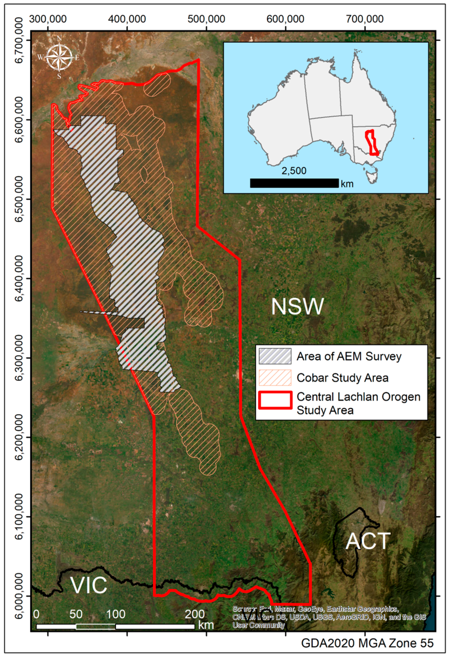
2. Study Area
- Rift phase deposition and widespread volcanism in discrete volcanic troughs/belts ca. 420 Ma;
- Transition to sag phase deposition at ca. 410 Ma, with stable sag phase deposition continuing until ca. 400 Ma. Bindian extension/contraction at ca. 410 Ma; and
- Inversion phase during the Tabberabberan Orogeny ca. 390–380 Ma.
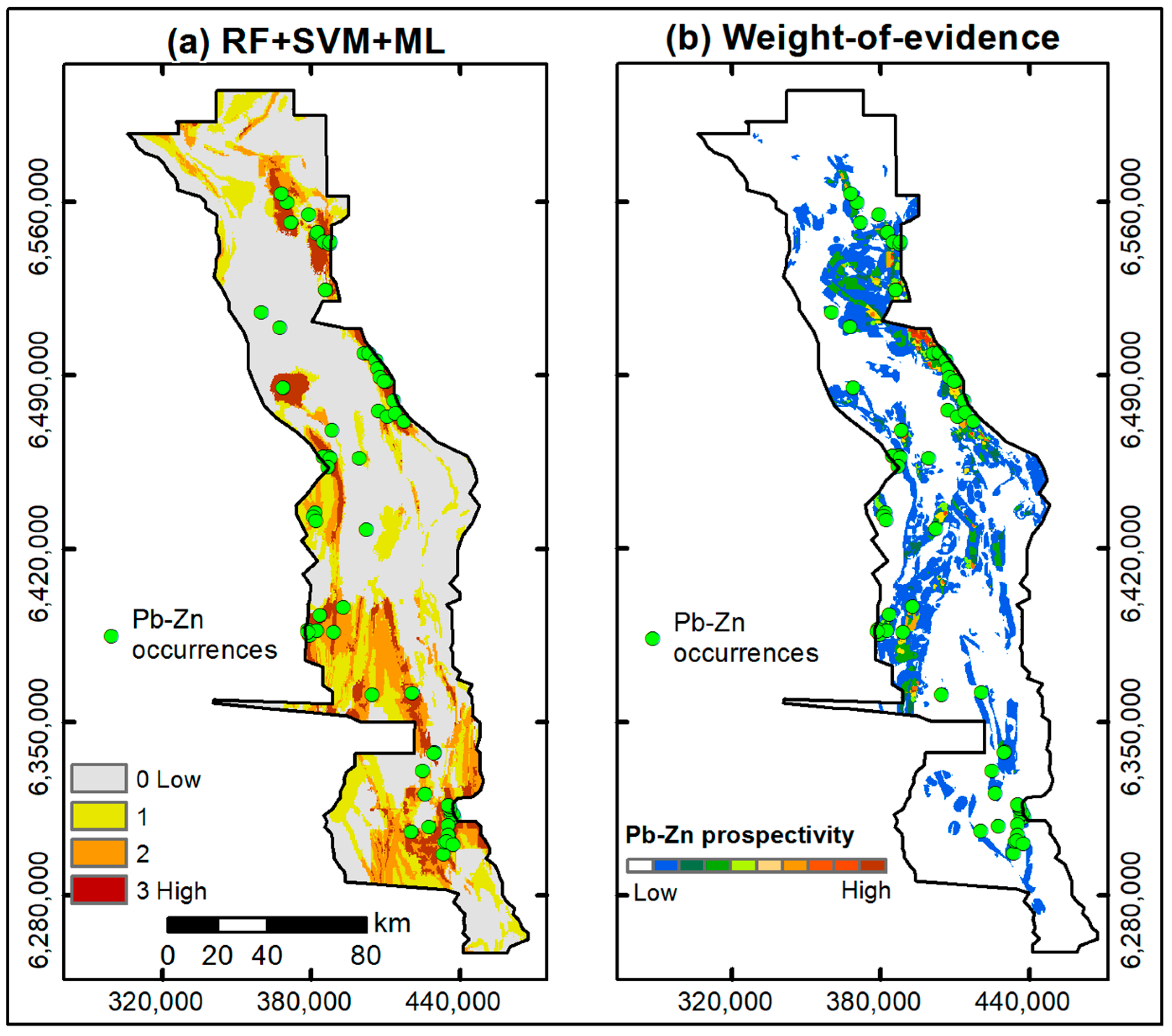
2.1. Mineral Prospectivity Mapping in Central Lachlan Orogen Using WofE Method
3. Methodology
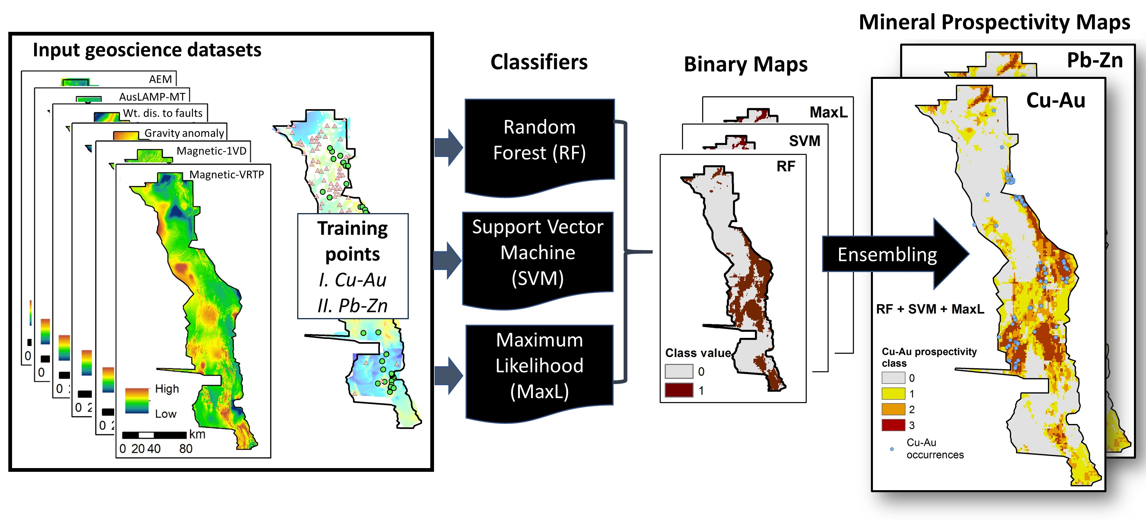
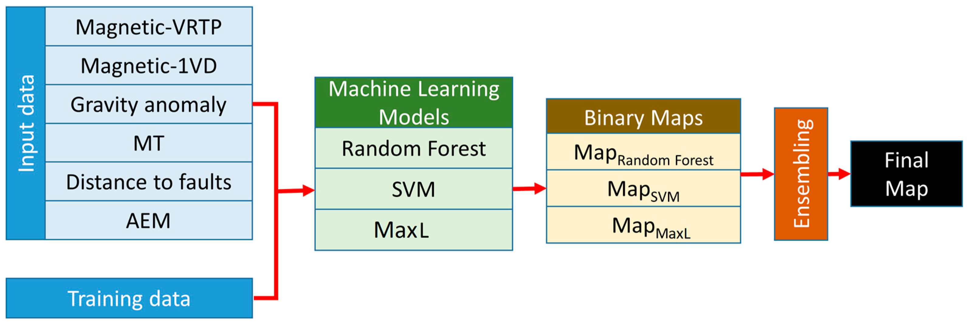
3.1. Overview of the Methodology
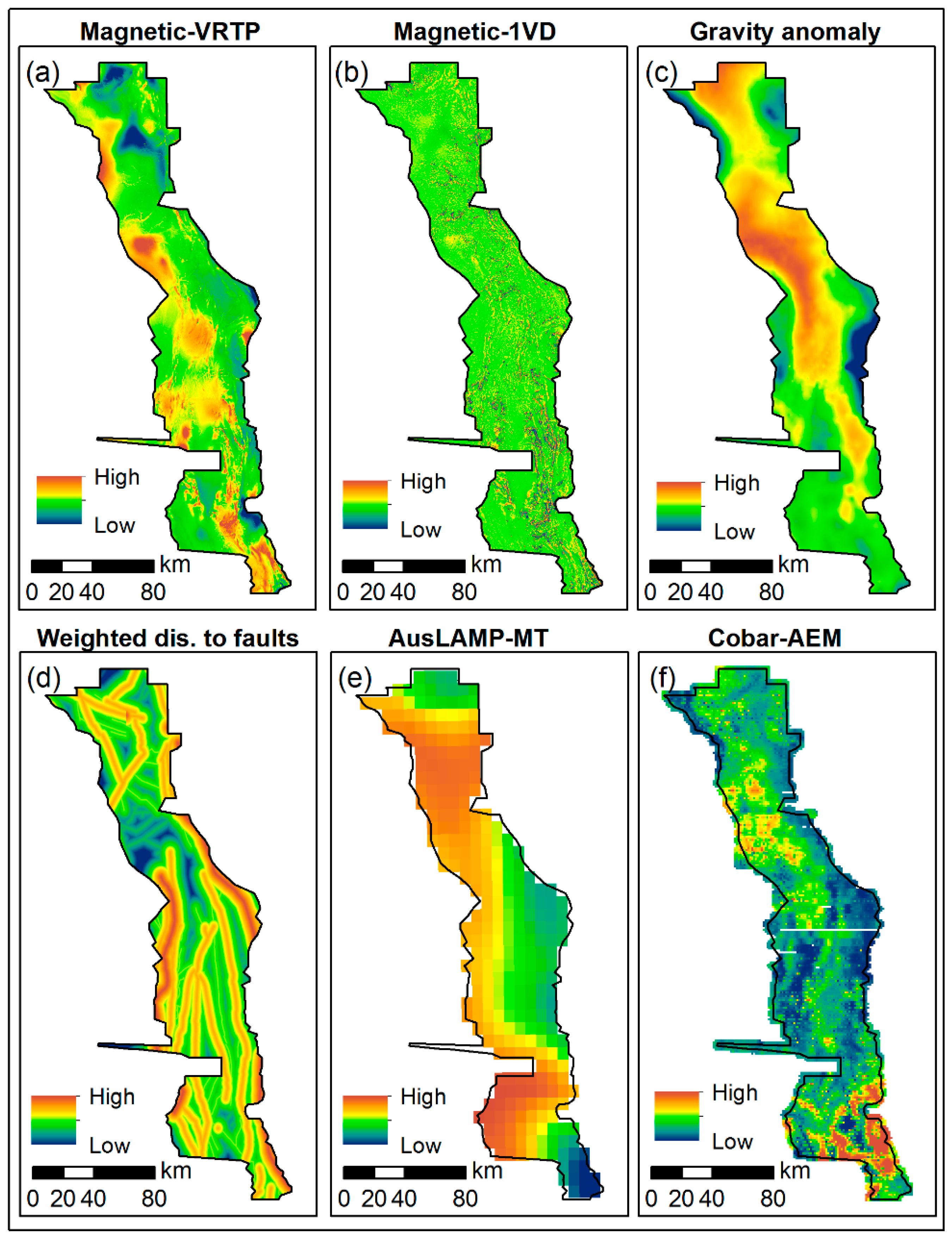
3.2. Datasets
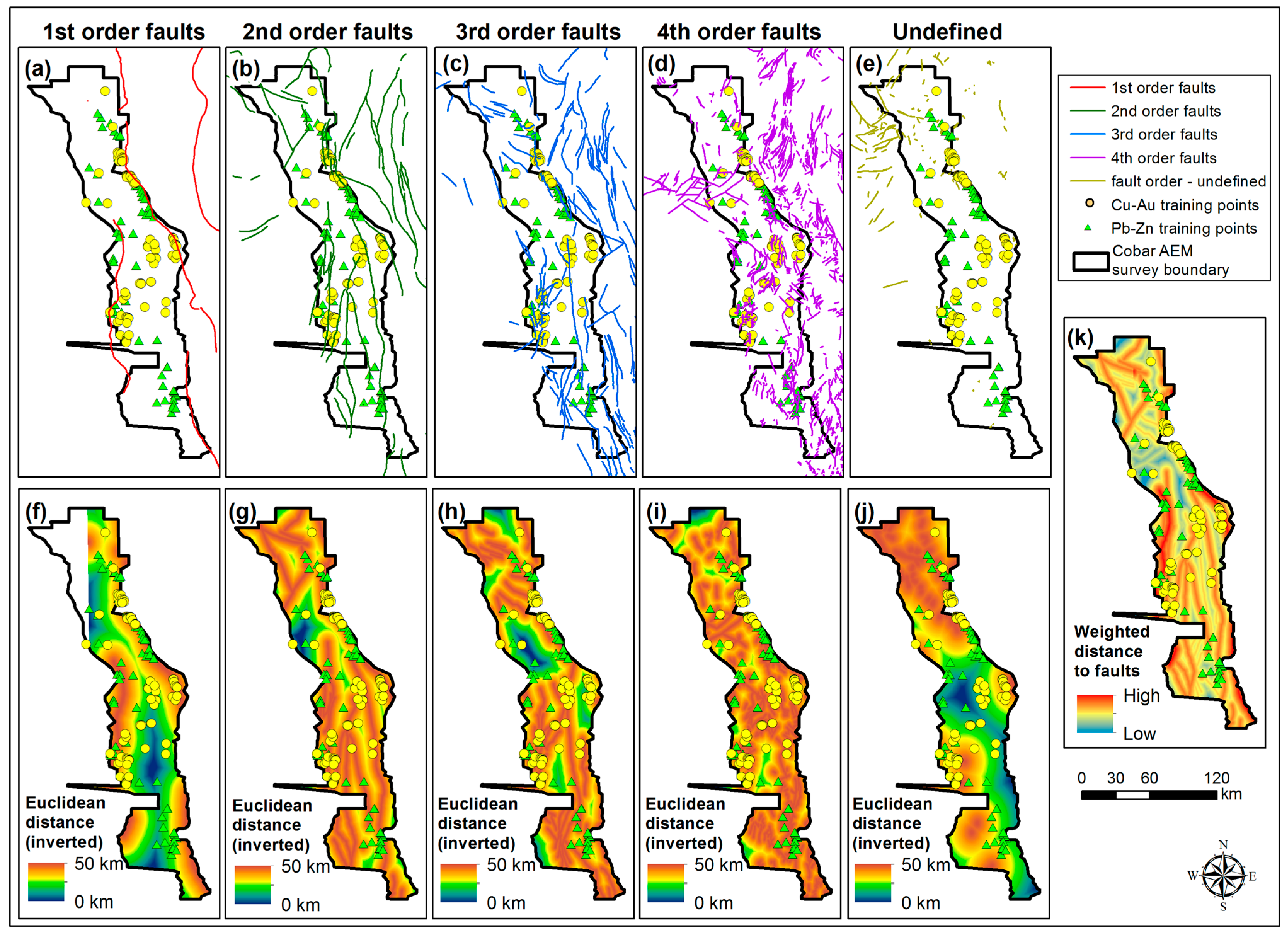
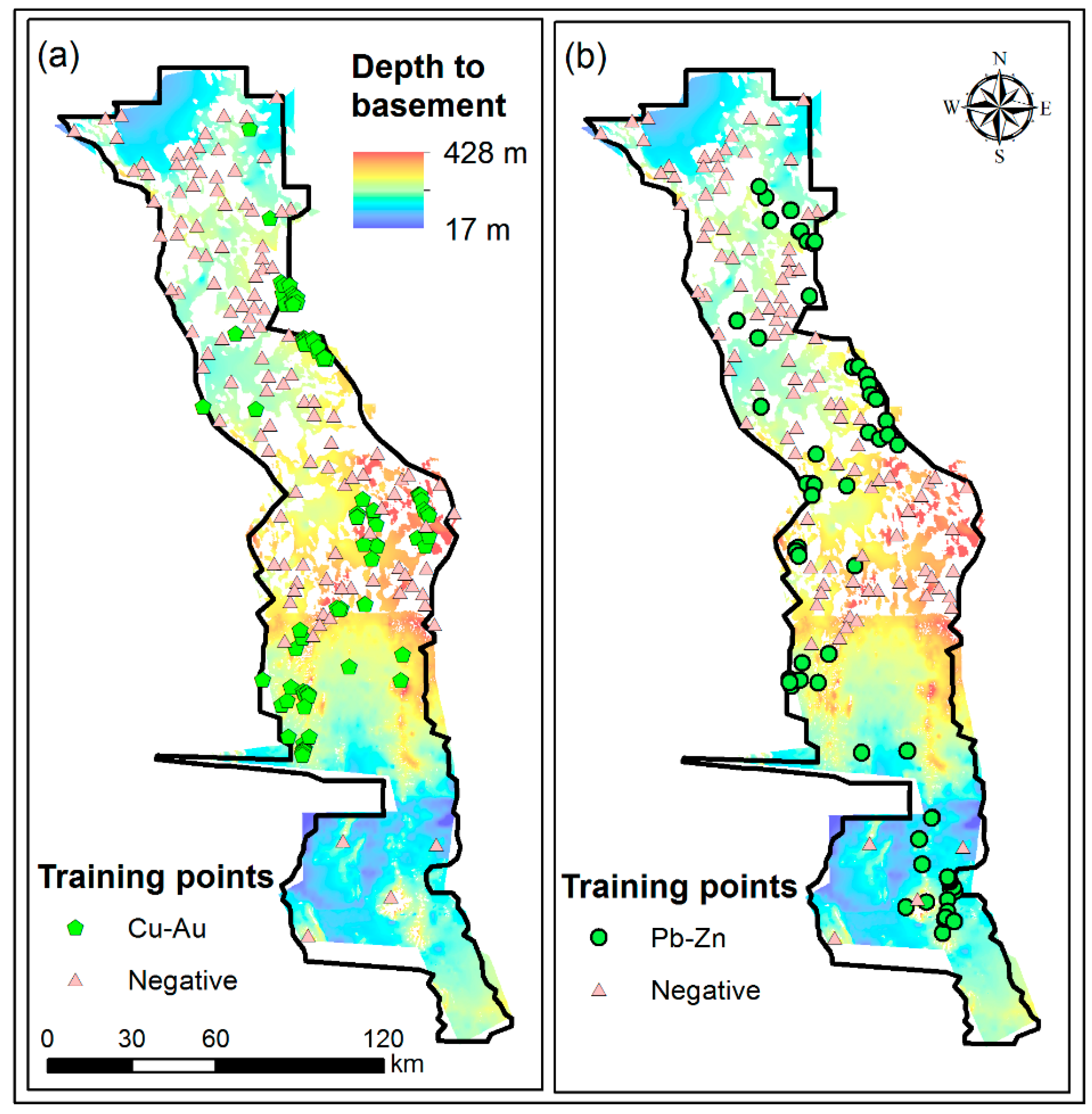
3.3. Data Pre-Processing
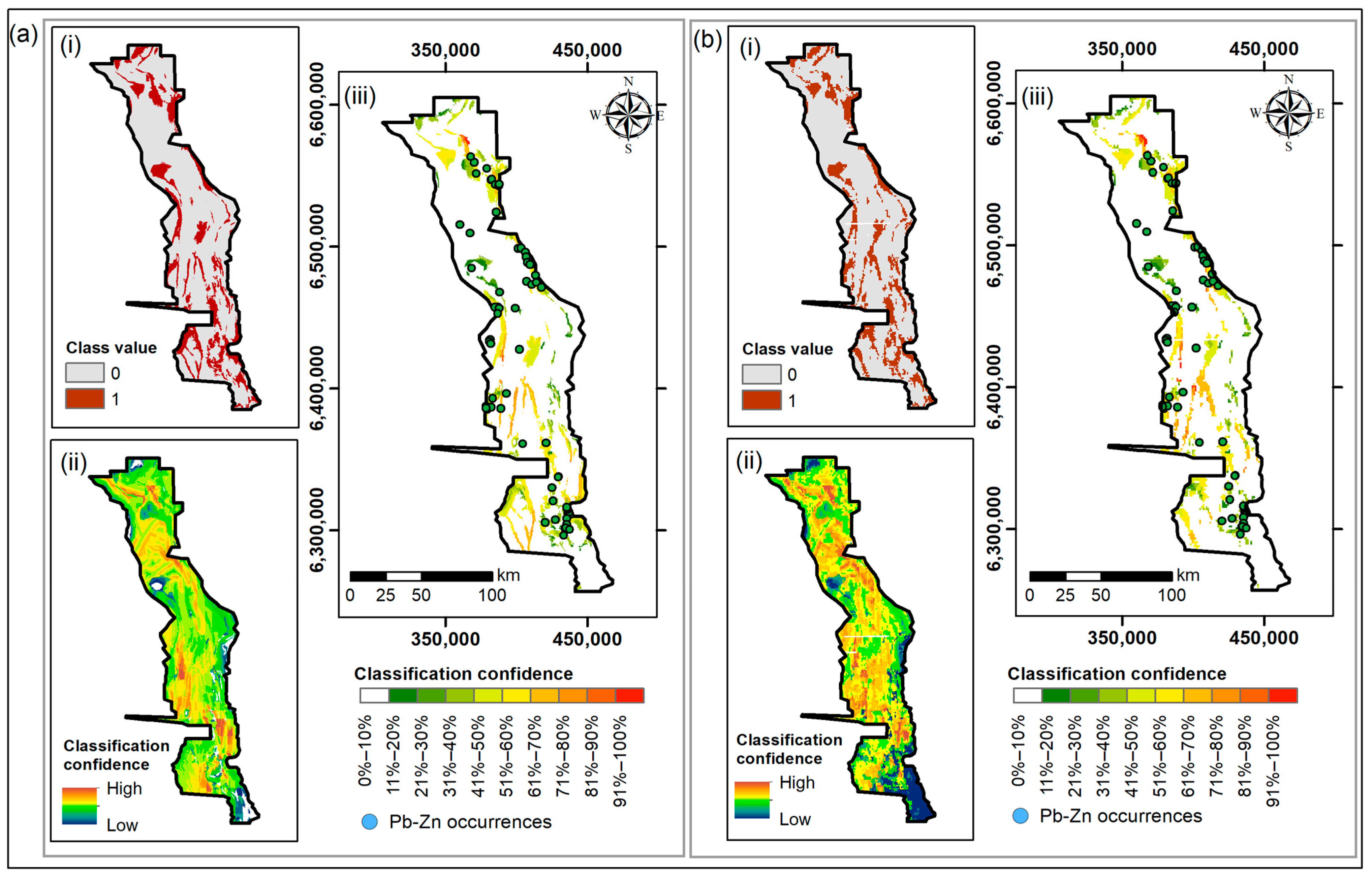
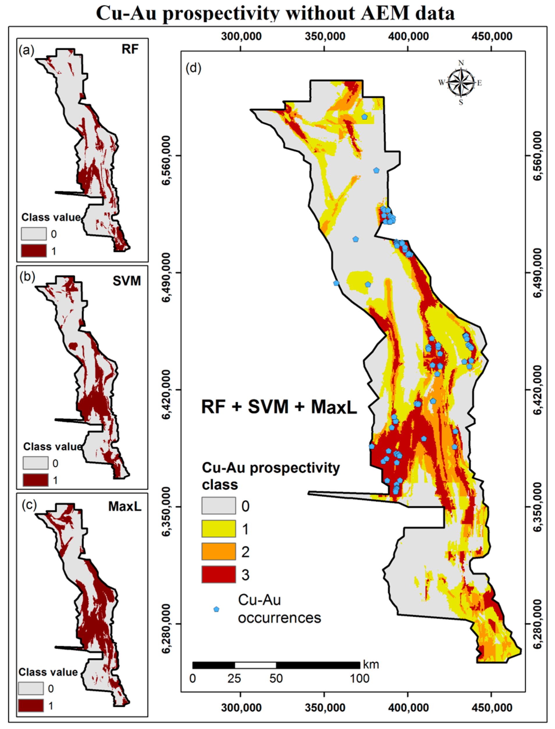
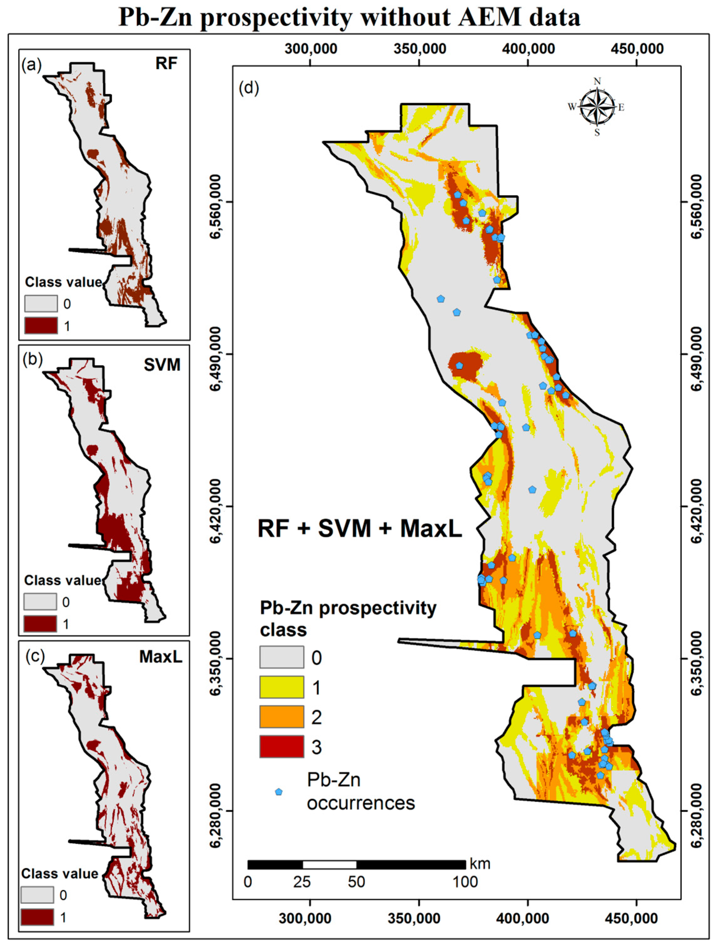
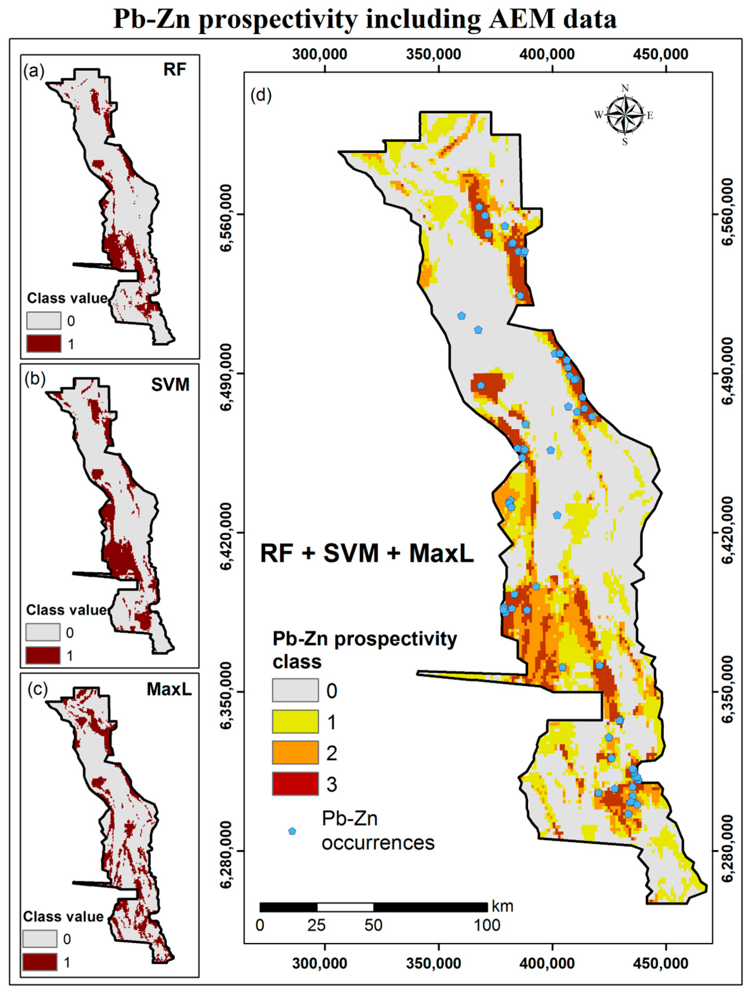
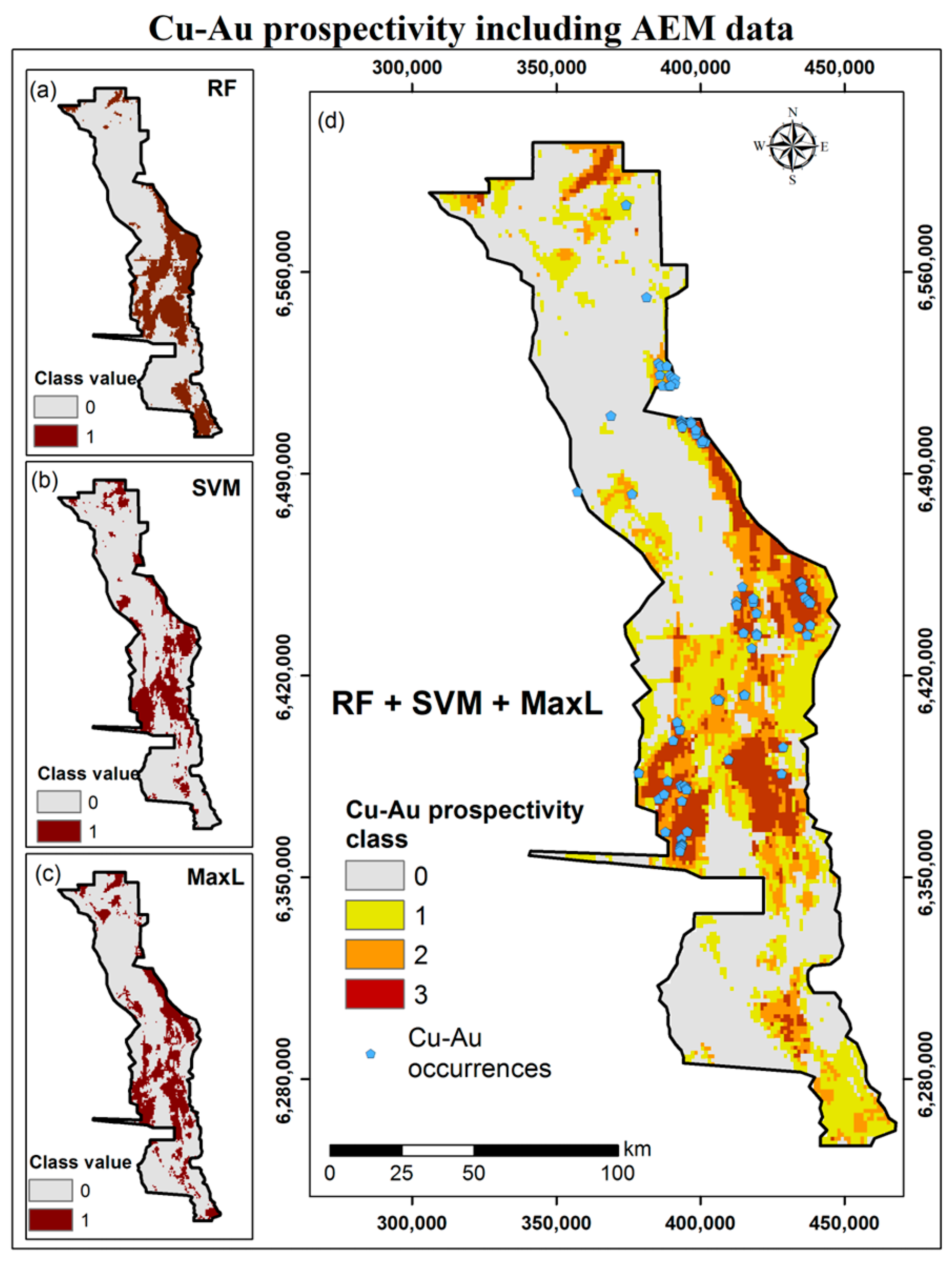
3.4. Classification
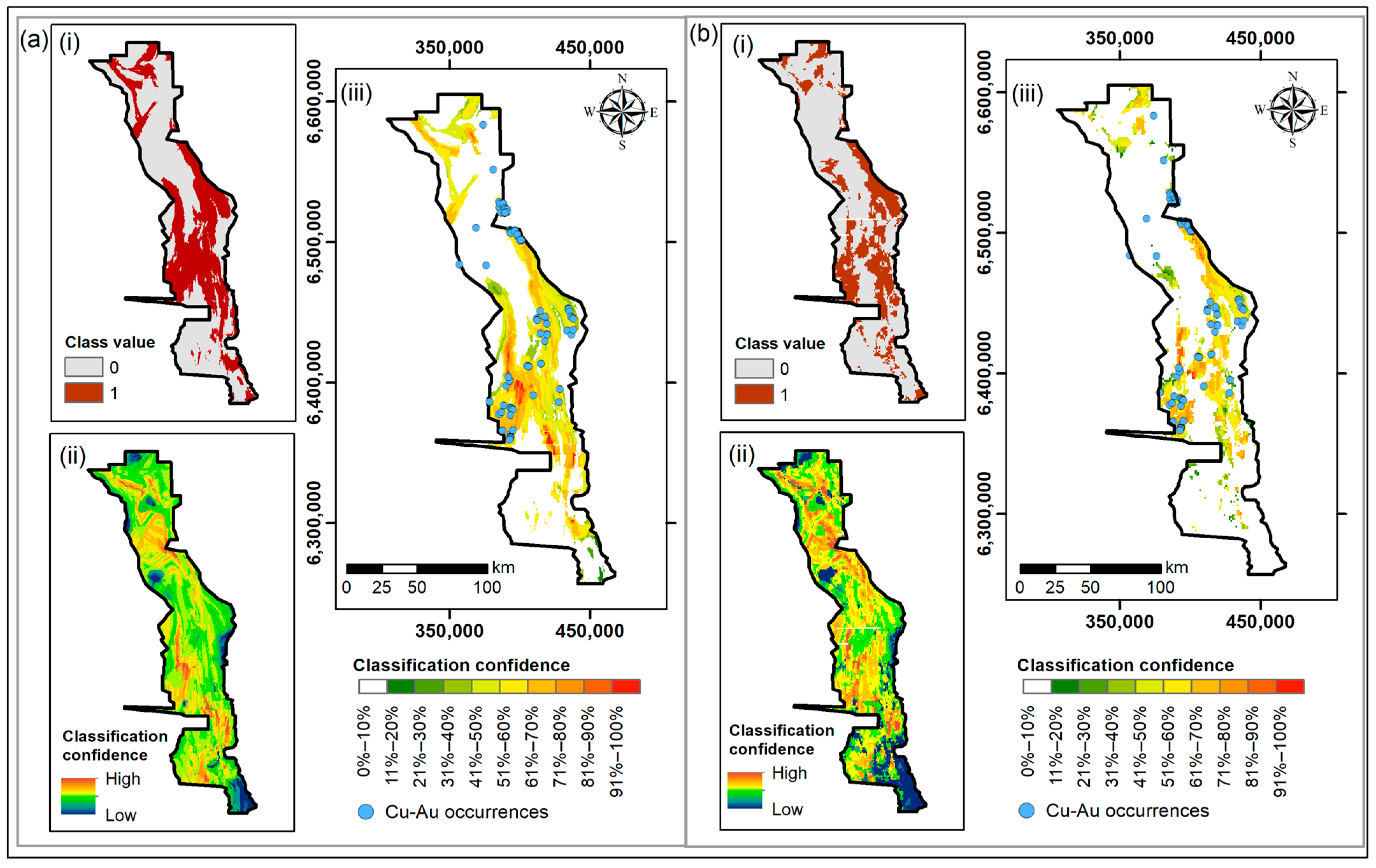
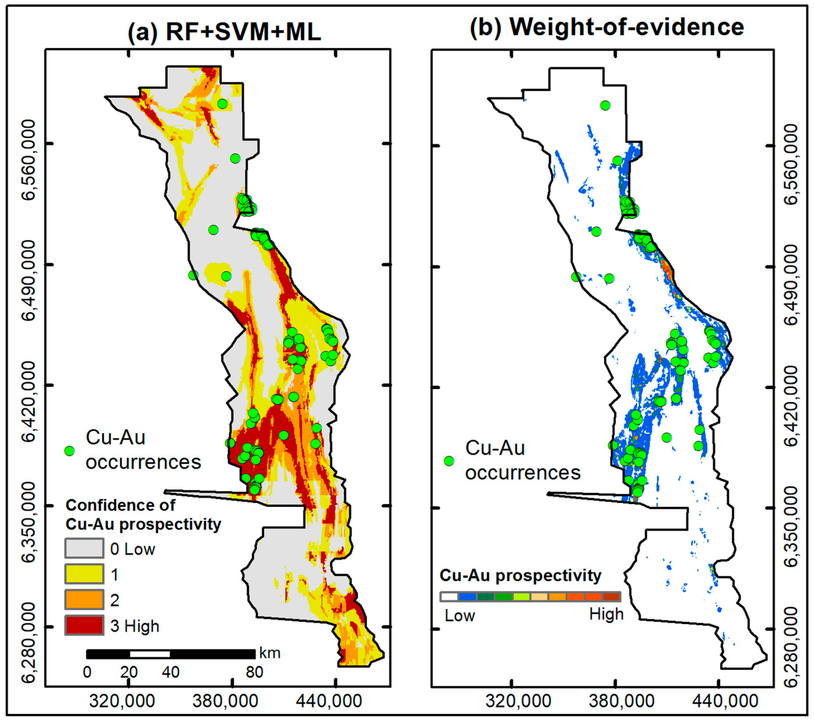
4. Results
5. Discussion
5.1. Interpretation and Comparison of Results with Existing Studies
5.2. Potential Future Work
6. Conclusions
Author Contributions
Funding
Data Availability Statement
Acknowledgments
Conflicts of Interest
References
- Marjoribanks, R. Geological Methods in Mineral Exploration and Mining; Springer: Berlin/Heidelberg, Germany, 2010. [Google Scholar]
- Zou, H.; Han, R.; Liu, M.; Cromie, P.; Zaw, K.; Fang, W.; Huang, J.; Ren, T.; Wu, J. Geological, geophysical, and geochemical characteristics of the Ban Kiouchep Cu–Pb–Ag deposit and its exploration significance in Northern Laos. Ore Geol. Rev. 2020, 124, 103603. [Google Scholar] [CrossRef]
- Ali, M.A.H.; Mewafy, F.M.; Qian, W.; Alshehri, F.; Ahmed, M.S.; Saleem, H.A. Integration of Electrical Resistivity Tomography and Induced Polarization for Characterization and Mapping of (Pb-Zn-Ag) Sulfide Deposits. Minerals 2023, 13, 986. [Google Scholar] [CrossRef]
- Porwal, A.K.; Kreuzer, O.P. Introduction to the special issue: Mineral prospectivity analysis and quantitative resource estimation. Ore Geol. Rev. 2010, 38, 121–127. [Google Scholar] [CrossRef]
- Hoover, D.B.; Klein, D.P.; Campbell, D.C.; du Bray, E. Geophysical methods in exploration and mineral environmental investigations. Prelim. Compil. Descr. Geoenviron. Miner. Depos. Models USGS Open-File Rep. 1995, 95, 19–27. [Google Scholar]
- Kearey, P.; Brooks, M.; Hill, I. An Introduction to Geophysical Exploration; Wiley-Blackwell: Maldan, MA, USA, 2002; Volume 4. [Google Scholar]
- Rose, A.W. Geochemical exploration. In Geochemistry. Encyclopedia of Earth Science; Springer: Dordrecht, The Netherlands, 1998. [Google Scholar]
- Grunsky, E.C.; Caritat, P.D. State-of-the-art analysis of geochemical data for mineral exploration. Geochemistry: Exploration, Environment. Analysis 2020, 20, 217–232. [Google Scholar]
- Agar, B.; Coulter, D. Remote sensing for mineral exploration—A decade perspective 1997–2007. In Proceedings of the Exploration 07: Fifth Decennial International Conference on Mineral Exploration, Toronto, ON, Canada, 9–12 September 2007; pp. 109–136. [Google Scholar]
- Sabins, F.F. Remote sensing for mineral exploration. Ore Geol. Rev. 1999, 14, 157–183. [Google Scholar] [CrossRef]
- Shirmard, H.; Farahbakhsh, E.; Müller, R.D.; Chandra, R. A review of machine learning in processing remote sensing data for mineral exploration. Remote Sens. Environ. 2022, 268, 112750. [Google Scholar] [CrossRef]
- Lawley, C.J.; Tschirhart, V.; Smith, J.W.; Pehrsson, S.J.; Schetselaar, E.M.; Schaeffer, A.J.; Houlé, M.G.; Eglington, B.M. Prospectivity modelling of Canadian magmatic Ni (±Cu±Co±PGE) sulphide mineral systems. Ore Geol. Rev. 2021, 132, 103985. [Google Scholar] [CrossRef]
- Harris, J.; Grunsky, E.; Behnia, P.; Corrigan, D. Data-and knowledge-driven mineral prospectivity maps for Canada’s North. Ore Geol. Rev. 2015, 71, 788–803. [Google Scholar] [CrossRef]
- Hosseini, S.A.; Abedi, M. Data envelopment analysis: A knowledge-driven method for mineral prospectivity mapping. Comput. Geosci. 2015, 82, 111–119. [Google Scholar] [CrossRef]
- Ma, Y.; Zhao, J.; Sui, Y.; Liao, S.; Zhang, Z. Application of knowledge-driven methods for mineral prospectivity mapping of polymetallic sulfide deposits in the southwest Indian ridge between 46° and 52° E. Minerals 2020, 10, 970. [Google Scholar] [CrossRef]
- Carranza, E.J.M.; Laborte, A.G. Data-driven predictive modeling of mineral prospectivity using random forests: A case study in Catanduanes Island (Philippines). Nat. Resour. Res. 2016, 25, 35–50. [Google Scholar] [CrossRef]
- Sun, T.; Li, H.; Wu, K.; Chen, F.; Zhu, Z.; Hu, Z. Data-driven predictive modelling of mineral prospectivity using machine learning and deep learning methods: A case study from southern Jiangxi Province, China. Minerals 2020, 10, 102. [Google Scholar] [CrossRef]
- Yousefi, M.; Nykänen, V. Data-driven logistic-based weighting of geochemical and geological evidence layers in mineral prospectivity mapping. J. Geochem. Explor. 2016, 164, 94–106. [Google Scholar] [CrossRef]
- Fu, C.; Chen, K.; Yang, Q.; Chen, J.; Wang, J.; Liu, J.; Xiang, Y.; Li, Y.; Rajesh, H. Mapping gold mineral prospectivity based on weights of evidence method in southeast Asmara, Eritrea. J. Afr. Earth Sci. 2021, 176, 104143. [Google Scholar] [CrossRef]
- Xiong, Y.; Zuo, R. GIS-based rare events logistic regression for mineral prospectivity mapping. Comput. Geosci. 2018, 111, 18–25. [Google Scholar] [CrossRef]
- Yuan, F.; Li, X.; Zhang, M.; Jowitt, S.M.; Jia, C.; Zheng, T.; Zhou, T. Three-dimensional weights of evidence-based prospectivity modeling: A case study of the Baixiangshan mining area, Ningwu Basin, Middle and Lower Yangtze Metallogenic Belt, China. J. Geochem. Explor. 2014, 145, 82–97. [Google Scholar] [CrossRef]
- Zeghouane, H.; Allek, K.; Kesraoui, M. GIS-based weights of evidence modeling applied to mineral prospectivity mapping of Sn-W and rare metals in Laouni area, Central Hoggar, Algeria. Arab. J. Geosci. 2016, 9, 373. [Google Scholar] [CrossRef]
- Brown, W.M.; Gedeon, T.; Groves, D.; Barnes, R. Artificial neural networks: A new method for mineral prospectivity mapping. Aust. J. Earth Sci. 2000, 47, 757–770. [Google Scholar] [CrossRef]
- Carranza, E.J.M.; Laborte, A.G. Random forest predictive modeling of mineral prospectivity with small number of prospects and data with missing values in Abra (Philippines). Comput. Geosci. 2015, 74, 60–70. [Google Scholar] [CrossRef]
- McKay, G.; Harris, J. Comparison of the data-driven random forests model and a knowledge-driven method for mineral prospectivity mapping: A case study for gold deposits around the Huritz Group and Nueltin Suite, Nunavut, Canada. Nat. Resour. Res. 2016, 25, 125–143. [Google Scholar] [CrossRef]
- Rodriguez-Galiano, V.; Sanchez-Castillo, M.; Chica-Olmo, M.; Chica-Rivas, M. Machine learning predictive models for mineral prospectivity: An evaluation of neural networks, random forest, regression trees and support vector machines. Ore Geol. Rev. 2015, 71, 804–818. [Google Scholar] [CrossRef]
- Zhang, N.; Zhou, K.; Li, D. Back-propagation neural network and support vector machines for gold mineral prospectivity mapping in the Hatu region, Xinjiang, China. Earth Sci. Inform. 2018, 11, 553–566. [Google Scholar] [CrossRef]
- Zuo, R. Geodata science-based mineral prospectivity mapping: A review. Nat. Resour. Res. 2020, 29, 3415–3424. [Google Scholar] [CrossRef]
- Zuo, R.; Carranza, E.J.M. Support vector machine: A tool for mapping mineral prospectivity. Comput. Geosci. 2011, 37, 1967–1975. [Google Scholar] [CrossRef]
- David, V. Cobar Deposits–Structural control. ASEG Ext. Abstr. 2018, 2018, 1–9. [Google Scholar] [CrossRef]
- Ford, A.; Peters, K.; Downes, P.; Blevin, P.; Greenfield, J.; Fitzherbert, J. Central Lachlan Orogen Mineral Systems Mineral Systems Report; Report GS2020/0741; Kenex Pty Ltd.: Dongara, WA, Australia, 2020. [Google Scholar]
- Folkes, C.B.; Carlton, A.; Eastlake, M.; Deyssing, L.; Trigg, S.; Montgomery, K.; Matthews, S.; Spampinato, G.; Roach, I.; Gilmore, P.; et al. The Cobar AEM Survey Interpretation Report; Report GS2021/1592; Mining, Exploration and Geoscience: Maitland, NSW, Australia, 2022. [Google Scholar]
- Glen, R.; Drummond, B.; Goleby, B.; Palmer, D.; Wake-Dyster, K. Structure of the Cobar Basin, New South Wales, based on seismic reflection profiling. Aust. J. Earth Sci. 1994, 41, 341–352. [Google Scholar] [CrossRef]
- Seccombe, P.K.; Jiang, Z.; Downes, P.M. Sulfur isotope and fluid inclusion geochemistry of metamorphic Cu–Au deposits, central Cobar area, NSW, Australia. Aust. J. Earth Sci. 2017, 64, 537–556. [Google Scholar] [CrossRef]
- Fitzherbert, J.A.; Downes, P.M. A Mineral System Model for Cu-Au-Pb-Zn-Ag Systems of the Cobar Basin, Central Lachlan Orogen, New South Wales 2020; Report GS2021/0042; Regional NSW: Maitland, NSW, Australia, 2020.
- Talebi, H.; Peeters, L.J.; Otto, A.; Tolosana-Delgado, R. A truly spatial Random Forests algorithm for geoscience data analysis and modelling. Math. Geosci. 2022, 54, 1–22. [Google Scholar] [CrossRef]
- Poudjom Djomani, Y.; Minty, B.R.S. Total Magnetic Intensity (TMI) Grid of Australia with Variable Reduction to Pole (VRTP) 2019, 7th ed.; Geoscience Australia: Canberra, Australia, 2019. [CrossRef]
- Poudjom Djomani, Y. Total Magnetic Intensity Grid of Australia 2019—First Vertical Derivative (1VD); Geoscience Australia: Canberra, Australia, 2019. [CrossRef]
- Lane, R.J.L.; Wynne, P.E.; Poudjom Djomani, Y.; Stratford, W.R.; Barretto, J.A.; Caratori Tontini, F. 2019 Australian National Gravity Grids: Free Air Anomaly, Complete Bouguer Anomaly, De-Trended Global Isostatic Residual, 400 m Cell Size (Includes Point Located Data); Geoscience Australia: Canberra, Australia, 2020.
- McCuaig, T.C.; Beresford, S.; Hronsky, J.M.A. Translating the mineral systems approach into an effective exploration targeting system. Ore Geol. Rev. 2010, 38, 128–138. [Google Scholar] [CrossRef]
- Occhipinti, S.; Metelka, V.; Lindsay, M.; Aitken, A.; Pirajno, F.; Tyler, I. The evolution from plate margin to intraplate mineral systems in the Capricorn Orogen, links to prospectivity. Ore Geol. Rev. 2020, 127, 103811. [Google Scholar] [CrossRef]
- Kirkby, A.; Musgrave, R.J.; Czarnota, K.; Doublier, M.P.; Duan, J.; Cayley, R.A.; Kyi, D. Lithospheric architecture of a Phanerozoic orogen from magnetotellurics: AusLAMP in the Tasmanides, southeast Australia. Tectonophysics 2020, 793, 228560. [Google Scholar] [CrossRef]
- Kirkby, A.L. Resistivity Model of the Southeast Australian Mainland from AusLAMP Magnetotelluric Data; Geoscience Australia: Canberra, Australia, 2020. [CrossRef]
- Kyi, D.; Duan, J.; Kirkby, A.L.; Stolz, N. Australian Lithospheric Architecture Magnetotelluric Project (AusLAMP): New South Wales: Data Release (Phase One). Record 2020/011; Geoscience Australia: Canberra, Australia, 2020. [CrossRef]
- Robertson, K.; Heinson, G.; Thiel, S. Lithospheric reworking at the Proterozoic–Phanerozoic transition of Australia imaged using AusLAMP Magnetotelluric data. Earth Planet. Sci. Lett. 2016, 452, 27–35. [Google Scholar] [CrossRef]
- Heinson, G.; Duan, J.; Kirkby, A.; Robertson, K.; Thiel, S.; Aivazpourporgou, S.; Soyer, W. Lower crustal resistivity signature of an orogenic gold system. Sci. Rep. 2021, 11, 15807. [Google Scholar] [CrossRef] [PubMed]
- Folkes, C.B.; Stuart, C. Fault Attribution for the Western Lachlan Orogen of NSW; Report GS2020/0955; Regional NSW: Maitland, NSW, Australia, 2020.
- Kennett, B.L.N.; Salmon, M.; Saygin, E.; Group, A.W. AusMoho: The variation of Moho depth in Australia. Geophys. J. Int. 2011, 187, 946–958. [Google Scholar] [CrossRef]
- Salmon, M.; Kennett, B.L.N.; Stern, T.; Aitken, A.R.A. The Moho in Australia and New Zealand. Tectonophysics 2013, 609, 288–298. [Google Scholar] [CrossRef]
- Stolz, E.; Spampinato, G.; Davidson, J. A statewide 3D geological model for New South Wales. ASEG Ext. Abstr. 2019, 2019, 1–4. [Google Scholar] [CrossRef]
- Biau, G.; Scornet, E. A random forest guided tour. Test 2016, 25, 197–227. [Google Scholar] [CrossRef]
- Ghosh, S.; Dasgupta, A.; Swetapadma, A. A Study on Support Vector Machine based Linear and Non-Linear Pattern Classification. In Proceedings of the 2019 International Conference on Intelligent Sustainable Systems (ICISS), Palladam, India, 21–22 February 2019; pp. 24–28. [Google Scholar]
- Singh, G.B.; Singh, G.B. Probabilistic Methods: Maximum Likelihood. In Fundamentals of Bioinformatics and Computational Biology: Methods and Exercises in MATLAB; Springer: Cham, Switzerland, 2015; pp. 273–286. [Google Scholar]


| Dataset | Source |
|---|---|
| Total Magnetic Intensity with variable reduction to the pole (VRTP) | Geoscience Australia https://ecat.ga.gov.au/geonetwork/srv/eng/catalog.search#/metadata/131519, accessed on 5 August 2021 |
| Total Magnetic Intensity–First Vertical Derivative (1VD) | Geoscience Australia https://ecat.ga.gov.au/geonetwork/srv/eng/catalog.search#/metadata/132275, accessed on 5 August 2021 |
| Gravity anomaly | Geoscience Australia https://ecat.ga.gov.au/geonetwork/srv/eng/catalog.search#/metadata/133023, accessed on 5 August 2021 |
| The Australian Lithospheric Architecture Magnetotelluric Project (AusLAMP) data | Geoscience Australia https://ecat.ga.gov.au/geonetwork/srv/eng/catalog.search#/metadata/131889, accessed on 20 August 2021 |
| Cobar AEM data | GSNSW and Geoscience Australia https://minview.geoscience.nsw.gov.au/#/(dlmodal:geophys-survey-air/AIR0759)?lon=148.5&lat=-32.5&z=7&bm=bm1&l=gp118:y:100, accessed on 30 July 2021 |
| Fault attribution of Zone 55W | GSNSW |
| AusMOHO | Australian Passive Seismic Server (AusPass) and the Australian National University Data Commons http://rses.anu.edu.au/seismology/AuSREM/AusMoho, accessed on 10 October 2021 |
| Depth to basement | GSNSW https://geonetwork.geoscience.nsw.gov.au/geonetwork/srv/eng/catalog.search#/metadata/97772139-31b0-412b-ab0a-86a6b2f66c2d, accessed on 20 August 2021 |
| Mineral Occurrence (NSW MetIndEx) data | GSNSW http://portal.auscope.org.au/geonetwork/srv/eng/catalog.search#/metadata/fd59b712f10394e68f07261981ac6d771d72aacd, accessed on 1 October 2021 |
| Pixel Value | Mineral Prospectivity | |||
|---|---|---|---|---|
| MapRandom_Forest | MapSVM | MAPMaxL | Final Map | |
| 0 | 0 | 0 | 0 | None |
| 1 | 0 | 0 | 1 | Low |
| 0 | 1 | 0 | 1 | |
| 0 | 0 | 1 | 1 | |
| 1 | 1 | 0 | 2 | Moderate |
| 0 | 1 | 1 | 2 | |
| 1 | 0 | 1 | 2 | |
| 1 | 1 | 1 | 3 | High |
Disclaimer/Publisher’s Note: The statements, opinions and data contained in all publications are solely those of the individual author(s) and contributor(s) and not of MDPI and/or the editor(s). MDPI and/or the editor(s) disclaim responsibility for any injury to people or property resulting from any ideas, methods, instructions or products referred to in the content. |
© 2023 by the authors. Licensee MDPI, Basel, Switzerland. This article is an open access article distributed under the terms and conditions of the Creative Commons Attribution (CC BY) license (https://creativecommons.org/licenses/by/4.0/).
Share and Cite
Senanayake, I.P.; Kiem, A.S.; Hancock, G.R.; Metelka, V.; Folkes, C.B.; Blevin, P.L.; Budd, A.R. A Spatial Data-Driven Approach for Mineral Prospectivity Mapping. Remote Sens. 2023, 15, 4074. https://doi.org/10.3390/rs15164074
Senanayake IP, Kiem AS, Hancock GR, Metelka V, Folkes CB, Blevin PL, Budd AR. A Spatial Data-Driven Approach for Mineral Prospectivity Mapping. Remote Sensing. 2023; 15(16):4074. https://doi.org/10.3390/rs15164074
Chicago/Turabian StyleSenanayake, Indishe P., Anthony S. Kiem, Gregory R. Hancock, Václav Metelka, Chris B. Folkes, Phillip L. Blevin, and Anthony R. Budd. 2023. "A Spatial Data-Driven Approach for Mineral Prospectivity Mapping" Remote Sensing 15, no. 16: 4074. https://doi.org/10.3390/rs15164074
APA StyleSenanayake, I. P., Kiem, A. S., Hancock, G. R., Metelka, V., Folkes, C. B., Blevin, P. L., & Budd, A. R. (2023). A Spatial Data-Driven Approach for Mineral Prospectivity Mapping. Remote Sensing, 15(16), 4074. https://doi.org/10.3390/rs15164074