RSS-LIWOM: Rotating Solid-State LiDAR for Robust LiDAR-Inertial-Wheel Odometry and Mapping

Abstract

Solid-state LiDAR offers multiple advantages over mechanism mechanical LiDAR, including higher durability, improved coverage ratio, and lower prices. However, solid-state LiDARs typically possess a narrow field of view, making them less suitable for odometry and mapping systems, especially for mobile autonomous systems. To address this issue, we propose a novel rotating solid-state LiDAR system that incorporates a servo motor to continuously rotate the solid-state LiDAR, expanding the horizontal field of view to 360°. Additionally, we propose a multi-sensor fusion odometry and mapping algorithm for our developed sensory system that integrates an IMU, wheel encoder, motor encoder and the LiDAR into an iterated Kalman filter to obtain a robust odometry estimation. Through comprehensive experiments, we demonstrate the effectiveness of our proposed approach in both outdoor open environments and narrow indoor environments.

1. Introduction

Odometry and mapping, also known as simultaneous localization and mapping (SLAM) [1], is an important task for autonomous mobile systems to localize themselves and interact with surroundings in unknown environments. RGB cameras and light detection and ranging (LiDAR) are two commonly used sensors for SLAM. RGB cameras capture detailed texture information of the environments, which offers useful constraints for visual SLAM [2,3,4,5,6]. However, they are easily affected by environmental lighting changes and lack depth information, which limits their effectiveness in 3D perception. LiDAR, as an active sensor, is less susceptible to environmental changes and provides accurate 3D information of the environment. Therefore, LiDAR-based SLAM has gained significant attention in applications where reliable perception is critical for ensuring safety and achieving high performance, such as autonomous driving [7,8] and specialized robotics.

Solid-state LiDAR sensors [9,10] have recently made remarkable progress and gained increasing attention for SLAM applications due to their numerous advantages over traditional mechanical LiDAR. Firstly, solid-state LiDAR eliminates the need for a mechanical rotating mechanism, making it more suitable for specialized environments with high/low temperatures and vibrations. Secondly, solid-state LiDAR is generally less expensive and more lightweight than mechanical LiDAR, making it more suitable for small mobile robots. Lastly, the most significant characteristic of solid-state LiDAR is its non-repeating scanning pattern, which results in significantly higher point-cloud density with increasing scan time compared to mechanism LiDAR.

However solid-state LiDAR typically has a narrower field of view (FOV) than mechanism LiDAR, e.g., Livox HAP with ${120}^{\circ }\times {25}^{\circ }$ FOV and HESAI FT120 with ${100}^{\circ }\times {75}^{\circ }$, which poses a challenge for scan registration. A narrow FOV represents that the robot struggles to obtain sufficient information from the environment, making the SLAM system vulnerable to less featured and elongated environments. Such a disadvantage is more severe for the mobile robot, where the sensor installation position is restricted and the installed height is commonly lower, resulting in less effective scanning information. Equipping multiple LiDARs can solve this problem, but it goes against the original intention of using more cost-effective solid-state LiDAR on mobile robots.

To address this challenge, we present a novel approach for solid-state LiDAR-based SLAM in mobile robot applications. The main contributions of our method are twofold:

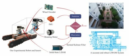
• We designed and implemented an economical rotating sensory platform that effectively expands the horizontal FOV of LiDAR to 360 degrees as shown in Figure 1.
• We propose a multi-source information fusion odometry system that combines the rotation encoding measurements of the rotating platform, IMU measurements, wheel speed odometry, and LiDAR odometry in an iterative extended Kalman filter to obtain robust and accurate pose estimation.

The proposed solution overcomes the limitations of solid-state LiDAR by providing a wider FOV while maintaining cost effectiveness. The multi-source information fusion algorithm ensures accurate and reliable localization, even in challenging environments where feature degradation may occur. Experimental results on outdoor, indoor and stair scenarios as shown in Figure 1c demonstrate the effectiveness and practicality of our proposed solution for mobile robot localization and mapping.

The remainder of this article is structured as follows: In Section 2, past relevant works are discussed. Section 3 provides the detailed design of the rotating platform and presents the kinematic model of our experimental mobile robot. Our proposed LiDAR odometry system is detailed in Section 4. In Section 5, we present the experimental results and evaluation. Finally, we conclude our work and discuss directions for future research in Section 6.

2. Related Work

Many existing approaches for LiDAR SLAM have been proposed. In this work, we mainly focus on the LiDAR-only odometry and mapping (LOM), LiDAR-IMU odometry and mapping (LIOM), and LiDAR-IMU-wheel odometry and mapping (LIWOM).

LiDAR-only odometry and mapping is based on the iterated closest points (ICP) [11,12,13,14,15] method, which was proposed by Besl et al. [11] for registering scans. ICP provides good results for dense 3D point clouds, but it requires exact point matching, which may not be available in sparse LiDAR measurements. To address this issue, Segal et al. [13] proposed a solution called Generalized-ICP, which is based on the distance between points and planes. Building upon this method, Zhang et al. [16] added point-to-edge matching and developed LOAM, a LiDAR odometry and mapping framework, in 2014. After that, many works have been proposed for LOAM, such as LeGO-LOAM [17], LOAM-Livox [18] and methods using semantic information [19,20], deep learning networks [21,22,23], or the most recent neural rendering techniques [24]. Current methods also allow loop closure detection and position correction by comparing the current frame with the keyframe [16,25] or combining with deep learning [20,26,27,28]. Further, there are methods using deep learning [29,30,31,32,33] to exclude dynamic objects in the environment and improve the accuracy of the LOAM system. However, due to their reliance only on LiDAR measurements, such methods may perform poorly in featureless environments. One solution to this issue is to fuse the measurements of other sensors, such as IMU, GNSS, camera and LiDAR measurements [34,35].

Combining LiDAR data with IMU measurements is one of the popular solutions to address the LiDAR SLAM degeneration problem in featureless environments [36]. Such methods can be divided into two groups, loosely coupled LiDAR-inertial odometry and mapping (LIOM) and tightly coupled LiDAR-inertial odometry. In the loosely coupled approaches, scan registration and data fusion are separated. For example, the method by Zhen et al. [37] first registers LiDAR scans and estimates robot poses, then fuses these estimates with IMU measurements. Another example is using IMU measurements as the initial estimate for registering LiDAR scans as presented in IMU-aided LOAM [16]. The loosely coupled approach has lower computational requirements but neglects the relationship between other states, such as the velocity and pose of new LiDAR measurements. In contrast, the tightly coupled LiDAR-inertial odometry directly combines the raw feature points of LiDAR with IMU measurements. Two main paths can be used for this approach, filter-based and optimization-based methods. For instance, Geneva et al. [38] fused IMU measurements and LiDAR plane feature points using graph optimization, while LIOM [25] also used graph optimization to fuse plane and edge features of IMU and LiDAR measurements. Gaussian particle filters [39] have also been used to fuse IMU and planar 2D-LiDAR. However, as the number of feature points and dimension of the system increase, the requirements for computational power quickly grow both in terms of graph optimization and Gaussian particle filter methods. Kalman filter and their variants, such as extended Kalman filter [40,41], adaptive Kalman filter [42,43], consensus Kalman filter [44] and iterated Kalman filter, have demonstrated more efficient and effective performance in real-time situations. Xu et al. [45,46] proposed the latest approaches, FAST-LIO and FAST-LIO2, that adopt the iterated extended Kalman filter in the LIOM field. Bai et al. [47,48] also increased the speed of integrating the LIOM system by replacing the ikd-tree with iVox.

In complex real-world environments, enhancing perception-based odometry methods by integrating the robot’s kinematics model obtained from sensors such as wheel encoders can improve the robustness of the odometry and mapping results. In the field of visual SLAM, there are instances where wheel encoder messages have been incorporated into existing odometry and mapping frameworks. For example, Zhang et al. [5] employed an iterative optimization method based on sliding windows to fuse visual, IMU, and wheel encoder measurements. Liu et al. [5] adopted a tightly coupled approach, integrating wheel encoder and IMU measurements during a pre-integration stage. However, the utilization of both LiDAR and wheel encoders is relatively limited. Júnior et al. [49] proposed an approach that combines LiDAR measurements, IMU data, and wheel encoder information to establish an odometry and mapping framework specifically designed for challenging environments. Yuan et al. [50] introduced a framework based on bundle adjustment (BA) to achieve similar functionality. Existing methods mainly focus on fixed LiDAR sensors and perform poorly when directly applied with rotating LiDAR sensors due to the special motion characteristics.

To bridge this gap, we propose a tightly coupled method to fuse rotating LiDAR data with IMU and wheel encoder measurements to obtain an accurate odometry and dense mapping result. During the motion compensation stage for rotating solid-state LiDAR scans, we combine IMU measurements with motor encoder readings to generate undistorted point clouds. We install this solid-state LiDAR on a rotating platform and run our approach on a track robot designed by our lab. We test our odometry and mapping approach for rotating solid-state LiDAR in complex environments. To the best of our knowledge, our approach is the first work that combines the rotating ability of solid-state LiDARs with exclusive odometry and mapping frameworks for multiple complex environment SLAM tasks.

3. Rotating Sensory Platform and Experimental Robot

3.1. Experimental Platforms

We first introduce our designed rotating sensory platform for solid-state LiDAR. As shown in Figure 1a, we use the Livox HAP solid-state LiDAR sensor, which provides a horizontal FOV of 120° and vertical FOV of 25°. Note that our rotating platform is not limited to this type of LiDAR, and theoretically it can work with any type of LiDAR. Our rotating platform uses a servo motor to continuously rotate around the z-axis, expanding the horizontal FOV of LiDAR to 360°. We use conductive slip rings to achieve data transmission during the rotation process. In this paper, we set the motor speed to 3000 rotations per minute (RPM) with a reduction ratio of 100, thus resulting in a speed of 30 RPM for the solid-state LiDAR. We visualize the point cloud obtained by the LiDAR sensor in a stationary state for 0.1 s (see Figure 2a), 2 s (see Figure 2b), and on our rotating platform for 2 s (see Figure 2c). As can be seen in Figure 2a,b, benefiting from the non-repeating scanning characteristic of the solid-state LiDAR, a longer scanning period results in higher coverage of the scene. Comparing Figure 2b,c, we can see that using our rotating platform, the point cloud collected by the LiDAR can cover greater areas of the scene.

We use our designed tracked robot for evaluating the proposed odometry and mapping experiment in complex campus environments. Figure 1b shows the robot equipped with our rotating sensory platform. The size of the rotating platform is $30\mathrm{cm}\times 16\mathrm{cm}\times 27\mathrm{cm}$, and when installed on the robot, the height of the LiDAR optical center from the ground is 40 cm. The robot is equipped with four independently driven fins with strong obstacle-crossing abilities, allowing us to conduct experiments in more complex terrains, such as indoor environments with steps, even multi-floor stairs. The robot also equips a wheel encoder, enabling us to form its kinematic equation as

$$\left[\begin{array}{c}{v}_x\\ {\omega }_{yaw}\end{array}\right]=\left[\begin{array}{cc}\frac{1}{2}& \frac{1}{2}\\ \frac{L}{2}& -\frac{L}{2}\end{array}\right]\left[\begin{array}{c}{v}_L\\ v_R\end{array}\right],$$

(1)

where $v_R$ and $v_L$ are the velocity of the left and right of the main track, and L is the distance of the two main track centers. The final measurement of the wheel encoder can be written as ${\mathit{v}}_O=\left[v_{x}00\right]$ and ${\mathit{\omega }}_O=\left[00{\omega }_{yaw}\right]$.

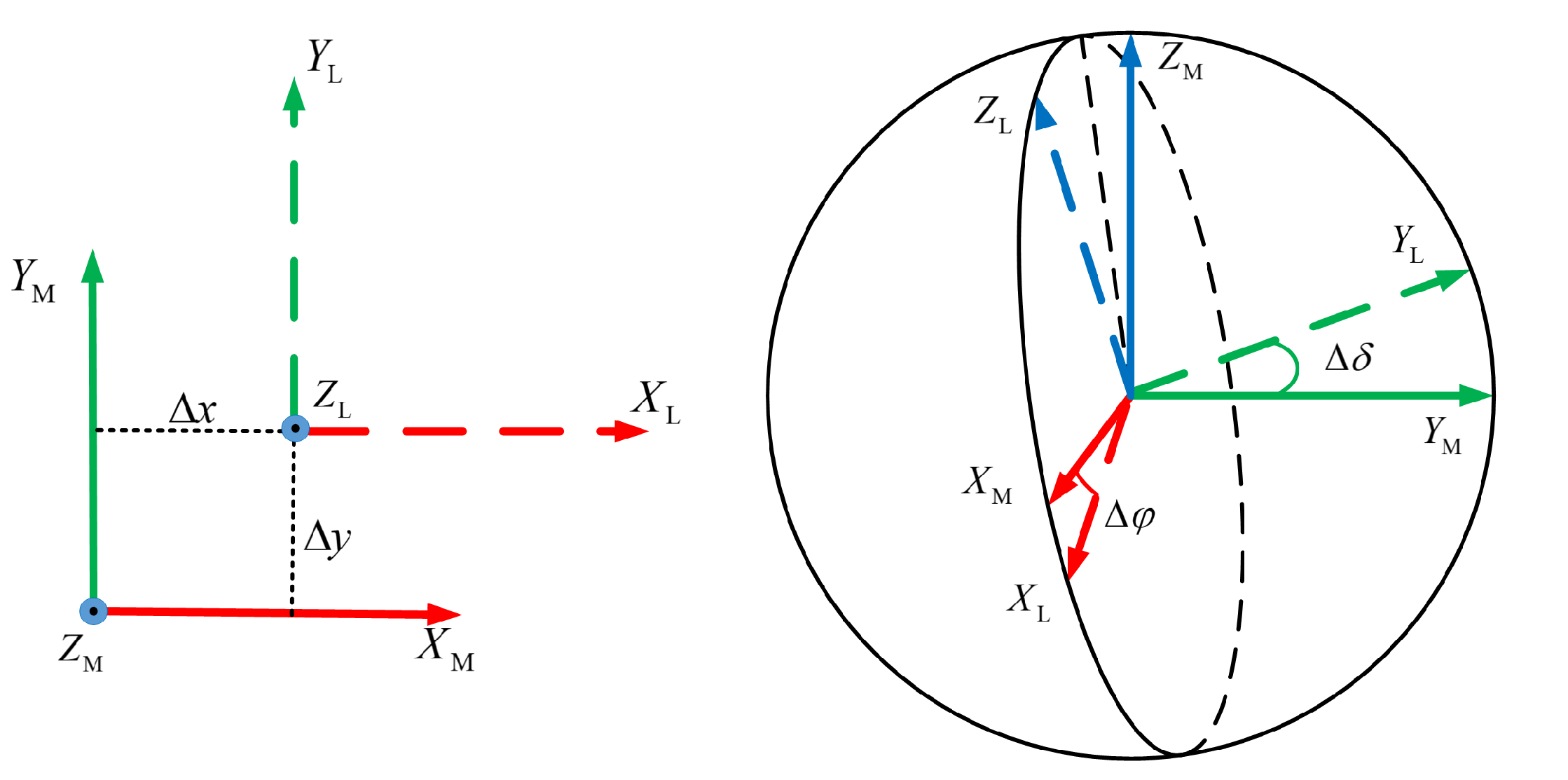
3.2. Extrinsic Calibration

In this section, we introduce the extrinsic calibration process of our sensor system. Some notations used in this paper are shown in

Table 1. Notations in our paper.

Symbols	Meaning
$T{s}_k^A$	The timestamp of the k-th measurements of senor A.
${\mathcal{S}}_n^A,{}^d{\mathcal{S}}_n^A$	scan and after downsampling in A frame.
${\tilde{\mathit{x}}}^A,{\widehat{\mathit{x}}}^A,\delta {\mathit{x}}^A$	true state variables, nominal state variables and error state variables calculated by measurement of senor A.
${}^A{\mathbf{T}}_B,{}^A{\mathbf{R}}_B,{}^A{\mathbf{t}}_B$	T is transform from B to A that R is rotation and t is translation.
${(·)}_W,{(·)}_I,{(·)}_L,{(·)}_O,{(·)}_M$	The coordinate system of world, IMU, LiDAR, wheel odometry and rotating platform.

. The definition of the sensor coordinate systems of our experimental robot is given in Figure 1. We also define the coordinate system of the LiDAR, IMU and robot such that the coordinate origin of the LiDAR coincides with the optical center, with the X-axis pointing towards the scanning direction, and the coordinate system of the IMU coincides with that of the accelerometer. The coordinate origin of the robot is located at the center of gravity of the robot. For the coordinate system of the rotating platform, we define the z-axis pointing upward as coinciding with the rotating axis, and the x-axis and y-axis coincide with that of the robot.The center is defined at the same height as the LiDAR optical center for convenience. Ideally, the rotating axis of the rotating platform should coincide with the z-axis of the LiDAR. However, mechanical installation issues can cause errors in both the distance from the LiDAR center to the rotating axis and the angle between these two axes as in Figure 3. Therefore, we need to calibrate the rotating platform with the LiDAR sensor. We denote the extrinsic parameters between the LiDAR system and the rotating platform system as ${}^M{\mathbf{T}}_L$ 

$$\begin{array}{cc}\hfill {}^M{\mathbf{R}}_L& =\left[\begin{array}{ccc}cos(\Delta \phi )& 0& sin(\Delta \phi )\\ sin(\Delta \phi )sin(\Delta \delta )& cos(\Delta \delta )& -cos(\Delta \phi )sin(\Delta \delta )\\ -sin(\Delta \phi )cos(\Delta \delta )& sin(\Delta \delta )& cos(\Delta \phi )cos(\Delta \delta )\end{array}\right],\hfill \end{array}$$

(2)

$$\begin{array}{cc}\hfill {}^M{\mathbf{t}}_L& =\left[\begin{array}{c}\Delta x\\ \Delta y\\ 0\end{array}\right],\hfill \end{array}$$

(3)

$$\begin{array}{cc}\hfill {}^M{\mathbf{T}}_L& =\left[\begin{array}{cc}{}^M{\mathbf{R}}_L& {}^M{\mathbf{t}}_L\\ 0& 1\end{array}\right].\hfill \end{array}$$

(4)

where $[\Delta x,\Delta y]$ are the translation parameters and $[\Delta \phi ,\Delta \delta ]$ are the rotating parameters represented in the Euler angles, i.e., the roll and pitch angle. We design an extrinsic calibration for our platform to obtain the extrinsic parameters ${}^M{\mathbf{T}}_L$ as follows.

We firstly collect scans at different rotating angles ${\theta }_n$ of the platform and can obtain a related transform as Equation (5)

$$\begin{array}{cc}\hfill {\mathbf{R}}_{{\theta }_n}& =\left[\begin{array}{ccc}cos\left({\theta }_n\right)& -sin\left({\theta }_n\right)& 0\\ sin\left({\theta }_n\right)& cos\left({\theta }_n\right)& 0\\ 0& 0& 1\end{array}\right].\hfill \end{array}$$

(5)

Each angle is related to a LiDAR pose measurement ${\mathbf{T}}_n=\mathbf{T}\left({\theta }_n\right){}^M{\mathbf{T}}_L$ in the world frame, which is defined as coinciding with the original rotating platform frame. For each pair of angles $\{{\theta }_i,{\theta }_j\}$, we can establish the relative pose measurement from ${\theta }_i$ to ${\theta }_j$ as ${}^{{\theta }_i}{\mathbf{T}}_{\theta j}$:

$$\begin{array}{cc}\hfill \mathbf{T}\left({\theta }_n\right)& =\left[\begin{array}{cc}{\mathbf{R}}_{{\theta }_n}& 0\\ 0& 1\end{array}\right],\hfill \end{array}$$

(6)

$$\begin{array}{cc}\hfill {}^{{\theta }_i}{\mathbf{T}}_{\theta j}& ={\left(\mathbf{T}\left({\theta }_i\right){}^M{\mathbf{T}}_L\right)}^{-1}\mathbf{T}\left({\theta }_j\right){}^M{\mathbf{T}}_L={{}^M{\mathbf{T}}_L}^{-1}\mathbf{T}({\theta }_i-{\theta }_j){}^M{\mathbf{T}}_L,\hfill \end{array}$$

(7)

By obtaining the relative pose observation ${}^{{\theta }_i}{\mathbf{T}}_{\theta j}^{\prime }$ using point cloud registration, we can then establish the optimization function as

$$\begin{array}{cc}\hfill & \underset{{}^M{\mathbf{T}}_L}{min}\sum _{j=1}^N\sum _{i=1}^N{\parallel {}^{{\theta }_i}{\mathbf{T}}_{\theta j}^{\prime }-{}^{{\theta }_i}{\mathbf{T}}_{\theta j}\parallel }_F(i\ne j)\hfill \end{array}$$

(8)

$$\begin{array}{cc}\hfill =& \underset{{}^M{\mathbf{T}}_L}{min}\sum _{j=1}^N\sum _{i=1}^N{\parallel ({}^{{\theta }_i}{\mathbf{T}}_{\theta j}^{\prime }-{{}^M{\mathbf{T}}_L}^{-1}T({\theta }_i-{\theta }_j){}^M{\mathbf{T}}_L)\parallel }_F(i\ne j).\hfill \end{array}$$

(9)

which can be solved iteratively using the Levenberg–Marquardt algorithm.

To obtain precise observation of relative pose ${}^{{\theta }_i}{\mathbf{T}}_{\theta j}^{\prime }$, we perform the extrinsic calibration in a structured environment, and obtain the ground truth dense point cloud of the environment using a Faro FocusS350 scanner. FocusS350 is a high-precision laser scanner with a measuring range of up to 350 m and a measurement accuracy of 1 mm (Figure 4).

For each rotating angle, we keep the platform stationary and collect all the point clouds acquired by the LiDAR within 5 s as one scan. Each scan is registered to the ground truth point cloud of the environment using ICP [11] to solve the precise pose ${\mathbf{T}}_{{\theta }_i}^{\prime }$ in the Faro frame. The relative pose observation is then obtained as ${}^{{\theta }_i}{\mathbf{T}}_{\theta j}$. As the registration is performed between the sparse scan and the ground truth dense point clouds, we can obtain the relative transformation between the sparse scans even without overlap to include more constraints in the optimization function Equation (9) to obtain a better calibration result.

For the extrinsic parameters between the wheel odometry and the IMU ${}^I{\mathbf{T}}_O$, we use the calibration method described in [6]. For the extrinsic parameters between the rotating platform and the IMU ${}^I{\mathbf{T}}_M$, we opt for an indirect method. We fix the rotating platform and adopt the LiDAR-IMU calibration method described in [51] to calculate the transformation between the LiDAR frame and IMU frame ${}^I{\mathbf{T}}_L$, and then calculate the extrinsic parameters as ${}^I{\mathbf{T}}_M={}^I{\mathbf{T}}_L{}^L{\mathbf{T}}_M$.

4. LiDAR-Inertial-Wheel Odometry and Mapping

4.1. System Overview

The overview of our approach is presented in Figure 5. The measurements of the IMU, motor encoder, wheel encoder and LiDAR are fed into our state estimation module for a fast state estimation. The estimated pose is then used to register the point cloud with the built global map. The updated map is finally used for registration in the next step.

4.2. State Estimation

We first model the state of our system as $x=\left[p\theta v{b}_a{b}_{\omega }g\right]$, where p is the pose, v is the velocity, $\theta$ is the Euler angle, $b_a$ is the bias of the accelerometer, $b_{\omega }$ is the bias of the gyroscope, and g is gravity. We use the iterated Kalman filter as the optimization framework. Instead of directly updating the state in a general Kalman filter, the iterated Kalman filter updates the errors of the state, i.e., $\delta \mathit{x}=\tilde{\mathit{x}}-\widehat{\mathit{x}}$, where $\widehat{\mathit{x}}$ is the nominal state and $\tilde{\mathit{x}}$ is the true state. This allows for a smoother and more stable state estimation. The iterated Kalman filter optimizes the estimation of $\delta \mathit{x}$ and incorporates it into the nominal state variables $\widehat{\mathit{x}}$ to obtain the final state estimation.

4.2.1. IMU Integration

In the IMU integration stage, we use IMU measurements as inputs to predict the state estimation:

$$\begin{array}{cc}\hfill {\widehat{\mathit{x}}}_{n+1}^I& ={\widehat{\mathit{x}}}_n^I+\Delta tf({\widehat{\mathit{x}}}_n^I,\mathit{u},0),\hfill \end{array}$$

(10)

where $f({\widehat{\mathit{x}}}_n^I,\mathit{u},0)={\dot{\widehat{\mathit{x}}}}_n^I$ is the state equation of ${\widehat{x}}_n^I$ in continuous time with noise w set to 0, and $\Delta t=T{s}_{n+1}^I-T{s}_n^I$ refers to the time interval between consecutive IMU time steps $T{s}_{n+1}^I$ and $T{s}_n^I$.

We follow [41] and calculate $\delta {\mathit{x}}_{n+1}^I$ as

$$\begin{array}{cc}\hfill \delta {\mathit{x}}_{n+1}^I& ={\mathbf{F}}_n\delta {\mathit{x}}_n^I+{\mathbf{G}}_{n}w,\hfill \end{array}$$

(11)

$$\begin{array}{cc}\hfill {\mathbf{F}}_n& ={\left[\begin{array}{cccccc}{\mathbf{I}}_{3\times 3}& 0& {\mathbf{I}}_{3\times 3}\Delta t& 0& 0& 0\\ 0& {\mathbf{I}}_{3\times 3}+{\lfloor \mathit{\omega }-{\mathit{b}}_{\omega }\rfloor }_{\times }& 0& 0& -{\mathbf{I}}_{3\times 3}\Delta t& 0\\ 0& -{\mathbf{R}}_n{\lfloor \mathit{a}-{\mathit{b}}_a\rfloor }_{\times }\Delta t& {\mathbf{I}}_{3\times 3}& -{\mathbf{R}}_n\Delta t& 0& {\mathbf{I}}_{3\times 3}\Delta t\\ 0& 0& 0& {\mathbf{I}}_{3\times 3}& 0& 0\\ 0& 0& 0& 0& {\mathbf{I}}_{3\times 3}& 0\\ 0& 0& 0& 0& 0& {\mathbf{I}}_{3\times 3}\end{array}\right]}_{18\times 18},\hfill \end{array}$$

(12)

$$\begin{array}{cc}\hfill {\mathbf{G}}_n& ={\left[\begin{array}{cccc}0& 0& 0& 0\\ 0& -{\mathbf{I}}_{3\times 3}& 0& 0\\ -{\mathbf{R}}_n& 0& 0& 0\\ 0& 0& {\mathbf{I}}_{3\times 3}& 0\\ 0& 0& 0& {\mathbf{I}}_{3\times 3}\\ 0& 0& 0& 0\end{array}\right]}_{18\times 12},\hfill \end{array}$$

(13)

where ${\mathit{u}}^{\top }={\left[\omega a\right]}^{\top }$ is the measurements of the gyrometer and accelerometer of IMU, and $\mathit{w}={\left[{\mathit{a}}_n^{\top }{\mathit{\omega }}_n^{\top }{\mathit{a}}_w^{\top }{\mathit{\omega }}_w^{\top }\right]}^{\top }$ refers to the Gaussian noise of the gyrometer and accelerometer, and the bias of the gyrometer and accelerometer, respectively. ${\lfloor ·\rfloor }_{\times }\in {\mathcal{R}}_{3\times 3}$ represents transferring the 3D vector to its skew–symmetric matrix. ${\mathbf{I}}_{3\times 3}$ is the $3\times 3$ identity matrix, and ${\mathbf{R}}_n$ is the transformation from the world frame to the IMU frame. ${\mathit{b}}_a$ and ${\mathit{b}}_{\omega }$ are the bias of the gyrometer and accelerometer.

Using ${\mathbf{F}}_n$ and ${\mathbf{G}}_n$, we can then propagate the covariance ${\mathbf{P}}_n$ of state $x_n$ iteratively as the following:

$$\begin{array}{cc}\hfill {\widehat{\mathbf{P}}}_{n+1}^I& ={\mathbf{F}}_n{\widehat{\mathbf{P}}}_n^I{\mathbf{F}}_n^{\top }+({\mathbf{G}}_n\Delta t)\mathbf{Q}{({\mathbf{G}}_n\Delta t)}^{\top },\hfill \end{array}$$

(14)

where $\mathbf{Q}\in {\mathcal{R}}_{12\times 12}$ represents the covariance of noise w.

4.2.2. Wheel Encoder Residual Computation and State Update

After the IMU integration, we obtain the state estimation ${\widehat{\mathit{x}}}_{n+1}^I$ and the covariance matrix ${\widehat{\mathbf{P}}}_{n+1}^I$ at iteration $n+1$. In the low-velocity situation, the cumulative error of the IMU accelerometer can greatly affect the velocity estimation. To eliminate this error $\delta v$ in $\delta \mathit{x}$ and achieve a more stable velocity estimation, we build the observation model to rectify velocity estimation ${\widehat{v}}_{n+1}$ in the propagated state ${\widehat{\mathit{x}}}_{n+1}$ based on the measurements from the wheel encoder:

$$\begin{array}{cc}\hfill & {\mathbf{h}}_W\left(\mathit{x}\right)=({}^I{\mathbf{R}}_O^{\top }{\mathit{v}}_O+{}^I{\mathbf{t}}_O\times {\mathit{\omega }}_O)-{}^I{\mathbf{R}}_W^{\top }{\widehat{\mathit{v}}}_{n+1}^I,\hfill \end{array}$$

(15)

where ${\mathit{v}}_{xO}$ is the measurement of the wheel encoder calculated as in Equation (1), and ${}^O{\mathbf{R}}_I$ and ${}^O{\mathbf{t}}_I$ are the extrinsic parameters between the wheel encoder with IMU, and ${}^W{\mathbf{R}}_I$ is the extrinsic parameters between the world frame with IMU. Based on the observation model, we can then formulate the optimization function as

$$\begin{array}{cc}\hfill & \underset{\delta \mathit{x}}{min}{\parallel \delta \mathit{x}\parallel }_{{{\widehat{\mathbf{P}}}_{n+1}}^{-1}}+{\parallel {\mathbf{h}}_O\left(\mathit{x}\right)+{\mathbf{J}}_{h_O}\delta \mathit{x}\parallel }_{{\mathbf{M}}_O^{-1}},\hfill \end{array}$$

(16)

where ${\mathbf{M}}_O^{-1}$ is the noise of the wheel encoder measurements, and ${\mathbf{J}}_{h_O}$ is the Jacobian w.r.t. velocity v in state variables x. Equation (16) can be solved by the Kalman filter as follows:

$$\begin{array}{cc}\hfill {\mathbf{K}}^O& ={\widehat{\mathbf{P}}}_{n+1}^I{\mathbf{H}}_O^{\top }{({\mathbf{H}}_O{\widehat{\mathbf{P}}}_{n+1}^I{\mathbf{H}}_O^{\top }+{\mathbf{M}}_O)}^{-1},\hfill \end{array}$$

(17)

$$\begin{array}{cc}\hfill \delta {\mathit{x}}_{n+1}^O& ={\mathbf{H}}_O\delta {\mathit{x}}_{n+1}^I-{\mathbf{h}}_O({\widehat{\mathit{x}}}_{n+1}^I+\delta {\mathit{x}}_{n+1}^I)\hfill \end{array}$$

(18)

$$\begin{array}{cc}\hfill {\widehat{\mathit{x}}}_{n+1}^O& ={\widehat{\mathit{x}}}_{n+1}^I+{\mathbf{K}}^O\delta {\mathit{x}}_{n+1}^O,\hfill \end{array}$$

(19)

$$\begin{array}{cc}\hfill {\widehat{\mathbf{P}}}_{n+1}^O& =(\mathbf{I}-{\mathbf{K}}^O{\mathbf{H}}_O){\widehat{\mathbf{P}}}_{n+1}^I,\hfill \end{array}$$

(20)

where the Kalman gain ${\mathbf{K}}^O$ is solved in Equation (17), $\delta x_{n+1}^O$ is Equation (18), and used to update state ${\widehat{x}}_{n+1}^O$ in Equation (19) and covariance ${\widehat{\mathbf{P}}}_{n+1}^O$ in Equation (20).

The updated ${\widehat{x}}_{n+1}^O$ and ${\widehat{\mathbf{P}}}_{n+1}^O$ will be then used for motion compensation and the next optimization of the state.

4.2.3. Motion Compensation

In order to address the distortions and deviations caused by the movement of the robot and the rotation of the motor in the LiDAR scanning results, a kinematic analysis is performed. This analysis aims to compensate for the motion effects and determine the position of all points at the end of the scanning in the IMU frame system. The kinematic analysis assumes a constant velocity and utilizes the transformation information obtained from the extrinsic calibration process.

The first step in motion compensation involves establishing a motion model for each point within a single scanning by transforming the points from the LiDAR frame to the world frame as

$$\begin{array}{cc}\hfill {}^W\mathit{p}& ={}^W{\mathbf{R}}_I({}^I{\mathbf{R}}_L{}^L\mathit{p}+{}^I{\mathbf{t}}_L)+{}^W{\mathbf{t}}_I.\hfill \end{array}$$

(21)

The kinematic relationship between the velocities ${}^W\dot{\mathit{p}}$ and ${}^L\dot{\mathit{p}}$ can be derived as

$$\begin{array}{cc}\hfill {}^W\dot{\mathit{p}}& ={}^W{\dot{\mathbf{R}}}_I({}^I{\mathbf{R}}_L{}^L\mathit{p}+{}^I{\mathbf{t}}_L)+{}^W{\mathbf{R}}_I({}^I{\dot{\mathbf{R}}}_L{}^L\mathit{p}+{}^I{\mathbf{R}}_L{}^L\dot{\mathit{p}}+{}^I{\dot{\mathbf{t}}}_L)+{}^W{\dot{\mathbf{t}}}_I,\hfill \end{array}$$

(22)

where ${}^I{\mathbf{R}}_L={}^I{\mathbf{R}}_M{\mathbf{R}}_{{\theta }_i}{}^M{\mathbf{R}}_L$ and ${}^I{\mathbf{t}}_L={}^I{\mathbf{R}}_M{\mathbf{R}}_{{\theta }_i}{}^M{\mathbf{t}}_L+{}^I{\mathbf{t}}_M$ are the transformations from LiDAR frame to IMU frame. Assuming that the environment is perfectly stationary, i.e., ${}^W\dot{\mathit{p}}=0$, we can further derive Equation (22) to solve the velocity of the point in LiDAR frame as

$$\begin{array}{}\mathrm{(23)}& \hfill {}^L\dot{\mathit{p}}& =-{}^I{\mathbf{R}}_L^{\top }{}^W{\mathbf{R}}_I^{\top }{}^W{\dot{\mathbf{R}}}_I{}^I{\mathbf{R}}_L{}^L\mathit{p}-{}^I{\mathbf{R}}_L^{\top }{}^W{\mathbf{R}}_I^{\top }{}^W{\dot{\mathbf{R}}}_I{}^I{\mathbf{t}}_L-{}^I{\mathbf{R}}_L^{\top }{}^W{\mathbf{R}}_I^{\top }{}^W{\dot{\mathbf{t}}}_I-{}^I{\mathbf{R}}_L^{\top }{}^I{\dot{\mathbf{t}}}_L-{}^I{\mathbf{R}}_L^{\top }{}^I{\dot{\mathbf{R}}}_L^{\top }{}^L\mathit{p},\hfill & \hfill & =-{}^M{\mathbf{R}}_L^{\top }{\mathbf{R}}_{{\theta }_i}^{\top }{}^I{\mathbf{R}}_M^{\top }{\lfloor {\omega }_I\rfloor }_{\times }{}^I{\mathbf{R}}_M{\mathbf{R}}_{{\theta }_i}{}^M{\mathbf{R}}_L{}^L\mathit{p}-{}^M{\mathbf{R}}_L^{\top }{\mathbf{R}}_{{\theta }_i}^{\top }{}^I{\mathbf{R}}_M^{\top }{\lfloor {\omega }_I\rfloor }_{\times }({}^I{\mathbf{R}}_M{\mathbf{R}}_{{\theta }_i}{}^M{\mathbf{t}}_L+{}^I{\mathbf{t}}_M)\hfill \mathrm{(24)}& \hfill & -{}^M{\mathbf{R}}_L^{\top }{\mathbf{R}}_{{\theta }_i}^{\top }{}^I{\mathbf{R}}_M^{\top }{}^W{\mathbf{R}}_I^{\top }{}^W{\dot{\mathbf{t}}}_I-{}^M{\mathbf{R}}_L^T{\mathbf{R}}_{{\theta }_i}^{\top }{}^I{\mathbf{R}}_M^{\top }{}^I{\mathbf{R}}_M{\mathbf{R}}_{{\theta }_i}{\lfloor {\omega }_M\rfloor }_{\times }{}^M{\mathbf{t}}_L-{\lfloor {\omega }_M\rfloor }_{\times }{}^L\mathit{p},\hfill \end{array}$$

where ${\mathit{\omega }}_I$ is the measurements of the IMU gyrometer, and ${\mathit{\omega }}_M$ is the reading of the motor encoder, and ${}^W{\dot{\mathbf{t}}}_I$ is the velocity of the robot in the real world, which can be obtained by state optimization. Using the timestamp of each point ${}^L{\mathit{p}}_i^k$ in a single scan, we can then compensate for the motion distortion for each point by projecting it to the end of the scan as

$${}^L{\mathit{p}}_i^{k-end}={}^L{\mathit{p}}_i^k+{}^L\dot{\mathit{p}}(1-{ϵ}_i)\Delta t,$$

(25)

where ${ϵ}_i=\left(t_i^L-T{s}_k^L\right)/\left(T{s}_k^L-T{s}_{k-1}^L\right)$ is the scanning time duration of the k-th scan, $\Delta t=T{s}_k^L-T{s}_{k-1}^L$, and $t_i^L$ is the timestamp of point ${}^L{\mathit{p}}_i^k$.

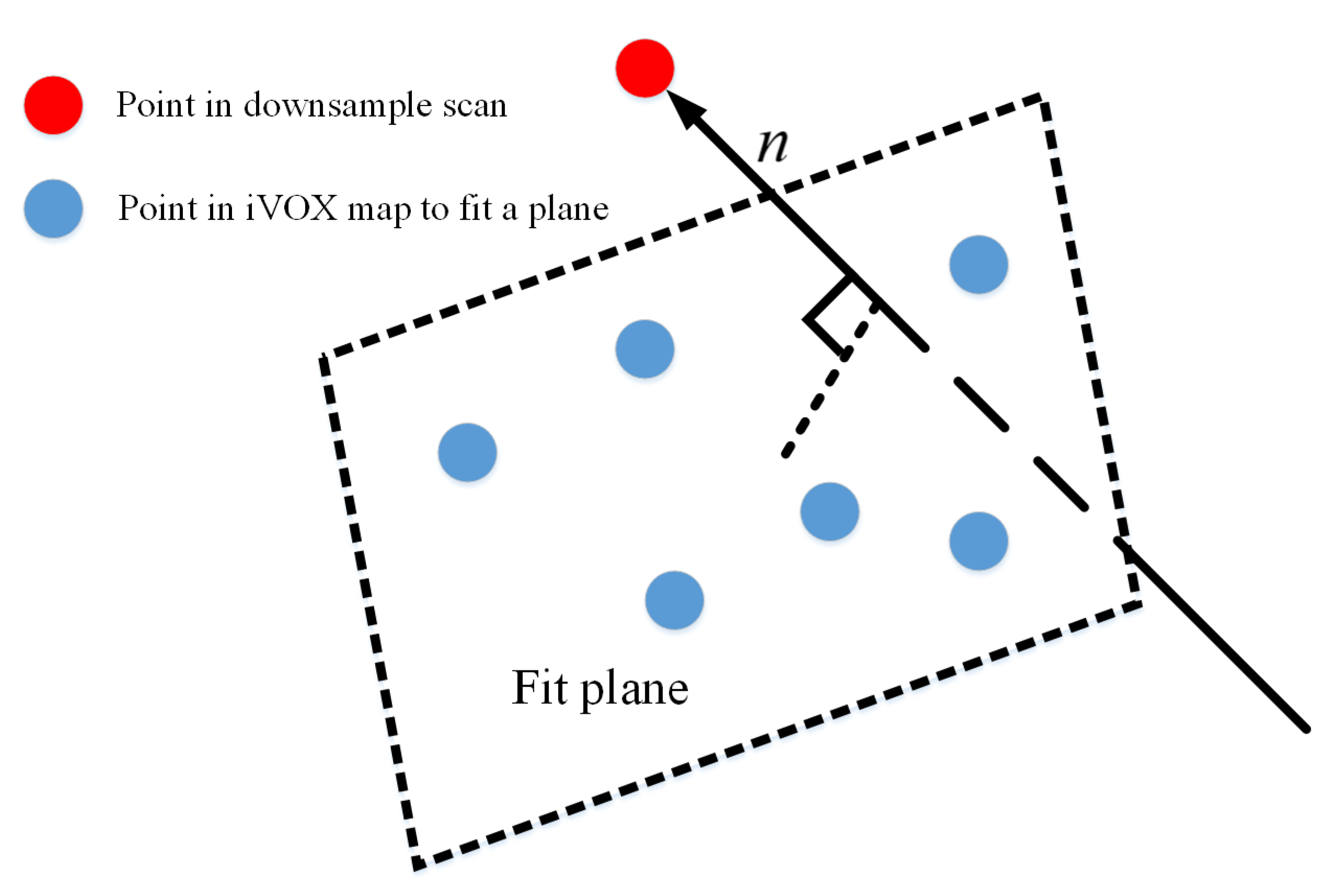
4.2.4. Point Cloud Residual Computation and State Update

After the motion compensation, we obtain the undistorted point cloud denoted as ${\mathcal{S}}_n^L$ and use it to construct the residual. Assuming that the current iteration of the iterated Kalman filter is $n+1$, and the corresponding state estimation is ${\widehat{x}}_{n+1}^O$ and the covariance matrix is ${\widehat{\mathbf{P}}}_{n+1}^O$. When the new scan ${\mathcal{S}}_n^L$ is input, a downsample process will be executed that generates ${}^d{\mathcal{S}}_n^L$. Then, we transform the point cloud ${}^d{\mathcal{S}}_n^L$ into the world frame as

$$\begin{array}{c}\hfill {}^d{\mathcal{S}}_n^W={}^W{\mathbf{T}}_I{}^I{\mathbf{T}}_L{}^d{\mathcal{S}}_n^L.\end{array}$$

(26)

After downsampling and transforming, the nearest points of ${}^d{\mathcal{S}}_n^W$ in the hash map are retrieved. Each set of the nearest points is used to fit a plane and calculate the distance between the plane with the corresponding point in the downsampled point cloud, as shown in Figure 6.

Specifically, for each point ${\mathit{p}}_j(x_j,y_j,z_j)\in {}^d{\mathcal{S}}_n^W$, we find its nearest points set $\mathbf{A}$ in the built map:

$$\begin{array}{cc}\hfill \mathbf{A}& ={[{\mathit{q}}_1{\mathit{q}}_2\dots {\mathit{q}}_i]}_{i\times 3}.\hfill \end{array}$$

(27)

We then calculate the normal vector n to fit the plane formed by $\mathbf{A}$ as

$$\begin{array}{cc}\hfill \mathit{n}& =\frac{{\left({\mathbf{A}}^{\top }\mathbf{A}\right)}^{-1}{\mathbf{A}}^{\top }\mathit{b}}{{\parallel {\left({\mathbf{A}}^{\top }\mathbf{A}\right)}^{-1}{\mathbf{A}}^{\top }\mathit{b}\parallel }_2},\hfill \end{array}$$

(28)

where $\mathit{b}=-{[{\mathbf{I}}_{3\times 1}{\mathbf{I}}_{3\times 1}\dots {\mathbf{I}}_{3\times 1}]}_{i\times 3}$. The residual of the LiDAR measurements can then be calculated as

$$\begin{array}{cc}\hfill {\mathbf{h}}_L\left(x\right)& =\sum _{j=1}^m\mathit{n}·({\mathit{p}}_j-{\mathit{q}}_m),{\mathit{p}}_j={}^W{\mathbf{R}}_L{}^L{\mathit{p}}_j+{}^W{\mathbf{t}}_L,{\mathit{q}}_m=mean\left(\mathbf{A}\right).\hfill \end{array}$$

(29)

We construct an optimization equation for $\delta x$ as

$$\begin{array}{c}\hfill \underset{\delta \mathit{x}}{min}{\parallel \delta \mathit{x}\parallel }_{{\left({\widehat{\mathbf{P}}}_{n+1}^O\right)}^{-1}}+{\parallel {\mathbf{h}}_L\left(x\right)+{\mathbf{J}}_{h_L}\delta \mathit{x}\parallel }_{{\mathbf{M}}_L^{-1}},\end{array}$$

(30)

where ${\mathbf{M}}_L^{-1}$ is the noise of LiDAR measurements, and ${\mathbf{J}}_{h_L}$ is the Jacobian w.r.t. position p and posture $\mathit{\theta }$. Similarly, we use the iterated Kalman filter to solve Equation (30) as follows:

$$\begin{array}{cc}\hfill {\mathbf{K}}^L& ={({\mathbf{H}}_L^{\top }{\mathbf{M}}_L^{-1}{\mathbf{H}}_L+{\left({\widehat{\mathbf{P}}}_{n+1}^O\right)}^{-1})}^{-1}{\mathbf{H}}_L^{\top }{\mathbf{M}}_L^{-1},\hfill \end{array}$$

(31)

$$\begin{array}{cc}\hfill \delta {\mathit{x}}_{n+1}^L& ={\mathbf{H}}_L\delta {\mathit{x}}_{n+1}^O-{\mathbf{h}}_L({\widehat{\mathit{x}}}_{n+1}^O+\delta {\mathit{x}}_{n+1}^O)\hfill \end{array}$$

(32)

$$\begin{array}{cc}\hfill {\mathit{x}}_{n+1}^L& ={\widehat{\mathit{x}}}_{n+1}^O+{\mathbf{K}}^L\delta {\mathit{x}}_{n+1}^L,\hfill \end{array}$$

(33)

$$\begin{array}{cc}\hfill {\mathbf{P}}_{n+1}^L& =(\mathbf{I}-{\mathbf{K}}^L{\mathbf{H}}_L){\widehat{\mathbf{P}}}_{n+1}^O,\hfill \end{array}$$

(34)

where the Kalman gain ${\mathbf{K}}^L$ is solved in Equation (31), and $\delta {\mathit{x}}_{n+1}^L$ is Equation (32) and used to update state ${\mathit{x}}_{n+1}^L$ in Equation (33) and covariance ${\mathbf{P}}_{n+1}^L$ in Equation (34).

The overall procedure of state estimation can be summarized in Algorithm 1.

Algorithm 1 State estimation algorithm.

Input: Last optimal estimation ${\mathit{x}}_n$ and covariance matrix ${\mathbf{P}}_n$, LiDAR scan ${\mathcal{S}}_n^L$, the sequence of IMU measurements ${\mathit{u}}_n=\left[{\mathit{\omega }}_n{\mathit{a}}_n\right]$, wheel encoder measurements ${{\mathit{u}}_W}_n=\left[{v_x}_n{{\omega }_{yaw}}_n\right]$ and the measurements of motor encoder ${{\mathit{u}}_M}_n=\left[{{\omega }_M}_n\right]$ in scan ${\mathcal{S}}_n^L$.  1: while$i<n$  do  2:  integrate IMU measurements to obtain predict ${\widehat{\mathit{x}}}_{n+1}^I$ as Equation (10) and ${\widehat{\mathbf{P}}}_{n+1}^I$ as Equation (14).  3:  calculate the residual by Equation (16).  4:  solving Equation (16) measurements to calculate $\delta {\mathit{x}}_{n+1}^O$ as Equation (18).  5:  update ${\widehat{\mathit{x}}}_{n+1}^O$ by ${\widehat{\mathit{x}}}_{n+1}^O={\widehat{\mathit{x}}}_{n+1}^I+\delta {\mathit{x}}_{n+1}^O$ and ${\widehat{\mathbf{P}}}_{n+1}^O$ by Equation (31)  6:  $i=i+1$  7: end while  8: distort the scan ${\mathcal{S}}_n^L$ by state estimation of IMU integration and measurement of motor encoder according to Equations (23) and (25).  9: calculate normal vector and residual for every point in by Equation (29). 10: while Equation (30) $<threshold$ do 11:  solve Equation (30) 12:  update ${\mathit{x}}_{n+1}^L$ and ${\mathbf{P}}_{n+1}^L$ by Equations (33) and (34) 13: end while Output:${\mathit{x}}_{n+1}^L$ and ${\mathbf{P}}_{n+1}^L$

4.3. Mapping

In the mapping module, we adopt the iVox structure proposed in [47] to achieve the storage and management of the global map based on the hash algorithm [52].

When a new scan is fed into the mapping module, the first step is to compute a hash index for each point. Subsequently, we check whether a voxel in iVox shares the same hash index as each point. If a voxel with the same hash index is found, the corresponding point is inserted into that voxel. Conversely, if such a voxel does not exist, a new voxel is created based on the hash index, and the point is then inserted into it. Each voxel has a maximum capacity, and once this capacity is reached, no additional points can be inserted.

Regarding the search and matching process, we primarily utilize the k-nearest neighbors search (k-NN) method to identify voxels that fulfill the specified criteria. Compared to traditional k-d tree structures, the iVox structure offers significantly faster insertion and retrieval speeds for voxels, typically ranging from one to two orders of magnitude faster. This improvement is achieved by leveraging hash algorithms.

5. Experiments

We conduct experiments to evaluate the effectiveness of our RSS-LIWOM and the rotating platform under two challenging scenes, an indoor–outdoor mixed campus and an indoor stairway as shown in Figure 7. The campus environment presents several challenges, such as scene changes and the presence of a long, narrow, symmetric corridor with limited structural features. This corridor specifically poses a significant challenge for LiDAR odometry, which relies heavily on structural information for accurate mapping. On the other hand, the odometry and mapping in the stairway environment introduce additional complexities due to large motion vibrations and sharp turns.

We choose three current state-of-the-art approaches as our baselines: FAST-LIO2 [46], LIO-SAM [25], and EKF-LOAM [49]. For a fair comparison, we use the solid-state LiDAR Livox HAP for all methods. However, EKF-LOAM was designed for mechanical LiDAR and fails to work with solid-state LiDAR. We therefore additionally employ a more expensive mechanical LiDAR Velodyne-VLP16 for EKF-LOAM, denoted as EKF-LOAM${}^{†}$. We also provide the results of two variants of our approach to show the effectiveness of our designs, where RSS-LIWOM${}^{*}$ represents our RSS-LIWOM without the rotating platform, and RSS-LIWOM${}^{\times }$ represents RSS-LIWOM without wheel odometry. We evaluate both the odometry and mapping results of all methods, and all the experiments are performed in real time.

5.1. Evaluation on Odometry Estimation

It is hard to obtain the ground truth pose in indoor and outdoor mixed environments. Therefore, we evaluate the odometry performance using accumulated position errors. Specifically, for the stairway, we first measure the ground truth height between floors using the Faro FocusS350 scanner, and then calculate the difference between the estimated climbing height of each odometry method with the ground truth height. For the campus environment, we control the robot to circumnavigate around the area and return to the star position, and then compute the difference between the final pose and the origin.

We present the odometry results in the campus scene in

Table 2. Odometry evaluation on campus.

Approach	x Drift (m)	y Drift (m)	z Drift (m)	Accumulated Errors (m)	Error per Meter (m)	Running Time (ms)
FAST-LIO2	2.23	0.45	3.77	4.40	0.02	7
LIO-SAM	22.16	19.21	6.69	30.06	0.12	31
EKF-LOAM	-	-	-	-	-	-
EKF-LOAM${}^{†}$	1.72	0.01	1.60	2.36	0.01	11
RSS-LIWOM${}^{*}$	2.64	1.11	1.53	3.25	0.02	24
RSS-LIWOM${}^{\times }$	2.74	4.75	0.79	5.54	0.03	22
RSS-LIWOM (Ours)	2.07	0.04	0.01	2.08	0.01	25

RSS-LIWOM${}^{*}$ is RSS-LIWOM without rotating solid-state LiDAR and RSS-LIWOM${}^{\times }$ is RSS-LIWOM without wheel encoder. EKF-LOAM${}^{†}$ represents EKF-LOAM with mechanical LiDAR. Bold numbers indicate the best results and underlined numbers indicate the second best.

. As can be seen, our approach demonstrates superior performance in the campus scene, achieving the lowest accumulated error of 2.08 m and an error per meter of 0.01 m. Notably, our approach also achieves the smallest z-axis drift of 0.01 m. This advantage is particularly significant during the mapping stage, as precise estimation of the z direction helps prevent layering artifacts. In comparison, EKF-LOAM struggles to function effectively with a solid-state LiDAR, while FAST-LIO2 and LIO-SAM exhibit significant odometry drift. Although EKF-LOAM${}^{†}$ performs well with a more expensive mechanical LiDAR, our RSS-LIWOM still outperforms it. Comparing our RSS-LIWOM with its variants, RSS-LIWOM${}^{*}$ and RSS-LIWOM${}^{\times }$, it can be observed that the fusion with wheel odometry and our devised rotating sensory platform contributes to improved performance. For long-distance scenes, the fusion of the wheel encoder has a more significant impact on the performance improvement.

The results obtained in the stairway scene are presented in

Table 3. Odometry evaluation on stairway.

Approach	z Drift (m)	Error per Meter Height (m)	Running Time (ms)
FAST-LIO2	-	-	-
LIO-SAM	-	-	-
EKF-LOAM	-	-	-
EKF-LOAM${}^{†}$	5.14	0.67	7
RSS-LIWOM${}^{*}$	3.29	0.43	8
RSS-LIWOM${}^{\times }$	1.64	0.21	8
RSS-LIWOM (Ours)	0.44	0.06	9

RSS-LIWOM${}^{*}$ is RSS-LIWOM without rotating solid-state LiDAR and RSS-LIWOM${}^{\times }$ is RSS-LIWOM without wheel encoder. EKF-LOAM${}^{†}$ represents EKF-LOAM with mechanical LiDAR. Bold numbers indicate the best results and underlined numbers indicate the second best.

. In this experiment, the robot climbs multiple floors via stairs. As observed from the results, our RSS-LIWOM outperforms all baseline methods. It is worth noting that FAST-LIO2, LIO-SAM, and EKF-LOAM all fail to produce meaningful results. Although EKF-LOAM${}^{†}$ using a more expensive mechanical LiDAR still works, its performance is inferior to that of all our variants. Comparing our variants, we consistently observe that each component of our approach contributes to improved performance. Specifically, the introduction of the rotating platform leads to a significant performance enhancement, reducing the error from 0.43 m to 0.06 m. This finding suggests that a wider FOV and additional information are crucial for narrow scenes. By integrating all modules, our approach achieves the best odometry performance and achieves real-time performance faster than the frame rate of 10 Hz of the rotating solid-state LiDAR. The runtime cost of our RSS-LIWOM is 25 ms for the campus and 9 ms for the stairway.

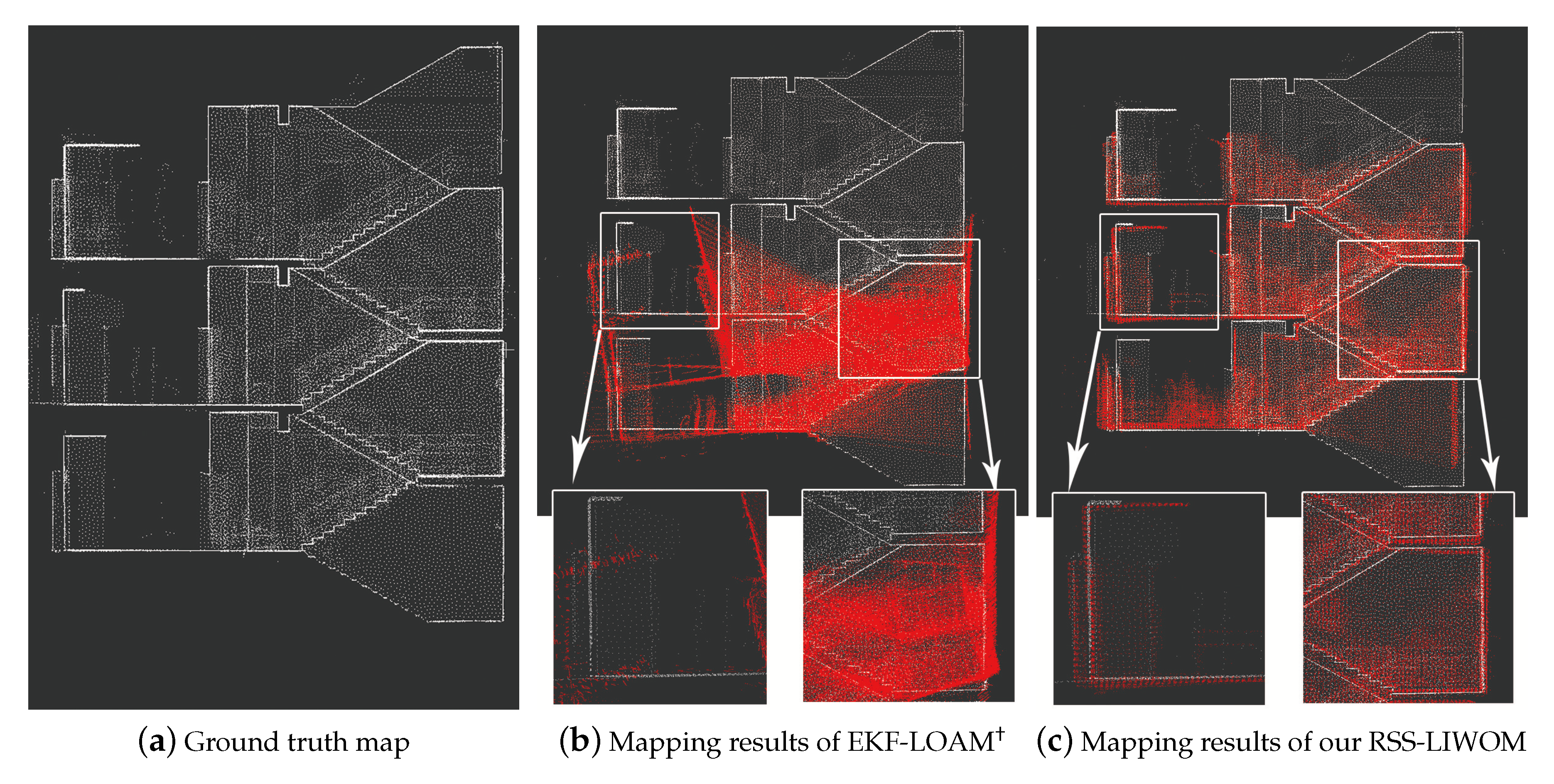
5.2. Evaluation on Mapping Quality

In this section, we evaluate the mapping quality of our RSS-LIWOM compared to the baselines with respect to the ground truth map obtained by the Faro FocusS350 scanner. The real scene and corresponding ground truth map are shown in Figure 7. The experimental scenes include a narrow corridor, open space and stairway such that the complexity and comprehensiveness of the scene are quite challenging in the ground-based unmanned platform SLAM problem. To further demonstrate our experimental scene, we provide links (https://github.com/nubot-nudt/RSS_LOAM_Datasets, accessed on 6 July 2023) to download the experimental datasets and the ground truth measurement-based FocusS350 scanner. We employ two metrics to quantitatively evaluate the accuracy of the reconstructed maps of each methods. The first metric measures the accuracy of the reconstructed map using the Chamfer distance, which computes the average distance between each point in the reconstructed map to its nearest counterpart in the ground truth map. The second metric is the mapping coverage rate, which represents the percentage of map points that are accurately reconstructed. We define accurately reconstructed map points as those whose distance to the nearest point in the ground truth map is below a threshold of 0.2 m. To ensure a fair comparison, the mapping results of all the methods are voxelized using a consistent voxel size of 0.1 m. Additionally, we provide the number of points in the mapping result for each method.

The quantitative mapping results for both scenes are presented in

Table 4. Comparison of mapping quality.

Scene	Method	Chamfer Distance	Cover Rate (%)	Number of Points
Campus	FAST-LIO2	1.44	16.2	$4.3\times {10}^5$
	EKF-LOAM${}^{†}$	0.69	62.7	$2.7\times {10}^5$
	RSS-LIWOM (Ours)	0.67	70.2	$4.8\times {10}^5$
Stairway	FAST-LIO2	-	-	-
	EKF-LOAM${}^{†}$	1.50	36.2	$3.1\times {10}^4$
	RSS-LIWOM (Ours)	0.37	70.0	$4.4\times {10}^4$

The threshold for cover rate is 0.2 m. Faro FocusS350 scanner points number is $5.5\times {10}^4$ in the stairway scene and is $4.3\times {10}^5$ in the campus scene. EKF-LOAM${}^{†}$ represents EKF-LOAM with mechanical LiDAR. Bold numbers indicate the best results.

. As can be seen, our RSS-LIWOM, utilizing a rotating solid-state LiDAR, benefits from a larger FOV and accurate odometry estimation, resulting in the highest mapping accuracy and coverage rate in both the campus and stairway scenes. Specifically, in the campus scene, our approach achieves the lowest Chamfer distance of 0.67 m and the highest coverage rate of 70.2%. In the stairway scene, our approach consistently achieves the lowest Chamfer distance of 0.37 m and a coverage rate of 70%. In contrast, FAST-LIO2 is limited by its narrow FOV solid-state LiDAR, which leads to inaccurate odometry estimation. Consequently, FAST-LIO2 exhibits suboptimal mapping accuracy in the campus scene and fails to produce meaningful results in the stairway scene. The performance of EKF-LOAM varies significantly between the two scenes. It achieves comparable mapping accuracy to our approach in the campus scene but does not perform well in the stairway scene. EKF-LOAM also suffers from the issue of feature degeneration in narrow scenes, which contributes to its poor performance. Overall, the larger FOV and accurate odometry estimation provided by our rotating solid-state LiDAR enable our approach to outperform FAST-LIO2 and EKF-LOAM in terms of mapping accuracy and coverage rate in both scenes.

To better demonstrate the advantages of our RSS-LIWOM in mapping, we provide more qualitative visualization results of different methods compared with the ground truth maps. We first visualize the mapping result in the campus scene in Figure 8. The red dots represent the mapping results of our RSS-LIWOM and baseline methods, while the white dots represent the ground truth map points. As can be seen, our reconstructed maps align better than other methods with the ground truth maps, which reveals that, benefiting from high-quality point cloud and accurate odometry estimation, RSS-LIWOM performs better and captures more environmental details than the baseline methods. FAST-LIO2 performs sub-optimally with significant deviation from the ground truth map due to feature degradation. Although EKF-LOAM has similar overall mapping performance as RSS-LIWOM, it cannot capture as many details as RSS-LIWOM. We zoom in on two typical areas in the campus scene, a narrow corridor and the starting/ending points; our RSS-LIWOM overlaps better with the ground truth map than the baselines and achieves a higher coverage rate.

We also visualize the mapping results in the stairway scene. As shown in Figure 9c, our RSS-LIWOM performs well in the climbing stairway scene, achieving a high degree of overlap with the ground truth map and clear distinction between different floors. In contrast, the mapping accuracy of EKF-LOAM significantly decreases when climbing stairs (as shown in Figure 9b). This is mainly due to the inaccurate vertical odometry estimation of EKF-LOAM.

We furthermore provide a qualitative comparison of different methods in terms of heat maps, shown in Figure 10. In the figure, different colors represent the magnitude of the Chamfer distance for each point, with cyan indicating smaller distances and orange indicating larger ones. The visualization results provide a more intuitive demonstration of the advantages of our algorithm in terms of the Chamfer distance in the corridor and hall of the campus, compared with FAST-LIO2 and EKF-LOAM.

5.3. Smoothness of Velocity Estimation

To further demonstrate the improvement of our method through the fusion wheel encoder measurements, we compare RSS-LIWOM with RSS-LIWOM${}^{\times }$ in terms of the smoothness of the velocity estimation.

We evaluate the velocity estimation based on the hypothesis that the robot’s movements should be continual and smooth, rather than high-frequency oscillations. As shown in Figure 11, our RSS-LIWOM achieves smoother velocity estimation by incorporating wheel encoder measurements, outperforming methods that do not utilize such information.

6. Discussion

In this work, we designed a rotating solid-state LiDAR sensory platform and develop a LIWOM framework named RSS-LIWOM that fuses LiDAR, IMU, and wheel encoder data for odometry and mapping on ground unmanned platforms, such as track robots. The rotating solid-state LiDAR has a larger scanning range and stronger ability to capture detailed information in the environment, compared to original solid-state LiDAR and mechanism LiDAR. The LIWOM framework uses wheel encoder measurements as an observation for velocity, which is not present in existing LIOM frameworks. By combining the rotating solid-state LiDAR and LIWOM framework, our RSS-LIWOM achieves a robust and accurate LIWOM system.

We conducted extensive experiments to thoroughly evaluate our approach using our own-designed track robot, which navigated through both indoor-outdoor mixed campus and stairway environments. In the campus environment, the robot followed a predetermined trajectory and returned to the starting point. We compared our approach with the baseline in terms of the odometry estimation and mapping results, and our approach outperformed the baselines by exhibiting the lowest odometry drift. In the stair scene experiment, we manipulated the robot to climb stairs across multiple floors. Our approach demonstrated minimal odometry drift in estimating the vertical orientation. Additionally, we generated a highly precise 3D map using the Faro FocusS350 scanner as the ground truth for evaluating the mapping quality. When comparing the Chamfer distance with the ground truth, our RSS-LIWOM achieved the best results. These experiments validate the localization and mapping capabilities of our approach on ground unmanned platforms within building scenes.

In future work, we aim to improve our approach by enhancing map management with a confidence factor for greater robustness and adaptability. We also plan to integrate trajectory planning and object recognition, enabling robots to navigate complex environments more efficiently. These advancements will make our approach more valuable for applications such as search and rescue, exploration, and transportation.

References

1. Yan, L.; Dai, J.; Zhao, Y.; Chen, C. Real-Time 3D Mapping in Complex Environments Using a Spinning Actuated LiDAR System. Remote Sens. 2023, 15, 963. [Google Scholar] [CrossRef]
2. Chen, W.; Shang, G.; Ji, A.; Zhou, C.; Wang, X.; Xu, C.; Li, Z.; Hu, K. An overview on visual slam: From tradition to semantic. Remote Sens. 2022, 14, 3010. [Google Scholar] [CrossRef]
3. Mur-Artal, R.; Montiel, J.M.M.; Tardos, J.D. ORB-SLAM: A versatile and accurate monocular SLAM system. IEEE Trans. Robot. (TRO) 2015, 31, 1147–1163. [Google Scholar] [CrossRef] [Green Version]
4. Wang, R.; Wan, W.; Wang, Y.; Di, K. A new RGB-D SLAM method with moving object detection for dynamic indoor scenes. Remote Sens. 2019, 11, 1143. [Google Scholar] [CrossRef] [Green Version]
5. Zhang, M.; Chen, Y.; Li, M. Vision-Aided Localization For Ground Robots. In Proceedings of the 2019 IEEE/RSJ International Conference on Intelligent Robots and Systems (IROS), Macau, China, 3–8 November 2019. [Google Scholar]
6. Liu, J.; Gao, W.; Hu, Z. Visual-Inertial Odometry Tightly Coupled with Wheel Encoder Adopting Robust Initialization and Online Extrinsic Calibration. In Proceedings of the 2019 IEEE/RSJ International Conference on Intelligent Robots and Systems (IROS), Macau, China, 3–8 November 2019. [Google Scholar]
7. Xia, X.; Meng, Z.; Han, X.; Li, H.; Tsukiji, T.; Xu, R.; Zheng, Z.; Ma, J. An automated driving systems data acquisition and analytics platform. Transp. Res. Part C Emerg. Technol. 2023, 151, 104120. [Google Scholar] [CrossRef]
8. Liu, W.; Xia, X.; Xiong, L.; Lu, Y.; Gao, L.; Yu, Z. Automated vehicle sideslip angle estimation considering signal measurement characteristic. IEEE Sens. J. 2021, 21, 21675–21687. [Google Scholar] [CrossRef]
9. Wang, D.; Watkins, C.; Xie, H. MEMS mirrors for LiDAR: A review. Micromachines 2020, 11, 456. [Google Scholar] [CrossRef] [PubMed]
10. Liu, Z.; Zhang, F.; Hong, X. Low-Cost Retina-Like Robotic Lidars Based on Incommensurable Scanning. IEEE/ASME Trans. Mechatron. 2022, 27, 58–68. [Google Scholar] [CrossRef]
11. Chen, Y.; Medioni, G. Object modeling by registration of multiple range images. In Proceedings of the 1991 IEEE International Conference on Robotics and Automation (ICRA), Sacramento, CA, USA, 9–11 April 1991. [Google Scholar]
12. Zhang, Z. Iterative point matching for registration of free-form curves and surfaces. Int. J. Comput. Vis. (IJCV) 1994, 13, 119–152. [Google Scholar] [CrossRef]
13. Segal, A.; Haehnel, D.; Thrun, S. Generalized-icp. In Proceedings of the Robotics: Science and Systems, Seattle, WA, USA, 28 June–1 July 2009. [Google Scholar]
14. Besl, P.; McKay, N.D. A method for registration of 3-D shapes. IEEE Trans. Pattern Anal. Mach. Intell. 1992, 14, 239–256. [Google Scholar] [CrossRef] [Green Version]
15. Vizzo, I.; Guadagnino, T.; Mersch, B.; Wiesmann, L.; Behley, J.; Stachniss, C. KISS-ICP: In Defense of Point-to-Point ICP Simple, Accurate, and Robust Registration If Done the Right Way. IEEE Robot. Autom. Lett. (RA-L) 2023, 8, 1029–1036. [Google Scholar] [CrossRef]
16. Zhang, J.; Singh, S. LOAM: Lidar odometry and mapping in real-time. In Proceedings of the Robotics: Science and Systems, Berkeley, CA, USA, 12–16 July 2014. [Google Scholar]
17. Shan, T.; Englot, B. LeGO-LOAM: Lightweight and Ground-Optimized Lidar Odometry and Mapping on Variable Terrain. In Proceedings of the 2018 IEEE/RSJ International Conference on Intelligent Robots and Systems (IROS), Madrid, Spain, 1–5 October 2018. [Google Scholar]
18. Lin, J.; Zhang, F. Loam livox: A fast, robust, high-precision LiDAR odometry and mapping package for LiDARs of small FoV. In Proceedings of the 2020 IEEE International Conference on Robotics and Automation (ICRA), Paris, France, 31 May–31 August 2020. [Google Scholar]
19. Chen, X.; Milioto, A.; Palazzolo, E.; Giguère, P.; Behley, J.; Stachniss, C. SuMa++: Efficient LiDAR-based Semantic SLAM. In Proceedings of the 2019 IEEE/RSJ International Conference on Intelligent Robots and Systems (IROS), Macau, China, 3–8 November 2019. [Google Scholar]
20. Chen, X.; Läbe, T.; Milioto, A.; Röhling, T.; Behley, J.; Stachniss, C. OverlapNet: A Siamese Network for Computing LiDAR Scan Similarity with Applications to Loop Closing and Localization. Auton. Robot. 2021, 46, 61–81. [Google Scholar] [CrossRef]
21. Shi, C.; Chen, X.; Huang, K.; Xiao, J.; Lu, H.; Stachniss, C. Keypoint matching for point cloud registration using multiplex dynamic graph attention networks. IEEE Robot. Autom. Lett. 2021, 6, 8221–8228. [Google Scholar] [CrossRef]
22. Guadagnino, T.; Chen, X.; Sodano, M.; Behley, J.; Grisetti, G.; Stachniss, C. Fast Sparse LiDAR Odometry Using Self-Supervised Feature Selection on Intensity Images. IEEE Robot. Autom. Lett. 2022, 7, 7597–7604. [Google Scholar] [CrossRef]
23. Shi, C.; Chen, X.; Lu, H.; Deng, W.; Xiao, J.; Dai, B. RDMNet: Reliable Dense Matching Based Point Cloud Registration for Autonomous Driving. arXiv 2023, arXiv:2303.18084. [Google Scholar]
24. Deng, J.; Chen, X.; Xia, S.; Sun, Z.; Liu, G.; Yu, W.; Pei, L. NeRF-LOAM: Neural Implicit Representation for Large-Scale Incremental LiDAR Odometry and Mapping. arXiv 2023, arXiv:2303.10709. [Google Scholar]
25. Shan, T.; Englot, B.; Meyers, D.; Wang, W.; Ratti, C.; Rus, D. LIO-SAM: Tightly-coupled Lidar Inertial Odometry via Smoothing and Mapping. In Proceedings of the 2020 IEEE/RSJ International Conference on Intelligent Robots and Systems (IROS), Las Vegas, NV, USA, 24 October–24 January 2020. [Google Scholar]
26. Cattaneo, D.; Vaghi, M.; Valada, A. LCDNet: Deep Loop Closure Detection and Point Cloud Registration for LiDAR SLAM. IEEE Trans. Robot. 2022, 38, 2074–2093. [Google Scholar] [CrossRef]
27. Barros, T.; Garrote, L.; Pereira, R.; Premebida, C.; Nunes, U.J. AttDLNet: Attention-based DL Network for 3D LiDAR Place Recognition. arXiv 2021, arXiv:2106.09637. [Google Scholar]
28. Xia, Y.; Xu, Y.; Li, S.; Wang, R.; Du, J.; Cremers, D.; Stilla, U. SOE-Net: A Self-Attention and Orientation Encoding Network for Point Cloud based Place Recognition. In Proceedings of the 2021 IEEE/CVF Conference on Computer Vision and Pattern Recognition (CVPR), Nashville, TN, USA, 20–25 June 2021. [Google Scholar]
29. Chen, X.; Li, S.; Mersch, B.; Wiesmann, L.; Gall, J.; Behley, J.; Stachniss, C. Moving Object Segmentation in 3D LiDAR Data: A Learning-based Approach Exploiting Sequential Data. IEEE Robot. Autom. Lett. (RA-L) 2021, 6, 6529–6536. [Google Scholar] [CrossRef]
30. Chen, X.; Mersch, B.; Nunes, L.; Marcuzzi, R.; Vizzo, I.; Behley, J.; Stachniss, C. Automatic Labeling to Generate Training Data for Online LiDAR-Based Moving Object Segmentation. IEEE Robot. Autom. Lett. (RA-L) 2022, 7, 6107–6114. [Google Scholar] [CrossRef]
31. Mersch, B.; Chen, X.; Vizzo, I.; Nunes, L.; Behley, J.; Stachniss, C. Receding Moving Object Segmentation in 3D LiDAR Data Using Sparse 4D Convolutions. IEEE Robot. Autom. Lett. (RA-L) 2022, 7, 7503–7510. [Google Scholar] [CrossRef]
32. Liu, W.; Quijano, K.; Crawford, M.M. YOLOv5-Tassel: Detecting Tassels in RGB UAV Imagery with Improved YOLOv5 Based on Transfer Learning. IEEE J. Sel. Top. Appl. Earth Obs. Remote Sens. 2022, 15, 8085–8094. [Google Scholar] [CrossRef]
33. Meng, Z.; Xia, X.; Xu, R.; Liu, W.; Ma, J. HYDRO-3D: Hybrid Object Detection and Tracking for Cooperative Perception Using 3D LiDAR. IEEE Trans. Intell. Veh. 2023, 1–13. [Google Scholar] [CrossRef]
34. Chen, H.; Wu, W.; Zhang, S.; Wu, C.; Zhong, R. A GNSS/LiDAR/IMU Pose Estimation System Based on Collaborative Fusion of Factor Map and Filtering. Remote Sens. 2023, 15, 790. [Google Scholar] [CrossRef]
35. Chen, X.; Zhang, H.; Lu, H.; Xiao, J.; Qiu, Q.; Li, Y. Robust SLAM system based on monocular vision and LiDAR for robotic urban search and rescue. In Proceedings of the 2017 IEEE International Symposium on Safety, Security and Rescue Robotics (SSRR), Shanghai, China, 11–13 October 2017; pp. 41–47. [Google Scholar]
36. Yang, X.; Lin, X.; Yao, W.; Ma, H.; Zheng, J.; Ma, B. A Robust LiDAR SLAM Method for Underground Coal Mine Robot with Degenerated Scene Compensation. Remote Sens. 2022, 15, 186. [Google Scholar] [CrossRef]
37. Zhen, W.; Zeng, S.; Soberer, S. Robust localization and localizability estimation with a rotating laser scanner. In Proceedings of the 2017 IEEE International Conference on Robotics and Automation (ICRA), Singapore, 29 May–3 June 2017. [Google Scholar]
38. Geneva, P.; Eckenhoff, K.; Yang, Y.; Huang, G. Lips: Lidar-inertial 3d plane slam. In Proceedings of the 2018 IEEE/RSJ International Conference on Intelligent Robots and Systems (IROS), Madrid, Spain, 1–5 October 2018. [Google Scholar]
39. Bry, A.; Bachrach, A.; Roy, N. State estimation for aggressive flight in GPS-denied environments using onboard sensing. In Proceedings of the 2012 IEEE International Conference on Robotics and Automation (ICRA), Saint Paul, MN, USA, 14–18 May 2012. [Google Scholar]
40. Xu, C.; Zhang, H.; Gu, J. Scan Context 3D Lidar Inertial Odometry via Iterated ESKF and Incremental K-Dimensional Tree. In Proceedings of the 2022 IEEE Canadian Conference on Electrical and Computer Engineering (CCECE), Halifax, NS, Canada, 18–20 September 2022. [Google Scholar]
41. Sola, J. Quaternion kinematics for the error-state Kalman filter. arXiv 2017, arXiv:1711.02508. [Google Scholar]
42. Xiong, L.; Xia, X.; Lu, Y.; Liu, W.; Yu, Z. IMU-based Automated Vehicle Body Sideslip Angle and Attitude Estimation Aided by GNSS using Parallel Adaptive Kalman Filters. IEEE Trans. Veh. Technol. 2020, 69, 10668–10680. [Google Scholar] [CrossRef]
43. Xia, X.; Xiong, L.; Lu, Y.; Gao, L.; Yu, Z. Vehicle sideslip angle estimation by fusing inertial measurement unit and global navigation satellite system with heading alignment. Mech. Syst. Signal Process. 2021, 150, 107290. [Google Scholar] [CrossRef]
44. Xia, X.; Hashemi, E.; Xiong, L.; Khajepour, A. Autonomous vehicle kinematics and dynamics synthesis for sideslip angle estimation based on consensus kalman filter. IEEE Trans. Control Syst. Technol. 2022, 31, 179–192. [Google Scholar] [CrossRef]
45. Xu, W.; Zhang, F. FAST-LIO: A Fast, Robust LiDAR-Inertial Odometry Package by Tightly-Coupled Iterated Kalman Filter. IEEE Robot. Autom. Lett. (RA-L) 2021, 6, 3317–3324. [Google Scholar] [CrossRef]
46. Xu, W.; Cai, Y.; He, D.; Lin, J.; Zhang, F. FAST-LIO2: Fast Direct LiDAR-Inertial Odometry. IEEE Trans. Robot. (TRO) 2022, 38, 2053–2073. [Google Scholar] [CrossRef]
47. Bai, C.; Xiao, T.; Chen, Y.; Wang, H.; Zhang, F.; Gao, X. Faster-LIO: Lightweight Tightly Coupled Lidar-Inertial Odometry Using Parallel Sparse Incremental Voxels. IEEE Robot. Autom. Lett. (RA-L) 2022, 7, 4861–4868. [Google Scholar] [CrossRef]
48. Nießner, M.; Zollhöfer, M.; Izadi, S.; Stamminger, M. Real-time 3D reconstruction at scale using voxel hashing. ACM Trans. Graph. 2013, 32, 1–11. [Google Scholar] [CrossRef] [Green Version]
49. Júnior, G.P.C.; Rezende, A.M.C.; Miranda, V.R.F.; Fernandes, R.; Azpúrua, H.; Neto, A.A.; Pessin, G.; Freitas, G.M. EKF-LOAM: An Adaptive Fusion of LiDAR SLAM with Wheel Odometry and Inertial Data for Confined Spaces with Few Geometric Features. IEEE Trans. Autom. Sci. Eng. (T-ASE) 2022, 19, 1458–1471. [Google Scholar] [CrossRef]
50. Yuan, Z.; Lang, F.; Xu, T.; Yang, X. LIW-OAM: Lidar-Inertial-Wheel Odometry and Mapping. arXiv 2023, arXiv:2302.14298. [Google Scholar]
51. Zhu, F.; Ren, Y.; Zhang, F. Robust real-time lidar-inertial initialization. In Proceedings of the 2022 IEEE/RSJ International Conference on Intelligent Robots and Systems (IROS), Kyoto, Japan, 23–27 October 2022. [Google Scholar]
52. Teschner, M. Optimized Spatial Hashing for Collision Detection of Deformable Objects. Vis. Model. Vis. 2003, 3, 47–54. [Google Scholar]
Figure 1. (a) Rotating solid-state LiDAR, (b) experimental robot, (c) mapping result of campus.
Remotesensing 15 04040 g001
Figure 2. The scanning result of original solid-state LiDAR and our rotating solid-state LiDAR. (a) One scanning of original solid-state LiDAR. (b) The result of two seconds of scanning in the same place of original solid-state LiDAR. (c) The result of two seconds of scanning obtained by our rotating solid-state LiDAR.
Remotesensing 15 04040 g002
Figure 3. Assembly error between the LiDAR and motor.
Remotesensing 15 04040 g003
Figure 4. Diagram of calibration showing the relationship of different measurements.
Remotesensing 15 04040 g004
Figure 5. System overview of our approach. The system can be separated into two parts: state estimation and mapping. In state estimation, an iterated Kalman filter is adopted to estimate state variables. IMU measurements are used for integration to generate state prediction. It then updates the velocity state by fusing the wheel encoder, transforms raw points from the LiDAR frame to the IMU frame and compensates for motion distortion. LiDAR scanning after motion compensation is used to compute the residual to optimize the pose to obtain the final odometry result. In the mapping module, the new scan is then added to the map that consists of a hash structure and the updated mapping result.
Remotesensing 15 04040 g005
Figure 6. LiDAR measurements model. Red point is the point in scan, blue points are the points in the map near the red point, and the vector from the plane to the red point is the normal and residual.
Remotesensing 15 04040 g006
Figure 7. Real scene and ground truth map of our experimental environments. (a) Real scene photos of our experimental environments. (b) The ground truth map of our experimental environments.
Remotesensing 15 04040 g007
Figure 8. The mapping results of (a) FAST-LIO2, (b) EKF-LOAM , and (c) our RSS-LIWOM. The white point cloud is the ground truth map points measured by Faro FocusS350 scanner and the red point cloud is the estimated result.
Remotesensing 15 04040 g008aRemotesensing 15 04040 g008b
Figure 9. (a) The ground truth map and the mapping result of (b) EKF-LOAM  and (c) our RSS-LIWOM. Different approach in stair scene. White point cloud is ground truth map measured by Faro FocusS350 scanner, and the red point cloud is the estimated result.
Remotesensing 15 04040 g009
Figure 10. The visual results of Chamfer distance and cover rate in typical part of campus scene. (a) FAST-LIO2 in corridor, (b) EKF-LOAM in corridor, (c) RSS-LIWOM in corridor, (d) FAST-LIO2 in hall, (e) EKF-LOAM in hall and (f) RSS-LIWOM in hall.
Remotesensing 15 04040 g010
Figure 11. The velocity estimation of RSS-LIWOM (blue line) and RSS-LIWOM ×  (red line). (a) The velocity estimation in campus. (b) The velocity estimation in stairway.
Remotesensing 15 04040 g011