Article

Quantitative Precipitation Estimation in the Tianshan Mountains Based on Machine Learning

1
Institute of Desert Meteorology, China Meteorological Administration, Urumqi 830002, China
2
State Key Laboratory of Cryospheric Science, Northwest Institute of Eco-Environment and Resources, Chinese Academy of Sciences, Lanzhou 730000, China
3
National Field Science Observation and Research Station of Yulong Snow Mountain Cryosphere and Sustainable Development, Northwest Institute of Eco-Environment and Resources, Chinese Academy of Sciences, Lanzhou 730000, China
*
Author to whom correspondence should be addressed.
Remote Sens. 2023, 15(16), 3962; https://doi.org/10.3390/rs15163962
Submission received: 9 June 2023 / Revised: 1 August 2023 / Accepted: 8 August 2023 / Published: 10 August 2023

Abstract

:
Precipitation in the Tianshan Mountains is abundant, and the quantitative estimation of precipitation in mountainous areas is important to the application and evaluation of regional water resources. With remote sensing technology, satellite inversion of precipitation can estimate precipitation in mountainous areas. However, the Tianshan Mountain terrain is complex, and the spatiotemporal variation in precipitation is large, so the accuracy of satellite precipitation inversion is not high. Here, precipitation data from around 1000 automatic weather stations in the Tianshan Mountains are used to study the correction technology of the Integrated Multisatellite Retrievals for the Global Precipitation Measurement (GPM) mission’s (IMERG) monthly precipitation products using stepwise regression (STEP), geographically weighted regression (GWR), and random forest (RF). First, geographic information system technology was used to extract topographic variables from a digital elevation model, and vegetation indexes, which are important precipitation indicators, were introduced as explanatory factors to correct satellite precipitation data. Second, GPM IMERG precipitation was corrected by establishing the stepwise regression, the geographically weighted regression model, and the random forest model. The three correction methods can improve the GPM IMERG in terms of relative bias, root mean square error, correlation coefficient, and Nash–Sutcliffe efficiency, while the random forest method shows better corrections than the two traditional methods. For dense rainfall stations, the geographically weighted regression method is as effective as random forest. For different altitudes, the results show that RF has the best correction effect in the first three zones, but the correction effect in the last zone (over 3000 m) is worse than STEP. This study provides a practical reference method for estimating precipitation data in the non-rainfall observation area, which helps to deepen the scientific understanding of the water resource distribution in the Tianshan Mountains and provide scientific data support for regional hydrological and meteorological research.

1. Introduction

Precipitation is an important part of the water cycle on Earth and has an important impact on ecosystems, agriculture, and water resource management [1,2]. At present, there are three main ways to obtain precipitation observation information: rain gauges, ground-based radar, and satellite remote sensing. Station observations are highly accurate; however, stations cannot effectively reflect the spatial variation characteristics of precipitation in mountainous areas. Therefore, spatial representations are insufficient. The precipitation data derived from meteorological radar echoes are advantageous due to regional estimations. However, the Z-I (reflectivity–rainfall intensity) relationship varies greatly in different precipitation systems, seasons, and regions, which affects the precipitation accuracy of radar estimation. In addition, radar detection is easily limited by ground object blocking, beam effect, and velocity ambiguity, so it is difficult to apply over a wide range of mountainous areas. The rapid development of remote sensing and geographic information science provides a new method for the simultaneous observation of large-scale precipitation. Satellite-retrieved precipitation has the unique advantages of all-weather, global coverage, and accurately reflecting the “spatial distribution” of precipitation, which makes it an important means to systematically understand the regional and global precipitation distribution and its changes. However, the spatial resolution of satellite precipitation products is low, and it cannot meet the needs of hydrological and meteorological research at the basin scale. In addition, the terrain of the Tianshan Mountains is complex, and the spatial distribution of precipitation is obviously different. Therefore, the satellite precipitation inversion algorithm has great uncertainty in this region; thus, the accuracy of satellite precipitation products is relatively low [3,4]. It is necessary to study the correction of satellite precipitation products before application [5].
As an important part of high Asia, the Tianshan Mountains are the largest mountain system in central Asia, known as the “Central Asian Water Tower”, and 65% of the rivers in Xinjiang originate from this region [6]. The Tianshan Mountains are not only a watershed in the climate of northern and southern Xinjiang but are also an important natural barrier that affects the weather, climate, and ecological environment of Xinjiang and even the central and western regions of China. Precipitation in mountainous areas is the most important part of the hydrological cycle in arid areas and an important source of water resources [7]. How to obtain high-resolution regional precipitation distribution in this area is an urgent problem that needs to be solved.

2. Materials and Methods

2.1. Study Area

In central Asia, the broadest part of the Tianshan Mountains stretches across Xinjiang, with a length of 1700 km from east to west and a width of approximately 250 to 350 km from north to south. It is the geographical dividing line between northern and southern Xinjiang, and its terrain units, which include mountains, basins, valleys, and piedmont plains, constitute a unique landform. The region belongs to the alpine mountain area, with an average altitude of approximately 4000 m. Due to the influence of westerly circulation and topography, the distribution of precipitation in the region is extremely uneven, with large precipitation in summer and little precipitation in winter. The precipitation gradually decreases from west to east, and the precipitation on the northern slope is significantly greater than that on the southern slope. On the northern slope of the Tianshan Mountains, the average annual precipitation can reach 500 to 700 mm. In addition to its unique terrain and precipitation conditions, the Tianshan Mountains in the northwest arid region form a unique “wet island” landscape.

2.2. Data

2.2.1. Satellite Data Sets

  • GPM IMERG
GPM is the subsequent precipitation plan of the Tropical Rainfall Measuring Mission (TRMM), which can provide global rainfall and snowfall data, including data within 3 h based on microwaves and half an hour based on microwave infrared. Compared with TRMM, GPM has a higher precipitation observation ability. Its dual-frequency radar can detect very weak signals. At the same time, its microwave radiometer can also observe trace rainfall and solid precipitation more accurately. Therefore, GPM is of great significance for studying precipitation in middle and high latitudes, such as the Tianshan Mountains in Xinjiang [8,9]. The IMERG data in this study are derived from GPM’s Day-1 multisatellite precipitation estimation algorithm [8]. IMEG products have three modes (early, late, and final runs), and users can choose the right product according to their research needs. The three-stage IMEG final run product was provided by the GPM in March 2014. A rain gauge from the Global Precipitation Climatology Centre (GPCC) was introduced into the final run product to correct the data, so the product provides more accurate results and is considered a research-level product [8]. The above three products provide a 0.5 h, 0.1° × 0.1° resolution, 60°N–60°S spatial coverage data set (3IMERGHH), and finally, a 0.1° × 0.1° monthly precipitation data set is generated and combined with the rain gauge data (3IMERGM) [8,9]. The latest version of the IMERG final run is V06.
2.
NDVI
The NDVI is an indicator of vegetation activity and biomass [10,11,12]. The NDVI data used in this study were obtained by the Moderate Resolution Imaging Spectroradiometer (MODIS) on the EOS/Terra satellite (https://wist.echo.nasa.gov (accessed on 1 August 2022)). The land three-level standard data product MOD13A3 was selected, and the content is a rasterized three-level since curve projection grid product with a monthly resolution of 1 km. During processing of the product, the algorithm absorbs all 1 km products covering the whole month in 16 days. If there are no clouds in the atmosphere, the time-weighted average method is used, or the minimum value is used to prevent cloud influence. These data can be used as inputs to simulate global biogeochemical and hydrological processes and global and regional climates, as well as to characterize biological properties and processes on the Earth’s surface, including primary production and land cover change.
3.
DEM
This study used the DEM data provided by ASTER GDEM with a resolution of 1 arc s, which was derived from the detailed observations of NASA’s Terra satellite. It covers 99% of the Earth’s land surface and covers all land areas between 83°N and 83°S. By using the functions of “Aspect”, “Slope”, “Hillshade”, “Curvature”, “Tabulate Area”, and “Zonal Statistics” in geographic information system software, this study successfully extracted a variety of topographic variables, including slope (SLP) [13], aspect (ASP) [14], curvature (CVT) [15], topographic wetness index (TWI) [16], and hillshade (HSHD) [14]. More detailed information is available in the literature [14,17].

2.2.2. Rain Gauge Data

The monthly precipitation data of the meteorological station were provided by the Information Center of the Xinjiang Meteorological Bureau. The precipitation data of 57 national stations (excluding 8 international exchange stations in the Tianshan Mountains) and more than 1000 regional automatic stations in the Tianshan Mountains were selected. The spatial distribution of rainfall stations is shown in Figure 1. The live site is divided into two parts, 90% for modeling and 10% as an independent data set to verify the accuracy of the corrected product. At present, the regional automatic stations in Xinjiang can only observe liquid precipitation and do not have the ability to observe solid precipitation. Therefore, this study selected the warm season period from May to September 2014–2017 to carry out research, and the live data passed strict quality control procedures.
According to the independence requirements of satellite precipitation data evaluation for stations, 194 GPCC stations in China have been used for bias correction of TRMM/GPM research-level products. In particular, there are 8 GPCC stations in the Tianshan Mountains of Xinjiang [3,18]. Therefore, we need to remove these 8 GPCC stations for objective and independent evaluation. Due to the sparse distribution of stations in Xinjiang, interpolation based on observation station data will produce serious errors. Therefore, this study used a more direct comparison to extract the stations that fall into the grid with a 0.1° × 0.1° resolution and match them with the grid. If two or more stations are in the same grid, their average precipitation is matched with the satellite estimates of the grid [19,20,21,22].

2.3. Methods

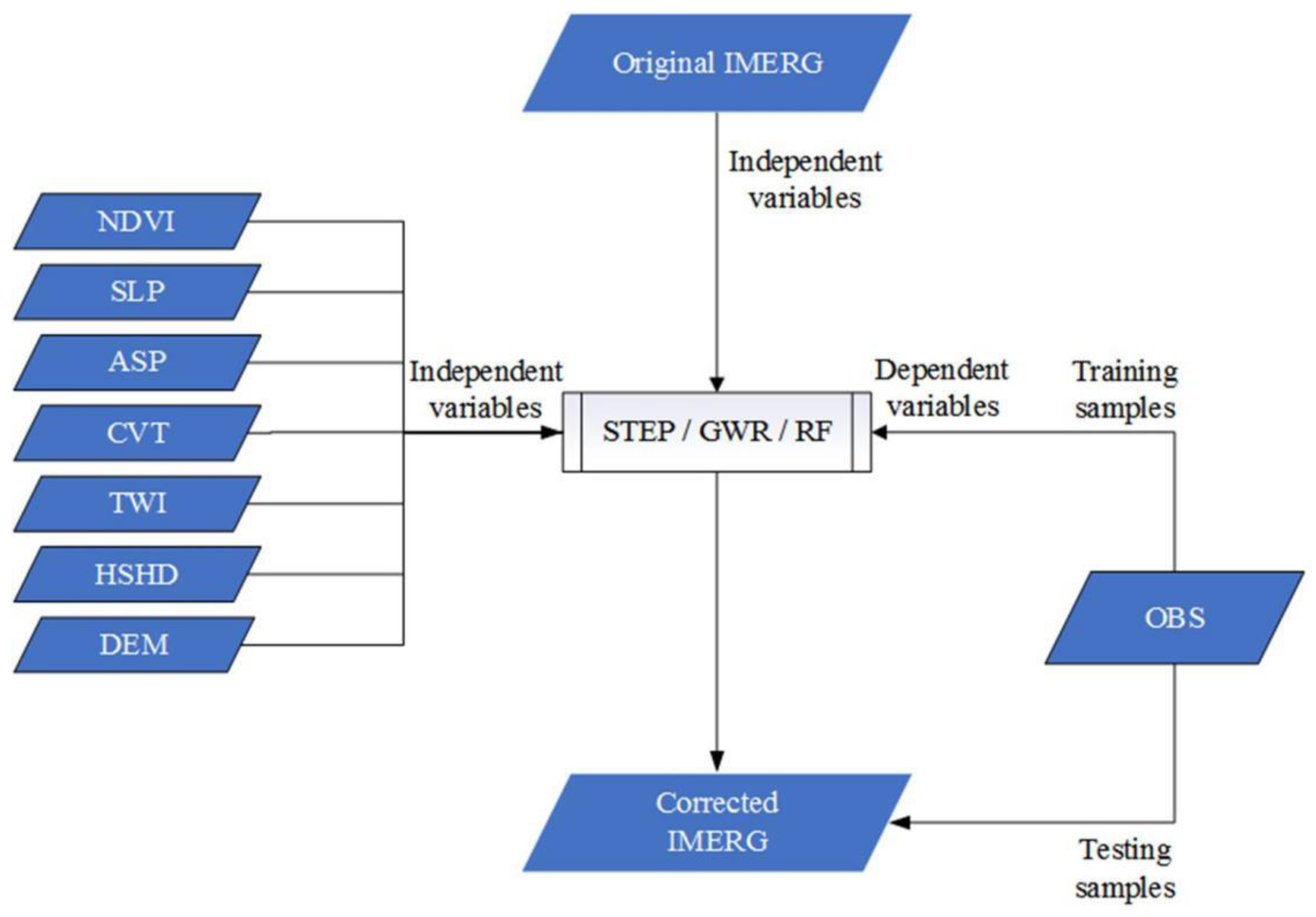
The distribution of precipitation in mountainous areas is very complex, which is not only related to the climate conditions but also influenced by terrain and altitude. Studying the impact of geographical and topographic factors on the distribution of precipitation has always been a hot topic in academia and application departments. In addition, vegetation represents a natural connection between soil, atmosphere, and water, and is an important indicator of ecology and environment. The Normalized Difference Vegetation Index (NDVI) is highly sensitive to the growth potential of surface vegetation and can reflect changes in surface vegetation cover to a certain extent. Therefore, NDVI is considered the best indicator of surface vegetation. Figure 2 shows the flow chart of the corrected methods in this study. By establishing the correction models with IMERG, NDVI, and various terrain factors (ASP, SLP, CVT, TWI, HSHD, and DEM) as independent variables and observed precipitation as a dependent variable, the original IMERG precipitation data over this region are corrected using STEP, GWR, and RF. The detailed description is as follows.

2.3.1. Stepwise Regression

The basic idea of stepwise regression is to introduce variables into the model one by one. The F test is carried out after each explanatory variable is introduced, and the t test is carried out one by one for the selected explanatory variables. When the original explanatory variables are no longer significant due to the introduction of the following explanatory variables, they are deleted to ensure that only significant variables are included in the regression equation before each new variable is introduced. This process is repeated until no significant explanatory variables are selected for the regression equation, and no nonsignificant explanatory variables are removed from the regression equation to ensure that the final set of explanatory variables is optimal [23,24]. In this study, the initial IMERG monthly precipitation, topographic factors, and the NDVI were used as independent variables, and the measured precipitation of the meteorological station was used as the dependent variable. The monthly regression equation from May to September was obtained using stepwise regression analysis. Then, we extracted the topographic variables, the NDVI and IMERG grid precipitation of each IMERG grid, and brought them into the monthly regression equation to obtain the IMERG grid precipitation (STEP) on a monthly scale corrected using the multiple regression equation. The regression modeling formula was obtained as follows:
P O B S = f P I M E R G , N D V I , T E R R + ε
In Equation (1), P O B S is the measured precipitation of the station, P I M E R G is the IMERG precipitation before correction, T E R R is the terrain factor variable value, and ε is the residual.

2.3.2. GWR

The GWR method was proposed by Brunsdon et al. in 1996 and has been widely used in spatial heterogeneity research [25,26,27]. The basic concept is the relationship between variables, which changes with the change in spatial location. By estimating the parameters of the relevant variables and explanatory variables at each given position in the study area, a regression model is established to obtain the best results. This study uses topographic variables, the NDVI and IMERG precipitation data, to establish a GWR regression model, as shown below.
Y j = β 0 u j , v j + i = 1 p β i u j , v j X i j + ε j
In Equation (2), Y j is the actual precipitation of the jth point, X i j is the IMERG precipitation, topographic variables, and NDVI values at point i around point j, β 0 u j , v j and β i u j , v j are the intercept and slope of point j, u j , v j is the coordinate of point j in two-dimensional space, and ε j is the residual. Different from the traditional global regression model, Equation (2) is based on the assumption that the closer the observation point is to point j, the greater the influence. The coefficient is the attenuation function of the observation distance around point j, which can be obtained by solving Equation (3).
β ^ u j , v j = X T W u j , v j X 1 X T W u j , v j Y
In Equation (3), β ^ u j , v j is the coefficient of point j, X and Y are independent variables and dependent variables, respectively, and W u j , v j is the weight matrix, which ensures that the closer to point j the position is, the greater the weight, and its value is obtained by the following formula.
ω i j = 1 d i j / b 2 2 d i j b ω i j = 0 d i j > b
In Equation (4), d i j is the distance between point j and the surrounding observation point i, and b is the bandwidth threshold.

2.3.3. Random Forest

RF consists of multiple decision trees. The modeling process first randomly selects 70% of the site data from the monthly data set as the training set and then randomly selects m features from the monthly M feature variables as the node index of a decision tree, where the minimum mean square error (MSE) is used as the branch standard for each node. The final prediction results are shown in Equation (5):
P ( x ) = 1 K n = 1 K t n ( x )
In Equation (5), P is the final precipitation prediction value, K is the number of the whole decision tree, n is the sample with put-back, and tn is each individual decision tree.
The test set of RF is also called out-of-bag samples. The importance ranking of each feature variable can be obtained by evaluating the results of out-of-bag samples. After removing some features with low importance, a new feature set is obtained. Multiple iterations are conducted according to this step, and the relatively poor features are gradually removed until the remaining feature number is m. Finally, the RF model is constructed by optimization based on all the iterated forests. According to this step, the formula is iterated many times, and the relatively poor features are gradually removed until the remaining feature number is m. Then, optimization is performed from all the iterated forests, and finally, RF model construction is completed.

2.3.4. Validation

The measured data from the stations are the most realistic precipitation monitoring data. In this study, 96 independent stations (accounting for 10% of all the stations) that did not participate in the correction processing were selected to test the effect of precipitation estimation products corrected by three correction methods (STEP, GWR, and RF) and compared with IMERG monthly precipitation data. Relative bias (RB), correlation coefficients (CC), root mean square error (RMSE), and Nash–Sutcliffe efficiency coefficients (NSE) were used to test the observed and predicted values. The equations are shown in Equations (6)–(9), where xi and yi represent estimated precipitation and observed precipitation, respectively. NSE is generally used to verify the hydrological model simulation results [28,29], and the value is negative infinity to 1. NSE is close to 1, indicating that the model has good quality and high reliability. NSE is close to 0, indicating that the simulation results are close to the average level of the observed values; that is, the overall results are credible, but the process simulation error is large. If NSE is far less than 0, the model is not credible.
RB = x i y i y i × 100 %
CC = x i x ¯ y i y ¯ x i x ¯ 2 y i y ¯ 2
RMSE = 1 n x i y i 2
NSE = 1 x i y i 2 x i x ¯ 2 × 100 %

3. Results

3.1. Importance Ranking of Predictive Factors

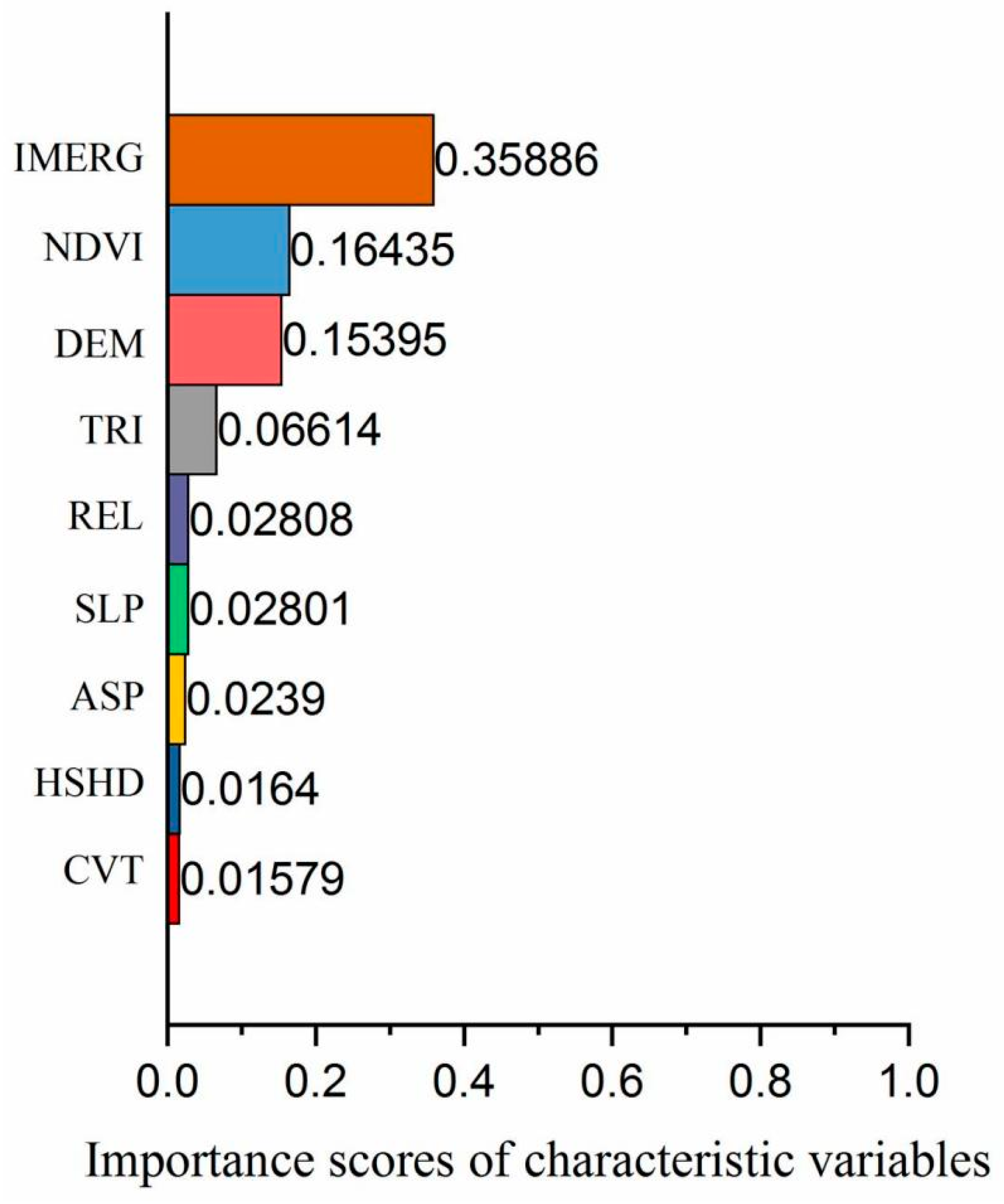
The RF provides an effective method to select relevant features from the dataset. The importance of the features is measured by the average impure attenuation of all the decision trees in the RF. Figure 3 shows the importance ranking of live precipitation and each characteristic variable in the whole data set. The figure shows that IMERG has the highest importance among all predictors, reaching 0.36, followed by the NDVI (0.16) and DEM (0.15), and the remainder are below 0.1. This is consistent with the contribution rate of explanatory factors in the stepwise regression study.

3.2. Overall Evaluation

In this study, the raw IMERG data (IMERG)-, stepwise regression (STEP)-, geographically weighted regression (GWR)-, and random forest (RF)-corrected grid precipitation were tested by using the measured monthly precipitation data of 959 independent stations in the Tianshan Mountains during the warm season (May–September) from 2014 to 2017. The accuracy of each site is evaluated by comparing the observed values and satellite-estimated precipitation, and the accuracy of the above three estimated data in the entire study area is comprehensively analyzed (Table 1). The results show that the correlation coefficients of IMERG, STEP, GWR, and RF with the observation data of meteorological stations are 0.56, 0.74, 0.79, and 0.81, respectively, which pass the confidence test level of 0.01. This finding shows that there is a significant linear correlation between these four predicted values and the observed data, and the correlation between precipitation data corrected by random forest and geographically weighted regression and actual data is higher. The Nash efficiency coefficients of the IMERG, STEP, GWR, and RF data are 0.31, 0.55, 0.62, and 0.66, respectively. According to its definition, the closer to 1 NSE is, the better the estimated value quality. Therefore, the estimation result of the random forest is the best. From the perspective of the root mean square error, the IMERG, STEP, GWR, and RF values are 27.41 cm, 22.63 cm, 20.94 cm, and 19.81 cm, respectively. The accuracy after correction is significantly improved compared with that before correction and is consistent with the correlation coefficient and NSE, and the random forest correction effect is the best.
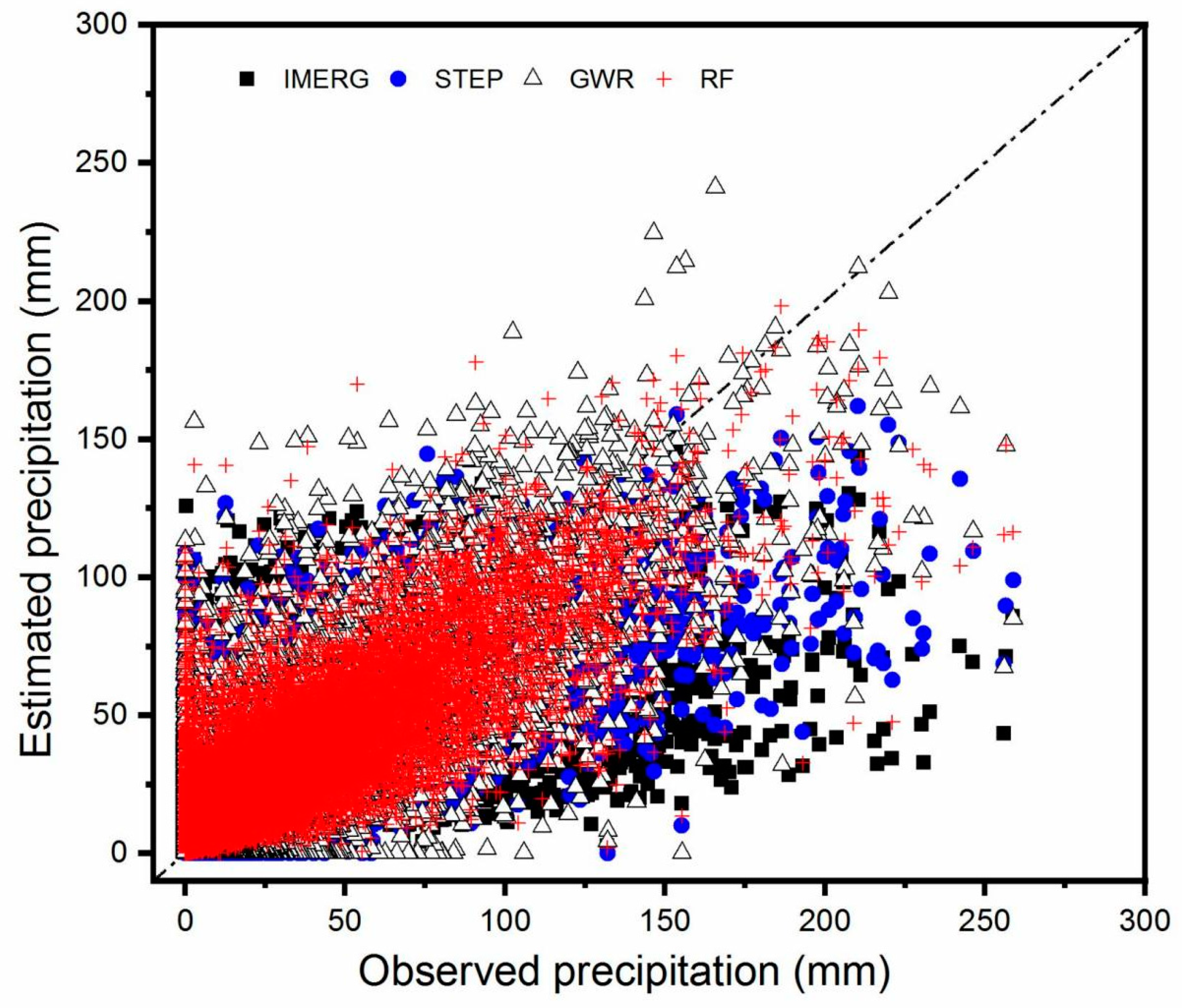
Figure 4 shows the scatter plots of the four estimation products and the actual precipitation. The figure shows that IMERG and STEP have the worst consistency with the actual precipitation and the most dispersed distribution. Especially in the 150–250 mm interval with large precipitation, there are many underestimation phenomena, while GWR and RF are significantly improved. Although GWR does not underestimate in the large value area, it is still relatively dispersed in the low value area. Overall, RF is most concentrated in both the high value area and the low value area, and it is evenly distributed around the 1:1 line.
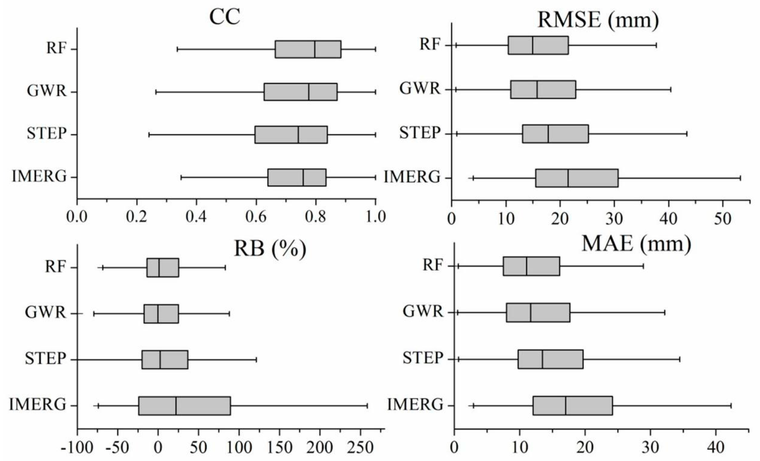
Figure 5 shows the boxplot distribution obtained from the CC, RMSE, RB, MAE, and other indicators of the 1067 sites. The boxplot is a method of describing data using five statistics from a set of data: minimum, the first quartiles, median, the third quartiles, and maximum. It can intuitively see whether the data are symmetrical, the degree of dispersion in the distribution, and other information. Figure 5 shows that the RF of the four estimation products is basically the most concentrated in each statistical index, while the IMERG distribution is the most discrete. From the median, it can also be seen that RF has the best results.

3.3. Evaluation at Different Time Scales

3.3.1. Annual Evaluation

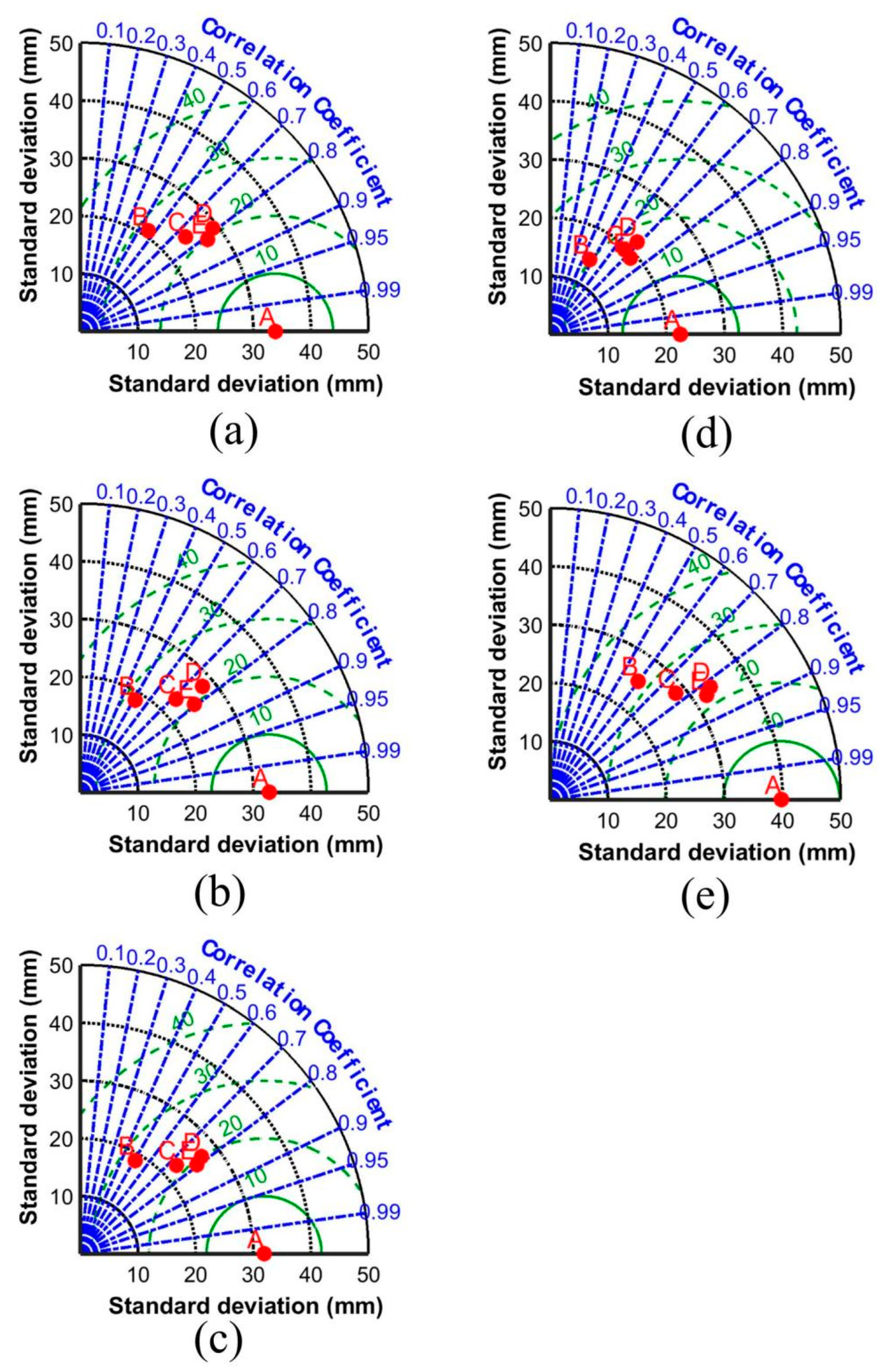
Figure 6 shows the Taylor diagram of various satellite products and observations. The Taylor diagram is a graphical method for evaluating the similarity between model simulation results and observation data, which was proposed by Talor in 2001. It compares multiple simulation results and observation data on a two-dimensional plane to evaluate their similarities and differences in multiple statistical indicators, such as the correlation coefficient, the standard deviation, and the root mean square error, and helps us understand the advantages and disadvantages of the model simulation results and their performance under different statistical indicators. Figure 6 is a comprehensive evaluation of all records from 2014 to 2017 and the IMERG (letter B), STEP (letter C), GWR, and RF (letter E) products. In the figure, A represents the observation data, and the closer to the actual situation (letter A) the other products (letters B to E) are, the higher the accuracy. Figure 6a–e shows a consistent distribution. RF (letter E) performs best in both CC and RMSE, and its standard deviation is slightly worse than GWR (letter D), but it is still closest to reality overall. In general, the figure shows that RF is closer to the rain gauge observation data than other products, followed by GWR and STEP, while the uncorrected IMERG performs the worst.

3.3.2. Monthly Evaluation

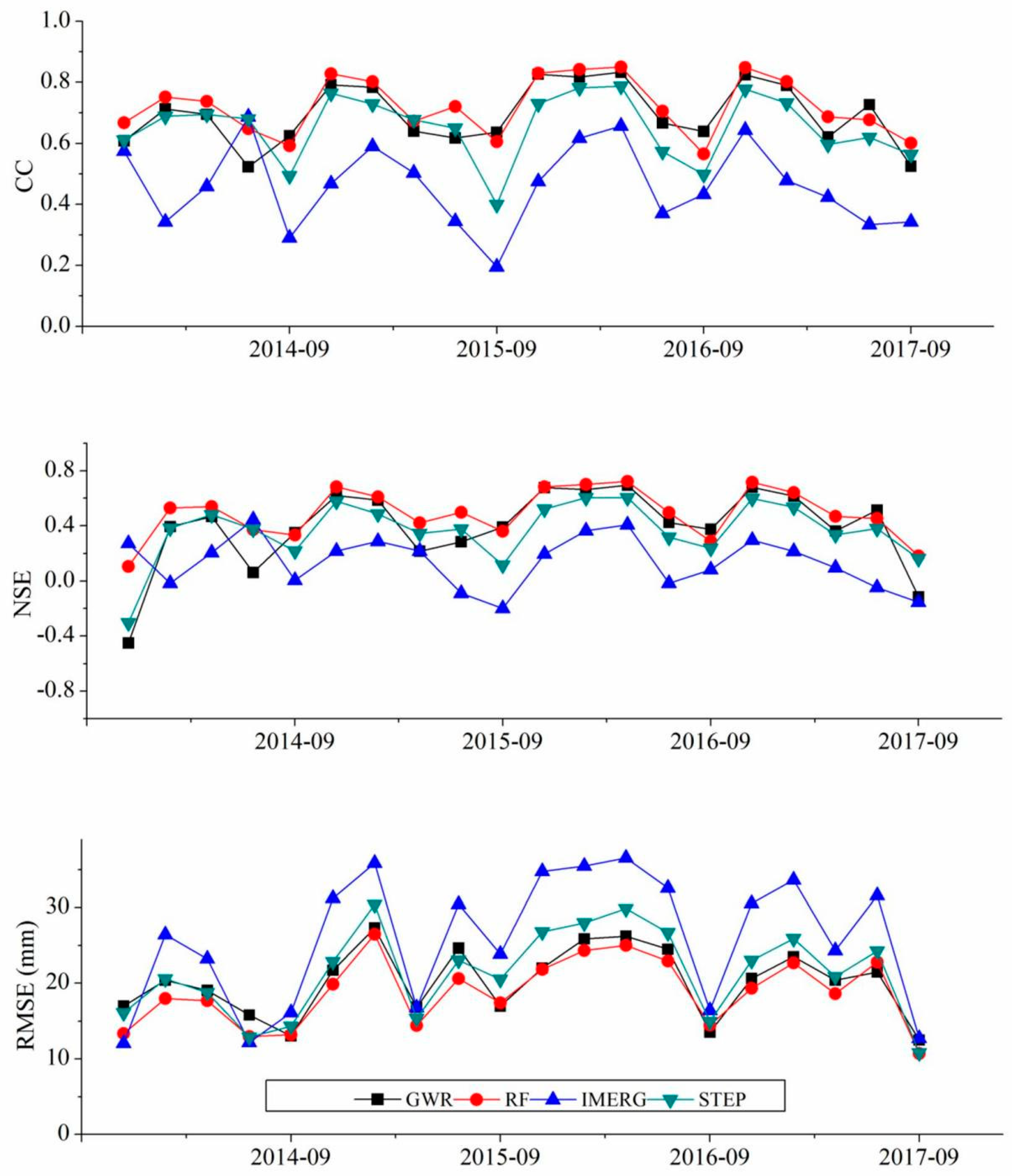
The monthly precipitation data from 2014 to 2017 in the Tianshan Mountains are counted monthly. Figure 7 shows the precipitation analysis of the original IMERG, STEP, GWR, and RF based on the rain gauge. The time variation curves of various evaluation indicators of the four precipitation products intuitively reflect that the RF precipitation quality performs best in all precipitation products at most time points. For example, CC increased from 0.20–0.69 before revision to 0.4–0.79 in STEP, 0.52–0.83 in GWR, and 0.56–0.85 in RF. RMSE decreased from 12.05–36.5 to 10.81–30.42 for STEP, 12.47–27.31 for GWR, and 10.68–26.48 for RF. This shows that the accuracy has been significantly improved after correction, and the RF correction effect is better.

3.4. Elevation Impact Analyses

All the sites in the Tianshan Mountains were rearranged in order of increasing altitude, ranging from −152 to 3616 m (Figure 1). For different station altitudes, Table 2 shows a comparison of the CC, NSE, RB, and RMSE between satellite estimates and rain gauge data at a monthly scale. For the elevation analyses, the entire Tianshan area was separated into four elevation zones: <1000, 1000–2000, 2000–3000, and >3000 m. Based on this classification, an evaluation was conducted for all the gauge stations during the warm season (May–September) from 2014 to 2017 at a monthly scale.
The CCs, NSEs, and RMSEs of the RF data were all higher than those for the other three predicted values in the first three altitude zones, while they were lower than STEP in high-altitude areas (>3000 m). One possible reason is the scarcity of sites in high-altitude areas, with fewer sites used for machine learning training. Previous studies have shown that the GWR method deteriorates to worse than STEP when sites are scarce, while this study shows that the RF method also shows its shortcomings when sites are scarce. For RB, the original IMERG data overestimated precipitation in the first two zones, but underestimated it in the last two zones. As the altitude increases, the RMSEs become larger; the maximum error occurred at elevations over 3000 m. After correction, the statistics showed that the correction method performed best for RF in areas (under 3000 m), with the best CCs and NSEs, minimum RBs, and the lowest RMSEs. For the fourth zone (over 3000 m), GWR and RF performed better than RF.

3.5. Actual Spatial Pattern of Precipitation Revealed by IMERG, STEP, GWR, and RF

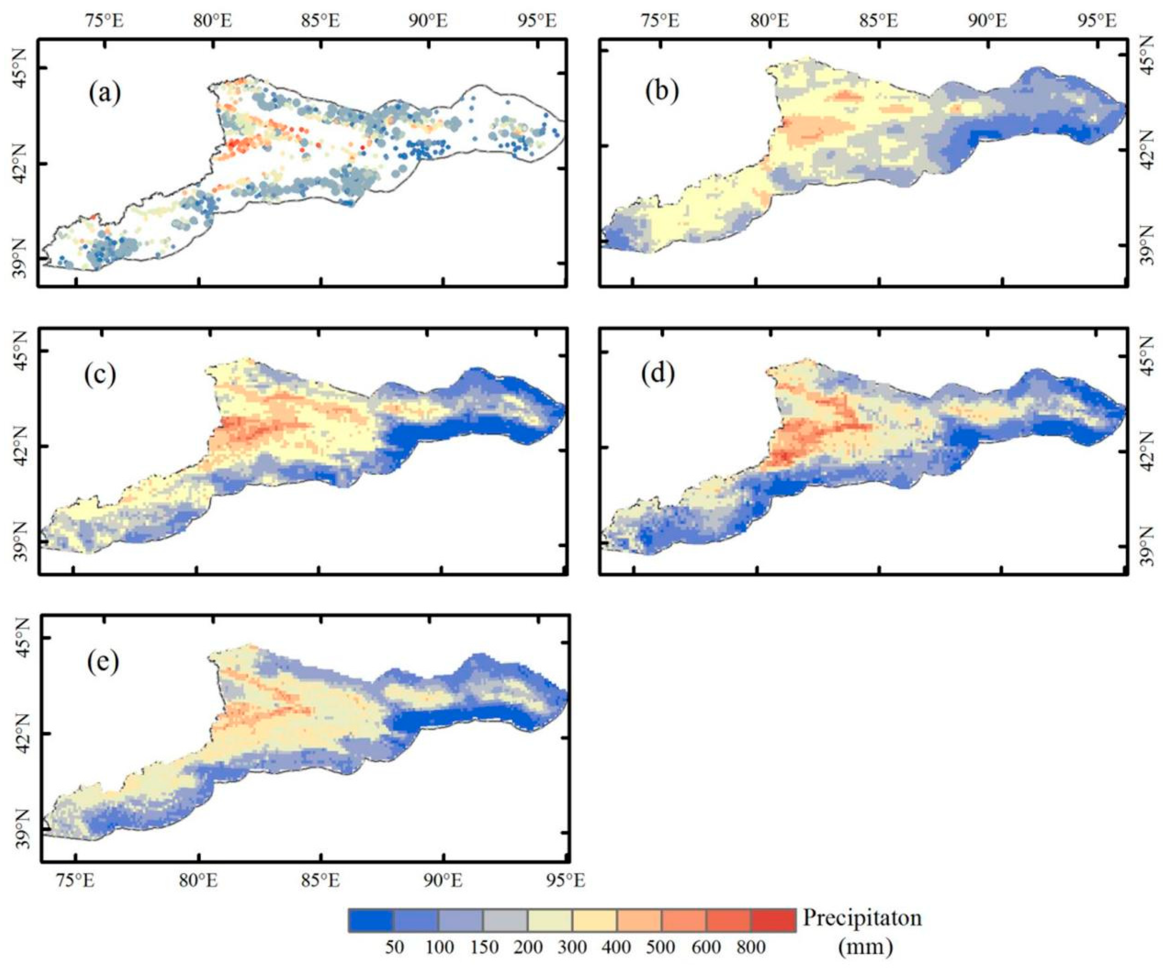
According to the statistics of the actual history of the meteorological station, 2016 was the historical maximum since the beginning of the observation of precipitation in Xinjiang over the years. Taking 2016 as an example, the topographic variables NDVI’s and IMERG’s original precipitation values of 0.1° × 0.1° grid points in the study area were first extracted and brought into the established monthly STEP, GWR, and RF models to obtain the grid data of total precipitation of 0.1° × 0.1° from May to September 2016 in the Tianshan Mountains corrected by STEP, GWR, and RF. Figure 8a is the precipitation distribution map of the live station. To facilitate comparison, the color configuration is consistent with the four grid precipitation (Figure 8b–e). The precipitation distribution of the four estimated products is consistent in the overall trend, and the large precipitation areas are concentrated in the Yili River Valley. Since the terrain of the Yili River Valley is surrounded by mountains on three sides, the branch and main vein of the Tianshan Mountains constitute a bell-shaped terrain opening to the west. The weather system in the westerly belt develops and strengthens and produces a strong precipitation process due to the blocking and lifting of the bell mouth terrain during the eastward movement, so that the western Tianshan Mountains become the precipitation center of Xinjiang. At the same time, the area near the steep terrain of the Western Tianshan Mountains is also prone to secondary disasters such as floods, mudslides, and landslides after heavy rainfall. According to statistics from live stations, the annual rainfall in this region is 417.6 mm, which is the wettest area in Xinjiang. Figure 8 shows that, compared with the actual precipitation distribution (Figure 8a), the original estimated precipitation IMERG (Figure 8b) before correction showed a significant underestimation of precipitation in the Yili River Valley, while the precipitation distribution after correction using stepwise regression (Figure 8c), geographically weighted regression (Figure 8d), and random forest (Figure 8e) was significantly improved. Since the live stations are still sparse, the surface rainfall generated by the live interpolation method will bring large errors, we can only use the existing discrete stations to compare and evaluate satellite precipitation. Through further statistics, the average precipitation of the four estimation products (IMERG, STEP, GWR, and RF) in the whole study area from May to September in 2016 was 184, 190, 195.1, and 206.9 mm, respectively. While the average precipitation measured at the live site in the same period was 211.3 mm, RF was closest to the live value, and the IMERG, STEP, and GWR underestimated by 12.9%, 10.1%, and 7.7%, respectively. From the perspective of standard deviation, the actual precipitation and IMERG, STEP, GWR, and RF were 149.2, 76.03, 108.3, 110.2, and 140.9, respectively. Therefore, IMERG, STEP, and GWR were 49%, 27%, and 26% smaller than the actual precipitation, respectively, while the RF was comparable to the actual precipitation. Based on the above analysis results, the initial GPM IMERG underestimated the heavy rainfall and was significantly improved after RF correction. These results also suggest that RF products are more reliable than the other three studies.

4. Discussion

Precipitation in mountainous areas is the most important link in the hydrological cycle of arid areas and an important source of water resources. The complex terrain in mountainous areas affects the accuracy of precipitation inversion. We studied the correction of original satellite precipitation by selecting different methods, among which the traditional STEP linear regression belongs to the global model. Due to the use of fixed coefficients throughout the entire operation process, it is assumed that the relationship between variables is “homogeneous” before analysis, and the results obtained are only a certain “average” within the study area. GWR has advantages in exploring the spatial variation relationships between variables and predicting future results by establishing local regression equations at each point within the spatial range. However, GWR also has a drawback, which is that it cannot automatically remove input variables with poor correlation like stepwise regression due to the influence of the selected independent variables. Therefore, the selection of independent variables is particularly important when using the GWR method. The selection of prediction factors is a key step in correcting satellite precipitation data. By analyzing and screening the characteristics of the dataset, we can identify factors that have a significant impact on the predicted target. Common predictor screening methods include univariate statistical analysis, multivariate statistical analysis, and machine learning algorithms. These methods can select indicators according to different features, and classify and filter features to improve the accuracy and stability of the prediction model. RF provides an effective method, that is feature engineering, to select relevant features from a dataset. Feature engineering is a process of obtaining more information by sorting and combining feature variables. Different from the previous models constructed by manually screening variables through a large amount of data analysis, RF provides a method to acquire knowledge from data and can gradually improve the performance of the prediction model and apply the model to data-driven decision-making. Therefore, feature engineering can screen out an effective combination of explanatory factors from a large amount of remote sensing data to achieve an accurate and fine estimation of precipitation in data-deficient areas. The importance of features is measured by the average impure attenuation of all decision trees in the RF, regardless of whether the data is linearly separable. In addition, unlike previous methods of manually deriving rules and building models through extensive data analysis, RF provide a way to obtain knowledge from data while gradually improving the performance of predictive models and applying them to data-driven decision-making. RF is famous for its ability to deal with complex nonlinear relationships between variables while minimizing the over fitting problem. Due to its good generalization ability, scalability, ease of use, and other characteristics, RF has received extensive attention in the field of machine learning applications in the past decade.

5. Summary and Conclusions

In this study, the terrain factor and vegetation index were introduced as independent variables, and the actual precipitation was used as the dependent variable. Stepwise regression and geographically weighted regression were selected as correction methods to study the satellite precipitation correction technology in the Tianshan Mountains of Xinjiang. The distribution of precipitation in mountainous areas is very complex and is not only related to climatic conditions, but it is also affected by topography and altitude. For many years, the influence of geographical and topographic factors on the distribution of precipitation has been discussed by academia and application departments [14,17,30,31]. Therefore, this study selected widely used terrain factors for the calibration of satellite precipitation products. Vegetation coverage has a good indication effect on precipitation. Among the many vegetation indexes, the NDVI is one of the most widely used. Because the surface of the Tianshan Mountains in Xinjiang is mostly covered with snow in winter and the vegetation has stopped growing, the time range of this study was selected to be from May to September in the warm season, which is also consistent with the fact that the regional live station can only observe the warm season precipitation.
There is still a problem where the effective explanatory factors cannot be fully utilized in the use of correction methods to further improve the quality of satellite precipitation products. The wide application of machine learning provides a powerful tool for extracting auxiliary variables closely related to precipitation in massive observation data. In machine learning, these explanatory factors or auxiliary variables are called feature variables, and the screening process for these feature variables is called feature engineering. Among the many machine learning algorithms, RF is known for its ability to address complex nonlinear relationships between variables while minimizing overfitting problems and not being affected by multicollinearity. Due to their good generalization ability, prediction performance, scalability, and ease of use, random forests have received extensive attention over the past decade.
STEP, GWR, and RF can improve the quality of IMERG products in the Tianshan area of Xinjiang with complex terrain and sparse live stations, and the correction effects of the GWR and RF methods is more significant. Therefore, it can be used as a practical method to improve the accuracy of satellite precipitation products in this study area. Although the study area is the Tianshan Mountains in Xinjiang, the calibration method can be applied to other mountainous regions of the world, and meteorological and hydrological researchers can obtain more accurate results by correcting precipitation. In addition, this study takes the monthly precipitation data of GPM IMERG as the research object. Considering the requirements for high temporal resolution precipitation data in weather forecasting and hydrological simulation, future research should focus on the correction of satellite precipitation products at daily or even hourly scales, which is more challenging.

Author Contributions

Conceptualization, X.L. and Y.L. (Yan Liu); methodology, Y.L. (Yan Liu); software, J.L.; validation, Y.L. (Yang Li); formal analysis, J.L.; investigation, H.H.; resources, X.L.; data curation, H.H.; writing—original draft preparation, X.L.; writing—review and editing, Y.L. (Yang Li); visualization, X.L.; supervision, Y.L. (Yan Liu); project administration, Y.L. (Yan Liu); funding acquisition, X.L. and J.L. All authors have read and agreed to the published version of the manuscript.

Funding

This research was funded by the Basic Research Operating Expenses of the Central Level Nonprofit Research Institutes (IDM2020006), State Key Laboratory of Cryospheric Science, Northwest Institute of Eco-Environment and Resources, Chinese Academy Sciences (SKLCS-OP-2021-10), the National Natural Science Foundation of China (42071075), the Fengyun Application Pioneering Project (FY-APP-2022.0401), and the S&T Development Fund of IDM (KJFZ202305).

Acknowledgments

We are grateful to the scientists on the NASA science team for providing satellite precipitation and DEM data. We thank the Xinjiang Meteorological Information Center for providing the gauge-observed precipitation data.

Conflicts of Interest

The authors declare no conflict of interest.

References

  1. Yi, L.; Gao, Z.; Shen, Z.; Lin, H.; Liu, Z.; Ma, S.; Wang, C.; Li, S.; Li, L. Precipitation Estimation Based on Infrared Data with a Spherical Convolutional Neural Network. J. Hydrometeor. 2023, 24, 743–760. [Google Scholar] [CrossRef]
  2. Ji, Q.; Yan, S.; He, Y.; Lu, X.; Ma, Z. Spatio-temporal patterns of snow cover in the Tien Shan, China from 2000 to 2019 based on cloudfree data supported by Google Earth Engine. Remote Sens. Lett. 2023, 14, 265–276. [Google Scholar] [CrossRef]
  3. Tang, G.; Ma, Y.; Long, D.; Zhong, L.; Hong, Y. Evaluation of GPM Day-1 IMERG and TMPA Version-7 Legacy Products over Mainland China at Multiple Spatiotemporal Scales. J. Hydrol. 2016, 533, 152–167. [Google Scholar] [CrossRef]
  4. Lu, X.; Tang, G.; Wei, M.; Yang, L.; Zhang, Y. Evaluation of multi-satellite precipitation products in Xinjiang, China. Int. J. Remote Sens. 2018, 39, 7437–7462. [Google Scholar] [CrossRef]
  5. Ma, Z.; Xu, J.; Ma, Y.; Zhu, S.; He, K.; Zhang, S.; Ma, W.; Xu, X. AERA5-Asia: A Long-Term Asian Precipitation Dataset (0.1°, 1-Hourly, 1951–2015, Asia) Anchoring the ERA5-Land Under the Total Volume Control by APHRODITE. Bull. Am. Meteorol. Soc. 2022, 103, E1146–E1171. [Google Scholar] [CrossRef]
  6. Shi, Y.; Sun, Z.; Yang, Q. Characteristics of area precipitation in Xinjiang region with its variations. J. Appl. Meteorol. Sci. 2008, 19, 326–332. (In Chinese) [Google Scholar]
  7. Chen, Y.; Li, Z.; Fang, G.; Deng, H. Impact of climate change on water resources in the Tianshan Mountians, Central Asia. Acta Geo. Sin. 2017, 1, 18–26. (In Chinese) [Google Scholar]
  8. Huffman, G.J.; Bolvin, D.T.; Braithwaite, D.; Hsu, K.; Joyce, R.; Kidd, C.; Nelkin, E.J.; Xie, P. NASA Global Precipitation Measurement (GPM) Integrated Multi-Satellite Retrievals for GPM (IMERG) Algorithm Theoretical Basis Document (ATBD) Version 4.5. 2017. Available online: http://pmm.nasa.gov/sites/default/files/document_files/IMERG_ATBD_V5.1b (accessed on 1 August 2022).
  9. Huffman, G.J.; Bolvin, D.T.; Nelkin, E.J. Integrated Multi-Satellite Retrievals for GPM (IMERG) Technical Documentation. 2017. Available online: http://pmm.nasa.gov/sites/default/files/document_files/IMERG_doc_171117b.pdf (accessed on 1 August 2022).
  10. Immerzeel, W.W.; Rutten, M.M.; Droogers, P. Spatial downscaling of TRMM precipitation using vegetation response on the Iberian Peninsula. Remote Sens. Environ. 2009, 113, 362–370. [Google Scholar] [CrossRef]
  11. Jia, S.; Zhu, W.; Lu, A.; Yan, T. A statistical spatial downscaling algorithm of TRMM precipitation based on NDVI and DEM in the Qaidam Basin of China. Remote Sens. Environ. 2011, 115, 3069–3079. [Google Scholar] [CrossRef]
  12. Xu, S.; Wu, C.; Wang, L.; Gonsamo, A.; Shen, Y.; Niu, Z. A new satellite-based monthly precipitation downscaling algorithm with non-stationary relationship between precipitation and land surface characteristics. Remote Sens. Environ. 2015, 162, 119–140. [Google Scholar] [CrossRef]
  13. Warren, S.D.; Hohmann, M.G.; Auerswald, K.; Mitasova, H. An evaluation of methods to determine slope using digital elevation data. Catena 2004, 58, 215–233. [Google Scholar] [CrossRef]
  14. Yin, Z.; Liu, X.; Zhang, X.; Chung, C. Using a geographic information system to improve Special Sensor Microwave Imager precipitation estimates over the Tibetan Plateau. J. Geophys. Res. 2004, 109, D03110. [Google Scholar] [CrossRef] [Green Version]
  15. Chen, S.; Hong, Y.; Cao, Q.; Gourley, J.J.; Kirstetter, P.E.; Yong, B. Similarity and difference of the two successive v6 and v7 TRMM multisatellite precipitation analysis performance over China. J. Geophys. Res.-Atmos. 2013, 118, 13060–13074. [Google Scholar] [CrossRef]
  16. Sørensen, R.; Seibert, J. Effects of DEM resolution on the calculation of topographical indices: TWI and its components. J. Hydrol. 2007, 347, 79–89. [Google Scholar] [CrossRef]
  17. Yin, Z.; Zhang, X.; Liu, X.; Colella, M.; Chen, X. An assessment of the biases of satellite rainfall estimates over the Tibetan Plateau and correction methods based on topographic analysis. J. Hydrometeor. 2008, 9, 301–326. [Google Scholar] [CrossRef]
  18. Shen, Y.; Pan, Y.; Yu, J.; Zhao, P.; Zhou, Z. Quality assessment of hourly merged precipitation product over China. Trans. Atmos. Sci. 2013, 36, 37–46. (In Chinese) [Google Scholar] [CrossRef]
  19. Ma, L.; Zhang, T.; Frauenfeld, O.; Ye, B.; Yang, D.; Qin, D. Evaluation of precipitation from the ERA-40, NCEP-1, and NCEP-2 reanalysis and CMAP-1, CMAP-2, and GPCP-2 with ground-based measurements in China. J. Geophys. Res. 2009, 114, D09105. [Google Scholar] [CrossRef]
  20. Ward, E.; Buytaert, W.; Peaver, L.; Wheater, H. Evaluation of precipitation products over complex mountainous terrain: A water resources perspective. Adv. Water Resour. 2011, 34, 1222–1231. [Google Scholar] [CrossRef]
  21. Blacutt, L.; Herdies, D.; Goncalves, L.; Vila, D.; Andrade, M. Precipitation comparison for the CFSR, MERRA, TRMM3B42 and combined scheme datasets in Bolivia. Atmos. Res. 2015, 163, 117–131. [Google Scholar] [CrossRef] [Green Version]
  22. Hu, Z.; Hu, Q.; Zhang, C.; Chen, X.; Li, Q. Evaluation of reanalysis, spatially-interpolated and satellite remotely-sensed precipitation datasets in Central Asia. J. Geophys. Res. 2016, 121, 5648–5663. [Google Scholar] [CrossRef] [Green Version]
  23. Beale, E.M.L.; Kendall, M.G.; Mann, D.W. The discarding of variables in multivariate analysis. Biometrika 1967, 54, 357–366. [Google Scholar] [CrossRef] [PubMed]
  24. Newton, R.G.; Spurrell, D.J. A development of multiple regression for the analysis of routine data. Appl. Stat. 1967, 16, 51–64. [Google Scholar] [CrossRef]
  25. Brunsdon, C.; Fotheringham, A.S.; Charlton, M.E. Geographically weighted regression: A method for exploring spatial nonstationarity. Geogr. Anal. 1996, 28, 281–298. [Google Scholar] [CrossRef]
  26. Fotheringham, A.S.; Brunsdon, C.; Charlton, M. Geographically Weighted Regression: The Analysis of Spatially Varying Relationships; Wiley: Hoboken, NJ, USA, 2002; 282p, ISBN 978-0-471-49616-8. [Google Scholar]
  27. Propastin, P.; Kappas, M.; Erasmi, S. Application of geographically weighted regression to investigate the impact of scale on prediction uncertainty by modelling relationship between vegetation and climate. Int. J. Spat. Data Infra. Res. 2008, 3, 73–94. [Google Scholar]
  28. Kalra, A.; Ahmad, S. Estimating annual precipitation for the Colorado River Basin using oceanic-atmospheric oscillations. Water Resour. Res. 2012, 48, 313–325. [Google Scholar] [CrossRef] [Green Version]
  29. Gupta, S.A.; Tarboton, D.G. A tool for downscaling weather data from large-grid reanalysis products to finer spatial scales for distributed hydrological applications. Environ. Model. Softw. 2016, 84, 50–69. [Google Scholar] [CrossRef] [Green Version]
  30. Yang, Y.; Luo, Y. Using the back propagation neural network approach to bias correct TMPA data in the arid region of North-west China. J. Hydrometeor. 2014, 15, 459–473. [Google Scholar] [CrossRef] [Green Version]
  31. Lu, X.; Tang, G.; Wang, X.; Liu, Y.; Jia, L.; Xie, G.; Li, S.; Zhang, Y. Correcting GPM IMERG precipitation data over the Tianshan Mountains in China. J. Hydrol. 2019, 575, 1239–1252. [Google Scholar] [CrossRef]
Figure 1. Distribution of altitude and annual precipitation at meteorological stations in the study area.
Remotesensing 15 03962 g001
Figure 2. The flow chart of this study.
Remotesensing 15 03962 g002
Figure 3. Importance ranking of predictive factors.
Remotesensing 15 03962 g003
Figure 4. Scatter plot of IMERG, STEP, GWR, RF, and monthly precipitation in the warm season (May–September) from 2014 to 2017 (the dotted lines represent the 1:1 lines).
Remotesensing 15 03962 g004
Figure 5. Boxplot of correlation coefficient, root mean square error, relative error, and absolute mean error of IMERG, STEP, GWR, and RF in the warm season (May–September) from 2014 to 2017.
Remotesensing 15 03962 g005
Figure 6. Taylor diagrams of the four precipitation products for (a) the whole period and (be) each year between 2014 and 2017 over the Tianshan Mountains (letters A, B, C, D, and E denote OBS, IMERG, STEP, GWR, and RF, respectively).
Remotesensing 15 03962 g006
Figure 7. Monthly variation in the correlation coefficient, root mean square error, and Nash efficiency coefficient of IMERG, STEP, GWR, and RF in the warm season (May to September) from 2014 to 2017.
Remotesensing 15 03962 g007
Figure 8. Spatial distribution of the annual precipitation from May to September 2016 over the Tianshan Mountains for (a) OBS, (b) IMERG, (c) STEP, (d) GWR, and (e) RF.
Remotesensing 15 03962 g008
Table 1. Mean values of CC, RB, and RMSE for IMERG, STEP, and GWR at the monthly timescale from May to September between 2014 and 2017 over the Tianshan Mountains.
ProductCCNSERMSE (mm)MAE (mm)RB (%)
IMERG0.560.3128.1119.437.10
STEP0.740.5522.6315.421.32
GWR0.790.6220.9413.801.12
RF0.810.6619.8112.831.06
Table 2. Statistical results for in situ measurements, IMERG, STEP, GWR, and RF in four elevation zones (Bold display of the best performing indicators in the same group).
Zone≤1000 m1000–2000 m2000–3000 m>3000 m
No. of stations28456010114
CC
 IMERG0.680.630.670.66
 STEP0.70.70.670.74
 GWR0.760.750.710.68
 RF0.770.770.710.72
NSE
 IMERG0.08−0.15−0.14−0.57
 STEP0.290.30.19−0.04
 GWR0.430.420.21−0.31
 RF0.480.480.29−0.09
RB (%)
 IMERG31.13.13−32.6−38.49
 STEP7.09−0.911.128.85
 GWR2.370.42−3.7−11.49
 RF0.91−0.150.73−13.4
RMSE (mm)
 IMERG19.2830.0634.4439.68
 STEP16.9223.4728.9732.29
 GWR15.2621.2428.5636.29
 RF14.520.0927.1533.07
Disclaimer/Publisher’s Note: The statements, opinions and data contained in all publications are solely those of the individual author(s) and contributor(s) and not of MDPI and/or the editor(s). MDPI and/or the editor(s) disclaim responsibility for any injury to people or property resulting from any ideas, methods, instructions or products referred to in the content.