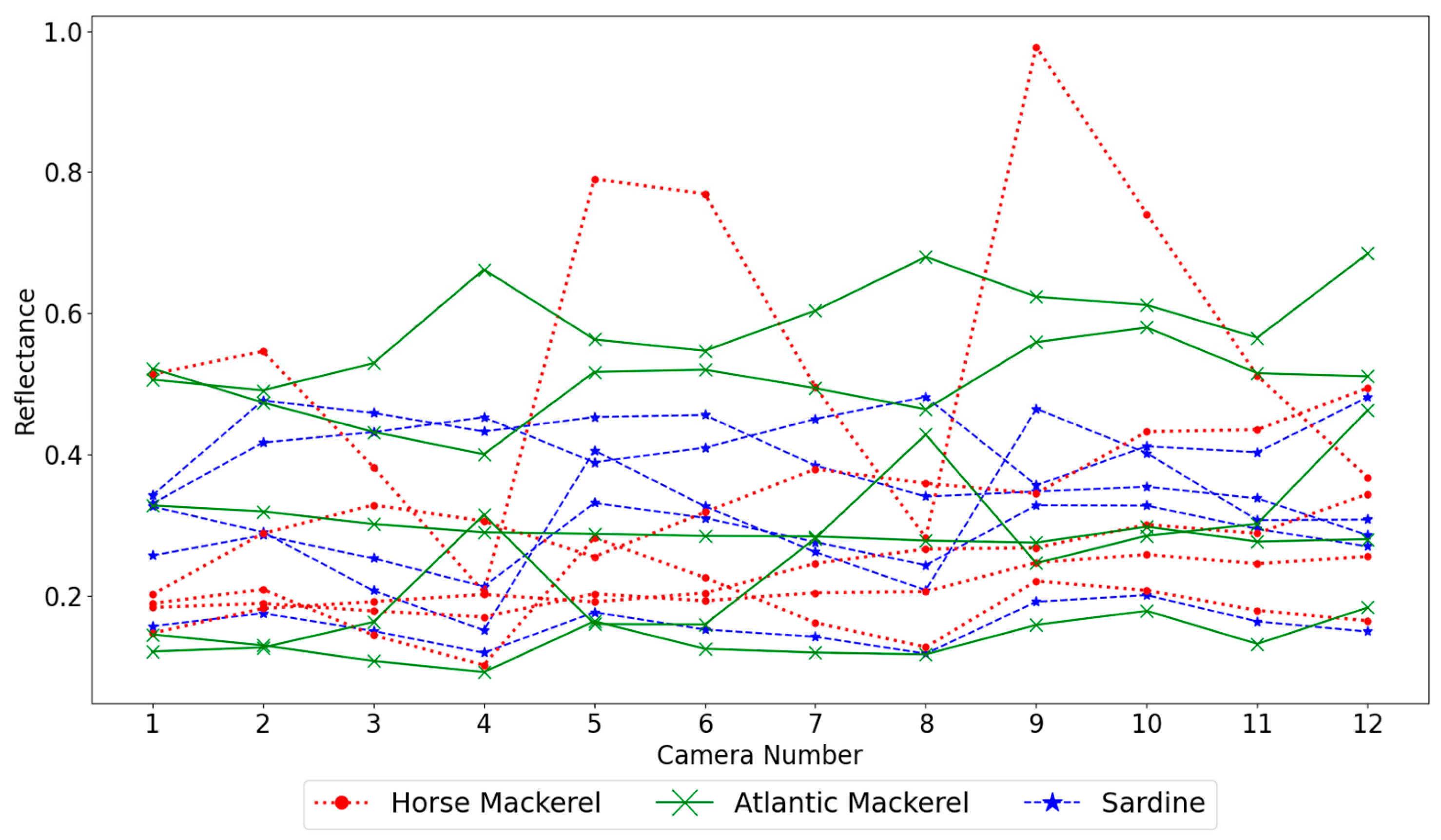
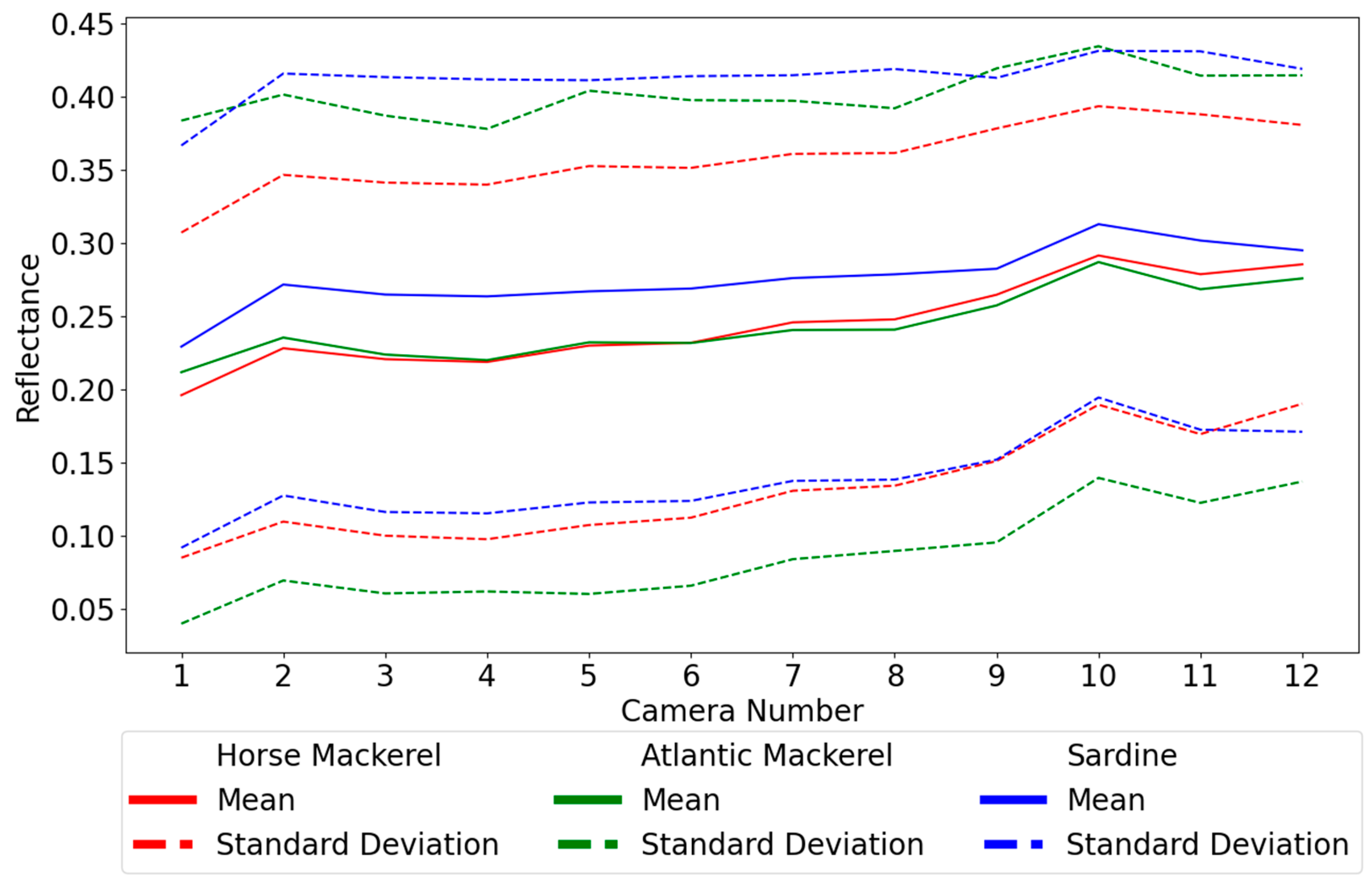
This section starts by showing the reflectance spectra and analyzing the best image resolution to create spectra for classification, followed by comparing the results for the three types of classifiers selected, KNN, MP, and SVMs. A possible selection of cameras and the impact of the white target composition and size on the results are also studied. Finally, a method is proposed to estimate the percentage of spectra from each species present in the obtained images, not only the percentage corresponding to true detections plus false positives of another species but an overall approach considering the misdetections of each species. All calculations were performed in Windows 11 and Python 3.10.7 on an i7-11700@2.5 GHz machine with eight cores and 16 MB of RAM. The machine learning algorithms are from Sklearn, version 1.1.3.
3.2. Image Resolution Downscaling Effect
Pixel-wise analysis of the images resulted in an extensive dataset with a high correlation between neighboring pixels. This high correlation allows the application of a downscaling step to the data without significant loss of the overall information present in the dataset. The downsample averaging was processed by sweeping an N × N mask, without overlapping, through the images, averaging the spectra of the pixels. The tested masks were squares whose sides had an odd number of pixels, ranging from 3 × 3 to 15 × 15. The main benefit of this downscaling step is that it reduces the variance of the resulting average spectra as the mask size increases. An additional benefit is a decrease in the computational cost of the training processes since downsampling results in a much smaller dataset than the original set. Too much downscaling may destroy the features required for proper classification.
The trained models used hyperparameters that were reasonable according to preliminary tests. KNN uses neighborhoods composed of five elements with a uniform weight function; the MP comprises two hidden layers of twenty and ten neurons employing an Adam solver for weight optimization with an initial learning rate of 0.002; and SVM uses a regularization parameter of one. The results for all models are organized in
Table 1, where the balanced accuracies are given for different pixel neighborhood sizes.
The best pixel neighborhood size for downsampling for SVM is 5 × 5 by at least 0.4 percentage points (p.p.), relative to the second best. For MP, the value of 7 × 7 is the best but only with a difference of 0.1 p.p. for 5 × 5. With KNN, the best option is 1 × 1. At this point, it was necessary to choose if one would select the best value for each algorithm, leading to considerable variation in the reflectances being input into the algorithms. To avoid this, the same downsampling was used for all algorithms. The value of 5 × 5 seems adequate for at least MP and SVM. Even though it is not the best for the former, it still leads to better results than for SVM. For KNN, 5 × 5 still provides good results since the decay is not very pronounced. When performing a downscaling with a 5 × 5 mask, one obtains a dataset at least 25 times smaller than the original set while maintaining the quality of information. The downscaled dataset contains 20,473, 15,653, and 12,615 spectra for horse mackerel, Atlantic mackerel, and sardines. Comparing batches one and two, as shown in
Table 2, indicates that the latter has more spectra for all species. The increases for horse and Atlantic mackerel are 31% and 25%, respectively, but the number more than doubles for sardines.
3.3. Hyperparameter Optimization
After establishing the downsampling, the hyperparameters were thoroughly optimized. For KNN, several models with various-sized neighborhoods, 5, 10, 20, 40, 80, 160, and 320, were trained and tested with the value of 20 returning good results. For MP, the configurations tested consisted of a single hidden layer with 6, 10, 20, 30, 40, 50, 60, and 70 neurons and two layers where the first had 8, 12, 20, 30, 40, 50, 60, and 70 neurons with the second layer containing half the number of neurons of the first layer. Using two hidden layers with 60 and 30 nodes was the best option. The neural model can use the Adam solver to adjust the learning rate with each epoch of the training process or the stochastic gradient descent solver with a constant learning rate. Models with each solver and with various initial learning rates, namely 0.001, 0.01, 0.1, 1, and 10, were trained to find the best solver and initial learning rate. Models tested with the Adam solver showed that the desired initial learning rate lies between 0.001 and 0.01. Further testing with learning rates between 0.001 and 0.01, with a step of 0.001, resulted in the best value of 0.004. Models tested with the SGD solver showed that the desired initial learning rate lies between 0.01 and 0.1. Further testing between those values resulted in the best value of 0.015. The best models scored balanced accuracies of 63.8% and 64.4% with the Adam solver and SGD, respectively. For SVM, the analyzed values of the regularization parameter were between 1 × 10⁻⁴ and 1 × 10⁴, varying in powers of ten. The balanced accuracy steadies after a regularization parameter of 1000, making this value a good choice.
3.4. Tuned Classifier Comparison
Three classifiers, the best from each algorithm, are compared using confusion matrices, balanced accuracy, and training time.
Table 3 shows balanced accuracies and training times.
The balanced accuracies for KNN, MP, and SVM are 56.7%, 64.4%, and 65.3%, respectively. Although smaller than one would like, these values are far from the 33% expected for a random three-class classifier, confirming that the data have enough information to separate the classes. The training times are, in the same order as before, 1 s, 3 min and 2 s, and 8 h, 29 min, and 36 s. SVM, the best classifier, presents the most considerable training time. Nevertheless, one must note that the classification with SVM is significantly faster than its training.
Table 4 shows the confusion matrices of the classifier’s predictions for ten-fold cross-validation.
For KNN, the sardine spectra’s true positive percentage is 62.5%, significantly above the horse and Atlantic mackerel’s true positive percentages of 50.7% and 56.9%, respectively. While the sardine spectra’s incorrect classifications are split relatively evenly between the other species, with 18.5% and 18.9% for horse and Atlantic mackerel, respectively, the horse and Atlantic mackerel spectra are incorrectly classified as each other at a slightly higher percentage than as sardines. KNN incorrectly classified horse mackerel spectra at 25.6% and 23.7% rates as Atlantic mackerel and sardines, respectively, and Atlantic mackerel spectra at 22.8% and 20.4% as horse mackerel and sardines, respectively.
The correct classifications/true positive percentages for the MP are 61.2%, 60.3%, and 71.7% for horse mackerel, Atlantic mackerel, and sardines, respectively. Incorrect classifications of sardine spectra are split evenly between horse and Atlantic mackerel but at a lower percentage than with the KNN, at 14.2 and 14.1%. MP classifies horse mackerel spectra as Atlantic mackerel and sardines at 22.2% and 16.6%, while the Atlantic mackerel spectra’ corresponding percentages are 24.0% and 15.7% for horse mackerel and sardines.
SVM true positive percentages are 65.5%, 58.9%, and 71.5% for horse mackerel, Atlantic mackerel, and sardines, respectively. SVM classification of horse mackerel is better than with the other two classifiers, and it is slightly worse for sardines than MP but substantially better than KNN. There is a 1.4 p.p. decrease with SVM for Atlantic mackerel compared to MP and a 2 p.p. increase compared to KNN. Horse mackerel classification with SVM is 4.3 and 14.8 p.p. larger than with MP and KNN, respectively. The SVM classifies sardines incorrectly as horse mackerel more than as Atlantic mackerel, with 15.6% and 12.9%, respectively, as opposed to other models, which misclassified sardines more evenly between the other two classes. As before, horse and Atlantic mackerel spectra are incorrectly classified as each other more so than as sardines, with 19.0% and 15.5% of horse mackerel spectra classified as Atlantic mackerel and sardines, and 25.4% and 15.7% of Atlantic mackerel spectra classified as horse mackerel and sardines, respectively. With SVM, compared to MP, the decrease in 1.4 and 0.2 p.p. of the Atlantic mackerel’s and sardines’ true positive percentages is compensated for by the better results for horse mackerel. All classifiers show a higher discernment for sardines than any other species.
3.5. Models Classification Trust
This section analyses the outcome of the best SVM created. While a significant percentage of classifications are correct, the certainty of those classifications varies significantly between species and locations on the fish body. For each spectrum, the classifier determines the probability of that spectrum being from a horse mackerel, an Atlantic mackerel, or a sardine. Calculating the difference between the correct class probability and the highest probability of the incorrect classes returns a value indicating the strength of the decision. This difference shows how far from, or how close the classifier was to the correct prediction.
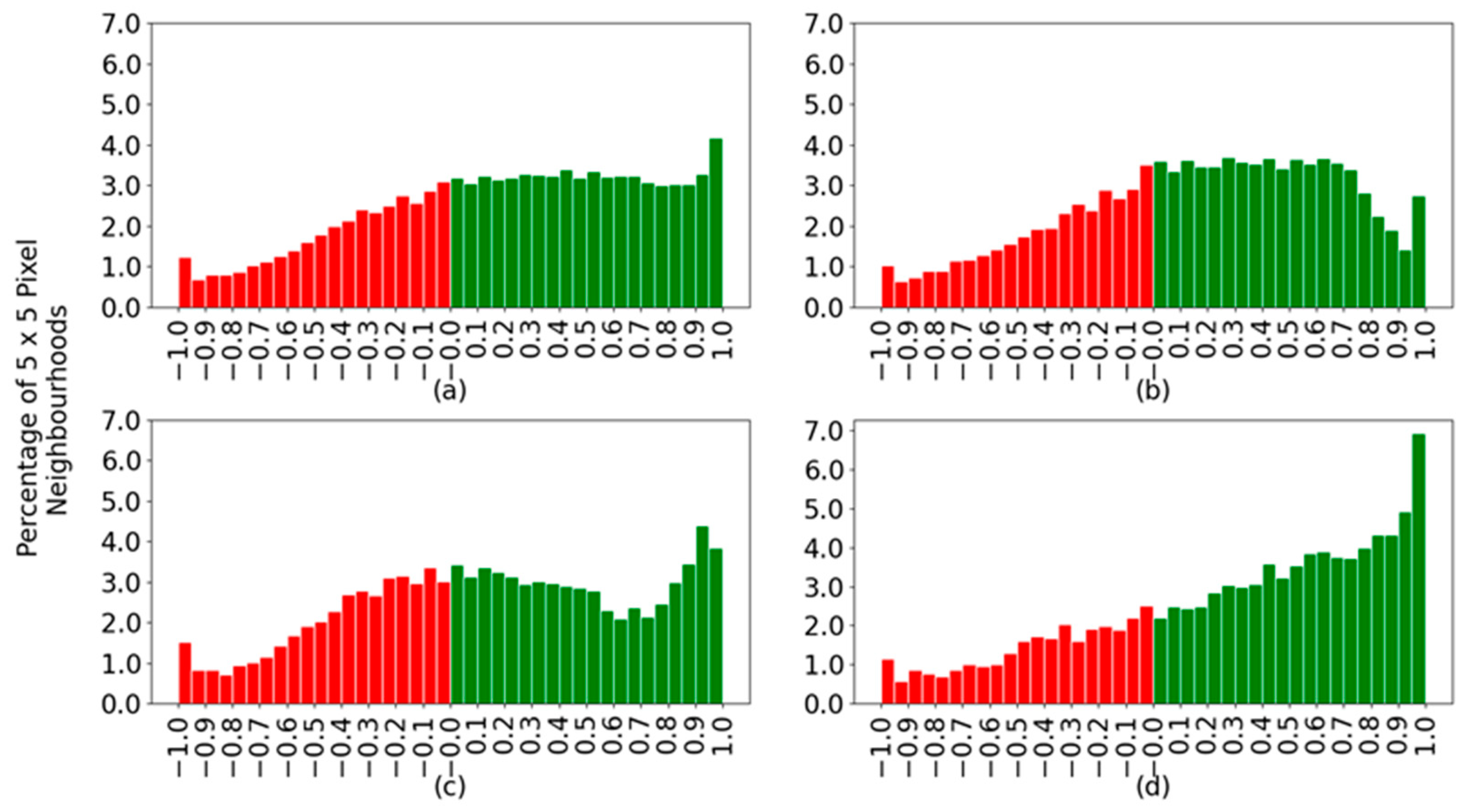
Figure 9 shows histograms created by applying the described difference of probabilities to all spectra. Positive values indicate correctly classified spectra, shown in green, and negative values correspond to incorrectly classified spectra, shown in red. The histograms contain data from all spectra together and separated by species.
Figure 9a indicates that the correctly classified spectra in green spread across the range of possible confidence values between zero and one, with a slight peak at the highest confidence. One would like to have a single bar at the value of one. With the wrongly classified spectra, there is a decay toward the more wrongly confident values, those closer to minus one, which is good. The optimal case would be to have no red bars in the histograms. When considering each species separately, the sardines (
Figure 9d) are more confidently classified and with a good slope on the green bars towards the highest confidence values. The main difference between horse and Atlantic mackerel is that although the former has an overall better classification percentage, 65.5% in
Table 4 versus 58.9% for the latter, the Atlantic mackerel has more spectra at larger confidence values. For example, compare the size of the bar for a confidence value of 0.9 in
Figure 9b,c.
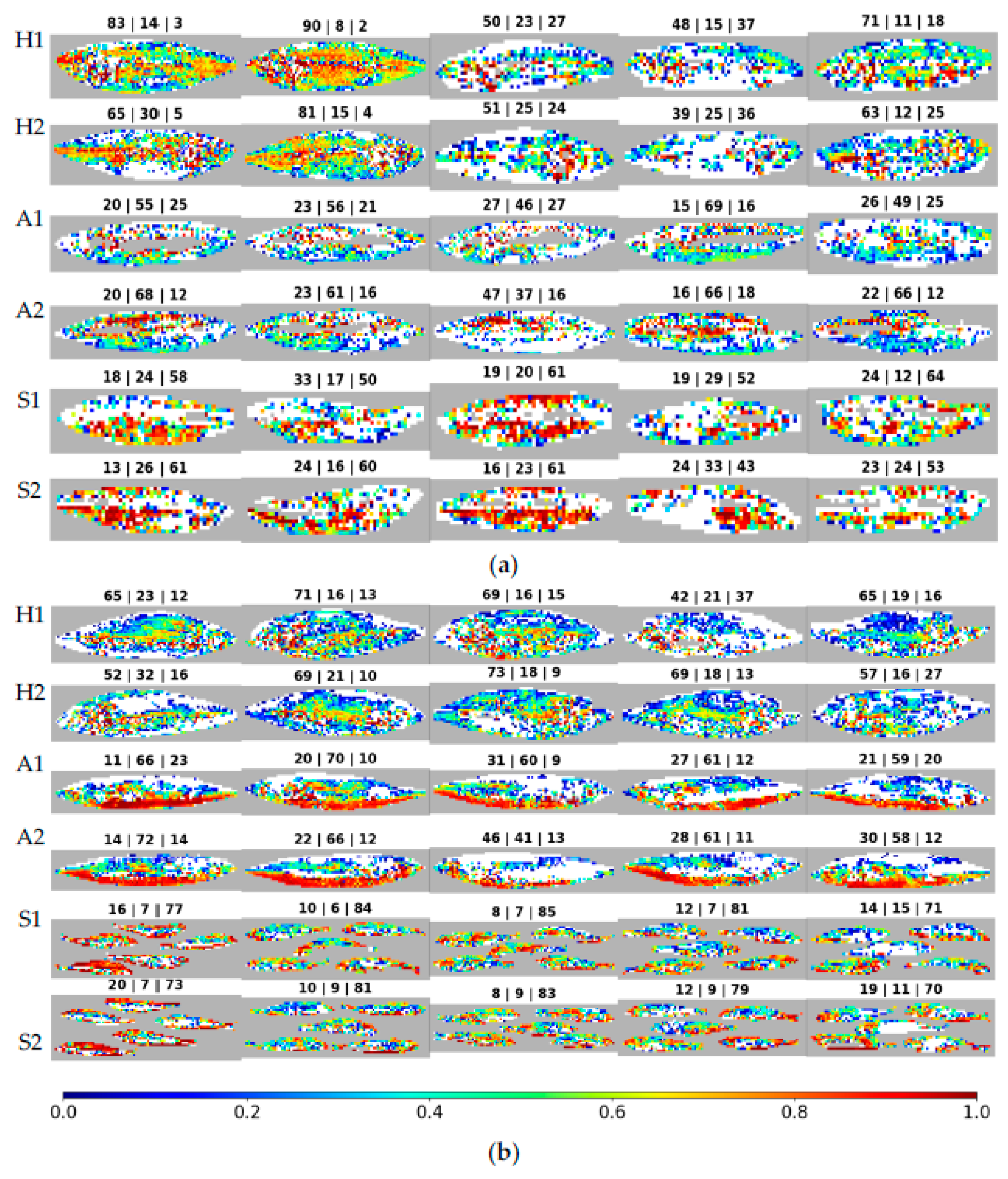
Figure 10 shows the same results as in
Figure 9 but allows one to see the distribution of correct spectra at the fish position where they come from. Image construction has the following rules: spectra that were not classified, such as ruled-out background and saturated or noise-affected spectra, are shown in grey; incorrectly classified spectra that originated the red bars in
Figure 9 are now displayed in white; and the correctly classified spectra are depicted through a color gradient based on the difference of probabilities. This difference is again between the probabilities of the correct and most probable incorrect classes. Above each image appears the percentage of spectra classified as being from each species, in the following sequence: horse mackerel, Atlantic mackerel, and sardines. The rows appear in pairs, corresponding to different sides of the same fish/fishes.
When analyzing the figure, the most striking characteristic is the tendency of various classification confidence values to show up all over the fish, visible by the colors mixing randomly. Next, the number of correctly classified spectra varies significantly, even between individuals of the same species. This characteristic is visible from the variation in the size of the white regions between various fish. It is also noticeable when analyzing the percentage of correct spectra, which is the opposite of the white spaces. The first batch’s (
Figure 10a) second horse mackerel (counting from the left) shows 90% and 81% of spectra correctly classified for each imaged side, with 8% and 15% incorrectly classified as Atlantic mackerel, showing very good discernment. Meanwhile, the first batch’s fourth sardine has 52% and 43% of spectra correctly classified, with 29% and 33% incorrectly classified as Atlantic mackerel, showing less discernment while yet classifying most spectra as the correct species. Still, in the first batch, the third Atlantic mackerel presents even worse values, with 46% and 37% of correctly classified spectra on both fish sides. Side two of this fish would be wrongly classified when using a majority vote, as the most significant number of spectra, namely 47%, are attributed to horse mackerel. When looking for differences between the first and second batches of fish, the average of correctly classified spectra, as shown in
Table 5 for horse mackerel, is 64.2% for the former and 63.3% for the latter, which are close values. With Atlantic mackerel, these values change to 57.4% and 61.4%, indicating a slightly better outcome in the second batch. For sardines, the values are 56.4% and 78.8%, with a clear advantage for the second batch.
The horse mackerels in the first batch, displayed in the first pair of rows in
Figure 10a, show differences from sample to sample, with some fish having 39% of spectra correctly classified and others having 90%. This variability is also present in the trust values, as a rainbow of colors fills the fish in
Figure 10a. Within the fish with the highest percentage of correct classifications in the first batch, the second one, the trust strength seems to be higher in the middle section of the fish and reduces as one moves away from this section. However, in the second batch, seen in the first pair of rows in
Figure 10b, the behavior is more uniform between samples. The percentage of correct classifications is between 42% and 73%, and the trust in these classifications is random but still shows slightly higher trust towards the middle section of the fish.
The Atlantic mackerels in the first batch, displayed in the second pair of rows in
Figure 10a, show discarded spectra, color-coded in grey, concentrated in the middle portion of the fish. The correctly classified spectra offer varying levels of trust seen with brown/red and blue patches clustered together in different regions of the fish, revealing no identifiable pattern and varying between samples. In the second batch, seen in the second pair of rows in
Figure 10b, a pattern emerges with the bottom half of the fish correctly classified with a high trust level, seen in brown/red. By contrast, the upper half of the fish shows a lower level of trust and more incorrect classifications, as seen in white. The percentages of correctly classified spectra vary between 37% and 69% in the first batch and between 41% and 72%, an identical variation between batches.
Lastly, sardines, displayed in
Figure 10a,b, in the last pair of rows, behave uniformly within batches but vary significantly between these batches. While the first batch of sardines has between 43% and 64% correctly classified spectra, the second batch has 70% to 85%. While the trust values vary within each fish, the overall strength of sardine classifications is usually higher than for the other species, visible by the higher presence of yellow to red/brown color-graded regions in the figure. The only exception to this trend is the Atlantic mackerel in the second batch. In the first batch, sardines have the broadest areas, between species, of fish with the highest classification confidence. Nevertheless, they do not have the greatest percentages of correctly classified spectra.
On average, as seen in
Table 5, Atlantic mackerel and sardines have the largest percentages of correctly classified spectra in the second batch. With horse mackerel, the first and second batches are only slightly different, with an advantage for the first.
3.6. Feature/Camera Selection
This section reports a study on the possibility of using less than twelve cameras to classify fish species. Tests were performed using one to twelve cameras. The results of this analysis are shown in
Table 6. The values for the KNN and MP with twelve cameras are those from
Table 3. For SVM, a slightly different gamma was used, but for twelve cameras, the result is the same as in
Table 3. The univariate feature selection generally leads to worse outcomes than the sequential feature selection (SFS) for the three types of classifiers studied. That is why some results are not given for univariate selection, and the following analysis will focus solely on SFS.
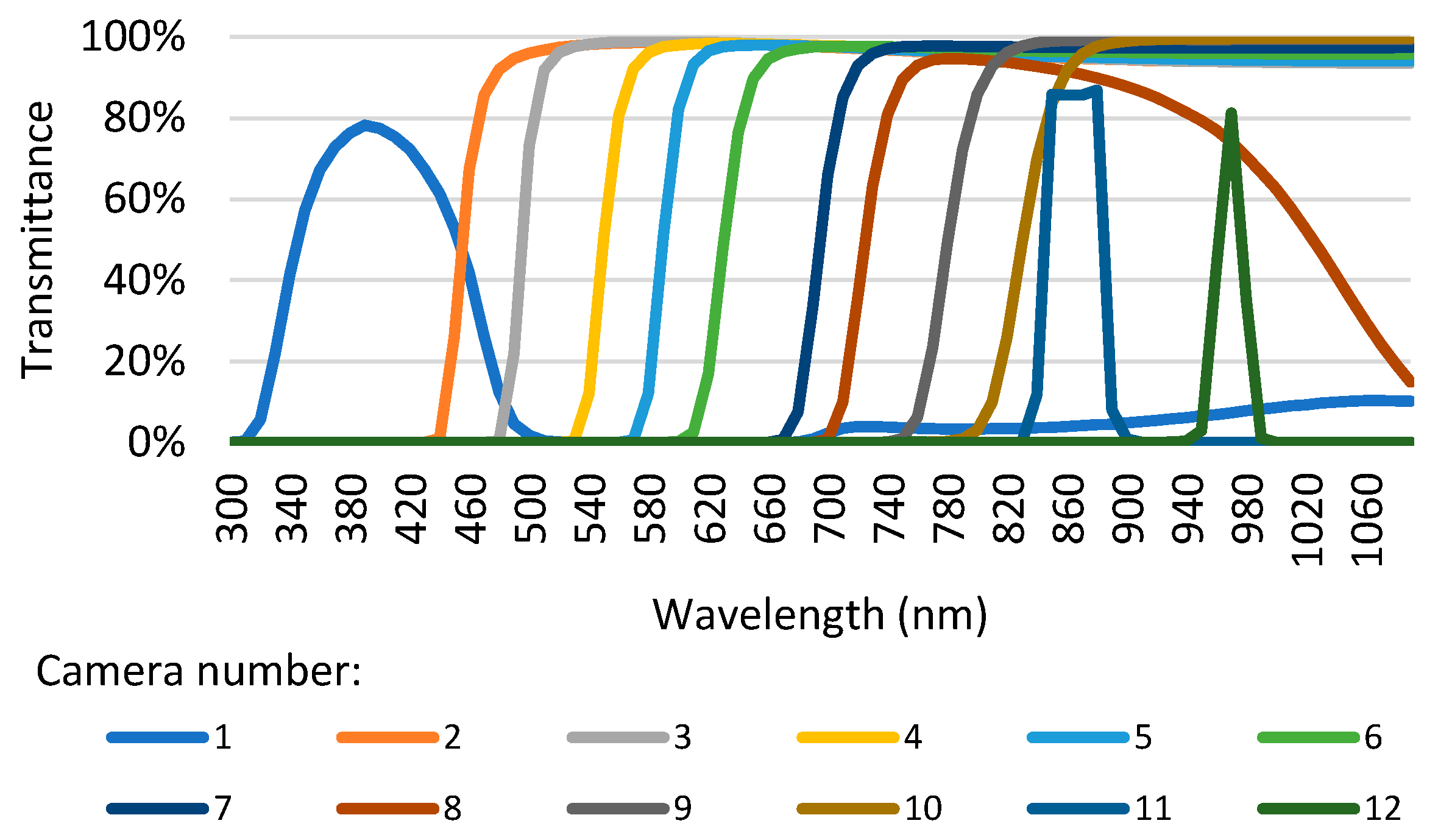
KNN returns a balanced accuracy of 56.7% using all twelve cameras. With eleven, ten, and nine cameras, one obtains improvements of 0.5, 0.7, and 0.5 p.p., respectively. The best result is achieved with ten cameras, at 57.4%. This is good since it could allow reducing the MultiCam size and cost. With six cameras, which would mean a significant downsizing, the balanced accuracy drops 1.6 p.p to 55.8%. The MP returns a balanced accuracy of 64.4% using all features. Even though the results improve when going down from eleven to eight cameras, reaching 63.3%, after that, they drop below 62%, never surpassing the case with twelve cameras. With six cameras, the balanced accuracy is 55.3%. SVM with twelve cameras shows the best results using all features, with 65.3%. However, obtaining the same balanced accuracy is possible with ten cameras, even though it means discarding cameras number 3 and 6, whose cut wavelengths are 495 nm and 630 nm, respectively, and gathering, supposedly, less information. With SVM and six cameras, the balanced accuracy drop is 6.4 p.p.
3.8. Estimation of the Number of Spectra of Each Species
The classification algorithms do not offer a 100% correct classification ability. Consequently, the direct classification results are not an immediate measure of the number of spectra available for each species in the captured images. In addition, the spectra of one species can be wrongly classified as belonging to another species. To resolve this issue, one can use the confusion matrix results to estimate the real number of spectra, considering the misclassification probabilities. With the confusion matrix given by:
| True label | Horse mackerel | | | |
| Atlantic mackerel | | | |
| Sardine | | | |
| | | Horse mackerel | Atlantic mackerel | Sardine |
| | | Predicted label |
PXY represents the probability of a spectrum of species
X being classified as being from species
Y. As previously, H, A, and S stand for horse mackerel, Atlantic mackerel, and sardines, respectively. Knowing that
QHmea,
QAmea, and
QSmea are the quantities that the classification algorithm has returned for the species, one may write:
And therefore:
where
QHorse,
QAtlantic, and
QSardine represent the real quantities of spectra of horse mackerel, Atlantic mackerel, and sardines, respectively, to be estimated in the collected images. Note that the confusion matrix is transposed. The results obtained with this method are as accurate as the statistics in creating the confusion matrix.

