Classification of Fish Species Using Multispectral Data from a Low-Cost Camera and Machine Learning

Abstract

This work creates a fish species identification tool combining a low-cost, custom-made multispectral camera called MultiCam and a trained classification algorithm for application in the fishing industry. The objective is to assess, non-destructively and using reflectance spectroscopy, the possibility of classifying the spectra of small fish neighborhoods instead of the whole fish for situations where fish are not completely visible, and use the classification to estimate the percentage of each fish species captured. To the best of the authors’ knowledge, this is the first work to study this possibility. The multispectral imaging device records images from 10 horse mackerel, 10 Atlantic mackerel, and 30 sardines, the three most abundant fish species in Portugal. This results in 48,741 spectra of 5 × 5 pixel regions for analysis. The recording occurs in twelve wavelength bands from 390 nm to 970 nm. The bands correspond to filters with the peculiarity of being highpass to keep the camera cost low. Using a Teflon tape white reference is also relevant to control the overall cost. The tested machine learning algorithms are k-nearest neighbors, multilayer perceptrons, and support vector machines. In general, the results are better than random guessing. The best classification comes from support vector machines, with a balanced accuracy of 63.8%. The use of Teflon does not seem to be detrimental to this result. It seems possible to obtain an equivalent accuracy with ten cameras instead of twelve.

1. Introduction

The seafood industry has been a considerable part of Portugal’s culture and economy for a long time [1,2]. With the goal of sustainability, caution is necessary regarding overfishing. Therefore, the continuous development of ways to monitor the fishing process is of significant importance. Information regarding a fishing ship’s intake is essential for tracking species fishing quotas to avoid overfishing and depletion of wild fisheries. Given the nature of fishing methods, each sweep of the fishing nets can contain different amounts of fish and a different number of fish species. Separating the fish by species and measuring their quantity are two steps that are currently conducted mainly through simple manual labor. The present work is the first step in automating the fish accounting per species using low-cost spectroscopy and machine learning. In the future, the system can be used inside fishing vessels or soon after fish unloading, or at the fish market.

Previous studies have applied hyper- and multispectral imaging in the seafood industry, and some use machine learning methods to extract the desired information from imaged data [3,4,5,6]. Spectroscopy allows obtaining information from recorded objects over a more comprehensive selection of wavelengths than traditional cameras that only record information for three wavelengths, the red, green, and blue wavelengths from the visual spectrum [7,8]. Since different materials and substances absorb and reflect light differently at various wavelengths, collecting this information may allow one to discern recorded objects in a non-destructive and rapid manner. The direct collection of light from objects is called reflectance spectroscopy, the method used in the present study.

Menesatti et al. [4] used partial least squares (PLS) instead of machine learning to analyze hyperspectral data; PLS is a popular and effective regression method [4,5]. Cheng and Sun [5] provided a good review of hyperspectral data to obtain information on the quality of imaged seafood, such as freshness and microbiological, physical, and chemical attributes. By contrast, the present study uses multispectral data to identify fish species. Jayasundara et al. [3] used a custom-developed multispectral camera and convolutional neural network algorithm to grade the quality of fish, which is a different purpose from ours. Their camera uses LEDs of various wavelengths instead of multiple cameras with various optical filters, which was our option. Using hyperspectral imaging methods, Kolmann et al. [6] aimed to characterize/distinguish different fish species from within the family Serrasalmidae taxonomic group. They identified and showed each species’ distinct spectrum profiles without building a species classifier. Benson et al. [9] and Ren et al. [10] used machine learning and spectroscopy to identify fish species. Ren et al. used a convolutional neural network to individually classify one-dimensional spectra—the present work also classifies spectra separately. However, Benson et al. and Ren et al. used destructive methods, the former by analyzing fish otoliths and the latter by using fish homogenates; our approach is non-destructive. Benson et al. and Ren et al. used Fourier transform, laser-induced breakdown, and Raman spectroscopy, which are more complex than reflectance spectroscopy.

The present study uses a newly developed low-cost multispectral camera, MultiCam, to record light intensity at specific wavelengths reflected from the three most fished species in Portugal, horse mackerel, Atlantic mackerel, and sardines [11,12], and applies machine learning algorithms to the recorded image’s information to discriminate the species automatically. The fish is left whole for image capture with MultiCam, making our approach non-destructive. The species separation is possible by analyzing the differences in the intensities of light reflected from the fish at the recorded wavelengths. The species are identified using small 5 × 5 pixel regions, not the whole fish image. Each of the 5 × 5 pixel regions originates a spectrum that is classified with machine learning tools. The reason for using small fish regions instead of the whole fish is to study the possibility of distinguishing overlapping fishes, which applies to fishing scenarios when the fish are still in the fishing net or soon after the fishing net’s unloading. In total, the work classifies 48,741 spectra from 5 × 5 pixel regions. To the best of the author’s knowledge, there are no reports on either reflectance spectroscopy or whole fish for species separation in the scientific literature. The use of reflectance spectroscopy is important for having low-cost equipment because the intensity of the collected signal is orders of magnitude larger than for Raman, for example.

In the long run, the authors want to use the information on the percentage of spectra of each species present in the gathered images to estimate each species’ captured amount. If the total amount of fish caught is known, the percentages of spectra of each species are all needed to calculate the amount of the individual species. To estimate the captured weight without any human intervention, one would need to have a calibration factor of the fish weight per spectra, which is outside the scope of the present article. The current article’s purpose is to start the discussion on how to proceed to estimate the percentage of spectra of each species in the gathered images. Only a non-destructive approach is useful for determining the amount of captured fish, if possible at 100%, and still commercializing the fish afterward.

The present article contains a study on which of three machine learning algorithms, k-nearest neighbors (KNN), multilayer perceptron (MP), or Support Vector Machine (SVM), is the best for fish spectra classification. It provides the confusion matrix for each case. The classification trust is reported for the best classifiers to understand the classification robustness and if it makes sense spatially. Minimizing the number of MultiCam cameras is attempted to reduce the costs of constructing MultiCam. The article also reports the possibility of using low-cost white references without loss in classification results, which is fundamental for a possible future widespread application of the developed methods. Finally, a simple method is given to estimate the number of spectra of each species considering that misclassified spectra exist but at a rate known to us.

2. Materials and Methods

2.1. Camera Description and Experimental Setup

The custom-built MultiCam (see Figure 1) comprises twelve cameras equipped with transparent filters at different wavelengths. The cameras are placed side-by-side in a 4 × 3 matrix. Figure 2 shows the transmittance of the filters for wavelengths from 300 to 1060 nm. A total of 9 cameras have a highpass filter, while the 1st, 11th, and 12th cameras have a bandpass filter. Using highpass filters whenever possible reduces the overall camera cost. The camera lenses have a 2.8 mm focal length. The images of the twelve cameras had to be corrected for distortion and, afterward, overlapped. Each of the twelve cameras comprises an integrated board developed by INOV (Instituto de Engenharia de Sistemas e Computadores Inovação, Portugal) and a 1280 × 800 pixel CMOS sensor. A Raspberry Pi computer controls the cameras and acquires the images. Between the cameras and the Raspberry Pi, a multiplexer developed by INOV allows connection to each one of the cameras sequentially. Raspberry Pi uses I2C for controlling camera gain and exposure time and MIPI for image transmission. The MultiCam camera collects the images at 72 cm from the fish samples held by a tripod. Two twenty Watt halogen lamps operating at twelve Volts illuminate the setup, the picture of which is shown in Figure 3.

2.2. Sample Description

A first batch of five fish from each of three species, horse mackerel, Atlantic mackerel, and sardines, were bought at a local food market. A second batch, comprising five horse mackerel, five Atlantic mackerel, and 25 small sardines, was purchased to enlarge the dataset and give it increased diversity. The first and second batches are from 22 July and 4 November 2023, respectively, and were imaged on the day of purchase. Since the two batches were imaged on different days, subtle lighting and camera position variations exist, introducing more realism to the dataset. Figure 4 shows examples of fish imaged with camera number one from the MultiCam. Each fish was imaged separately, except in the second batch of sardines, where five were imaged together to minimize the pixel count imbalance affecting the pixel-wise classification process. This imbalance comes from the differences in size between the various fish. For each fish or group of five sardines, the MultiCam acquired twelve sets of ten images in rapid succession, each set for one of the twelve image sensors in the MultiCam. The ten images were then averaged into one image to reduce the effect of noise in the measurement. This process occurred twice to capture both sides of the fish. After eliminating background and saturated pixels, the final dataset contained 546,354 horse mackerel, 425,075 Atlantic mackerel, and 371,999 sardine pixels.

2.3. Reflectance Calculation

The sample’s reflectance indicates the percentage of the incident light reflected by the sample and captured by the MultiCam. Reflectance was determined by wavelength (λ) and pixel-wise, or in small pixel neighborhoods (x) through:

$$R\left(x,\lambda \right)=\frac{SI\left(x,\lambda \right)-DI\left(x,\lambda \right)}{WI\left(x,\lambda \right)-DI\left(x,\lambda \right)}$$

where SI was the light intensity reflected by the sample, DI was the value output by the camera when the lens was blocked, called the dark intensity, and WI was the intensity of light incident on the sample as measured over a Teflon or Spectralon white reference/target. DI is the hardware’s baseline noise, so it is subtracted from SI and WI to obtain their actual value. The white references can diffusively reflect close to 100% of the light that hits them, providing an approximate measurement of the total intensity of light emitted toward the fish. Figure 5 shows the reflectances of a horse mackerel for cameras 1, 2, 10, and 12.

The present work tests the differences in classification results due to using a relatively small Spectralon target, Sp, and a wide-area reference strip covered in Teflon tape, Te0, as seen in Figure 6. While Spectralon has a better diffuse reflectance than the Teflon strip, it is significantly more expensive, making it unusable in widespread applications. The area covered by the Spectralon target does not encompass the whole fish, so the reflectance calculations use an averaged value from the Spectralon area instead of the Teflon strip, which covers the entire fish, allowing the determination of reflectances with direct pixel-by-pixel measurements. To compare the Teflon and the Spectralon references more equitably, a target of equal size to the Spectralon was selected from the large Teflon strip in a region not overlapped by any fish, exemplified in Figure 6 in purple and labeled as Te1. The smaller Teflon reference matches Spectralon’s conditions in two regards: (1) the same number of pixels is averaged; (2) the position of the selected pixels did not overlap with any fish. Not all conditions could be simulated for both materials as the images contained the Teflon strip and Spectralon target side-by-side for the total incident light measurement. This circumstance made it impossible to have the same light conditions in the small Teflon target and at the Spectralon target due to the impossibility of placing the two targets at the same location.

2.4. Fish Pixel Selection

The desired output of the present work is a machine learning algorithm that performs classifications, pixel-wise or in small pixel neighborhoods, so each of the spectra from these is treated as an input of a classifier. Only the individual pixels corresponding to the fish surface and resulting in proper reflectance values are chosen from each image. First, the images were segmented to select the subset of pixels corresponding to the fish, excluding the background from the final dataset. Subsequently, saturated pixels were filtered out, as some fish displayed areas of high reflectivity, resulting in saturation. Lastly, probably due to the fish not being flat and some specular reflection, some image pixels resulted in reflectance values outside the expected [0;1] interval and were filtered out from the final subset for the classification models. The subsets of data used for training the classifiers underwent an oversampling process to overcome the imbalance in the number of pixels or pixel neighborhoods between species. The spectra also underwent a standard normal variate transformation of the samples for each camera to equalize the inputs of the classifiers.

2.5. Classification Models

Classifiers with different methodologies, namely, k-nearest neighbors, multilayer perceptron, and support vector machines, are employed.

2.5.1. k-Nearest Neighbours (KNN)

The k-nearest neighbors methodology employs a popular vote to predict the class of a new instance. The classifier uses a set of correctly labeled instances as the pool from which it draws the neighbors of a new unknown instance for its classification. The nearest labeled instances, or neighbors, are determined according to their distance from the unknown instance in the feature space. The unknown instance’s classification occurs through a popular vote by its neighborhood, with the chosen class being the majority class in the nearest labeled instances. The training phase for this classifier consists of generating trees that optimize the selection of the closest labeled instances to the unknown instance. Classification can occur between the neighbor’s classes through a simple majority or weighted vote. A commonly used weighing method is to apply an inverse proportionality between the neighbor’s weight and its distance to the unknown instance.

2.5.2. Multilayer Perceptron (MP)

A multilayer perceptron is a neural network composed of layers of neurons interconnected by weights. Neural networks are based on the way the human brain processes information. The MP starts with an input layer consisting of one neuron for each feature that comprises the reflectances, and it ends with an output layer with a neuron for each possible class; in between, there are hidden layers with a variable number of neurons. This classifier is trained based on backpropagation mechanisms. A batch of inputs moves through the neuron connections layer by layer in the input-to-output direction. Afterward, the algorithm calculates the error by comparing the obtained outputs with the ground truth. The weights/connections are then adjusted with the gradient-based optimizer, to minimize this error, starting at the output layer and moving back toward the input layer. The algorithm keeps iterating through these steps for each batch of inputs until stopped by a specified criterion. In the present case, using the early stopping criterion concludes the training when the model fails to improve the error for a given validation dataset separate from the training dataset for ten consecutive iterations.

2.5.3. Support Vector Machine (SVM)

SVMs use a set of known samples to determine the equation for a multidimensional surface in the features space that best separates the samples into their respective classes. This surface is called a hyperplane; the training data points that allow us to define it are the support vectors. The training process aims to maximize the hyperplane’s margin, meaning the distance between the hyperplane and the closest support vectors of each class. A larger margin means that a hyperplane is more likely to perform well for unseen data. While in binary classification, an SVM algorithm would determine one hyperplane that separates the classes, in multiclass classification, the algorithm takes a one-vs-one approach to each class, determining one hyperplane for each case.

2.6. Feature Selection

The MultiCam records images using twelve cameras, each with a distinct filter. The information captured by each camera serves as a feature for the machine learning models. Given that several cameras have highpass filters, their coverage overlaps, leading to a high correlation between features: this might allow discarding redundant features without significant loss of information. If a model trained with fewer features can perform reasonably well compared to one trained with all the features, the MultiCam device can contain fewer cameras. The most relevant features were selected using two distinct methods: (1) sequential feature selection and (2) univariate feature selection. Sequential feature selection is a greedy method that starts with an empty set of features and sequentially trains the specified model type to find the next best feature, referred to as sequential forward selection. The univariate feature selection consists of two steps: filtering out features with a correlation to another feature higher than a given threshold and selecting the desired number of features based on their score on the chosen metric, the ANOVA F-value between class and feature. Sequential feature selection uses the classifier to evaluate features; therefore, its results vary depending on the algorithm used to create the classifiers, and it must be performed for KNN, SVM, and MP. On the other hand, since the univariate feature selection process does not use the classifier at any stage of its feature evaluation, it only needs to be applied to the data once, and its results apply to all the classifier types.

2.7. Cross-Validation

The classifier validation consisted of 10-fold cross-validation. This process splits the data for the model’s training to maximize the use of the limited data available. It optimizes the limited dataset usage by splitting it evenly into ten subsets and training ten instances of the same model in parallel. For each model’s instance, a different subset is set aside for testing, using the remaining nine subsets for training. After training, each instance classifies its respective testing subset. Since each model test set corresponds to a different fold, the entire dataset tests the models. Using all the data for testing allows a more comprehensive model evaluation. In the 10-fold cross-validation, all pixel or pixel neighborhood spectra from the same fish were always part of the same fold due to their high correlation. Each fold contained one sample of each fish species.

2.8. Balanced Accuracy

Given the imbalance in the data, a balanced accuracy metric is appropriate to evaluate the model’s predictions. Balanced accuracy averages the true positive rates of each class, as seen in the equation below for N classes:

$$Balanced Accuracy=\frac{\sum _{i=1}^N{TruePositiveRate}_i}{N}$$

The true positive rate per class corresponds to the following:

$$TruePositiveRate=\frac{Number of Correct Predictions}{Number of Pixels in the class }$$

3. Results

This section starts by showing the reflectance spectra and analyzing the best image resolution to create spectra for classification, followed by comparing the results for the three types of classifiers selected, KNN, MP, and SVMs. A possible selection of cameras and the impact of the white target composition and size on the results are also studied. Finally, a method is proposed to estimate the percentage of spectra from each species present in the obtained images, not only the percentage corresponding to true detections plus false positives of another species but an overall approach considering the misdetections of each species. All calculations were performed in Windows 11 and Python 3.10.7 on an [email protected] GHz machine with eight cores and 16 MB of RAM. The machine learning algorithms are from Sklearn, version 1.1.3.

3.1. Reflectance Spectra

Figure 7 shows line plots of the reflectance spectra across the measured wavelengths for fifteen random regions with 5 × 5 pixels. The following section shows that spectra from areas of this size provide the best results. Most spectra are heavily entangled across all species, leaving no discernable method of separating them easily. This impossibility is reaffirmed by Figure 8, where the line plot of the averaged reflectances by wavelength for each species with the respective standard deviation shows a near-complete overlap between all species. It is important to note that the reflectances determined with highpass filters provide the same relevant information as the bandpass filters, but this information is organized differently.

3.2. Image Resolution Downscaling Effect

Pixel-wise analysis of the images resulted in an extensive dataset with a high correlation between neighboring pixels. This high correlation allows the application of a downscaling step to the data without significant loss of the overall information present in the dataset. The downsample averaging was processed by sweeping an N × N mask, without overlapping, through the images, averaging the spectra of the pixels. The tested masks were squares whose sides had an odd number of pixels, ranging from 3 × 3 to 15 × 15. The main benefit of this downscaling step is that it reduces the variance of the resulting average spectra as the mask size increases. An additional benefit is a decrease in the computational cost of the training processes since downsampling results in a much smaller dataset than the original set. Too much downscaling may destroy the features required for proper classification.

The trained models used hyperparameters that were reasonable according to preliminary tests. KNN uses neighborhoods composed of five elements with a uniform weight function; the MP comprises two hidden layers of twenty and ten neurons employing an Adam solver for weight optimization with an initial learning rate of 0.002; and SVM uses a regularization parameter of one. The results for all models are organized in

Table 1. Balanced accuracies, in percentages, for spectra resulting from various pixel neighborhood sizes.

Classifier	Balanced Accuracy (%) for Various Pixel Neighborhood Sizes
	1 × 1	3 × 3	5 × 5	7 × 7	9 × 9	11 × 11	13 × 13	15 × 15
KNN	55.7	55.5	55.2	54.5	53.3	54	54.3	53.1
MP	58.5	61.4	61.7	61.8	61.1	60.4	60.8	57.7
SVM	58.5	59.5	59.9	59.3	58.4	58.1	57.6	57.7

, where the balanced accuracies are given for different pixel neighborhood sizes.

The best pixel neighborhood size for downsampling for SVM is 5 × 5 by at least 0.4 percentage points (p.p.), relative to the second best. For MP, the value of 7 × 7 is the best but only with a difference of 0.1 p.p. for 5 × 5. With KNN, the best option is 1 × 1. At this point, it was necessary to choose if one would select the best value for each algorithm, leading to considerable variation in the reflectances being input into the algorithms. To avoid this, the same downsampling was used for all algorithms. The value of 5 × 5 seems adequate for at least MP and SVM. Even though it is not the best for the former, it still leads to better results than for SVM. For KNN, 5 × 5 still provides good results since the decay is not very pronounced. When performing a downscaling with a 5 × 5 mask, one obtains a dataset at least 25 times smaller than the original set while maintaining the quality of information. The downscaled dataset contains 20,473, 15,653, and 12,615 spectra for horse mackerel, Atlantic mackerel, and sardines. Comparing batches one and two, as shown in

Table 2. Number of spectra for 5 × 5 pixel neighborhood.

	Batch One	Batch Two	Total
Horse mackerel	8849	11,624	20,473
Atlantic mackerel	6960	8693	15,653
Sardine	4075	8540	12,615

, indicates that the latter has more spectra for all species. The increases for horse and Atlantic mackerel are 31% and 25%, respectively, but the number more than doubles for sardines.

3.3. Hyperparameter Optimization

After establishing the downsampling, the hyperparameters were thoroughly optimized. For KNN, several models with various-sized neighborhoods, 5, 10, 20, 40, 80, 160, and 320, were trained and tested with the value of 20 returning good results. For MP, the configurations tested consisted of a single hidden layer with 6, 10, 20, 30, 40, 50, 60, and 70 neurons and two layers where the first had 8, 12, 20, 30, 40, 50, 60, and 70 neurons with the second layer containing half the number of neurons of the first layer. Using two hidden layers with 60 and 30 nodes was the best option. The neural model can use the Adam solver to adjust the learning rate with each epoch of the training process or the stochastic gradient descent solver with a constant learning rate. Models with each solver and with various initial learning rates, namely 0.001, 0.01, 0.1, 1, and 10, were trained to find the best solver and initial learning rate. Models tested with the Adam solver showed that the desired initial learning rate lies between 0.001 and 0.01. Further testing with learning rates between 0.001 and 0.01, with a step of 0.001, resulted in the best value of 0.004. Models tested with the SGD solver showed that the desired initial learning rate lies between 0.01 and 0.1. Further testing between those values resulted in the best value of 0.015. The best models scored balanced accuracies of 63.8% and 64.4% with the Adam solver and SGD, respectively. For SVM, the analyzed values of the regularization parameter were between 1 × 10⁻⁴ and 1 × 10⁴, varying in powers of ten. The balanced accuracy steadies after a regularization parameter of 1000, making this value a good choice.

3.4. Tuned Classifier Comparison

Three classifiers, the best from each algorithm, are compared using confusion matrices, balanced accuracy, and training time.

Table 3. Balanced accuracy and training time by classifier.

Classifier	Balanced Accuracy (%)	Training Time
KNN	56.7	1 s
MP	64.4	3 min 2 s
SVM	65.3	8 h 29 min 36 s

shows balanced accuracies and training times.

The balanced accuracies for KNN, MP, and SVM are 56.7%, 64.4%, and 65.3%, respectively. Although smaller than one would like, these values are far from the 33% expected for a random three-class classifier, confirming that the data have enough information to separate the classes. The training times are, in the same order as before, 1 s, 3 min and 2 s, and 8 h, 29 min, and 36 s. SVM, the best classifier, presents the most considerable training time. Nevertheless, one must note that the classification with SVM is significantly faster than its training.

Table 4. Confusion matrices for ten-fold cross-validation using three types of classifiers. Values are percentages. H, A, and S stand for horse mackerel, Atlantic mackerel, and sardine, respectively.

		KNN			MP			SVM
True Label	H	50.7	25.6	23.7	61.2	22.2	16.6	65.5	19.0	15.5
	A	22.7	56.9	20.4	24.0	60.3	15.7	25.4	58.9	15.7
	S	18.6	18.9	62.5	14.2	14.1	71.7	15.6	12.9	71.5
		H	A	S	H	A	S	H	A	S
		Predicted label

shows the confusion matrices of the classifier’s predictions for ten-fold cross-validation.

For KNN, the sardine spectra’s true positive percentage is 62.5%, significantly above the horse and Atlantic mackerel’s true positive percentages of 50.7% and 56.9%, respectively. While the sardine spectra’s incorrect classifications are split relatively evenly between the other species, with 18.5% and 18.9% for horse and Atlantic mackerel, respectively, the horse and Atlantic mackerel spectra are incorrectly classified as each other at a slightly higher percentage than as sardines. KNN incorrectly classified horse mackerel spectra at 25.6% and 23.7% rates as Atlantic mackerel and sardines, respectively, and Atlantic mackerel spectra at 22.8% and 20.4% as horse mackerel and sardines, respectively.

The correct classifications/true positive percentages for the MP are 61.2%, 60.3%, and 71.7% for horse mackerel, Atlantic mackerel, and sardines, respectively. Incorrect classifications of sardine spectra are split evenly between horse and Atlantic mackerel but at a lower percentage than with the KNN, at 14.2 and 14.1%. MP classifies horse mackerel spectra as Atlantic mackerel and sardines at 22.2% and 16.6%, while the Atlantic mackerel spectra’ corresponding percentages are 24.0% and 15.7% for horse mackerel and sardines.

SVM true positive percentages are 65.5%, 58.9%, and 71.5% for horse mackerel, Atlantic mackerel, and sardines, respectively. SVM classification of horse mackerel is better than with the other two classifiers, and it is slightly worse for sardines than MP but substantially better than KNN. There is a 1.4 p.p. decrease with SVM for Atlantic mackerel compared to MP and a 2 p.p. increase compared to KNN. Horse mackerel classification with SVM is 4.3 and 14.8 p.p. larger than with MP and KNN, respectively. The SVM classifies sardines incorrectly as horse mackerel more than as Atlantic mackerel, with 15.6% and 12.9%, respectively, as opposed to other models, which misclassified sardines more evenly between the other two classes. As before, horse and Atlantic mackerel spectra are incorrectly classified as each other more so than as sardines, with 19.0% and 15.5% of horse mackerel spectra classified as Atlantic mackerel and sardines, and 25.4% and 15.7% of Atlantic mackerel spectra classified as horse mackerel and sardines, respectively. With SVM, compared to MP, the decrease in 1.4 and 0.2 p.p. of the Atlantic mackerel’s and sardines’ true positive percentages is compensated for by the better results for horse mackerel. All classifiers show a higher discernment for sardines than any other species.

3.5. Models Classification Trust

This section analyses the outcome of the best SVM created. While a significant percentage of classifications are correct, the certainty of those classifications varies significantly between species and locations on the fish body. For each spectrum, the classifier determines the probability of that spectrum being from a horse mackerel, an Atlantic mackerel, or a sardine. Calculating the difference between the correct class probability and the highest probability of the incorrect classes returns a value indicating the strength of the decision. This difference shows how far from, or how close the classifier was to the correct prediction. 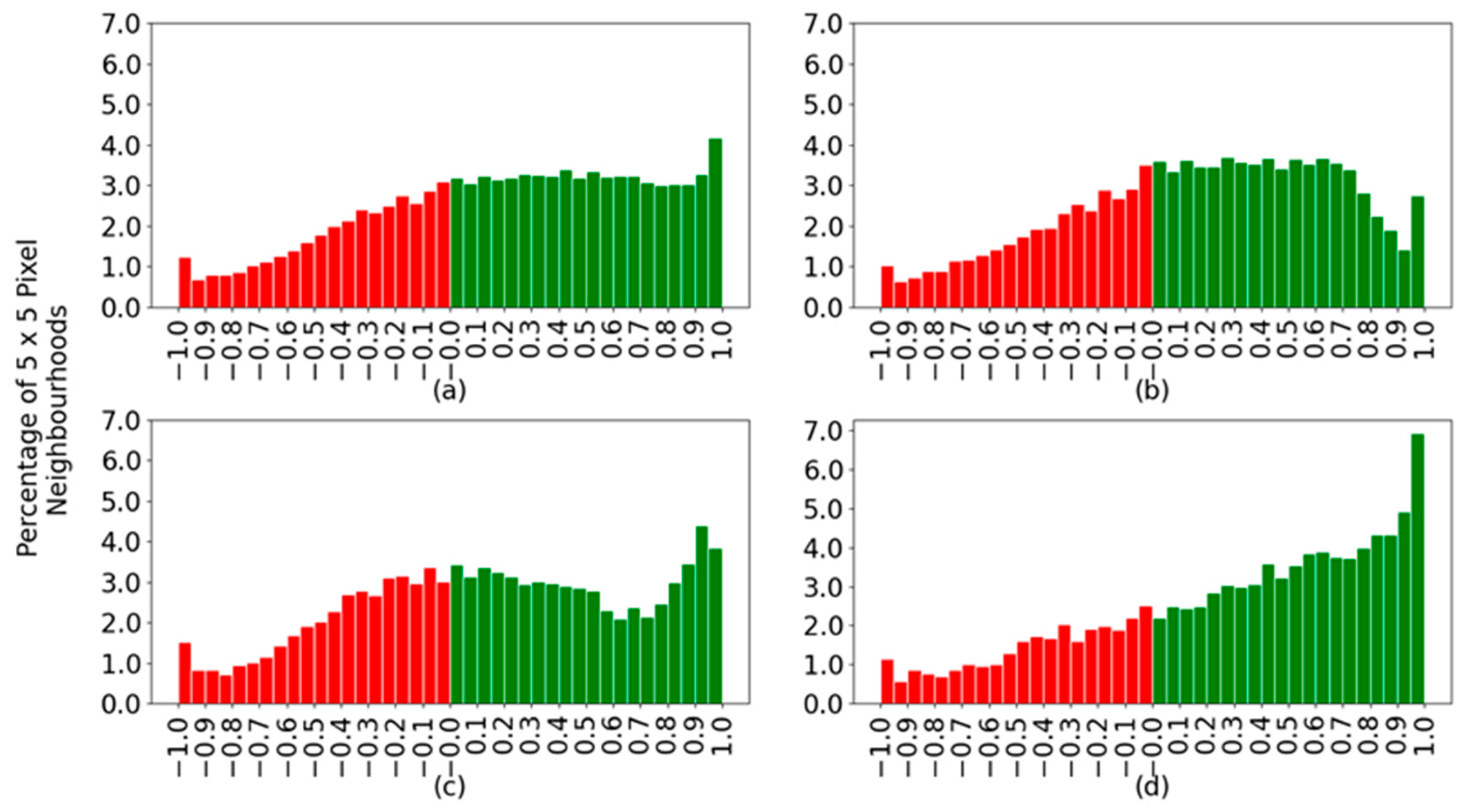Figure 9 shows histograms created by applying the described difference of probabilities to all spectra. Positive values indicate correctly classified spectra, shown in green, and negative values correspond to incorrectly classified spectra, shown in red. The histograms contain data from all spectra together and separated by species.

Figure 9a indicates that the correctly classified spectra in green spread across the range of possible confidence values between zero and one, with a slight peak at the highest confidence. One would like to have a single bar at the value of one. With the wrongly classified spectra, there is a decay toward the more wrongly confident values, those closer to minus one, which is good. The optimal case would be to have no red bars in the histograms. When considering each species separately, the sardines (Figure 9d) are more confidently classified and with a good slope on the green bars towards the highest confidence values. The main difference between horse and Atlantic mackerel is that although the former has an overall better classification percentage, 65.5% in Table 4 versus 58.9% for the latter, the Atlantic mackerel has more spectra at larger confidence values. For example, compare the size of the bar for a confidence value of 0.9 in Figure 9b,c.

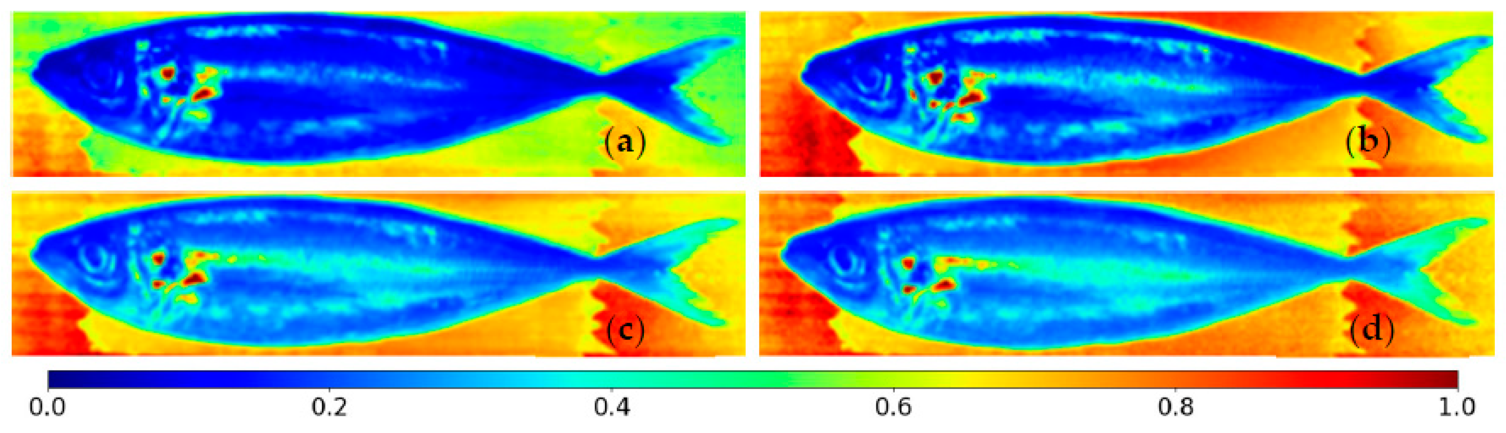
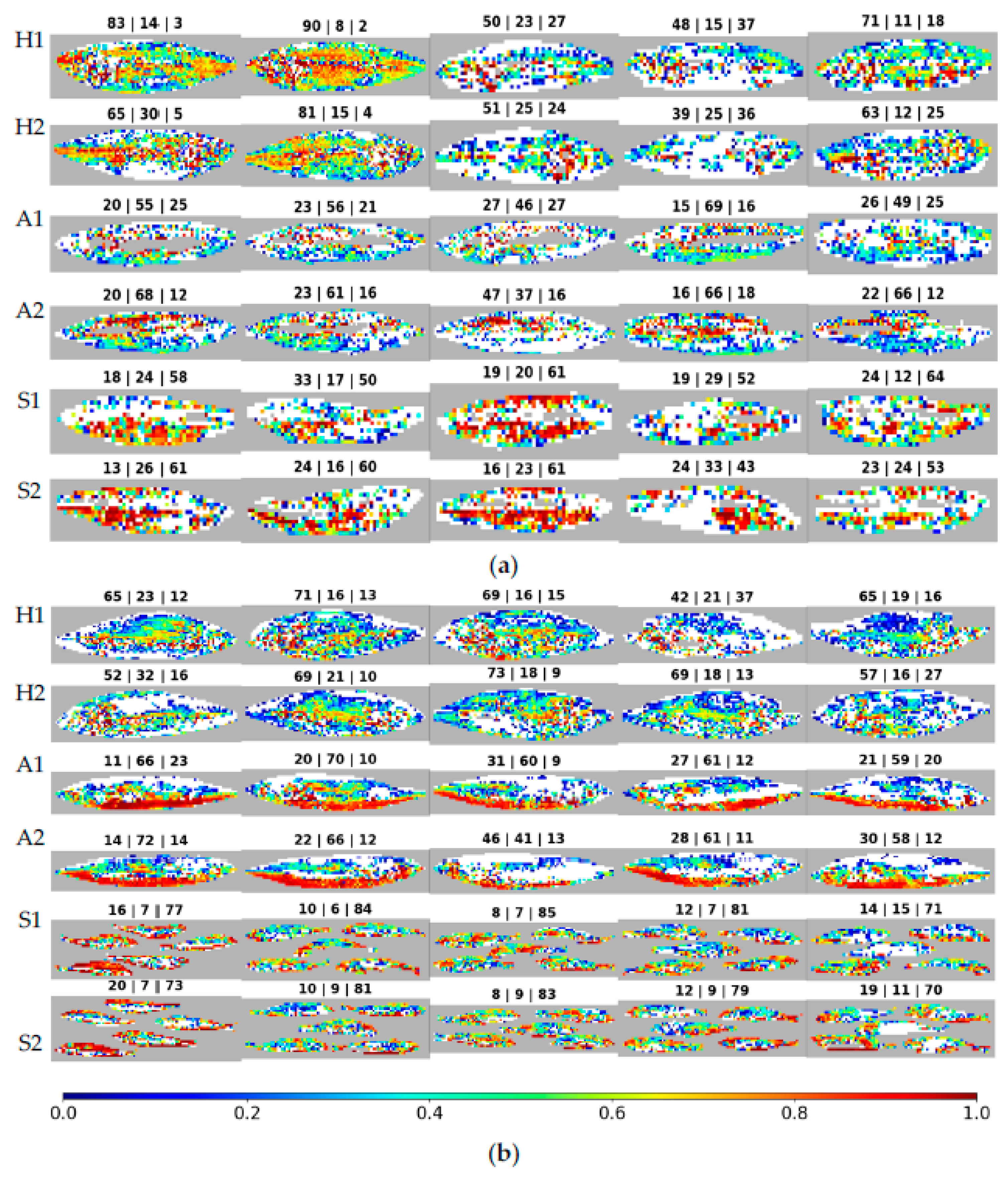
Figure 10 shows the same results as in Figure 9 but allows one to see the distribution of correct spectra at the fish position where they come from. Image construction has the following rules: spectra that were not classified, such as ruled-out background and saturated or noise-affected spectra, are shown in grey; incorrectly classified spectra that originated the red bars in Figure 9 are now displayed in white; and the correctly classified spectra are depicted through a color gradient based on the difference of probabilities. This difference is again between the probabilities of the correct and most probable incorrect classes. Above each image appears the percentage of spectra classified as being from each species, in the following sequence: horse mackerel, Atlantic mackerel, and sardines. The rows appear in pairs, corresponding to different sides of the same fish/fishes.

When analyzing the figure, the most striking characteristic is the tendency of various classification confidence values to show up all over the fish, visible by the colors mixing randomly. Next, the number of correctly classified spectra varies significantly, even between individuals of the same species. This characteristic is visible from the variation in the size of the white regions between various fish. It is also noticeable when analyzing the percentage of correct spectra, which is the opposite of the white spaces. The first batch’s (Figure 10a) second horse mackerel (counting from the left) shows 90% and 81% of spectra correctly classified for each imaged side, with 8% and 15% incorrectly classified as Atlantic mackerel, showing very good discernment. Meanwhile, the first batch’s fourth sardine has 52% and 43% of spectra correctly classified, with 29% and 33% incorrectly classified as Atlantic mackerel, showing less discernment while yet classifying most spectra as the correct species. Still, in the first batch, the third Atlantic mackerel presents even worse values, with 46% and 37% of correctly classified spectra on both fish sides. Side two of this fish would be wrongly classified when using a majority vote, as the most significant number of spectra, namely 47%, are attributed to horse mackerel. When looking for differences between the first and second batches of fish, the average of correctly classified spectra, as shown in

Table 5. Average of the percentage of correctly classified spectra per batch.

Fish Species	Correctly Classified Spectra (%)
	Batch 1	Batch 2
Horse mackerel	64.2	63.3
Atlantic mackerel	57.4	61.4
Sardine	56.4	78.5

for horse mackerel, is 64.2% for the former and 63.3% for the latter, which are close values. With Atlantic mackerel, these values change to 57.4% and 61.4%, indicating a slightly better outcome in the second batch. For sardines, the values are 56.4% and 78.8%, with a clear advantage for the second batch.

The horse mackerels in the first batch, displayed in the first pair of rows in Figure 10a, show differences from sample to sample, with some fish having 39% of spectra correctly classified and others having 90%. This variability is also present in the trust values, as a rainbow of colors fills the fish in Figure 10a. Within the fish with the highest percentage of correct classifications in the first batch, the second one, the trust strength seems to be higher in the middle section of the fish and reduces as one moves away from this section. However, in the second batch, seen in the first pair of rows in Figure 10b, the behavior is more uniform between samples. The percentage of correct classifications is between 42% and 73%, and the trust in these classifications is random but still shows slightly higher trust towards the middle section of the fish.

The Atlantic mackerels in the first batch, displayed in the second pair of rows in Figure 10a, show discarded spectra, color-coded in grey, concentrated in the middle portion of the fish. The correctly classified spectra offer varying levels of trust seen with brown/red and blue patches clustered together in different regions of the fish, revealing no identifiable pattern and varying between samples. In the second batch, seen in the second pair of rows in Figure 10b, a pattern emerges with the bottom half of the fish correctly classified with a high trust level, seen in brown/red. By contrast, the upper half of the fish shows a lower level of trust and more incorrect classifications, as seen in white. The percentages of correctly classified spectra vary between 37% and 69% in the first batch and between 41% and 72%, an identical variation between batches.

Lastly, sardines, displayed in Figure 10a,b, in the last pair of rows, behave uniformly within batches but vary significantly between these batches. While the first batch of sardines has between 43% and 64% correctly classified spectra, the second batch has 70% to 85%. While the trust values vary within each fish, the overall strength of sardine classifications is usually higher than for the other species, visible by the higher presence of yellow to red/brown color-graded regions in the figure. The only exception to this trend is the Atlantic mackerel in the second batch. In the first batch, sardines have the broadest areas, between species, of fish with the highest classification confidence. Nevertheless, they do not have the greatest percentages of correctly classified spectra.

On average, as seen in Table 5, Atlantic mackerel and sardines have the largest percentages of correctly classified spectra in the second batch. With horse mackerel, the first and second batches are only slightly different, with an advantage for the first.

3.6. Feature/Camera Selection

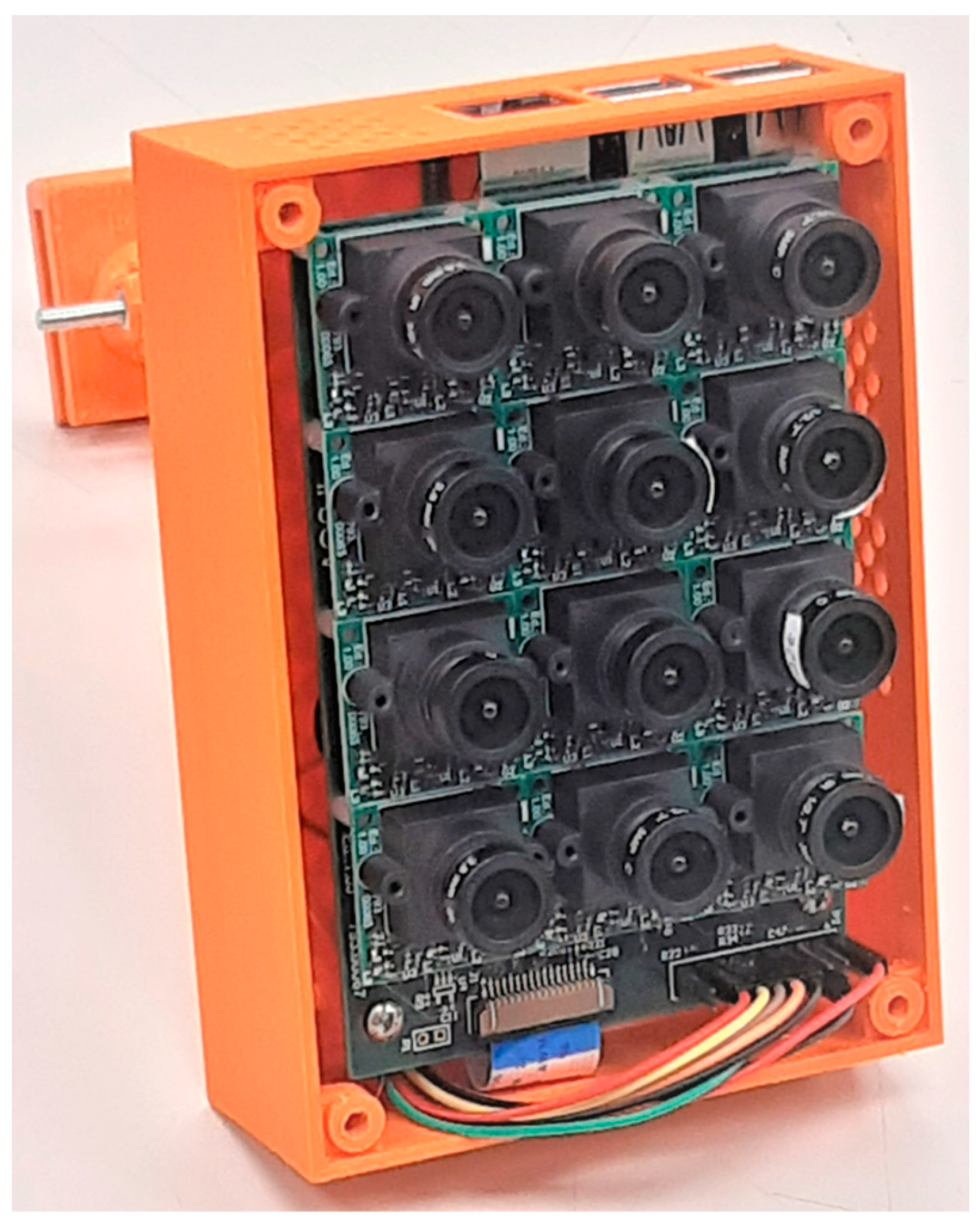
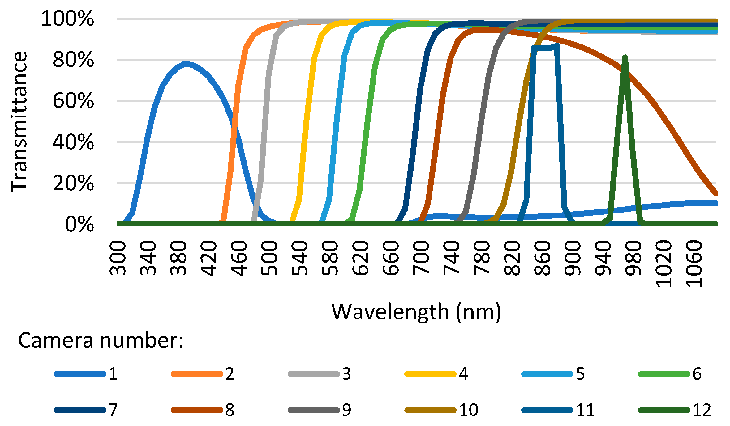
This section reports a study on the possibility of using less than twelve cameras to classify fish species. Tests were performed using one to twelve cameras. The results of this analysis are shown in

Table 6. Balanced accuracies for various classifiers and different numbers of input features/cameras.

Classifier	Balanced Accuracy (%)
	Number of Cameras
	12		11	10	9	8	7	6	5	4	3	2	1
KNN	56.7	Seq.	57.2	57.4	57.2	56.5	56.0	55.8	54.1	51.9	48.8	45.9	38.5
		Uni.	55.1	53.8	53.8	53.2	51.3	50.8	49.2	48.4	46.7	41.3	34.9
MP	64.4	Seq.	62.8	62.6	63.0	63.3	61.6	55.3	57.0	54.6	52.1	50.0	39.9
		Uni.	61.6	58.7	57.3	57.6	54.9	53.5	52.4	51.0	49.5	44.5	39.9
SVM	65.3	Seq.	65.2	65.3	64.9	63.5	61.4	58.9	57.4	54.5	50.5	48.3	38.5
		Uni.	-	60.2	58.5	-	-	53.0	50.4	50.1	48.2	42.8	-

. The values for the KNN and MP with twelve cameras are those from Table 3. For SVM, a slightly different gamma was used, but for twelve cameras, the result is the same as in Table 3. The univariate feature selection generally leads to worse outcomes than the sequential feature selection (SFS) for the three types of classifiers studied. That is why some results are not given for univariate selection, and the following analysis will focus solely on SFS.

KNN returns a balanced accuracy of 56.7% using all twelve cameras. With eleven, ten, and nine cameras, one obtains improvements of 0.5, 0.7, and 0.5 p.p., respectively. The best result is achieved with ten cameras, at 57.4%. This is good since it could allow reducing the MultiCam size and cost. With six cameras, which would mean a significant downsizing, the balanced accuracy drops 1.6 p.p to 55.8%. The MP returns a balanced accuracy of 64.4% using all features. Even though the results improve when going down from eleven to eight cameras, reaching 63.3%, after that, they drop below 62%, never surpassing the case with twelve cameras. With six cameras, the balanced accuracy is 55.3%. SVM with twelve cameras shows the best results using all features, with 65.3%. However, obtaining the same balanced accuracy is possible with ten cameras, even though it means discarding cameras number 3 and 6, whose cut wavelengths are 495 nm and 630 nm, respectively, and gathering, supposedly, less information. With SVM and six cameras, the balanced accuracy drop is 6.4 p.p.

3.7. Teflon vs. Spectralon Performance

This experiment employed a large white Teflon strip covering the entire area of the fish positions, allowing the reflectance calculation to use pixel-wise measurements. The second white target analyzed was Spectralon. It covers only a small area compared to the fish area. It is not in the same position as the fish, requiring the reflectance calculation for all pixels to use a single averaged value of Spectralon’s spectra. The third target is a small region of the Teflon strip with the same area as the Spectralon target and outside the fish position. This third target allows the comparisons to be more equitable. Nine classifiers, three for each of the three machine learning algorithms used, and one for each dataset of reflectances determined with the three different white targets were created. The hyperparameters used are those described in Section 3.2. The balanced accuracies obtained from these models are shown in

Table 7. Balanced accuracy per spectra for different white targets. The Teflon strip values are the same as in Table 3.

Classifier	Balanced Accuracy (%)
	Teflon Strip	Teflon Target	Spectralon Target
KNN	56.7	57.7	56.0
MP	64.4	63.7	62.5
SVM	65.3	65.1	63.6

. The results for the Teflon strip are those from Table 3. For the MP and the SVM, when changing from the Teflon strip to the Teflon target, there is a drop of 0.7 p.p. and 0.2 p.p., respectively, to 63.7% and 65.1%, which is expectable since the latter white has a smaller area than the former. Surprisingly, for the Teflon strip and the Spectralon target, although the latter is usually a more accurate reference, the drop is 1.9 and 1.7 percentage points, to 62.5% and 63.6%. The KNN classifier follows a different trend, with the Teflon target having the best result of 57.7%, but the Spectralon target again yields the worst result, 56.0%.

3.8. Estimation of the Number of Spectra of Each Species

The classification algorithms do not offer a 100% correct classification ability. Consequently, the direct classification results are not an immediate measure of the number of spectra available for each species in the captured images. In addition, the spectra of one species can be wrongly classified as belonging to another species. To resolve this issue, one can use the confusion matrix results to estimate the real number of spectra, considering the misclassification probabilities. With the confusion matrix given by:

True label	Horse mackerel	$P_{HH}$	$P_{HA}$	$P_{HS}$
	Atlantic mackerel	$P_{AH}$	$P_{AA}$	$P_{AS}$
	Sardine	$P_{SH}$	$P_{SC}$	$P_{SS}$
		Horse mackerel	Atlantic mackerel	Sardine
		Predicted label

P_XY represents the probability of a spectrum of species X being classified as being from species Y. As previously, H, A, and S stand for horse mackerel, Atlantic mackerel, and sardines, respectively. Knowing that Q_Hmea, Q_Amea, and Q_Smea are the quantities that the classification algorithm has returned for the species, one may write:

$$\left(\begin{array}{c}{Q}_{Hmea}\\ Q_{Amea}\\ Q_{Smea}\end{array}\right)=\left[\begin{array}{ccc}{P}_{HH}& P_{AH}& P_{SH}\\ P_{HA}& P_{AA}& P_{SA}\\ P_{HS}& P_{AS}& P_{SS}\end{array}\right]\left(\begin{array}{c}{Q}_{Horse}\\ Q_{Atlantic}\\ Q_{Sardine}\end{array}\right),$$

And therefore:

$$\left(\begin{array}{c}{Q}_{Horse}\\ Q_{Atlantic}\\ Q_{Sardine}\end{array}\right)={\left[\begin{array}{ccc}{P}_{HH}& P_{AH}& P_{SH}\\ P_{HA}& P_{AA}& P_{SA}\\ P_{HS}& P_{AS}& P_{SS}\end{array}\right]}^{-1} \left(\begin{array}{c}{Q}_{Hmea}\\ Q_{Amea}\\ Q_{Smea}\end{array}\right),$$

where Q_Horse, Q_Atlantic, and Q_Sardine represent the real quantities of spectra of horse mackerel, Atlantic mackerel, and sardines, respectively, to be estimated in the collected images. Note that the confusion matrix is transposed. The results obtained with this method are as accurate as the statistics in creating the confusion matrix.

4. Discussion

4.1. Final Tuned Model Classification Accuracy and Classification Trust

Comparing the algorithms, while the KNN performed the worst out of the three models, returning predictions with a balanced accuracy of 56.7%, it was not too far behind the other models, showing good results considering its simple methodology that required only one second of training time. The MP, trained for 3 min and 2 s, returned 64.4% balanced accuracy, while the SVM, trained for 8 h, 29 min, and 36 s, returned 65.3%. While the MP proved to be more computationally efficient, the SVM proved more accurate.

From the confusion matrices’ diagonals in Table 4, all algorithms show a skewed accuracy, correctly classifying the sardines’ spectra at a higher rate than those of the other classes. A possible cause immediately comes to mind is that sardines have scales different from horse mackerel, and Atlantic mackerel do not have scales. However, when looking at the first batch, the sardine spectra are not correctly classified at more significant percentages than the other species’ spectra. The large difference occurs only with the second batch of sardines where a significant difference existed, namely the size of the fish, with each fish being smaller and probably younger, which may mean better features for class separation. In addition, the number of spectra available deriving from 5 × 5 regions is 8540 in the second batch against 4075 in the first. In the present case, the larger number of spectra is not a reasonable explanation for the better results of the second batch since the horse mackerel class has a significantly greater number of spectra than the other classes and still does not have the largest percentage of correctly classified spectra (see Table 5). One possibility is that the variability in the second batch is described accurately by the 8540 spectra, leading to good results. Usually, in machine learning work, the results originate from a mix of the influence of the sample features and the amount of data available to train the classifiers; this case appears to be similar.

The best SVM created can correctly classify large portions of each fish, despite highly variable confidences (see Figure 10). It is hard to understand what might cause this variability, as one would expect to have nearby spectra with approximate confidence values. The variable confidences may indicate that each fish’s position differs significantly from the rest. Still, this thesis is contradicted by, in some cases, certain regions of the fish having similar confidence values. Therefore, it might be that the differences originate from numerical issues. The authors do not know at present, and more testing is necessary to understand this issue better.

The first batch’s horse mackerels showed significant differences from sample to sample, with some samples having 90% correct spectra classification and others having 39% (see Figure 10). Given that all the samples of one batch are obtained under the same setup without disturbances, it precludes lighting or hardware issues as the cause for the differences between samples of the same species. Therefore, the reason is more likely natural biological differences in the individual fish, presenting with enough different reflective properties to fall outside the learned pattern for its species.

The Atlantic mackerel in the second batch displayed one of the most consistent cases of a region presenting high-confidence classification values in our experiments. This consistency might have to do with this region corresponding to the “stripes” in the fish, but it cannot be the only reason since, for the same species in the first batch, this does not occur. Consequently, it might have something to do with the relationship between lighting, fish thickness, and “stripes”; if it were just the lighting, the effect would also be present in the horse mackerel of the second batch, and that is not the case.

4.2. Feature Selection Performance

Our results suggest a tendency for balanced accuracy to reduce with the number of cameras used. This reduction is expectable as the models receive less information. However, this is not always the case. For KNN, ten cameras outperform twelve, and SVM with ten cameras shows the same balanced accuracy as with twelve. This phenomenon probably occurs because the two discarded highpass filters do not add extra information to the whole group of filters, at least for the used dataset. Fewer features providing better results than more features is not an exclusive characteristic of the present application.

From the point of view of cost, it is interesting to have fewer cameras in the MultiCam; however, discarding two cameras from twelve is good but not a game changer. Nevertheless, it may save some physical space, two optical filters, and the camera chip and optics when building a MultiCam. Using twelve cameras might nonetheless be advisable as the extra information may be relevant when training with more samples. Still, the prospects for reducing the number of cameras in the current application are good.

4.3. Teflon vs. Spectralon Performance

In general, models employing reflectances calculated from Spectralon performed worse than those with reflectances determined with Teflon. When comparing the Spectralon target with the Teflon strip of lower diffuse reflectance, one sees that measuring the incident light in each fish pixel with Teflon is better than measuring it outside the fish pixels with Spectralon. One possible explanation for this phenomenon is the lack of lighting uniformity over the test table, which one may expect to exist in almost all real-life and low-cost setups required for widespread applications. More difficult to understand is why a Teflon target of the same area as the Spectralon and placed outside of the fish pixels’ positions leads to better results. A possible reason is again the non-uniformity in the lighting. Since the Teflon target is closer to the fish than the Spectralon, it may provide more realistic measurements of the fish’s lighting. Even though unexpected, these results are highly relevant to understanding that using high-cost white targets is not always necessary when making spectroscopy applications. A Teflon target can be good enough. Using a Spectralon target the size of the Teflon strip would be relevant from the scientific point of view but would be impractical for widespread application due to its cost.

4.4. Fish Imaging

The developed spectra identification method does not require fish to be separately measured, as has been the case in our test setup. However, capturing fish in an image containing, for example, seawater, fishing net, or boat regions would require further work in developing an image segmentation preprocessing step to separate the fish pixels/spectra from those belonging to other classes. Once the fish pixels/spectra are separated from the rest, they can be given to the classifier. For easier pixel separation, one can think of the fish passing under the camera via a conveyor belt of a color that allows easy separation between the fish and the background. The conveyor belt solution probably allows a more accurate estimation of fish quantities since there is no risk of fish overlap or loss of fish pixels due to incorrect segmentation from the background. Nevertheless, if the whole fish is visible, it may be more reasonable to consider the entire fish image for classification instead of small regions, even if the spectral information might help get better classification results. The authors still believe that having the ability to classify overlapping fish is relevant since, in fishing activities, the overlap is frequent.

4.5. Comparison with Previous Work

Two previous works, Benson et al. [9] and Ren et al. [10], are directly related to the present one in their use of machine learning and spectroscopy to identify fish species. Benson et al. reported accuracy rates of 91.5% for fish species identification, significantly better than those obtained in the present work. However, since their method is destructive due to the use of the fish otolith for classification, it is useless for accounting for fish quantities. Their measurement method is Fourier Transform Infrared (FTIR) spectroscopy, which is more complex and expensive than reflectance spectroscopy, as it usually involves an interferometer with moving parts and a laser for calibration. Ren et al. reported classification accuracies of 98.2%. Their samples were fish muscle homogenates, which makes their process also destructive. In the current work, the spectra are mainly from the fish skin. Homogenates may partly explain the good results because they help stabilize sample variability. When imaging the skin, without any preparation, one experiences its whole variability, with the extra trait of the skin’s high reflectivity that complicates diffuse reflectance measurements. In addition, Ren et al. used laser-induced breakdown (LIBS) and Raman spectroscopy, which are significantly more expensive than the reflectance spectroscopy used here, preventing widespread use. Building a low-cost Raman spectrometer is more complex than a reflectance spectrometer due to the smaller signal intensity involved in the former. Ren et al. used convolutional neural networks, which were not employed here since the MultiCam spectra dimensionality is small, namely twelve. Ren et al.’s data dimensionality was approximately 7000.

4.6. Practical Applications

The automatic calculation of the amount of fish captured per species will, hopefully, be part of equipment such as MONICAP [13] from the Portuguese company XSealence [14]. This equipment is installed onboard large fishing vessels and automatically sends information to a land center. From the center, reports may be forwarded automatically to the state authorities for monitoring fishing activities. This would allow these authorities to have a more accurate idea of the captured species at each moment and would simultaneously enable them to combat the fishing of unauthorized species and the fraudulent reporting of the amount of fish caught. Another possibility is to place a MultiCam camera at the entrances of fish markets to automatically control all the fish coming into the markets.

5. Conclusions

It is possible to separate fish from three species, namely, horse mackerel, Atlantic mackerel, and sardines, using a low-cost camera equipped with twelve filters, nine highpass and three bandpass, and an SVM. The identification uses small fish regions instead of whole fish. The choice of the highpass filters was due to their low cost. Their bands overlap; therefore, there is a relevant correlation between the information of the various filters. Nevertheless, the machine learning algorithms were able to use this information effectively. To the best of the authors’ knowledge, this work is unique in the scientific literature regarding fish reflectance spectra separation with machine learning while simultaneously keeping the fish whole. In fact, with the present work, more questions seem to be raised than answers given. Sardines have the best true classification percentage of 71.5%, while horse mackerel and Atlantic mackerel exhibit true detection percentages of 65.5% and 58.9% with the SVM. This results in a balanced accuracy of 65.3% with twelve cameras. Ten cameras provide the same accuracy value. These values are far from the 33% expected for a random classification. The present work also proposes a method to estimate the total amount of spectra available in gathered images for each species from the confusion matrix. Our results with a white target made of low-cost Teflon were better than with an expensive Spectralon target, possibly because the target extension and placement resulted in more accurate lighting measurements.

The less positive outcomes of the experiments are the high variability in classification confidence for contiguous regions and the significant differences in the percentage of correctly classified spectra between fishes. The cause of the former is unknown, and the latter seems to result from biological variability. The classification used 48,741 spectra of 5 × 5 pixel regions from 10 horse mackerel, 10 Atlantic mackerel, and 30 sardines. The number of fish is not larger because this is an exploratory study of a method not currently in use. These results should be confirmed with a greater number of fish imaged.

For future work, testing only bandpass filters to see if that helps improve the results would be relevant. Another possible approach is to calculate reflectances with a large Spectralon target to see the effect on the results. This test would be merely for scientific reasons because it is not affordable for widespread application. The present study opens up new possibilities and many questions requiring further work. Increasing the number of fish used in the analysis is a must.

References

1. Bjørndal, T.; Brasão, A.; Ramos, J.; Tusvik, A. Fish Processing in Portugal: An Industry in Expansion. Mar. Policy 2016, 72, 94–106. [Google Scholar] [CrossRef] [Green Version]
2. Bjørndal, T.; Lappo, A.; Ramos, J. An Economic Analysis of the Portuguese Fisheries Sector 1960–2011. Mar. Policy 2015, 51, 21–30. [Google Scholar] [CrossRef]
3. Jayasundara, D.; Ramanayake, L.; Senarath, N.; Herath, S.; Godaliyadda, R.; Ekanayake, P.; Herath, V.; Ariyawansha, S. Multispectral Imaging for Automated Fish Quality Grading. In Proceedings of the 2020 IEEE 15th International Conference on Industrial and Information Systems (ICIIS), Rupnagar, India, 26 November 2020; IEEE: Piscataway, NJ, USA, 2020; pp. 321–326. [Google Scholar]
4. Menesatti, P.; Costa, C.; Aguzzi, J. Quality Evaluation of Fish by Hyperspectral Imaging. In Hyperspectral Imaging for Food Quality Analysis and Control; Elsevier: Amsterdam, The Netherlands, 2010; pp. 273–294. ISBN 978-0-12-374753-2. [Google Scholar]
5. Cheng, J.-H.; Sun, D.-W. Hyperspectral Imaging as an Effective Tool for Quality Analysis and Control of Fish and Other Seafoods: Current Research and Potential Applications. Trends Food Sci. Technol. 2014, 37, 78–91. [Google Scholar] [CrossRef]
6. Kolmann, M.A.; Kalacska, M.; Lucanus, O.; Sousa, L.; Wainwright, D.; Arroyo-Mora, J.P.; Andrade, M.C. Hyperspectral Data as a Biodiversity Screening Tool Can Differentiate among Diverse Neotropical Fishes. Sci. Rep. 2021, 11, 16157. [Google Scholar] [CrossRef] [PubMed]
7. Fernandes, A.M.; Franco, C.; Mendes-Ferreira, A.; Mendes-Faia, A.; da Costa, P.L.; Melo-Pinto, P. Brix, PH and Anthocyanin Content Determination in Whole Port Wine Grape Berries by Hyperspectral Imaging and Neural Networks. Comput. Electron. Agric. 2015, 115, 88–96. [Google Scholar] [CrossRef]
8. Gewali, U.B.; Monteiro, S.T.; Saber, E. Machine Learning Based Hyperspectral Image Analysis: A Survey. arXiv 2018, arXiv:1802.08701. [Google Scholar] [CrossRef]
9. Benson, I.M.; Barnett, B.K.; Helser, T.E. Classification of Fish Species from Different Ecosystems Using the near Infrared Diffuse Reflectance Spectra of Otoliths. J. Infrared Spectrosc. 2020, 28, 224–235. [Google Scholar] [CrossRef]
10. Ren, L.; Tian, Y.; Yang, X.; Wang, Q.; Wang, L.; Geng, X.; Wang, K.; Du, Z.; Li, Y.; Lin, H. Rapid Identification of Fish Species by Laser-Induced Breakdown Spectroscopy and Raman Spectroscopy Coupled with Machine Learning Methods. Food Chem. 2023, 400, 134043. [Google Scholar] [CrossRef] [PubMed]
11. Cardoso, C.; Lourenço, H.; Costa, S.; Gonçalves, S.; Nunes, M.L. Survey into the Seafood Consumption Preferences and Patterns in the Portuguese Population. Gender and Regional Variability. Appetite 2013, 64, 20–31. [Google Scholar] [CrossRef] [PubMed]
12. Almeida, C.; Karadzic, V.; Vaz, S. The Seafood Market in Portugal: Driving Forces and Consequences. Mar. Policy 2015, 61, 87–94. [Google Scholar] [CrossRef] [Green Version]
13. MONICAP. Available online: https://www.xsealence.pt/en/equipamentos/monicap/ (accessed on 28 July 2023).
14. XSealence. Available online: https://www.xsealence.pt/ (accessed on 28 July 2023).
Figure 1. The MultiCam is a multispectral camera.
Remotesensing 15 03952 g001
Figure 2. The transmittance of filters for each MultiCam camera versus wavelength.
Remotesensing 15 03952 g002
Figure 3. Experimental setup.
Remotesensing 15 03952 g003
Figure 4. Examples of images from camera number one: (a) horse mackerel; (b) Atlantic mackerel; (c) sardine; (d) sardine. Cases (ac) are from the 2nd batch, while (d) is from the 1st.
Remotesensing 15 03952 g004
Figure 5. Pixel-wise reflectances for horse mackerel with cameras number (a) 1, (b) 2, (c) 10, and (d) 12. Reflectances smaller than zero and larger than one are set to zero and one, respectively.
Remotesensing 15 03952 g005
Figure 6. Objects for reference of the total intensity of light, WI: Te0—Teflon strip; Sp—Spectralon target; Te1—Teflon target.
Remotesensing 15 03952 g006
Figure 7. Reflectance spectra for fifteen samples.
Remotesensing 15 03952 g007
Figure 8. Average reflectance spectrum by species plus and minus one standard deviation.
Remotesensing 15 03952 g008
Figure 9. Histogram for the difference in SVM prediction probabilities: (a) all species; (b) horse mackerel; (c) Atlantic mackerel; and (d) sardine. Green and red bars correspond to correctly and incorrectly classified spectra.
Remotesensing 15 03952 g009
Figure 10. Difference in SVM prediction probabilities: (a) first batch; (b) second batch. For each batch, the first two rows are horse mackerel (H), the next two are Atlantic mackerel (A), and the last two are sardines (S). Above each image is the percentage of spectra classified as horse mackerel (H), Atlantic mackerel (A), and sardines (S), in this sequence. The fish side is the number, one or two, in front of the species letter (H, A, S).
Remotesensing 15 03952 g010