Article

Abandoned Land Mapping Based on Spatiotemporal Features from PolSAR Data via Deep Learning Methods

1
School of Geography and Remote Sensing, Guangzhou University, Guangzhou 510006, China
2
Key Laboratory of Natural Resources Monitoring in Tropical and Subtropical Area of South China, Ministry of Natural Resources, Guangzhou 510670, China
3
College of Hydrology and Water Resources, Hohai University, Nanjing 210098, China
4
Agricultural Science and Technology Information Research Institute, Guangxi Academy of Agricultural Sciences, Nanning 530007, China
5
School of Science, Chang’an University, Xi’an 710064, China
6
Aerospace Information Research Institute, Chinese Academy of Sciences, Beijing 100094, China
7
University of Chinese Academy of Sciences, Beijing 100049, China
*
Author to whom correspondence should be addressed.
Remote Sens. 2023, 15(16), 3942; https://doi.org/10.3390/rs15163942
Submission received: 16 June 2023 / Revised: 27 July 2023 / Accepted: 5 August 2023 / Published: 9 August 2023
(This article belongs to the Section Remote Sensing in Agriculture and Vegetation)

Abstract

:
Monitoring agricultural abandonment is essential in understanding the effects on the environment and food security. Polarimetric synthetic aperture radar (PolSAR) is an efficient approach for the monitoring of large-scale agricultural land cover in cloudy and rainy areas. However, previous studies have not taken advantage of the valuable phase information and not fully utilized the spatiotemporal features of farmland parcels, which has seriously limited the abandoned land identification accuracy. In this study, we developed a new method for the mapping of abandoned land based on the spatiotemporal features from PolSAR Single Look Complex (SLC) images via deep learning methods. First, backscattering coefficients (σ0VV, σ0VH) were derived, and the polarimetric parameters (entropy, anisotropy and mean alpha angle) were obtained based on Cloude–Pottier polarimetric decomposition. Then, the VGG16 deep convolutional network was innovatively used to extract spatial features from both the backscattering coefficients and polarimetric parameters. Next, the separability index was calculated to select the most effective spatial features. Finally, LSTM classifications were conducted based on the time series of backscattering features, the polarimetric parameters, the extracted spatial features and their combinations. The results showed that the introduction of multitemporal polarimetric parameters and spatial features both led to an improvement in the abandoned land identification accuracy. The combination of backscattering features, polarimetric parameters and spatial features yielded the best performance in identifying abandoned land, with producer’s accuracy of 88.29% and user’s accuracy of 84.03%. This study demonstrated the potential of polarimetric parameters and validated the effectiveness of spatiotemporal features in abandoned land identification. It provided a practical method for the production of a highly reliable abandoned land mapping in cloudy and rainy areas.

1. Introduction

Over the past several decades, agricultural land abandonment has become increasingly widespread due to rapid urbanization and rural depopulation. As a result, unmanaged agricultural lands are gradually being replaced by natural grass–herb formations and successive shrubs [1]. This can lead to food insecurity and various environmental effects, such as ecological restoration, soil erosion and changes in biodiversity [2,3,4,5,6]. Therefore, it is critical to monitor agricultural abandonment to understand regional food production and the related environmental outcomes. Agricultural abandoned lands are commonly fragmented and scattered, small in size and mostly distributed in mountainous areas, which presents significant challenges for their monitoring in a short time, as ground-based surveys are laborious and time-consuming [7]. Remote sensing techniques offer a more efficient approach to the monitoring of agricultural land abandonment quickly and on a large scale [8].
Many methods have been proposed to identify agricultural abandoned land via inverting remotely sensed radiance information at different spectral bands. These methods can be generally categorized into machine learning classification methods and land use/cover change detection methods [9]. Machine learning classification methods commonly extract spectral and phenological features from remote sensing data and use them to train a supervised classifier, such as random forest or support vector machine [10]. Compared to actively cultivated land, which is regularly sown, irrigated, tilled or harvested, unmanaged land is gradually covered by natural vegetation and presents different phenological characteristics. Alcantara et al. made use of the phenology metrics extracted from the time series data of MODIS imagery to identify abandoned land [11]. Likewise, Estel et al. captured the differences in the shape characteristics of the normalized difference vegetation index (NDVI) time series between cultivated land and abandoned land [12]. Land use/cover change detection methods conduct land use/cover classifications in multiple years and track the changes from cropland into other land cover types, such as natural grassland, shrubland or forests [13,14,15,16]. For example, Campbell, et al. combined a statistical land use database and MODIS data to analyze land use transition and acquired a global abandoned land map [17]. Zhang et al. used long-time-series 30 m Landsat land use products to identify the land use change trajectories and mapped the spatiotemporal distribution of abandonment in China [18]. Yin et al. estimated the possibility of agricultural land being used based on spatial–temporal metrics and detected abandonment from the possibility time series data [19]. Land use/cover change detection methods are less efficient because they depend on long-term remote sensing observations.
In many studies on agricultural abandonment detection, optical data from sensors such as MODIS, Landsat and SPOT are the primary data sources [1,10,12,14,15,20,21,22]. However, due to the influence of cloud contamination, optical data inevitably contain temporal gaps, which bring uncertainties in monitoring abandonment. In contrast, synthetic aperture radar (SAR) data have the capability of penetrating cloud and haze and thus offer an attractive option in land cover detection in cloudy and rainy regions [23]. Moreover, SAR data can provide complementary information to optical data, including the surface roughness, shape and moisture content of the observed ground [24,25]. Therefore, SAR is used independently or integrated with optical data to identify abandoned land [7,26,27]. For example, Stefanski et al. derived land use/cover change trajectories based on Landsat and ERS SAR data using a random forest classification method and acquired the distribution of abandoned land in Western Ukraine [25]. Yusoff et al. identified abandoned lands of paddy, rubber and oil palm using rule-based approaches based on ALOS-1 and 2 PALSAR multi-temporal data [28].
However, previous studies that have applied SAR data are commonly limited to the backscattering intensity information from the ground range detected (GRD) product, while the phase component of microwave radiation is rarely utilized. Polarimetric SAR (PolSAR) data can provide richer information containing both the intensity and phase information of electromagnetic waves. Parameters derived from polarimetric decomposition have shown capabilities of identifying crop types [29,30] and monitoring crop growth [31] and therefore are expected to have high potential in abandoned land identification. Additionally, most of the studies concerned with the temporal features derived from multitemporal observations ignore the valuable information about spatial features. It should be mentioned that, compared to non-abandoned cropland, which has a smoother texture and higher spatial homogeneity due to cultivation activities, abandoned land generally presents more irregular spatial texture features and higher heterogeneity [19]. Therefore, the combination of spatial and temporal features might have a greater contribution in enhancing the identification accuracy.
The most widely used methods to extract spatial features include the gray level co-occurrence matrix, wavelet transformation and spatial correlation calculation [32]. These spatial feature analysis methods show the weaknesses of low efficiency and high computational complexity. In recent years, with the rapid development of deep learning techniques, deep convolutional networks have shown strong performance in extracting and learning multi-scale spatial features and have been increasingly used in remote sensing applications such as land cover classification and change detection [33,34,35]. To better utilize spatiotemporal features, hybrid deep learning frameworks, such as the ConvLSTM network and FCN-LSTM network, have been developed in the remote sensing classification field [32]. Compared to the traditional machine learning algorithms, which manually define features and conduct classification, deep learning frameworks can automatically learn spatiotemporal features.
Based on the above insights, this study aims to (1) develop a practical method for the identification of abandoned land using spatiotemporal features from PolSAR data via a deep learning approach; (2) evaluate and compare the performance of different types of features, including backscattering coefficients, polarimetric parameters and convolution-based spatial features, in identifying abandoned land; and (3) apply the proposed method to map abandoned land in a study area.

2. Materials

2.1. Study Area

Jiexi County is selected as the study area. Located in eastern Guangdong Province in China, Jiexi County is characterized by rugged terrain, a variable climate and complex land use patterns, and it offers a representative example associated with monitoring agricultural land abandonment in rapidly urbanizing regions of China (Figure 1). Jiexi County covers an area of 1347 km2, most of which is covered by hilly and mountainous areas. Jiexi County has a south subtropical monsoon climate, which is characterized as warm and rainy. The annual total rainfall reaches 2084.8 mm, the annual average temperature is approximately 22.6 °C, and the total sunshine hours throughout the year reach 1837 h. The warm and favorable climate allows for the cultivation of up to three crops per year in a single field. This agricultural practice leads to a high degree of diversity in crop planting patterns throughout the county, with farmers adjusting their planting schedules and crop types to maximize yields. The dominant crop types include paddy rice, maize, peanut and various vegetables. The spatial distribution of cropland is fragmented and scattered due to the complex terrain conditions. The majority of croplands in Jiexi County are located in the southeastern region, where the terrain is mostly flat, and there are some croplands scattered in the mountain valleys of the northern and western regions.

2.2. Satellite Imagery

The Sentinel-1 satellites are equipped with dual-polarization channels (VV and VH) operating in the C-band frequency range and offer four different acquisition modes, including stripmap, interferometric wide swath, extra-wide swath and wave modes. The Sentinel-1 satellites provide a revisiting period of 12 days. In this study, Sentinel-1 Level-1 Single Look Complex (SLC) products operated with IW mode were applied. These SLC products have a swath of 250 km and a spatial resolution of 5 m × 20 m in the azimuth and range directions, respectively. In total, 30 tiles of Sentinel-1 data were downloaded from the Copernicus Open Access Hub (https://www.copernicus.eu/en, accessed on 16 June 2023), covering the acquisition period from 9 January 2021 to 23 December 2021 (Table 1).
To study the phenological features of different land cover types, the time series dataset of Sentinel-2 Level-2 products was acquired from the Google Earth Engine (GEE) platform. The time series data were preprocessed and downloaded from GEE, with preprocessing procedures including masking cloudy pixels, image mosaicking and time series reconstruction using a linear interpolation method.

2.3. Sample Data Collection

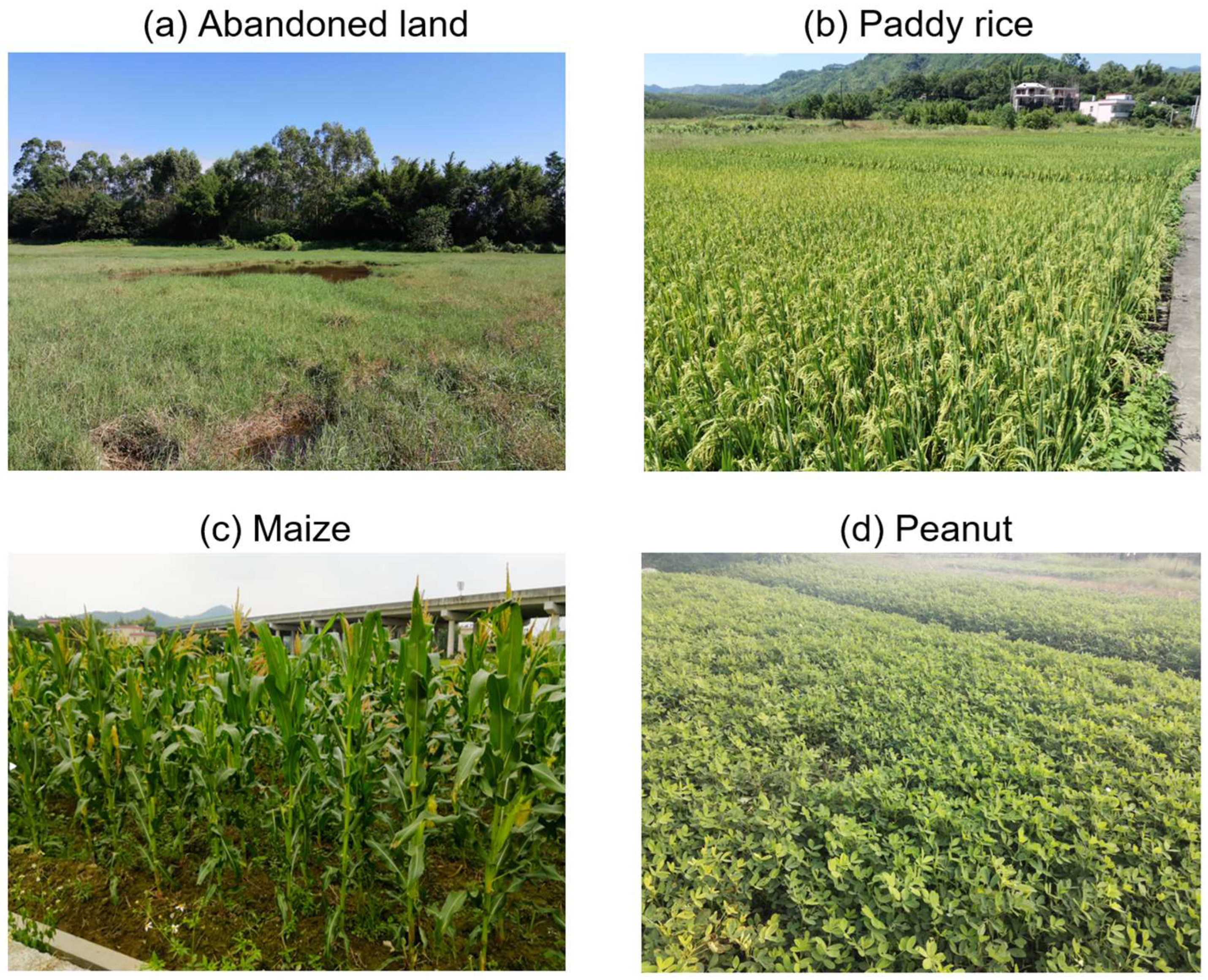
The sample data were collected from a ground-based survey and visual interpretation. In May 2021, a field survey was conducted in the study area to collect samples of abandoned lands and non-abandoned lands, focusing on the dominant crop types, including paddy rice, maize and peanut (Figure 2). During the ground-based survey, 793 samples of abandoned land, 1026 samples of paddy rice, 75 samples of maize and 27 samples of peanut were collected. Figure 3 shows high-resolution Google Earth images of typical abandoned lands and non-abandoned lands. It is indicated that non-abandoned lands exhibit more regular texture features and higher intra-parcel homogeneity due to consistent farming activities. In contrast, abandoned lands exhibit more irregular textures and unclear boundaries due to the growth of natural vegetation. In order to supplement the sample dataset, based on their visual characteristics, additional samples were manually added to the dataset. As a result, a large sample dataset containing 6353 samples was constructed, including 2431 abandoned land samples, 2071 double rice samples and 1851 samples of other crop types. Due to the difficulty in distinguishing the features of maize and peanut in the images, they were not classified separately but were grouped together under the category of other crops. To prepare the dataset for modeling, the samples were randomly divided into training samples and validation samples at a ratio of approximately 7 to 3.

2.4. Farmland Parcel Data

Farmland parcel data were acquired from our previous work through the combination of image segmentation and manual revision based on the high-resolution Google Earth images. The image segmentation was performed using the D-LinkNet deep convolutional network. For areas where the segmentation results were suboptimal, the boundaries of the extracted parcel objects were manually revised to produce the farmland parcel map. Overall, a total of 107,381 farmland parcel objects was acquired in Jiexi County. The farmland parcel data were used to perform parcel-level abandoned land mapping in the last step of this work.

3. Methods

In this work, the abandoned land identification was implemented by the following steps (Figure 4): (1) Sentinel-1 SLC data were preprocessed to generate backscattering coefficients (σ0VV, σ0VH) and three polarimetric parameters (entropy (H), anisotropy (A) and mean alpha angle ( α ¯ )); (2) the VGG16 deep convolutional network was used to generate spatial features based on both the backscattering coefficients and polarimetric parameters of the Sentinel-1 SLC data; (3) the separability index was calculated for the selection of effective spatial features to distinguish abandoned land from other types; and (4) the Long Short-Term Memory (LSTM) network was applied to identify abandoned land based on the time series of multiple features, including backscattering features, polarimetric parameters and the VGG16-based spatial features.

3.1. Sentinel-1 SLC Data Preprocessing

The Sentinel-1 SLC products were preprocessed to extract backscattering coefficients and polarimetric parameters using the Sentinel-1 Toolbox in the ESA SNAP software (http://step.esa.int/main/toolboxes/sentinel-1-toolbox/, accessed on 16 June 2023).

3.1.1. Backscattering Coefficients

The SLC products were first subjected to orbit correction using the precise orbit files. Then, the images were radiometrically calibrated to transform the pixel digital values into the backscattering coefficients (σ0VV, σ0VH). The TOPSAR deburst operator was used to concatenate the separate successive bursts of each sub-swath to form one image. The images were subjected to the multi-looking operator with a window size of 4 × 1 in the range and azimuth directions, respectively. The refined Lee filter with a window size of 7 × 7 pixels was applied to mitigate speckle noise. The images were geocoded by the Range Doppler Terrain Correction tool to correct geometric distortions using the Shuttle Radar Topography Mission (SRTM) DEM data. Finally, the sigma values of all images were converted into decibel scale.

3.1.2. Polarimetric Parameters

The SLC data were radiometrically corrected and saved as complex-valued images to reserve phase components. Then, the deburst operation was performed to merge separate bursts into a single image. Subsequently, a 2 × 2 covariance matrix (C2) was generated at the pixel level using the polarimetric matrix generation operator. The multi-looking and speckle filtering processes were conducted.
Based on the representative eigenvalue–eigenvector-based Cloude–Pottier decomposition method, three polarimetric parameters, including the polarimetric scattering entropy H, the mean alpha angle α ¯ and the polarimetric anisotropy A, were derived [36]. Through the process of eigen-decomposition, the observed covariance matrix was expressed as follows (Equations (1) and (2)).
C 2 = U λ 1 0 0 λ 2 U T *
U = U 11 U 12 U 21 U 22 = u 1 u 2
where [U] is the orthogonal unitary matrix. u 1 and u 2 are the eigenvectors. λ1 and λ2 are the two eigenvalues of the coherency matrix and quantify the relative importance of each scattering mechanism to the total measured signal.
Based on the acquired eigenvalues and eigenvectors, the polarimetric scattering entropy H, mean alpha angle α ¯ and anisotropy A were calculated as follows (Equations (3)–(6)).
H = i = 1 2 p i log 2 p i
A = λ 1 λ 2 λ 1 + λ 2
α ¯ = i = 1 2 p i α i = p 1 α 1 + p 2 α 2
p i = λ i i = 1 2 λ i , i = 1 , 2
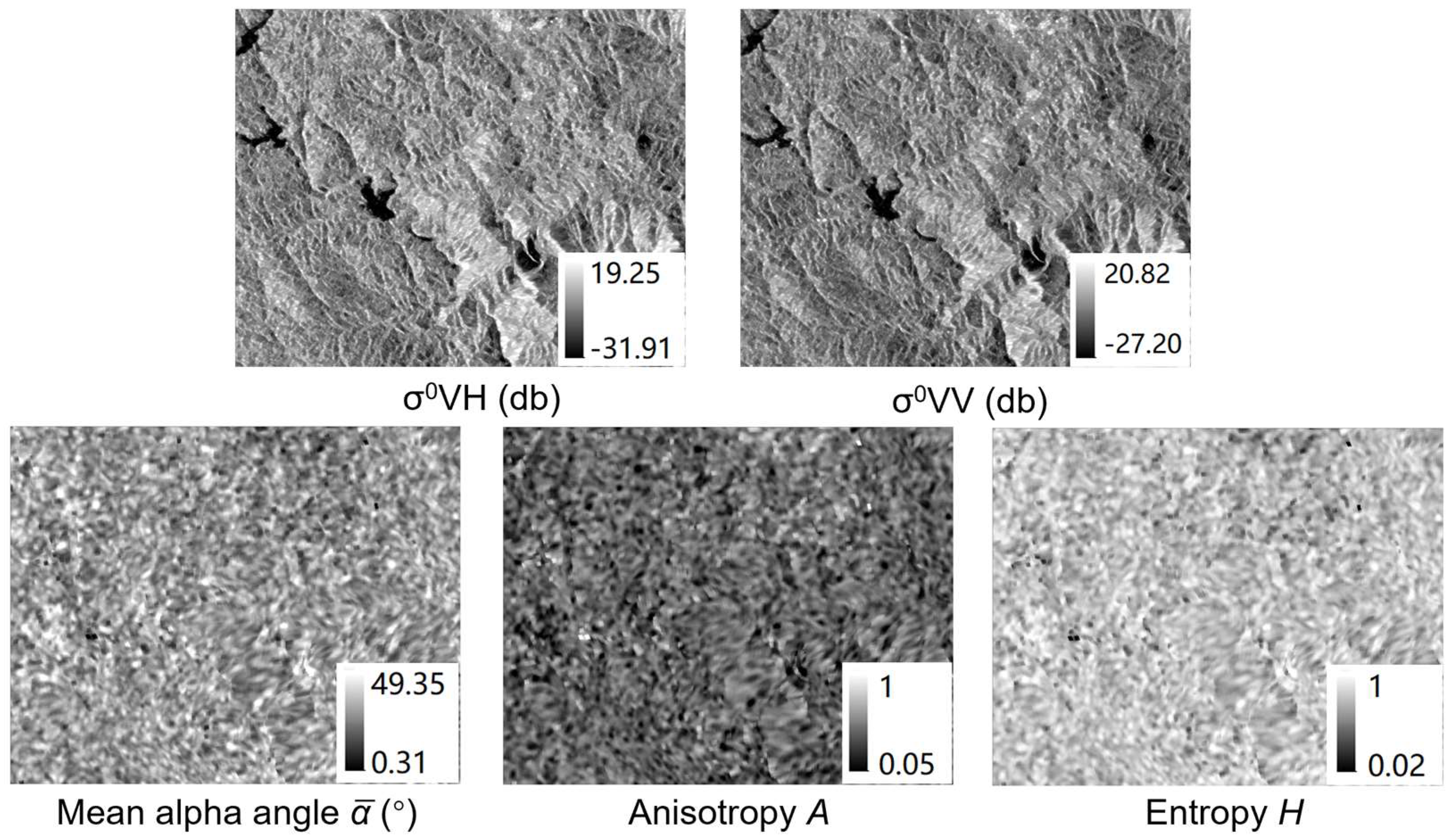
The polarimetric scattering entropy H measures the randomness of the scatterer. A larger H indicates higher scattering randomness. It ranges from 0 to 1, representing specifically identifiable scattering to completely random scattering. Anisotropy A describes the ratio between the first and second eigenvalues from the polarimetric decomposition. It measures the relative importance between the secondary scattering mechanisms. Angle α ¯ represents the scattering mechanism type in the scattering medium. It ranges from 0° to 90°, representing surface scattering to double-bounce scattering. Mean alpha angle α ¯ identifies the main scattering mechanism and represents the structure of the detected targets. The images of these three parameters are shown in Figure 5. Time series of H, A and α ¯ were used to describe the temporal variations in the scattering randomness and the scattering mechanism during the process of vegetation growth.

3.2. Spatial Feature Generation by VGG16 Network

The visual geometry group model (VGG) is a popular convolutional neural network proposed by Simonyan and Zisserman [37]. The VGG network presents superior performance, with classification accuracy of 92.7% in the ImageNet dataset, which contains over 14 million images belonging to 1000 classes. The VGG network has been applied to remote sensing image classification applications with satisfactory performance [38,39]. VGG16, a widely used VGG network, consists of 13 convolutional layers and 3 fully connected layers. In each convolutional layer, the image is convoluted with a 3 × 3 kernel size. Some of the convolutional layers are followed by a max-pooling layer with a 2 × 2 filter size. The max-pooling layer takes the largest value inside the filtering window and produces a new feature map. Therefore, to retain the original spatial features, ‘block1_conv2’ and ‘block2_conv2’ feature layers before the max-pooling operation were adopted in this work. It was demonstrated that deeper convolutional layers derived from the ten-meter-resolution data presented limited performance in land cover discrimination in a previous study [32]. Therefore, only the two shallow layers, ‘block1_conv2’ and ‘block2_conv2’, were selected. The VGG16 network was built using the Keras framework on top of Tensorflow.
In this work, VGG16-based spatial features were generated separately for the backscattering coefficients and polarimetric decomposition metrics, which were obtained from the Sentinel-1 SLC products. To composite the input image for the VGG16 network, the σ0VV, σ0VH and σ0VH/σ0VV were normalized to 0 to 1 using the maximum and minimum values of the band and then multiplied by 255, and they were then combined into a three-band image (Figure 6d). Similarly, the H, A, α ¯ feature bands were combined (Figure 6i). As the input data of the network required an image with dimensions of 224 × 224 × 3, the entire image covering the whole study area was divided into 570 tiles, each sized 224 × 224 pixels. These split tiles were input into the VGG16 network, and ‘block1_conv2’ feature layers with a size of 224 × 224 pixels and 64 channels and ‘block2_conv2’ feature layers with a size of 112 × 112 pixels and 128 channels were generated (Figure 6e,j). The ‘block2_conv2’ layers were then resized to the size of 224 × 224 pixels using the bilinear interpolation method. Consequently, a total of 192 spatial features were generated for each composite image, and the spatial features extracted from multiple observation phases constructed the high-dimensional time series.

3.3. Effective Spatial Feature Selection by Separability Index

To identify the most effective features from the high-dimensional VGG16-based spatial features, the separability index (SI) was calculated between each pair of classes for each spatial feature. SI, calculated using the mean values of a feature and the standard deviations of the feature (Equation (7)) [40], can evaluate the performance of a feature in discriminating different land cover types [41].
S I i j ( m , t ) = Δ i n t e r ( i , j ) Δ i n t r a ( i , j ) = μ i ¯ μ j ¯ 1.96 × ( σ i + σ j )
where the symbols i and j represent different land cover classes, m denotes the m-th feature being analyzed, and t refers to the t-th observation in the time series under consideration. μ i ¯ and μ j ¯ represent the mean values of a certain feature for class i and j, respectively. σ i and σ j refer to the standard deviations of this feature for class i and class j, respectively. The absolute difference between the mean values of two classes ( μ i ¯ μ j ¯ ) can be used to quantify the inter-class variability between these classes. On the other hand, the sum of the standard deviation values for each class ( σ i + σ j ) represents the intra-class variability. A higher SI value indicates better separability between two classes, which means that the feature is more effective in distinguishing between these two classes. The resulting SI values were then averaged to provide an overall measure ( S I ¯ ( m , t ) ) of the separability between abandoned land and the remaining classes. The average SI value ( S I ¯ ( m , t ) ) indicated how effectively the m-th feature could distinguish abandoned land from other classes on the t-th observation. By summing up the S I ¯ ( m , t ) values for each feature across all observations in the time series, a new variable S I s u m ( m ) was obtained (Equation (8)), which indicated the overall capability of the m-th feature to distinguish abandoned land from other classes, taking into account all observations in the time series.
S I s u m ( m ) = t = 1 T S I ¯ ( m , t )
where m refers to the m-th feature being analyzed, and t represents the t-th observation in the time series. T is the length of the time series observations.

3.4. LSTM-Based Abandoned Land Identification

LSTM is a specialized type of Recurrent Neural Network (RNN) that can avoid the vanishing gradient problem and learn long-term dependencies [42,43,44]. Thanks to its ability to capture long-term dependencies and relationships between past and present inputs, LSTM is well-suited for the analysis of sequential data. An LSTM cell is composed of three gates, including a forget gate (ft), input gate (it) and output gate (ot), that are used to regulate the flow of information within the cell. These gates in an LSTM cell are implemented through point multiplication operations that determine how much information can be retained or passed through. The forget gate in an LSTM cell uses a sigmoid function (Equation (9)) to decide which information should be discarded. This gate reads the previous output ht−1 and the new input xt and generates an output value between 0 and 1. A value of 0 means that the information is entirely forgotten, while a value of 1 means that the information is fully retained. By selectively forgetting irrelevant or outdated information, the LSTM network can better focus on the most important features of the sequential data.
f t = σ ( W f [ h t 1 , x t ] + b f )
where Wf is the weight matrix, bf is the bias item and σ is the sigmoid function.
Then, the LSTM cell determines which values to update and generates a new candidate vector using two additional layers: a sigmoid layer and a tanh layer. The sigmoid layer is used to decide which values to update in the cell status using Equation (10), while the tanh layer creates a new candidate vector using Equation (11). The sigmoid and tanh layers are then combined to update the status of the cell.
i t = σ ( W i [ h t 1 , x t ] + b i )
C ˜ t = t a n h ( W C [ h t 1 , x t ] + b C )
where Wi and Wc are the weight matrices of the input gate and input candidate element, respectively, and bi and bc are the corresponding biases.
After this, the state of the cell is updated from previous state Ct−1 to a new state Ct using Equation (12). The old state Ct−1 is first multiplied by the forget gate value ft, and the candidate value C ˜ t is multiplied by it. These two values are added together to form the updated cell state Ct.
C t = C t 1 × f t + C ˜ t × i t
In the last step, the LSTM cell generates its final output value ht. This is determined by the output gate ot and the current cell state Ct. The output gate ot decides which parts of the cell state to output by applying a sigmoid function (Equation (13)). The output value ht is calculated by multiplying the output gate ot by the updated cell state Ct in the form of a tanh function (Equation (14)). The final output value (ht) of the LSTM cell is determined by the output gate and the cell state (Equation (13) and (14)).
o t = σ ( W o [ h t 1 , x t ] + b o )
h t = o t × t a n h ( C t )
where Wo and bo are the weight matrix and bias, respectively.
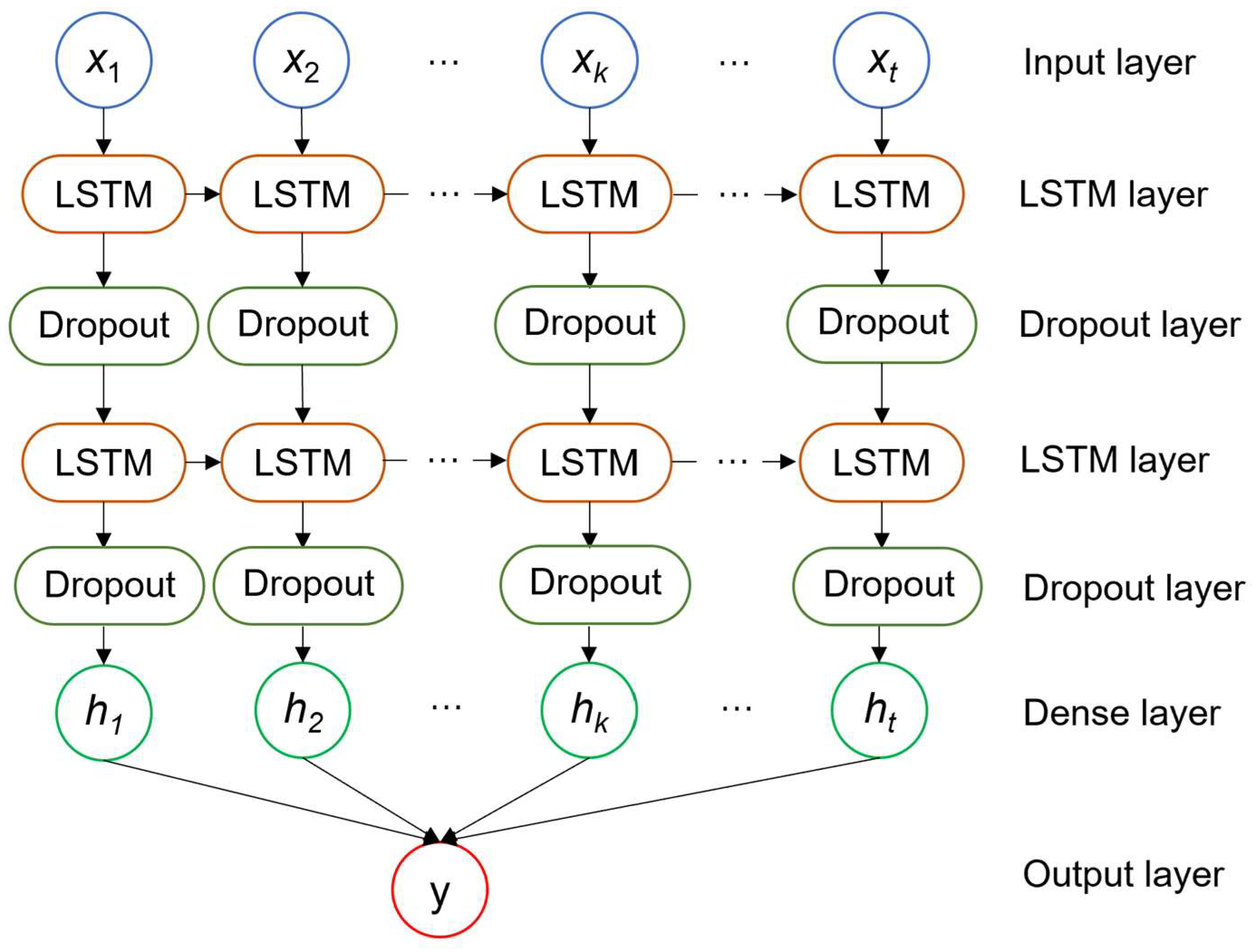
In this study, a two-layer stacked LSTM model was built on the Keras framework to construct a classifier to identify agricultural abandoned land (Figure 7). The time series of σ0VV, σ0VH, σ0VH/σ0VV, H, A and α ¯ , as well as the VGG16-based spatial features, were normalized to a range of 0 to 1, based on their maximum and minimum values. To evaluate the performance of different feature combinations in identifying abandoned land, several groups of experiments were conducted using these features. The LSTM model parameters in this study included n_hidden, n_length and n_feature, which represent the number of hidden neurons, the length of time series observations and the number of input features, respectively. In this study, n_hidden was set to 32 after conducting numerous experiments, and n_length was set to 30 based on the observation times of Sentinel-1 SAR data. After conducting multiple trial experiments, the learning_rate parameter was set to 0.0001, and the number of iteration epochs was set to 700 during the model training process. Each LSTM layer was followed by a dropout layer with the drop rate of 0.4 in order to avoid overfitting. After the stacked LSTM layers, a dense layer was added with the Softmax activation function to transform the output possibility into one of three categories: abandoned land, double-season paddy rice or other crop types. In this study, the loss function of the LSTM model was ‘sparse_categorical_crossentropy’. The optimizer was the gradient-based optimization algorithm ‘Adam’. The kernel initializer was ‘glorot_uniform’, the recurrent initializer was ‘orthogonal’, and the bias initializer was ‘zeros’.

4. Results and Discussion

4.1. Temporal Profiles of Features for Abandoned Land and Crops

Figure 8 illustrates the temporal profiles of NDVI, σ0VV, σ0VH, H, A and α ¯ for abandoned land and other dominant crop types, including double-season rice, maize, peanut and triple-season crops. These temporal profiles were obtained by averaging the feature values of the samples for each class. To better exhibit the temporal characteristics of abandoned land, the first and third quantile values were obtained using the training samples and are presented in the plots.
As illustrated in Figure 8, the temporal variations in the NDVI clearly reflect the changes in vegetation phenology. The NDVI temporal profile for abandoned land presents a bell shape with a slow growth rate and reaches the peak value between July and September throughout the year. The variations in the NDVI temporal profiles for crops reflect the growth, development and senescence processes. The NDVI reaches its peak value during the vigorous growth period and is at its lowest value during the aging phase. For example, the NDVI temporal profile for double-season rice is characterized by two peaks, one in mid-May and the other in late September, corresponding to two peak growing seasons, and the NDVI value reaches its lowest in late July due to the harvesting of early-season rice. The NDVI temporal profile of triple-season crops presents three peaks throughout the year.
Generally, the temporal profiles of σ0VV and σ0VH for abandoned land show less variability than those of other classes. The temporal profiles of σ0VV and σ0VH for double-season rice exhibit two valley points, indicating the stages of rice transplanting when the paddy field is irrigated with a lot of water. Compared to the NDVI, the temporal profiles of σ0VV and σ0VH appear to be more irregular and cannot directly reflect the phenological characteristics of vegetation. This is because the radar backscattering signals are affected by various factors, such as soil moisture, surface roughness and volume scattering, which can lead to ambiguity in the monitoring of the vegetation.
The polarimetric parameters H, A and α ¯ reflect the structural characteristics of vegetation, such as the orientation, density and size distribution of scatters, which are sensitive to the vegetation growth stage. The temporal profiles of H, A and α ¯ for the dominant crop types exhibit similar seasonal variations as the NDVI. Their temporal profiles exhibit one or more peaks throughout the year and can effectively demonstrate the phenological stages during the growth season. During the crop growth season, the temporal variations in H and α ¯ show a nearly synchronous trend with the NDVI, and the temporal trend of A is opposite to that of H and α ¯ . The abandoned land, on the other hand, does not have a distinct growth peak stage and shows smaller temporal variations throughout the year. Overall, compared to σ0VV and σ0VH, the time series of the polarimetric parameters have an advantage in exhibiting the phenological changes in vegetation and have greater potential in distinguishing abandoned land from cultivated cropland.

4.2. Optimal VGG16-Based Spatial Features

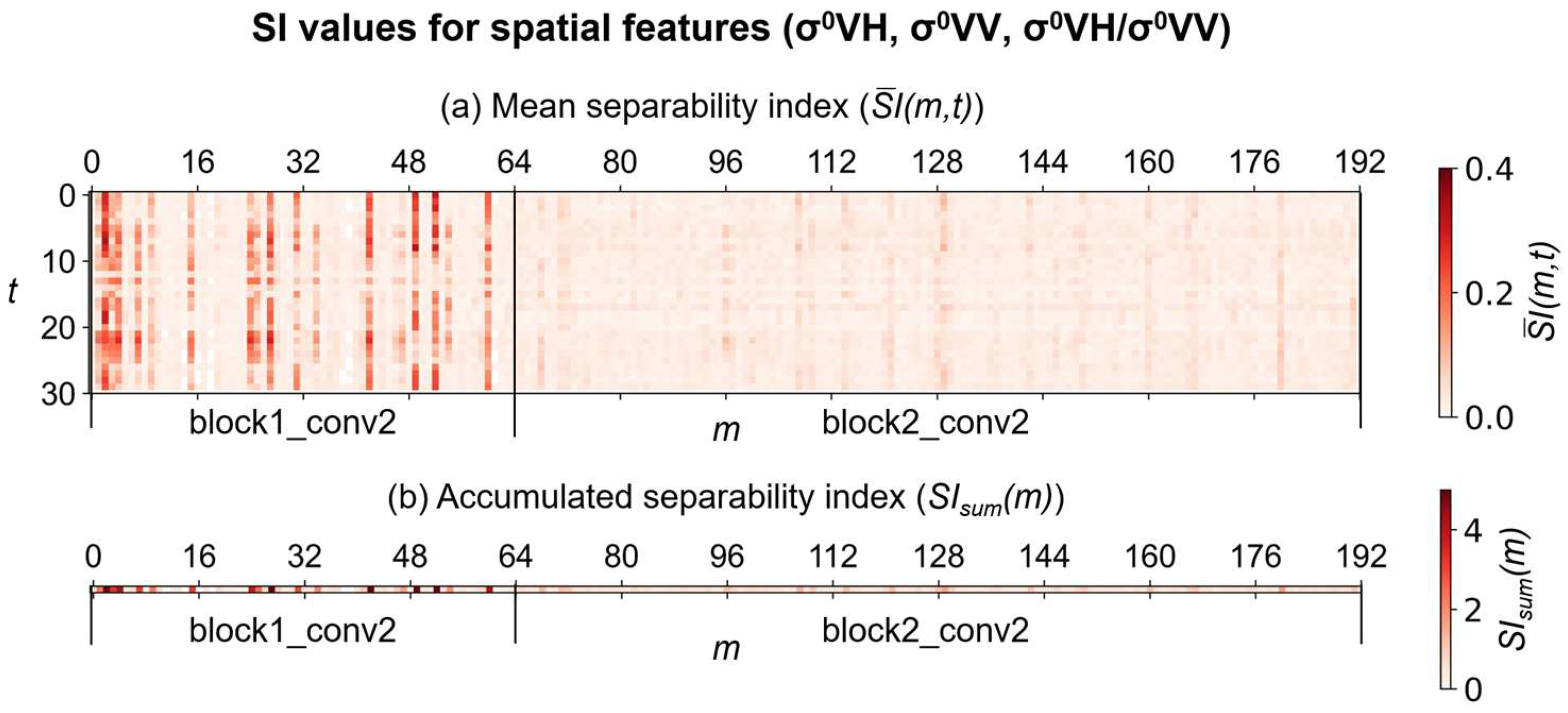
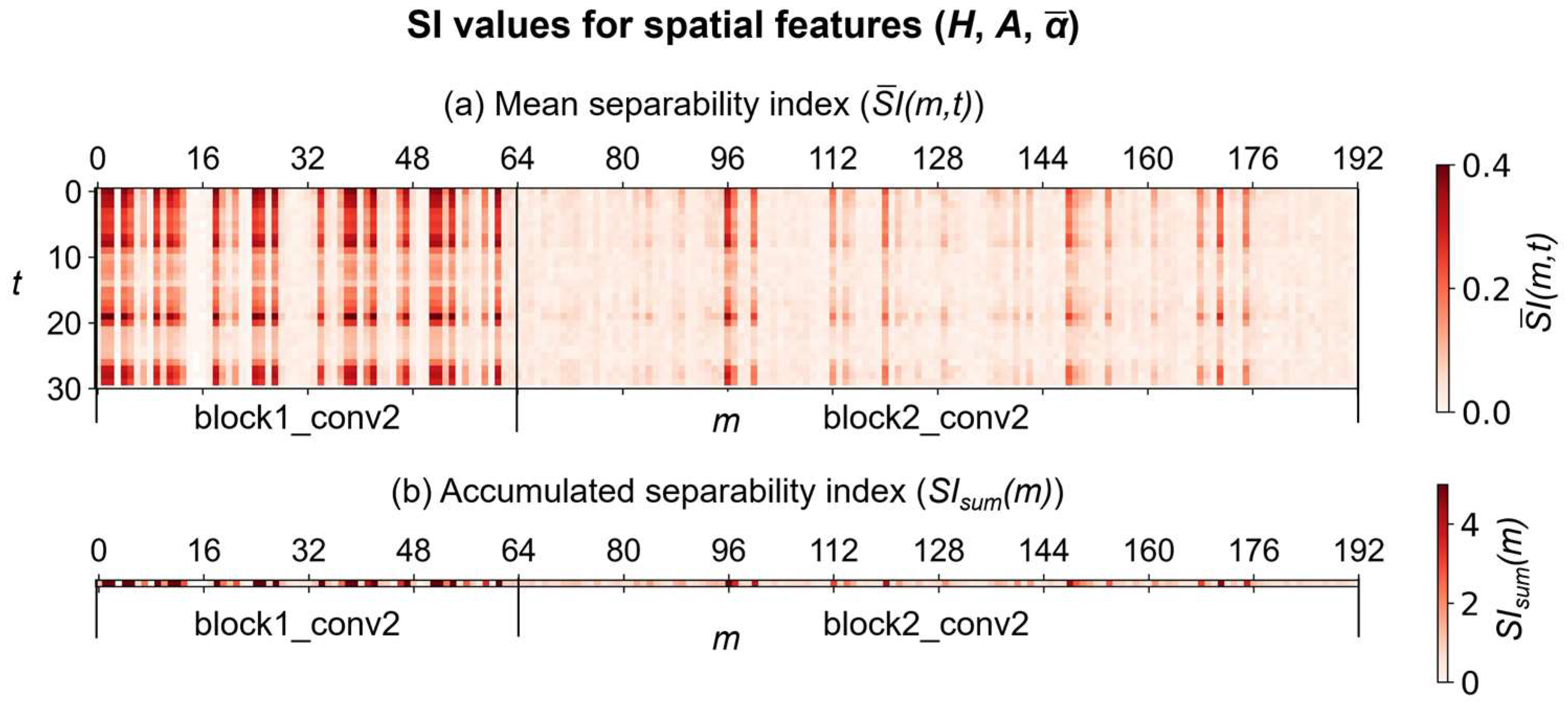
Figure 9 and Figure 10 illustrate the calculated SI values of the spatial features derived from the backscattering features and polarimetric parameters, respectively. The values of the S I ¯ for each feature at a given moment are displayed in each grid of Figure 9a and Figure 10a. Figure 9b and Figure 10b show the SIsum values, which indicate the overall ability of a feature to differentiate abandoned land by taking all moments into account.
On the whole, the spatial features of polarimetric parameters have higher capabilities in distinguishing abandoned land from other types. The spatial features from the convolutional layer ‘block1_conv2’ outperform those from the deeper convolutional layer ‘block2_conv2’. Out of the 64 features in the ‘block1_conv2’ layer derived from σ0VH, σ0VV and σ0VH/σ0VV, most of them have limited effectiveness in differentiating abandoned land from other classes (Figure 9a). The 128 features in the ‘block2_conv2’ layer have been found to have low SIsum values and are less effective in distinguishing abandoned land from other classes (Figure 9b). Regarding the 64 features in the ‘block1_conv2’ layer derived from H, A and α ¯ , nearly half of them demonstrate good performance in identifying abandoned land (Figure 10a). Several spatial features in the deeper convolutional ‘block2_conv2’ layer derived from H, A and α ¯ also present outstanding performance in distinguishing abandoned land from other classes. It can be found that the 9th and 20th phases in the multitemporal observations exhibit the best performance in distinguishing abandoned land from other classes. The ninth phase occurs on 15 April, which is during the cultivation period in spring, while the 20th phase occurs on 25 August, during the cultivation period in late summer. It is indicated that early farming activities such as sowing, plowing and flood irrigation may play a crucial role in distinguishing abandoned land from non-abandoned land.
Based on the SIsum values, 30 spatial features with SIsum values higher than 4.0 were selected for classification from the total 384 spatial features. Out of these 30 spatial features, 24 were derived from H, A and α ¯ , out of which 20 features were obtained from the ‘block1_conv2’ layer of H, A and α ¯ . The remaining six features were derived from the backscattering coefficients using the convolutional kernels of the VGG16 network.

4.3. Accuracy Comparison Based on Different Feature Combinations

This study compared the performance of different feature combinations for classification using the LSTM model. The features included backscattering features, polarimetric decomposition features and VGG16-based spatial features. Overall, five classifications were produced. Their performance was evaluated using a validation sample dataset consisting of 709 abandoned land samples, 623 double-season rice samples and 567 samples of other crop types. The confusion matrices for the five different classifications based on various feature combinations are shown in Table 2. In the confusion matrices, the producer’s accuracy (PA) measures the proportion of actual positive samples (e.g., abandoned land) that are correctly identified by the classifier, while the user’s accuracy (UA) measures the proportion of positive samples identified by the classifier that are true positives.
When using the backscattering coefficients σ0VH, σ0VV and σ0VH/σ0VV for classification, the PA was 84.34% for abandoned land and 86.84% for double-season rice, and the UA was 79.95% for abandoned land and 86.56% for double-season rice. Compared to the backscattering features, the polarimetric parameters H, A, α ¯ achieved higher accuracy for abandoned land. Specifically, the PA for abandoned land was 85.75%, and the UA was 80.74%. The combination of backscattering features and polarimetric parameters achieved better classification performance, with the PA of 86.88% for abandoned land and 88.28% for double-season rice, and the UA of 83.81% for abandoned land and 89.72% for double-season rice. This is because the polarimetric features could reflect the information about the scattering mechanism, which could not be provided by the backscattering features. Specifically, entropy measured the randomness of the scatterer, anisotropy indicated the relative importance between the secondary scattering mechanisms, and the mean alpha angle represented the scattering mechanism type in the scattering medium.
Similarly, combining the selected 30 VGG16-based spatial features with the backscattering features also improved the classification performance. Specifically, the PA reached 86.74% for abandoned land and 87.00% for double-season rice, and the UA reached 82.66% for abandoned land and 87.56% for double-season rice. Furthermore, the combination of backscattering features, polarimetric parameters and the selected 30 VGG16-based spatial features led to further improvements in classification performance. The PA increased to 88.29% for abandoned land and 89.25% for double-season rice, while the UA increased to 84.03% for abandoned and 86.20% for double-season rice. The importance of these features and their correlation coefficients was evaluated and is shown in Appendix A.
Based on the classification results, the following findings can be drawn. The performance of backscattering features of SAR data in identifying abandoned land is relatively moderate. The polarimetric parameters perform better than the backscattering features for abandoned land identification. Incorporating polarimetric parameters or VGG16-based spatial features with backscattering features can improve the classification accuracy. The combination of all three feature groups (backscattering, polarimetric and spatial features) achieves the highest classification performance.
The misclassification of the model might arise from the following factors. First, in Jiexi County, which is located in the subtropical monsoon zone, the crop types are diverse. However, only double-season rice was classified due to the limitations of the samples, and other crops such as maize and peanut were grouped together under the category of ‘other crops’, which increased the uncertainty of classification. Second, parcels abandoned within a short time are generally covered by grasses and weeds and have low vegetation cover. Parcels that have been abandoned for a long time are generally covered by shrubs or trees and have high vegetation cover. The diversity of natural vegetation in abandoned land led to various SAR signals, also causing the misclassification of the model.

4.4. Mapping of Abandoned Land in Jiexi County

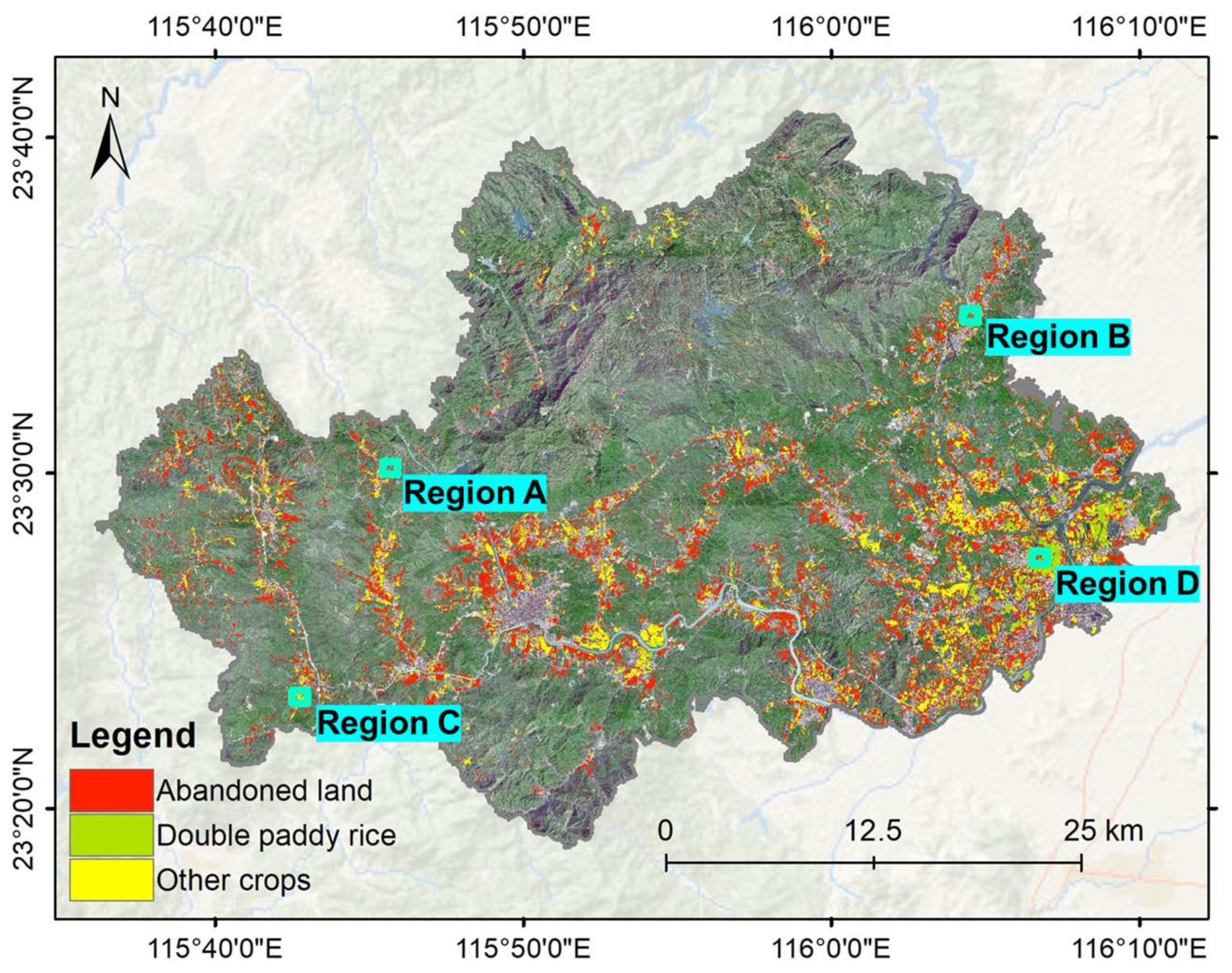
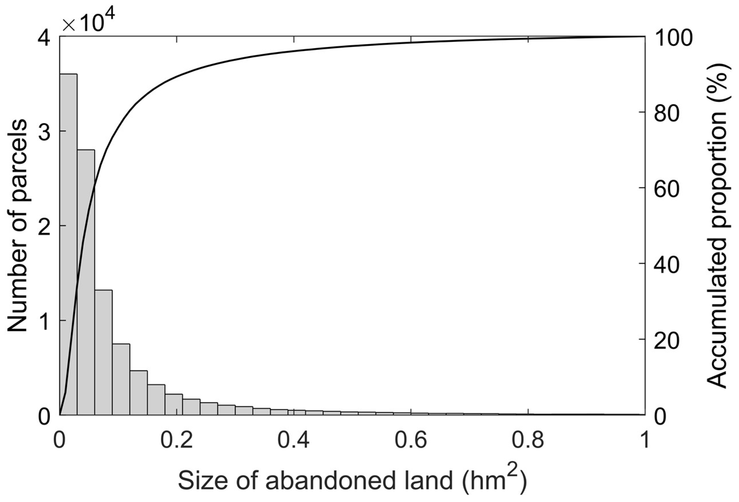
Based on the analysis of the performance of feature combinations, the backscattering features, polarimetric parameters and the 30 selected VGG16-based spatial features were combined to train the LSTM classifier. In the study area, the farmland parcel objects were classified into three categories: abandoned land, double-season paddy rice and other crops. Figure 11 shows the spatial distribution of abandoned land and non-abandoned land in Jiexi County. The abandoned lands were widely distributed across the study area. The number of abandoned land parcels was found to be 38,952. In general, abandoned lands in mountainous areas are larger and have a more contiguous distribution, whereas those in plain areas are typically smaller and more scattered. Figure 12 displays the histogram of abandoned land sizes and their cumulative proportions. The plot indicates that over 80% of the abandoned land areas are smaller than 0.12 hm2, with only approximately 3% larger than 0.5 hm2. The largest abandoned land area observed is approximately 23.3 hm2.
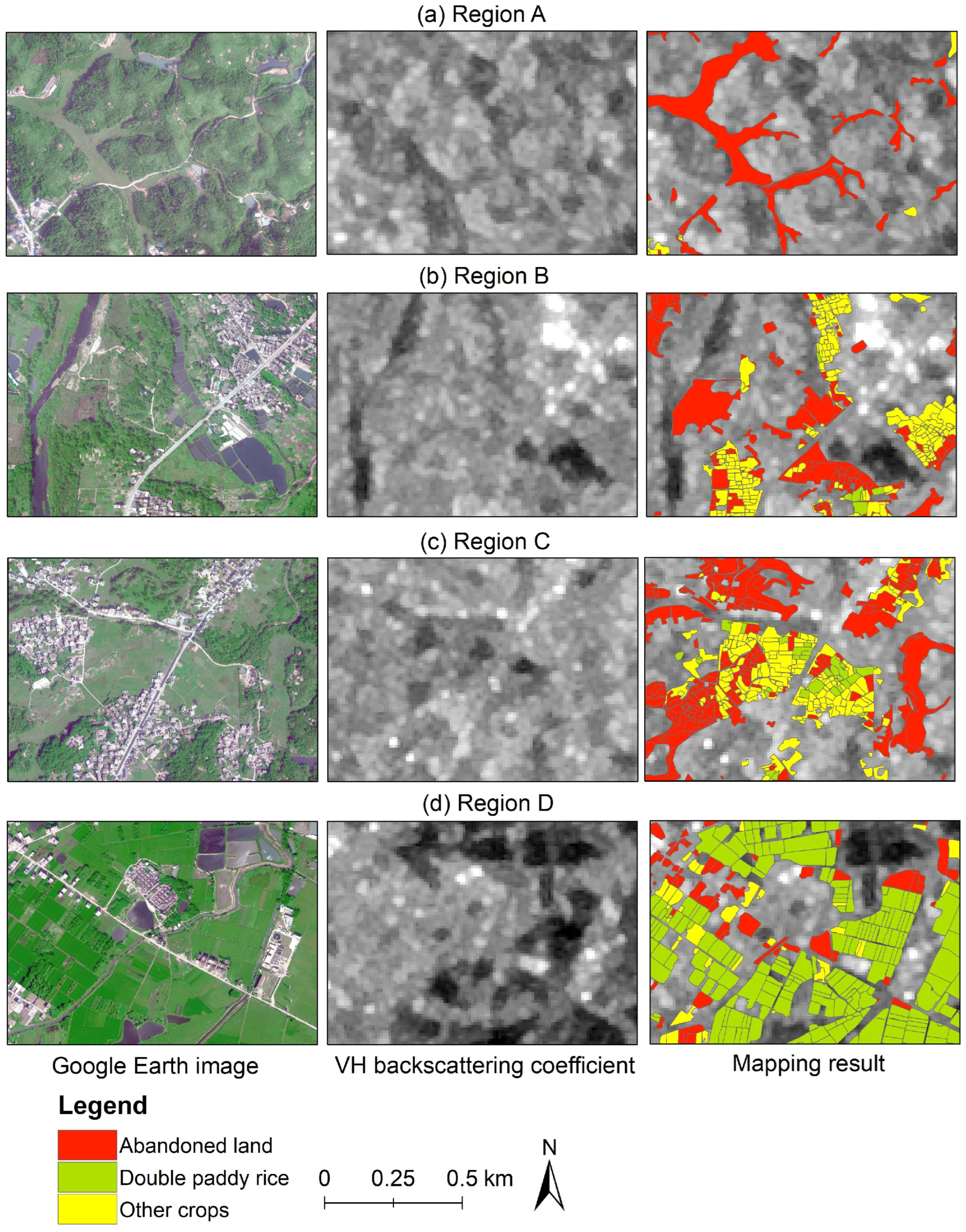
Figure 13 illustrates the mapping results for four selected regions and the corresponding high-resolution Google Earth images for reference. Region A is situated in the northwest of Jiexi County and characterized by mountainous terrain. Farmlands in this region are located in flat valleys among mountains, and almost all of them are abandoned. The abandoned lands are characterized by an irregular shape and continuous distribution in space with blurred boundaries. The Google Earth image shows that these lands are covered by natural grasslands with a low vegetation cover fraction, indicating that they have been abandoned for a long time. Regions B and C are flat areas near towns, with diverse land use types, including croplands, forest lands, orchards and residential areas. In these regions, abandoned lands are scattered among cultivated croplands, with most of them being small-sized, while a few are larger than 2 hm2. Region D, situated in the Rongjiang alluvial plain, has a flat and open terrain with an altitude of below 20 m. This region is the main rice-producing area, where paddy rice can be cropped twice a year. Compared to Regions A, B and C, farmlands in this region are rarely abandoned. The few abandoned lands are mostly distributed in the edges of cultivated areas and are covered by trees and shrubs.

4.5. Discussion of the Computational Cost

Compared to the traditional machine learning methods, such as random forest or support vector machine, the deep learning methods cost more time, which can be directly determined by the model parameter epochs. The setting of epochs must consider the value of the learning rate. If the learning rate is too low, it will require more time in the training process. If the learning rate is too high, the model will be unable to converge. In this study, the number of iterations (epochs) was set to 700 under a learning rate of 0.0001 for the stability of model convergence, and the model training process required 554 s. Moreover, we tested other values of the learning rate and adjusted the epochs at the same time to reach the status of model convergence. When the learning rate was 0.0005 and the number of iterations was 200, the model training process required 163 s. When the learning rate was 0.001 and the number of iterations was 100, the model training process required 83 s, but the loss curves presented oscillation.

5. Conclusions

This study proposed a new method to identify abandoned land based on the spatiotemporal features from PolSAR data via deep learning methods. It innovatively combined the backscattering coefficients, polarimetric parameters and convolution-based spatial features to identify abandoned land and produced higher classification performance.
In the proposed method, the backscattering coefficients σ0VH, σ0VV and polarimetric parameters H, A and α ¯ were first extracted from PolSAR SLC products, and time series of these features were constructed. The temporal profiles showed that the polarimetric parameters H, A and α ¯ were more effective than the backscattering coefficients σ0VH and σ0VV in depicting the vegetation phenological processes. Then, based on the VGG16 convolutional network, high-dimensional spatial features were extracted from both the backscattering coefficients and the polarimetric parameters. After applying the separability index, 30 features were selected as the most effective in distinguishing abandoned land from other classes. Among the selected 30 spatial features, 24 of them were derived from the polarimetric parameters H, A and α ¯ , and 20 of them were derived from the ‘block1_conv2’ layer of H, A and α ¯ . This indicated that spatial features from the shallow convolutional layer derived from polarimetric parameters were more useful to capture the structural characteristics of vegetation. After this, LSTM classifications were conducted using the time series of backscattering features, polarimetric parameters, the selected VGG16-based spatial features and their combinations. The performance of these feature combinations in abandoned land identification was evaluated using a large number of samples.
The results showed that the polarimetric parameters derived from Cloude–Pottier decomposition performed better than the backscattering coefficients in identifying abandoned land. Additionally, the use of VGG16-based spatial features could provide complementary information about the spatial structure of the land cover, which had the capability to boost the classification accuracy. Combining the backscattering features, polarimetric parameters and VGG16-based spatial features produced the most precise classification result in identifying abandoned land, with the PA reaching 88.29% and the UA reaching 84.03%. In summary, this study demonstrated that the incorporation of polarimetric parameters and convolution-based spatial features could contribute to the improvement of the classification accuracy. The method has the capability of producing highly reliable abandoned land mapping in cloudy and rainy areas.
Further research can be carried out as follows. Without human intervention, abandoned lands are typically covered by natural vegetation such as grasses, weeds, shrubs and trees. The features of these different land cover types in PolSAR data may vary due to the diversity of the vegetation structure. It is important to conduct more analyses of PolSAR features for different land cover types, for a better understanding of the characteristics of various vegetation types and to further improve the accuracy of abandoned land identification. In addition, due to the limited number of validation samples, this study only classified croplands into three categories: abandoned land, double-season rice and other crops. Further analyses are necessary to determine which crop types are easily misclassified as abandoned land.

Author Contributions

Conceptualization, Y.Y.; methodology, Y.Y. and Y.Z.; validation, W.X. and H.W.; investigation, Q.H.; resources, T.W.; writing—original draft preparation, Y.Y.; writing—review and editing, Q.H.; supervision, J.L.; project administration, Z.W.; funding acquisition, Y.Y. All authors have read and agreed to the published version of the manuscript.

Funding

This research was supported by the Key Laboratory of Natural Resources Monitoring in Tropical and Subtropical Area of South China, Ministry of Natural Resources (No. 2022NRM004).

Conflicts of Interest

The authors declare no conflict of interest.

Appendix A

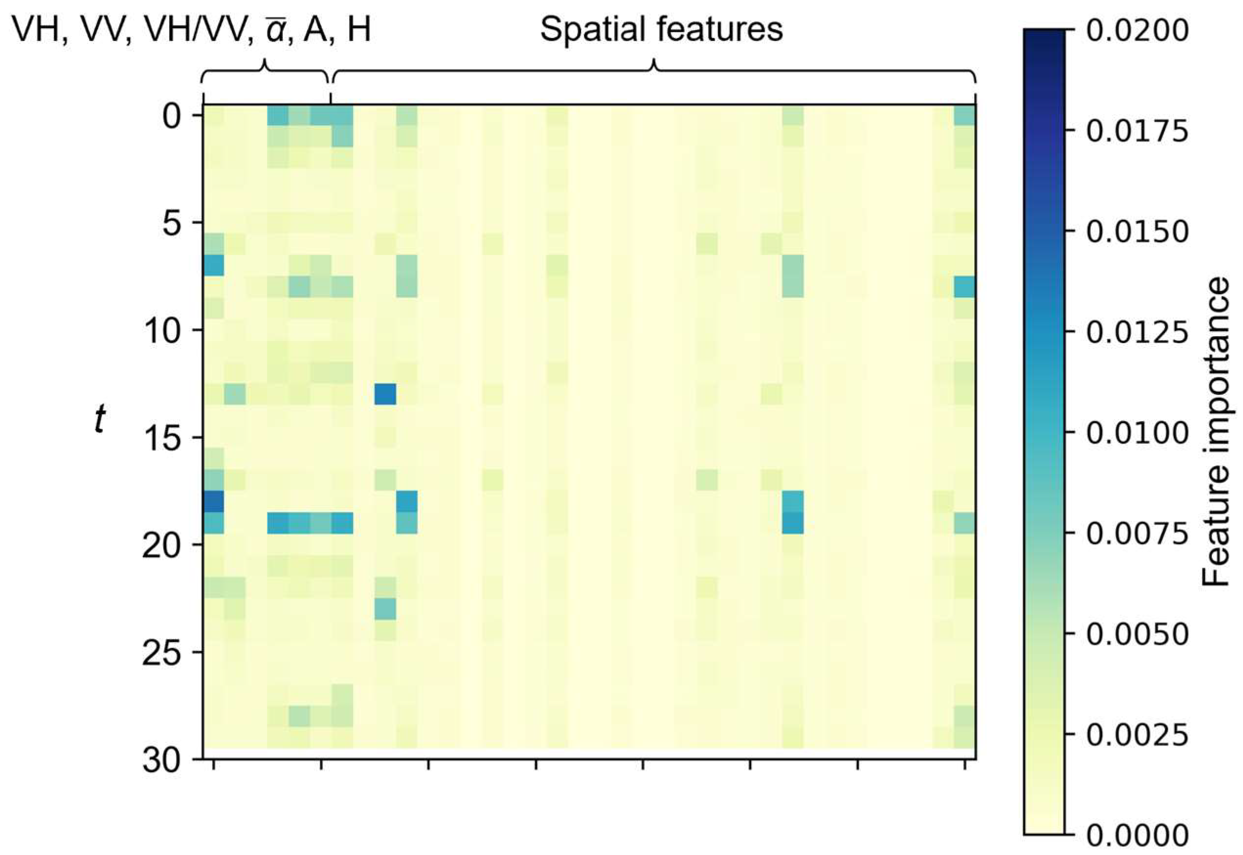
The importance of the adopted features (σ0VH, σ0VV, σ0VH/σ0VV, H, A, α ¯ and the selected spatial features) was evaluated using the random forest algorithm. The importance ranking result is shown below (Figure A1). It shows that H, A, α ¯ and σ0VH play important roles in classification, while σ0VV and σ0VH/σ0VV have lower importance. Four spatial features exhibit high importance as well. One the whole, some observation phases are quite important for classification, including mid-winter (9 January, 21 January), early spring (22 March–15 April) and mid-summer (20 July–13 August).
Figure A1. The importance of features (σ0VH, σ0VV, σ0VH/σ0VV, H, A, α ¯ and spatial features) at each observation time.
Remotesensing 15 03942 g0a1
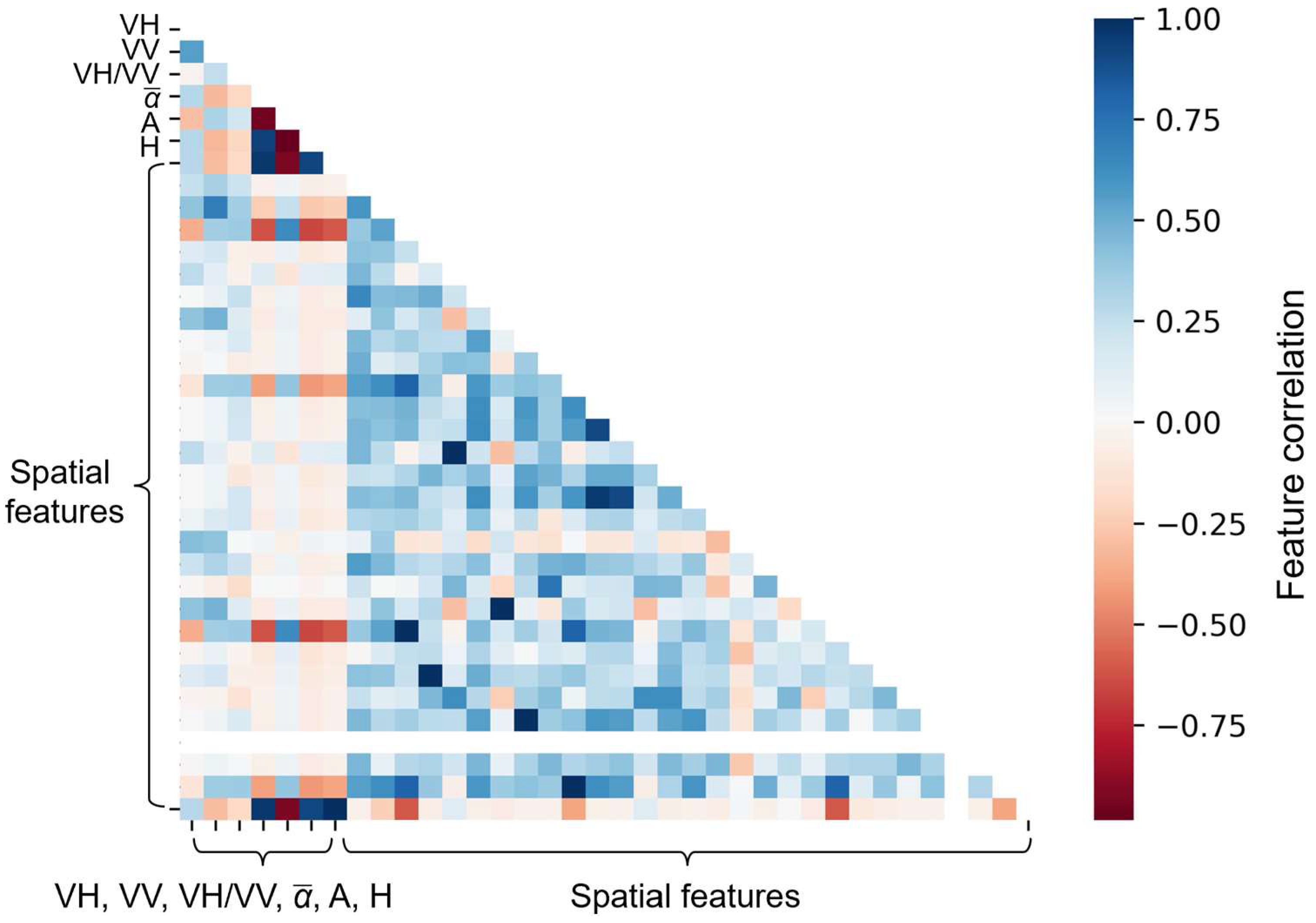
The correlation coefficients between the input features were calculated and are shown in Figure A2, where each grid was calculated as the mean value of the coefficients considering all observations. It shows that the correlation coefficient between σ0VH and σ0VV was 0.56. Polarimetric parameters had strong correlations with each other. Specifically, H and α ¯ presented a strong positive correlation, with the correlation coefficient of 0.94, while A had a strong negative correlation with them. The correlation coefficient between A and H was −0.99, and the coefficient between A and α ¯ was −0.95. These findings are consistent with the characteristics of the temporal variations for these features (Section 4.1). Overall, there is a relatively weak correlation between the backscattering coefficients and polarimetric parameters. For example, the correlation coefficient between σ0VH and H was 0.29. Generally, the correlations between the spatial features and the backscattering coefficients and polarimetric parameters were weak. This explains why the combination of backscattering coefficients and polarimetric parameters could improve the classification performance.
Figure A2. Correlation coefficients between the features (σ0VH, σ0VV, σ0VH/σ0VV, H, A, α ¯ and spatial features).
Remotesensing 15 03942 g0a2

References

  1. Kuemmerle, T.; Radeloff, V.C.; Perzanowski, K.; Hostert, P. Cross-border comparison of land cover and landscape pattern in Eastern Europe using a hybrid classification technique. Remote Sens. Environ. 2006, 103, 449–464. [Google Scholar] [CrossRef]
  2. Aide, T.M.; Grau, H.R. Globalization, migration, and Latin American ecosystems. Science 2004, 305, 1915–1916. [Google Scholar] [CrossRef]
  3. Cramer, V.A.; Hobbs, R.J.; Standish, R.J. What’s new about old fields? Land abandonment and ecosystem assembly. Trends Ecol. Evol. 2008, 23, 104–112. [Google Scholar] [CrossRef]
  4. Ruiz-Flan˜o, P.; Garci´a-Ruiz, J.M.; Ortigosa, L. Geomorphological evolution of abandoned fields. A case study in the Central Pyrenees. CATENA 1992, 19, 301–308. [Google Scholar] [CrossRef]
  5. Stanchi, S.; Freppaz, M.; Agnelli, A.; Reinsch, T.; Zanini, E. Properties, best management practices and conservation of terraced soils in Southern Europe (from Mediterranean areas to the Alps): A review. Quat. Int. 2012, 265, 90–100. [Google Scholar] [CrossRef] [Green Version]
  6. Fischer, J.; Hartel, T.; Kuemmerle, T. Conservation policy in traditional farming landscapes. Conserv. Lett. 2012, 5, 167–175. [Google Scholar] [CrossRef] [Green Version]
  7. Meijninger, W.; Elbersen, B.; van Eupen, M.; Mantel, S.; Ciria, P.; Parenti, A.; Sanz, M.; Ortiz, P.; Acciai, M.; Monti, A. Identification of early abandonment in cropland through radar-based coherence data and application of a Random-Forest model. GCB Bioenergy 2022, 14, 735–755. [Google Scholar] [CrossRef]
  8. Goga, T.; Feranec, J.; Bucha, T.; Rusnák, M.; Sačkov, I.; Barka, I.; Kopecká, M.; Papčo, J.; Oťaheľ, J.; Szatmári, D.; et al. A review of the application of remote sensing data for abandoned agricultural land identification with focus on central and eastern Europe. Remote Sens. 2019, 11, 2759. [Google Scholar] [CrossRef] [Green Version]
  9. Yusoff, N.M.; Muharam, F.M.; Khairunniza-Bejo, S. Towards the use of remote-sensing data for monitoring of abandoned oil palm lands in Malaysia: A semi-automatic approach. Int. J. Remote Sens. 2017, 38, 432–449. [Google Scholar] [CrossRef]
  10. Prishchepov, A.V.; Radeloff, V.C.; Dubinin, M.; Alcantara, C. The effect of Landsat ETM/ETM+ image acquisition dates on the detection of agricultural land abandonment in Eastern Europe. Remote Sens. Environ. 2012, 126, 195–209. [Google Scholar] [CrossRef]
  11. Alcantara, C.; Kuemmerle, T.; Prishchepov, A.V.; Radeloff, V.C. Mapping abandoned agriculture with multi-temporal MODIS satellite data. Remote Sens. Environ. 2012, 124, 334–347. [Google Scholar] [CrossRef]
  12. Estel, S.; Kuemmerle, T.; Alcántara, C.; Levers, C.; Prishchepov, A.; Hostert, P. Mapping farmland abandonment and recultivation across Europe using MODIS NDVI time series. Remote Sens. Environ. 2015, 163, 312–325. [Google Scholar] [CrossRef]
  13. Wei, Z.; Gu, X.; Sun, Q.; Hu, X.; Gao, Y. Analysis of the Spatial and Temporal Pattern of Changes in Abandoned Farmland Based on Long Time Series of Remote Sensing Data. Remote Sens. 2021, 13, 2549. [Google Scholar] [CrossRef]
  14. Löw, F.; Fliemann, E.; Abdullaev, I.; Conrad, C.; Lamers, J.P.A. Mapping abandoned agricultural land in Kyzyl-Orda, Kazakhstan using satellite remote sensing. Appl. Geogr. 2015, 62, 377–390. [Google Scholar] [CrossRef]
  15. Wang, C.; Gao, Q.; Wang, X.; Yu, M. Spatially differentiated trends in urbanization, agricultural land abandonment and reclamation, and woodland recovery in Northern China. Sci. Rep. 2016, 6, 37658. [Google Scholar] [CrossRef] [PubMed] [Green Version]
  16. Dara, A.; Baumann, M.; Kuemmerle, T.; Pflugmacher, D.; Rabe, A.; Griffiths, P.; Hölzel, N.; Kamp, J.; Freitag, M.; Hostert, P. Mapping the timing of cropland abandonment and recultivation in northern Kazakhstan using annual Landsat time series. Remote Sens. Environ. 2018, 213, 49–60. [Google Scholar] [CrossRef]
  17. Campbell, J.E.; Lobell, D.B.; Genova, R.C.; Field, C.B. The global potential of bioenergy on abandoned agriculture lands. Environ. Sci. Technol. 2008, 42, 5791–5794. [Google Scholar] [CrossRef]
  18. Zhang, M.; Li, G.; He, T.; Zhai, G.; Guo, A.; Chen, H.; Wu, C. Reveal the severe spatial and temporal patterns of abandoned cropland in China over the past 30 years. Sci. Total Environ. 2023, 857, 159591. [Google Scholar] [CrossRef]
  19. Yin, H.; Prishchepov, A.V.; Kuemmerle, T.; Bleyhl, B.; Buchner, J.; Radeloff, V.C. Mapping agricultural land abandonment from spatial and temporal segmentation of Landsat time series. Remote Sens. Environ. 2018, 210, 12–24. [Google Scholar] [CrossRef]
  20. Olsen, V.M.; Fensholt, R.; Olofsson, P.; Bonifacio, R.; Butsic, V.; Druce, D.; Ray, D.; Prishchepov, A.V. The impact of conflict-driven cropland abandonment on food insecurity in South Sudan revealed using satellite remote sensing. Nat. Food 2021, 2, 990–996. [Google Scholar] [CrossRef]
  21. Witmer, F.D.W. Detecting war-induced abandoned agricultural land in northeast Bosnia using multispectral, multitemporal Landsat TM imagery. Int. J. Remote Sens. 2008, 29, 3805–3831. [Google Scholar] [CrossRef]
  22. Milenov, P.; Vassilev, V.; Vassileva, A.; Radkov, R.; Samoungi, V.; Dimitrov, Z.; Vichev, N. Monitoring of the risk of farmland abandonment as an efficient tool to assess the environmental and socio-economic impact of the Common Agriculture Policy. Int. J. Appl. Earth Obs. Geoinf. 2014, 32, 218–227. [Google Scholar] [CrossRef]
  23. Waske, B.; Braun, M. Classifier ensembles for land cover mapping using multitemporal SAR imagery. ISPRS J. Photogramm. Remote Sens. 2009, 64, 450–457. [Google Scholar] [CrossRef]
  24. Pohl, C.; Van Genderen, J.L. Review article multisensor image fusion in remote sensing: Concepts, methods and applications. Int. J. Remote Sens. 1998, 19, 823–854. [Google Scholar] [CrossRef] [Green Version]
  25. Stefanski, J.; Kuemmerle, T.; Chaskovskyy, O.; Griffiths, P.; Havryluk, V.; Knorn, J.; Korol, N.; Sieber, A.; Waske, B. Mapping land management regimes in Western Ukraine using optical and SAR data. Remote Sens. 2014, 6, 5279–5305. [Google Scholar] [CrossRef] [Green Version]
  26. Ray, T.W.; Farr, T.G.; van Zyl, J.J. Detection of land degradation with polarimetric SAR. Geophys. Res. Lett. 1992, 19, 1587–1590. [Google Scholar] [CrossRef]
  27. McNairn, H.; Champagne, C.; Shang, J.; Holmstrom, D.; Reichert, G. Integration of optical and Synthetic Aperture Radar (SAR) imagery for delivering operational annual crop inventories. ISPRS J. Photogramm. Remote Sens. 2009, 64, 434–449. [Google Scholar] [CrossRef]
  28. Yusoff, N.M.; Muharam, F.M.; Takeuchi, W.; Darmawan, S.; Abd Razak, M.H. Phenology and classification of abandoned agricultural land based on ALOS-1 and 2 PALSAR multi-temporal measurements. Int. J. Digit. Earth 2017, 10, 155–174. [Google Scholar] [CrossRef]
  29. Xie, Q.; Wang, J.; Liao, C.; Shang, J.; Lopez-Sanchez, J.M.; Fu, H.; Liu, X. On the use of Neumann Decomposition for crop classification using multi-temporal RADARSAT-2 polarimetric SAR data. Remote Sens. 2019, 11, 776. [Google Scholar] [CrossRef] [Green Version]
  30. Ioannidou, M.; Koukos, A.; Sitokonstantinou, V.; Papoutsis, I.; Kontoes, C. Assessing the added value of Sentinel-1 PolSAR data for crop classification. Remote Sens. 2022, 14, 5739. [Google Scholar] [CrossRef]
  31. Canisius, F.; Shang, J.; Liu, J.; Huang, X.; Ma, B.; Jiao, X.; Geng, X.; Kovacs, J.M.; Walters, D. Tracking crop phenological development using multi-temporal polarimetric Radarsat-2 data. Remote Sens. Environ. 2018, 210, 508–518. [Google Scholar] [CrossRef]
  32. Zhou, Y.n.; Luo, J.; Feng, L.; Zhou, X. DCN-Based spatial features for improving parcel-based crop classification using high-resolution optical images and multi-temporal SAR data. Remote Sens. 2019, 11, 1619. [Google Scholar]
  33. Kussul, N.; Lavreniuk, M.; Skakun, S.; Shelestov, A. Deep learning classification of land cover and crop types using remote sensing data. IEEE Geosci. Remote Sens. Lett. 2017, 14, 778–782. [Google Scholar] [CrossRef]
  34. Zhang, C.; Sargent, I.; Pan, X.; Li, H.; Gardiner, A.; Hare, J.; Atkinson, P.M. Joint deep learning for land cover and land use classification. Remote Sens. Environ. 2019, 221, 173–187. [Google Scholar] [CrossRef] [Green Version]
  35. Li, Y.; Peng, C.; Chen, Y.; Jiao, L.; Zhou, L.; Shang, R. A deep learning method for change detection in synthetic aperture radar images. IEEE Trans. Geosci. Remote Sens. 2019, 57, 5751–5763. [Google Scholar] [CrossRef]
  36. Cloude, S.R.; Pottier, E. An entropy based classification scheme for land applications of polarimetric SAR. IEEE Trans. Geosci. Remote Sens. 1997, 35, 68–78. [Google Scholar] [CrossRef]
  37. Simonyan, K.; Zisserman, A. Very Deep Convolutional Networks for Large-Scale Image Recognition. In Proceedings of the ICLR 2015, San Diego, CA, USA, 7–9 May 2015. [Google Scholar]
  38. Liu, X.; Chi, M.; Zhang, Y.; Qin, Y. Classifying high resolution remote sensing images by fine-tuned VGG deep networks. In Proceedings of the IGARSS 2018—2018 IEEE International Geoscience and Remote Sensing Symposium, Valencia, Spain, 22–27 July 2018; pp. 7137–7140. [Google Scholar]
  39. Mu, Y.; Ni, R.; Zhang, C.; Gong, H.; Hu, T.; Li, S.; Sun, Y.; Zhang, T.; Guo, Y. A lightweight model of VGG-16 for remote sensing image classification. IEEE J. Sel. Top. Appl. Earth Obs. Remote Sens. 2021, 14, 6916–6922. [Google Scholar] [CrossRef]
  40. Somers, B.; Asner, G.P. Multi-temporal hyperspectral mixture analysis and feature selection for invasive species mapping in rainforests. Remote Sens. Environ. 2013, 136, 14–27. [Google Scholar] [CrossRef]
  41. Hu, Q.; Sulla-Menashe, D.; Xu, B.; Yin, H.; Tang, H.; Yang, P.; Wu, W. A phenology-based spectral and temporal feature selection method for crop mapping from satellite time series. Int. J. Appl. Earth Obs. Geoinf. 2019, 80, 218–229. [Google Scholar] [CrossRef]
  42. Hochreiter, S.; Schmidhuber, J. Long short-term memory. Neural Comput. 1997, 9, 1735–1780. [Google Scholar] [CrossRef]
  43. Tian, H.; Wang, P.; Tansey, K.; Zhang, J.; Zhang, S.; Li, H. An LSTM neural network for improving wheat yield estimates by integrating remote sensing data and meteorological data in the Guanzhong Plain, PR China. Agric. For. Meteorol. 2021, 310, 108629. [Google Scholar] [CrossRef]
  44. Portalés-Julià, E.; Campos-Taberner, M.; García-Haro, F.; Gilabert, M.A. Assessing the Sentinel-2 Capabilities to Identify Abandoned Crops Using Deep Learning. Agronomy 2021, 11, 654. [Google Scholar] [CrossRef]
Figure 1. Location of Jiexi County.
Remotesensing 15 03942 g001
Figure 2. Photos taken in the field survey. (a) Abandoned land. (b) Paddy rice. (c) Maize. (d) Peanut.
Remotesensing 15 03942 g002
Figure 3. Regions of abandoned land and non-abandoned land on Google Earth images. (ac) are images of abandoned land regions, and (df) are images of non-abandoned land regions.
Remotesensing 15 03942 g003
Figure 4. Flowchart of the abandoned land mapping method in this work.
Remotesensing 15 03942 g004
Figure 5. The backscattering coefficients of VH and VV band and Cloude–Pottier decomposition parameters (mean alpha angle, anisotropy and entropy) of Sentinel-1 data on 20 July 2020.
Remotesensing 15 03942 g005
Figure 6. The process of generating normalized composite images and spatial features for one tile with 224 × 224 pixels.
Remotesensing 15 03942 g006
Figure 7. The architecture of the LSTM model for abandoned land identification.
Remotesensing 15 03942 g007
Figure 8. Temporal profiles of features for abandoned land and dominant crop types including double-season rice, maize, peanut and triple-season crops. (a) NDVI, (b) σ0VV, (c) σ0VH, (d) H, (e) A and (f) α ¯ . The shaded areas refer to ranges between the first quantile (Q1) and third quantile (Q3) of each index for abandoned land.
Remotesensing 15 03942 g008
Figure 9. Separability indexes of VGG16-based spatial features derived from the composite three-band images of σ0VH, σ0VV and σ0VH/σ0VV. (a) Matrix of mean separability index ( S I ¯ ) for abandoned land and the other classes. Each grid in the matrix represents the S I ¯ (m,t) value, which refers to the separability index of the m-th feature on t-th observation. (b) Matrix of accumulated separability index (SIsum) values for each feature.
Remotesensing 15 03942 g009
Figure 10. Separability indexes of VGG16-based spatial features derived from the composite three-band images of H, A and α ¯ . (a) Matrix of mean separability index ( S I ¯ ) for abandoned land and the other classes. Each grid in the matrix represents the S I ¯ (m,t) value, which refers to the separability index of the m-th feature on t-th observation. (b) Matrix of accumulated separability index (SIsum) values for each feature.
Remotesensing 15 03942 g010
Figure 11. The spatial distribution of abandoned lands and non-abandoned lands (including double-season paddy rice and other crops) in Jiexi County. Four typical regions were selected from the study area, and the detailed maps of these regions are shown in Figure 12.
Remotesensing 15 03942 g011
Figure 12. Histogram of abandoned land sizes and their cumulative proportions.
Remotesensing 15 03942 g012
Figure 13. Detailed mapping results of four selected regions, the high-resolution Google Earth images and the VH backscattering coefficient images.
Remotesensing 15 03942 g013
Table 1. Information of the Sentinel-1 images used in this study.
Date Date
19 January 2021168 July 2021
221 January 20211720 July 2021
32 February 2021181 August 2021
414 February 20211913 August 2021
526 February 20212025 August 2021
610 March 2021216 September 2021
722 March 20212218 September 2021
83 April 20212330 September 2021
915 April 20212412 October 2021
1027 April 20212524 October 2021
119 May 2021265 November 2021
1221 May 20212717 November 2021
132 June 20212829 November 2021
1414 June 20212911 December 2021
1526 June 20213023 December 2021
Table 2. Confusion matrices for the LSTM classification under different feature combinations. PA, UA and OA represent the producer’s accuracy, user’s accuracy and overall accuracy, respectively.
Feature CombinationReferenceClassificationPA
Abandoned LandDouble RiceOther Crops
σ0VH, σ0VV, σ0VH/σ0VVAbandoned land598228984.34%
Double rice145416886.84%
Other crops1366236965.08%
UA79.95%86.56%70.15%
OA: 79.41%, Kappa: 0.69
H, A, α ¯ Abandoned land60869585.75%
Double rice175406686.68%
Other crops1286637365.78%
UA80.74%88.24%69.85%
OA: 80.09%, Kappa: 0.70
σ0VH, σ0VV, σ0VH/σ0VV,
H, A, α ¯
Abandoned land61698486.88%
Double rice165505788.28%
Other crops1035441072.31%
UA83.81%89.72%74.41%
OA: 82.99%, Kappa: 0.74
σ0VH, σ0VV, σ0VH/σ0VV,
VGG16-based spatial features
Abandoned land615167886.74%
Double rice125426987.00%
Other crops1176138968.61%
UA82.66%87.56%72.57%
OA: 81.41%, Kappa: 0.72
σ0VH, σ0VV, σ0VH/σ0VV,
H, A, α ¯ ,
VGG16-based spatial features
Abandoned land626186588.29%
Double rice155565289.25%
Other crops1047139269.14%
UA84.03%86.20%77.01%
OA: 82.89%, Kappa: 0.74
Disclaimer/Publisher’s Note: The statements, opinions and data contained in all publications are solely those of the individual author(s) and contributor(s) and not of MDPI and/or the editor(s). MDPI and/or the editor(s) disclaim responsibility for any injury to people or property resulting from any ideas, methods, instructions or products referred to in the content.