Cross-Domain Automatic Modulation Classification Using Multimodal Information and Transfer Learning

Abstract

Automatic modulation classification (AMC) based on deep learning (DL) is gaining increasing attention in dynamic spectrum access for 5G/6G wireless communications. However, inconsistent feature parameters between the training (source) and testing (target) data lead to performance degradation or even failure of existing DL-based AMC. The primary reason for this is the difficulty in obtaining sufficient labeled training data in the target domain. Therefore, we propose a novel cross-domain AMC algorithm based on multimodal information and transfer learning, utilizing abundant unlabeled target domain data. We achieve complementary gains by fusing multimodal information such as amplitude, phase, and spectrum, which are used to train a network. Additionally, we apply domain adversarial neural network technology from transfer learning to learn from a large number of unlabeled data samples in the target domain to address the issue of decreased accuracy in cross-domain AMC caused by differences in sampling rate, signal-to-noise ratio, and channel variations. Furthermore, we introduce class weight weighting and entropy weighting to solve the partial domain adaptation problem, considering that the target domain has fewer modulation signal classes than the source domain. Experimental results on two designed modulation datasets demonstrate improved performance gains, thus validating the effectiveness of the proposed method.

1. Introduction

Deep learning (DL) for automatic modulation classification (AMC) is gaining increasing attention in cognitive radio and spectrum sensing technologies. This approach can support the refarming of spectrum resources with low utilization, which is crucial for developing 5G/6G wireless communications. AMC [1] refers to the identification of the modulation schemes of an unknown signal received with limited prior knowledge for use in scenarios such as electromagnetic situational awareness [2], cognitive radio [3], dynamic spectrum access [4], and interference identification [5]. Classical AMC methods can be divided into maximum-likelihood hypothesis testing based on decision theory and pattern recognition based on feature extraction [6]. The likelihood ratio test methods are optimal in terms of Bayesian estimation for their classification results. However, the identification process requires higher prior knowledge and has stringent hypothesis constraints. Moreover, a suitable likelihood ratio function for different modulation schemes is required [7,8], and the calculation complexity of the likelihood ratio function is high. Therefore, pattern recognition based on feature extraction methods [9,10] is widely used in practice. However, owing to ever-emerging complex signals and increasingly crowded electromagnetic environments, feature extraction methods face several challenges, including difficulty setting manual feature thresholds and achieving optimal combinations subjectively, resulting in poor adaptability to complex environments, complex modulation schemes, and similar modulation schemes. Furthermore, these methods have low classification accuracy under low signal-to-noise ratio (SNR) conditions.

To address these challenges, recently, deep learning (DL) has been applied to AMC. DL methods do not require manual design or the extraction of signal features. Neural networks can adaptively extract and infer modulation signal features that are more robust and generalizable. The mainstream DL technologies include convolutional neural networks (CNN), recurrent neural networks (RNN) [11], and some hybrid models, which show superior performance over classical methods in AMC.

Currently, most AMC approaches obtain experimental datasets through three main methods: MATLAB/GNU radio simulation, data collection in a single real scenario, and direct use of publicly available datasets, such as RML 2016 and 2018 [12]. A part of the generated/sampled/publicly obtained sample data is used to train neural networks, and another part is used to test and verify the method’s effectiveness. In the research process, optimization is primarily conducted on the data or the neural network model to enhance classification performance. Appropriate data preprocessing can maximize the differences between different modulation schemes, thus ensuring improved classification by the neural network. The network model and hyperparameters can also be fine-tuned to AMC tasks.

However, existing DL-based AMC algorithms often encounter specific problems and challenges in practical applications. First, many studies predominantly rely on monomodal information from a single depicting dimension, disregarding the complementarities that multimodal information can generate to better adapt to complex scenarios with different SNR and channel variations. Based on signal representation and preprocessing [13], the existing DL-based AMC algorithms are divided into four categories: feature representation (such as higher-order cumulants (HOCs) [9] and spectral features [10]), image representation (such as constellation diagram [14], feature point image [15], eye diagram [16], and spectral correlation function image [17]), sequence representation (such as in-phase and quadrature (IQ) sequences [18], amplitude and phase (AP) sequences [19], fast Fourier transformation sequences [20]), and combined representation [21,22,23]. Increased modal space has been theoretically proved to provide more comprehensive knowledge to improve network performance [24]. Therefore, the use of multimodal information, such as features, images, and sequences, is inevitable in future AMC algorithms. Second, training and test data used currently in DL-based AMC algorithms are generated from the same datasets, assuming they come from the same feature space and follow the same feature distribution. However, time, space, transmitter and receiver performance differences, and channel multipath delay inevitably give rise to notable distinctions in feature distributions between the source and target domain data (defined as the unsupervised non-partial domain adaptation (NPDA) problem for AMC). When the trained model is directly used to test new data, it performs poorly. In practical scenarios, the difficulty in acquiring accurate labels for data in the target domain data hinders the direct utilization of the data for training the network. This is the primary reason for the observed degradation in the performance of trained models. Employing unlabeled data in the target domain for training is a feasible approach to the above problem. Finally, existing research assumes the same modulation classes without considering that the modulation classes of the target domain are often less than those of the source domain (i.e., the target domain class is a proper subset of the source domain class, defined as the unsupervised PDA problem for AMC). Hence, applying nonpartial domain-adaptive AMC algorithms directly to such scenarios can result in negative transfer owing to their global alignment strategies, thereby reducing the method’s performance.

Several studies have attempted to resolve these issues. Insufficient monomodal information representation capability was addressed by converting signals into a two-dimensional image through time-frequency transformation and combined with handcrafted features to form joint features [23]. The simulation result revealed that CNN models using a fusion strategy achieve favorable classification performance under low SNR conditions. However, after conversion of the raw I-Q sequences into images, the data increase exponentially, and the computation complexity of extracting higher-order cumulants and circular features also increase significantly, affecting classification efficiency. To address the problem of deep neural network model mismatch caused by feature distribution differences between the source and target domains, sharp deterioration in classification performance, and numerous unutilized and unlabeled target domain data samples, adversarial-based domain adaptation (DA) methods [25,26] have been proposed [27,28,29]. Discrepancy-based DA methods have been used in [30] for cross-domain AMC on self-built and public datasets [31]. These methods achieved better performance improvements than no transfer learning (TL). However, the above studies did not consider cross-domain AMC issues under multiple parameter changes, such as sampling rate, SNR, and channel, or conduct in-depth research on unsupervised PDA problems using multimodal information.

We propose a novel multimodal information and TL framework for cross-domain AMC to address the aforementioned issues. The contributions of this study are summarized as follows.

(1)

We adopted a multimodal information fusion strategy based on signal time-domain and frequency-domain features, which enables the leverage of the complementary benefits of different modalities to improve the network’s understanding of the input. With the same network structure, our approach achieves improved classification performance.

(2)

We introduced TL to transfer knowledge from the source domain to the target domain. By leveraging a large amount of unlabeled data in the target domain and aligning the distribution of modulation signal data between the source and target domains using a domain adversarial neural network (DANN), we proposed an unsupervised DANN method that addresses the problem of unsupervised NPDA when multiple parameters vary between the source and target domains.

(3)

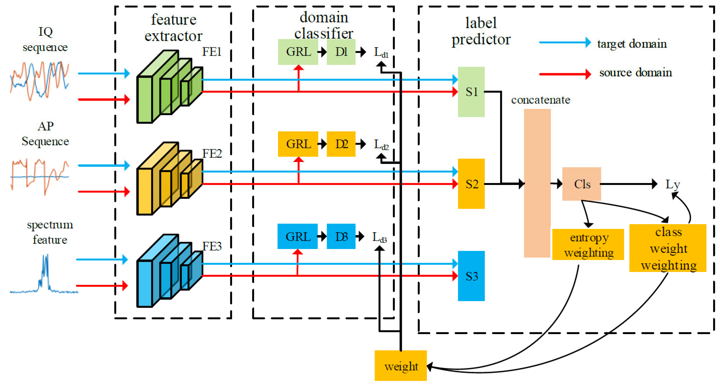
We designed a class weight weighting and entropy weighting mechanism to improve the weight of shared class data samples and effectively address the PDA problem, particularly in scenarios where the number of modulation signal classes in the target domain is smaller than that in the source domain.

(4)

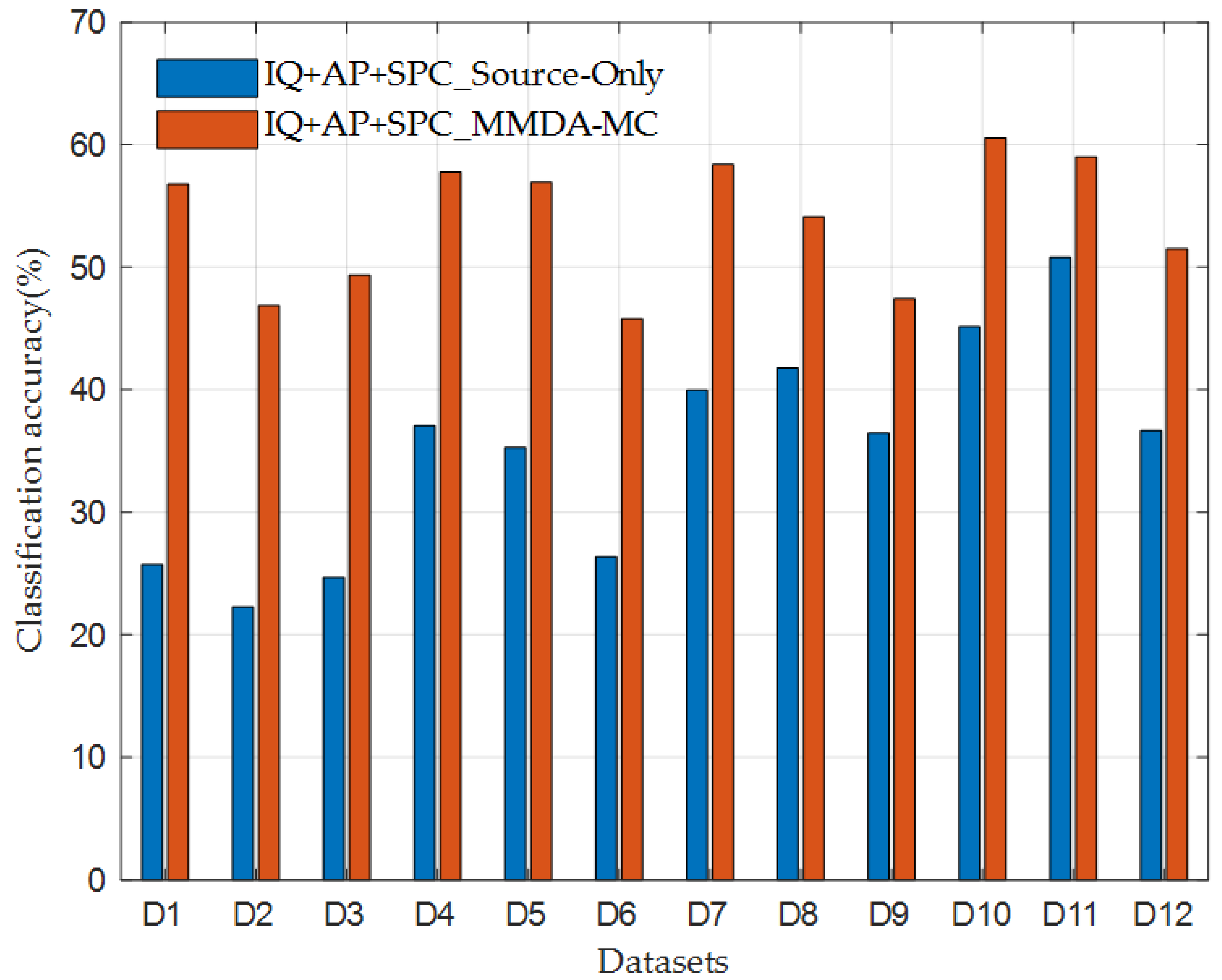
We conducted extensive experiments on two datasets explicitly designed to validate the effectiveness of our approach. The results demonstrated that our method achieves higher classification accuracy in different DA tasks compared with the baseline methods.

The remainder of this study is organized as follows. Section 2 introduces the system model, including the cross-domain learning model, cross-domain AMC model, and calculation computation of multi-modal feature inputs. Section 3 details the proposed classification approach, including multimodal information fusion, architecture, and training steps. Section 4 presents the experimental results and their detailed analysis. Finally, Section 5 concludes this study. The list of abbreviations and notations used in the article are presented in

Table 1. Summary of abbreviations.

Abbreviations	Notations
AMC	Automatic Modulation Classification
DL	Deep Learning
SNR	Signal-to-Noise Ratio
CNN	Convolutional Neural Network
RNN	Recurrent Neural Network
HOCs	Higher-order Cumulants
IQ	In-phase and Quadrature
AP	Amplitude and Phase
NPDA	Non-partial Domain Adaptation
PDA	Partial Domain Adaptation
DA	Domain Adaptation
TL	Transfer Learning
DANN	Domain Adversarial Neural Network
GRL	Gradient Reversal Layer
GANs	Generative Adversarial Network
FE1, FE2, FE3	Feature Extractor
D1, D2, D3	Domain Classifier
Cls	Class Label Predictor
S1, S2, S3	Label Predictor
fc	Fully Connected layer
sps	Samples Per Symbol

and

Table 2. Definition of notation.

Notation	Definition	Notation	Definition
$D$	Domain	$p$,$q$	Marginal probability distribution of domain
$\chi$	Feature space	$n_s$	Number of source domain samples
$X$	Domain samples	$n_t$	Number of target domain samples
$x_i$	i-th feature vector in $X$	$p{c}_t$	Marginal probability distribution of shared classes in the source domain
$T$	Task	$\lambda$	Weight coefficient
$\gamma$	Label space	$L_y$	Cross-entropy loss function of label predictor
$f(•)$	Predictive function	$L_d$	Cross-entropy loss function of domain classifier
$Y$	Labels of domain samples	${\widehat{\theta }}_f$	Saddle point of ${\theta }_f$
$y_i$	i-th label in $Y$	${\widehat{\theta }}_y$	Saddle point of ${\theta }_y$
$P(Y|X)$	Conditional probability distributions of domain	${\widehat{\theta }}_d$	Saddle point of ${\theta }_d$
$D_S$	Source domain	$u$	Learning rate
$T_S$	Source task	$\Re (\mathrm{x})$	Pseudo-function
$D_T$	Target domain	${\rm I}$	Identity matrix
$T_T$	Target task	$\tilde{x}(n)$	Baseband complex signal
$P_S(X)$	Marginal probability distributions of $D_S$	$I(n)$	In-phase component of signal
$P_T(Y)$	Marginal probability distributions of $D_T$	$Q(n)$	Quadrature component of signal
$P(Y_S|X_S)$	Conditional probability distributions of $D_S$	$X_1(k)$	Spectral amplitude
$P(Y_T|X_T)$	Conditional probability distributions of $D_T$	$X_2(k)$	Square spectrum
$G_f$	Feature extractor	$amp(n)$	Normalized instantaneous amplitude
$G_y$	Label predictor	$phase(n)$	Instantaneous phase
$G_d$	Domain classifier	${\widehat{y}}_i$	Predicted label
${\theta }_f$	Parameters of feature extractor	$\eta$	Weight of different classes in the source domain label space
${\theta }_y$	Parameters of label predictor	$w(x)$	Entropy weighting
${\theta }_d$	Parameters of domain classifier	${\eta }_{y_i^s}$	Weight of each source domain sample
$x_i^s$	A single source domain modulated signal sample	$w(x^s)$	Entropy weight vector of source domain sample
$y_i^s$	Label of source domain signal	$w(x^t)$	Entropy weight vector of target domain sample
$x_i^t$	A single target-domain-modulated signal sample without a label	$N$	Batch size
$d_j^{s,t}$	Domain label	$P_C$	Classification accuracy
$C_s$	Label space of source domain	$r$	Current iteration number
$C_t$	Label space of target domain	$M_P$	Number of correctly classified samples
$C_s\backslash C_t$	Outlier classes	$M$	Total number of samples

, respectively.

2. System Model

We will first introduce the cross-domain learning model, then define the cross-domain AMC problem, and finally describe the computation method of multi-feature input adopted in this study.

2.1. Cross-Domain Learning Model

The research methodology employed in this study to resolve the cross-domain AMC problem is based on transfer learning principles. Particularly, we adopt the DANN to align the training and testing data domains.

2.1.1. Transfer Learning

The major task of TL is to transfer learned knowledge from the source to the target domain to improve the learning process of the target task [25]. Thus, we first define “domain” and “task”. A domain $D$ comprises a feature space $\chi$ and marginal probability distribution $P(X)$ in which $X=\{x_1,\dots ,x_n\}$ where $x_i$ is the $i$-th feature vectors in $X$. Hence, $D=\{\chi ,P(X)\}$. A task T in $D$ comprises a label space $\gamma$ and a predictive function $f(•)$ in which $Y=\{y_1,\dots ,y_n\}\in \gamma$, where $y_i$ is the $i$-th label in $Y$. The predictive (or decision) function is learned from the feature vector and label pairs $\{x_i,y_i\}$. Additionally, the predictive function represents the prediction of the corresponding label $f(x_i)$ given instance $x_i$. In this case, the predictive function can be defined as $f(x_i)=P(Y|X)$. Hence, $T=\{\gamma ,f(•)\}$.

Now, we can formally define TL as follows. Given a source domain $D_S$ with a corresponding source task $T_S$, and a target domain $D_T$ with a corresponding source task $T_T$, TL aims to learn the target predictive function $f(•)$ by leveraging the knowledge gained from $D_S$ and $T_S$, where $D_S\ne D_T$ or $T_S\ne T_T$. Note that $D_S\ne D_T$ implies that ${\chi }_S\ne {\chi }_T$ and/or $P_S(X)\ne P_T(Y)$. When ${\chi }_S\ne {\chi }_T$, the feature space of the source and target domains differ. Similarly, $P_S(X)\ne P_T(Y)$ when the marginal distributions of the source and target domain differ. Another scenario of TL is $T_S\ne T_T$, where ${\gamma }_S\ne {\gamma }_T$ and/or $P(Y_S|X_S)\ne P(Y_T|X_T)$. When ${\gamma }_S\ne {\gamma }_T$, the label space of the source and target domains are different. When $P(Y_S|X_S)\ne P(Y_T|X_T)$, the conditional probability distributions of the source and target domains are different.

2.1.2. DANN

In this study, we treat the source and target domains as a whole and train a domain classifier to achieve feature alignment between the two domains. The objective of the domain classifier is to ensure that the deep features extracted from the source and target domains are aligned in the same feature space. This addresses the parameter sensitivity issue that can cause deep-learning-based modulation recognition methods to fail.

Our method utilizes DANN to align the distribution of the source and target domains, thus avoiding the manual designing of the distance losses between the source and target domains. During training, the network spontaneously learns what should be aligned between the two domains and to what extent. This approach typically yields improved results.

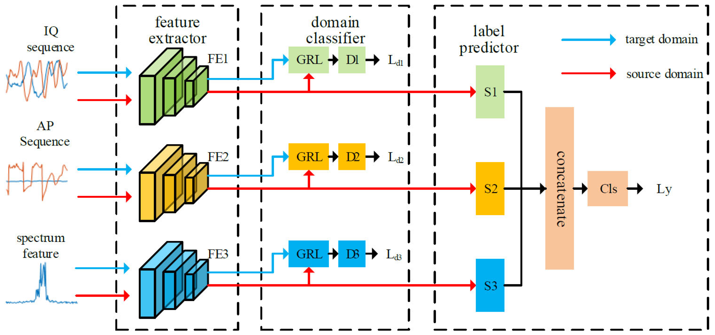
DANN [25] is a representation learning approach for DA in which the training and test data come from similar but different distributions. The advantage of the DA approaches is the ability to learn a mapping between domains when the target domain data are either fully unlabeled or have few labeled samples. DANN’s architecture consists primarily of a feature extractor, label predictor, and domain classifier (Figure 1). The learning feature is required to be domain-invariant except for discriminativeness. Therefore, the domain classifier is designed to discriminate whether the underlying features is from the source or target domain during training. The gradient reversal layer (GRL) [25] propagates the domain classification loss back to the feature extractor, with the weight of the loss function controlled by a hyperparameter λ. Through gradient reversal, the domain adversarial network maximizes the loss of domain classifier while minimizing the loss of the label predictor.

The loss function consists of the source and domain classification loss. The source domain classification loss is used to ensure that the neural network performs well on the source domain data. The domain classification loss aims to align the data distributions of the source and target domains so that the neural network trained on the source domain can also exhibit good classification performance on the unlabeled target domain. By jointly optimizing the source and domain classification loss, we can train a neural network with good generalization performance, enabling it to perform effectively in the target domain.

The core idea of this approach is to use the domain classifier to guide the feature extractor in learning feature representations that have discriminative performance for both the source and target domains. By aligning the source and target domain data features, we can resolve the issue of ineffective deep-learning-based modulation recognition methods caused by parameter sensitivity and improve the model’s generalization performance on unlabeled data.

Therefore, DANN must accomplish the following two core tasks during training. The first task is to accurately classify the source domain data to minimize the loss of the label classifier. The second task is to confuse the source and target domain data to maximize the loss of the domain classifier. The objective function of DANN can be represented as follows.

$$E\left({\theta }_f,{\theta }_y,{\theta }_d\right)=\frac{1}{n_s}{\displaystyle \sum _{i=1}^{n_s}{L}_y}\left(G_y\left(G_f\left(x_i^s;{\theta }_f\right);{\theta }_y\right),y_i^s\right)-\lambda \frac{1}{n_s+n_t}{\displaystyle \sum _{j=1}^{n_s+n_t}{L}_d}\left(G_d\left(G_f\left(x_j^{s,t};{\theta }_f\right);{\theta }_d\right),d_j^{s,t}\right),$$

(1)

where $G_f$ is the feature extractor with parameters ${\theta }_f$; $G_y$ is the label predictor in the source domain with parameter ${\theta }_y$; $G_d$ is the domain classifier with parameter ${\theta }_d$; and the number of samples in the source and target domain is denoted as $n_s$ and $n_t$, respectively. Further, $y_i^s$ and $d_j^{s,t}$ are the source domain category label (only the data in the source domain has the category label) and the domain label (both the source and target domain data have the domain label), respectively; $\lambda$ is the weight coefficient; and $L_y$ and $L_d$ represent the cross-entropy loss function obtained by finding the saddle point ${\widehat{\theta }}_f$, ${\widehat{\theta }}_y$, ${\widehat{\theta }}_d$ such that

$$({\widehat{\theta }}_f,{\widehat{\theta }}_y)=\underset{{\theta }_f,{\theta }_y}{\arg \min }E\left({\theta }_f,{\theta }_y,{\widehat{\theta }}_d\right),$$

(2)

$${\widehat{\theta }}_d=\underset{{\theta }_d}{\arg \min }E\left({\widehat{\theta }}_f,{\widehat{\theta }}_y,{\widehat{\theta }}_d\right).$$

(3)

A saddle point can be found as a stationary point of the following gradient updates.

$${\theta }_f\leftarrow {\theta }_f-u\left(\frac{\partial L_y\left(G_y\left(G_f\left(x_i^s;{\theta }_f\right);{\theta }_y\right),y_i^s\right)}{\partial {\theta }_f}-\lambda \frac{\partial L_d\left(G_d\left(G_f\left(x_j^{s,t};{\theta }_f\right);{\theta }_d\right),d_j^{s,t}\right)}{\partial {\theta }_f}\right),$$

(4)

$${\theta }_y\leftarrow {\theta }_y-u\frac{\partial L_y\left(G_y{\left(G_f\left(x_i^s;{\theta }_f\right);{\theta }_y\right)}_z{y}_i^s\right)}{\partial {\theta }_y}$$

(5)

$${\theta }_d\leftarrow {\theta }_d-u\lambda \frac{\partial L_d\left(G_d\left(G_f\left(x_j^{s,t};{\theta }_f\right);{\theta }_d\right),d_j^{s,t}\right)}{\partial {\theta }_d},$$

(6)

where $u$ is the learning rate.

Ref. [25] added GRL to achieve true end-to-end training and avoid the two-stage training process where the generator and discriminator parameters are fixed separately, as in generative adversarial networks (GANs). Mathematically, we can formally treat the GRL as a “pseudo-function” $\Re (\mathrm{x})$ defined by two (incompatible) equations describing its forward and backpropagation behavior:

$$\Re (\mathrm{x})=\mathrm{x} ,$$

(7)

$$\frac{d\Re }{d\mathrm{x}}=-{\rm I},$$

(8)

where $\mathrm{{\rm I}}$ is an identity matrix. It is worth noting that Equations (7) and (8) define a trainable network layer that does not require parameter updates. It can be easily implemented using existing deep learning tools, specifically by defining the procedures for forward propagation (identity transformation) and backpropagation (multiplication by −1).

Then, we can define the objective “pseudo-function” of $\left({\theta }_f,{\theta }_y,{\theta }_d\right)$ that is being optimized by the stochastic gradient descent as follows:

$$E\left({\theta }_f,{\theta }_y,{\theta }_d\right)=\frac{1}{n_s}{\displaystyle \sum _{i=1}^{n_s}{L}_y}\left(G_y\left(G_f\left(x_i^s;{\theta }_f\right);{\theta }_y\right),y_i^s\right)+\lambda \frac{1}{n_s+n_t}{\displaystyle \sum _{j=1}^{n_s+n_t}{L}_d}\left(G_d\left(G_f\left(x_j^{s,t};{\theta }_f\right);{\theta }_d\right),d_j^{s,t}\right).$$

(9)

2.2. Cross-Domain AMC

The cross-domain AMC problem based on unsupervised DA comprises the source domain $D_s={\left\{\left(x_i^s,y_i^s\right)\right\}}_{i=1}^{n_s}$ with $n_s$ labeled samples and target domain $D_t={\left\{\left(x_i^t\right)\right\}}_{i=1}^{n_t}$ with $n_t$ unlabeled samples. Here, $x_i^s$ represents a single source-domain-modulated signal sample, with a corresponding label $y_i^s$; and $x_i^t$ represents a single-target domain-modulated signal sample without a label. Let us assume that the label space of the source domain contains $\left|C_s\right|$ types of radio signal and is denoted as $C_s$. Similarly, the label space of the target domain contains $\left|C_t\right|$ types of radio signal and is denoted as $C_t$.

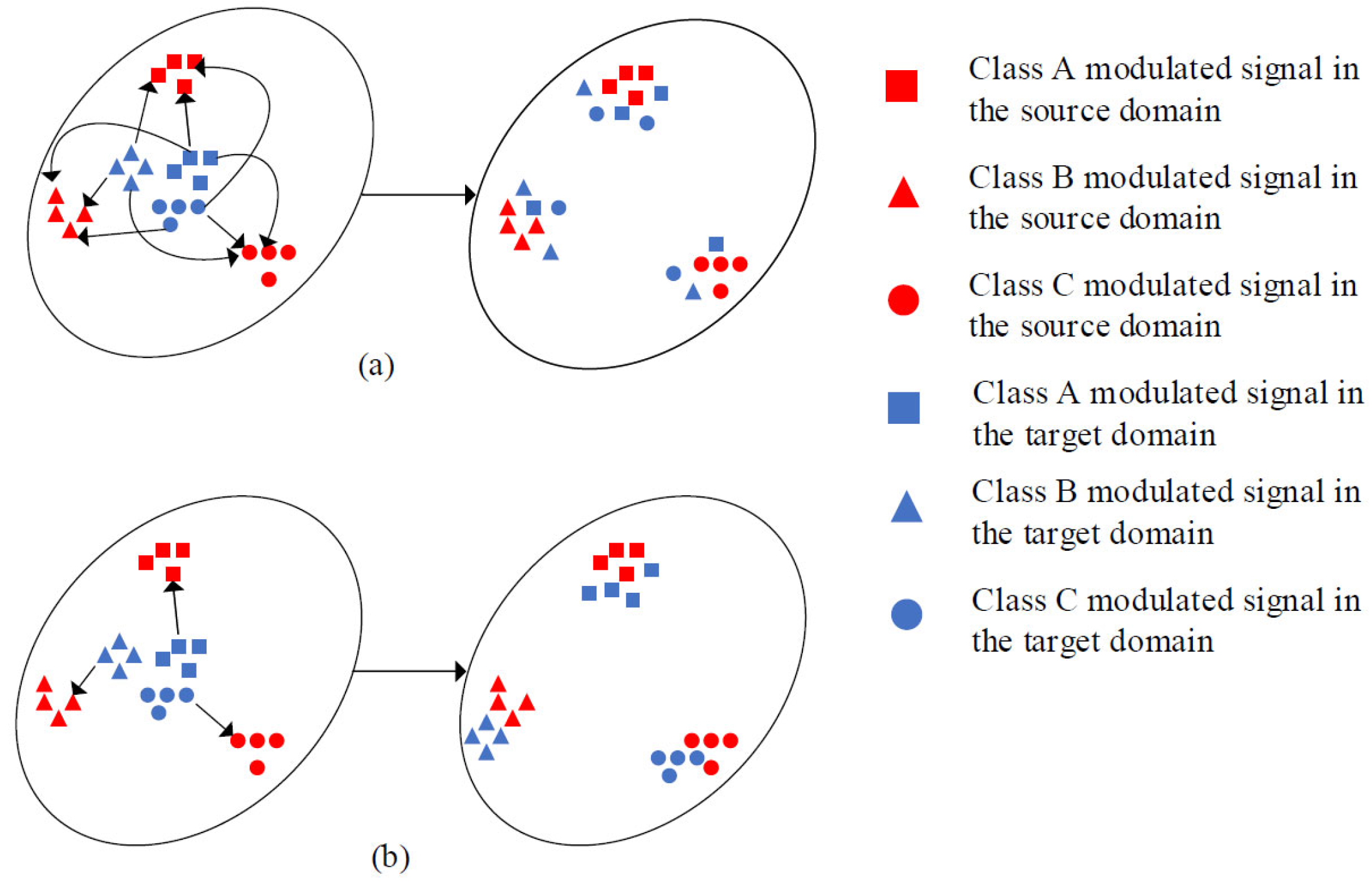
2.2.1. Unsupervised NPDA Problem

For the problem of unsupervised NPDA, we assume that the source and target domains have the same number of labels and label types for radio signals, thus indicating that the domains have the same label space. Let $p$ and $q$ denote the marginal probability distribution of the two domains, where $p\ne q$. The primary objective is to transfer knowledge from the source to the target domain and align the distribution between the target and source domains. Figure 2 is the schematic of the DL-based AMC method directly applied to the unsupervised NPDA problem of AMC and the expected effect to be achieved using the unsupervised NPDA method.

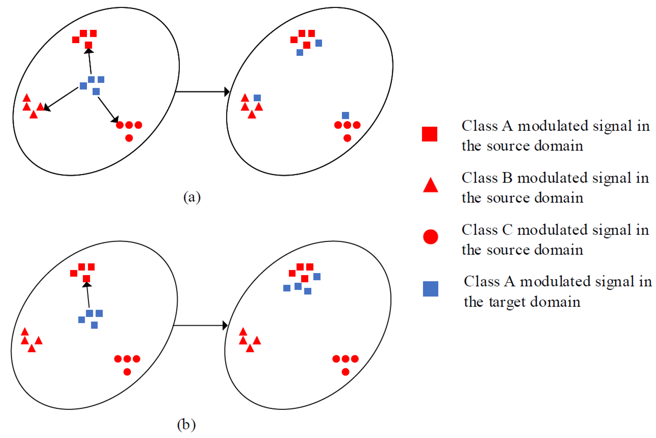
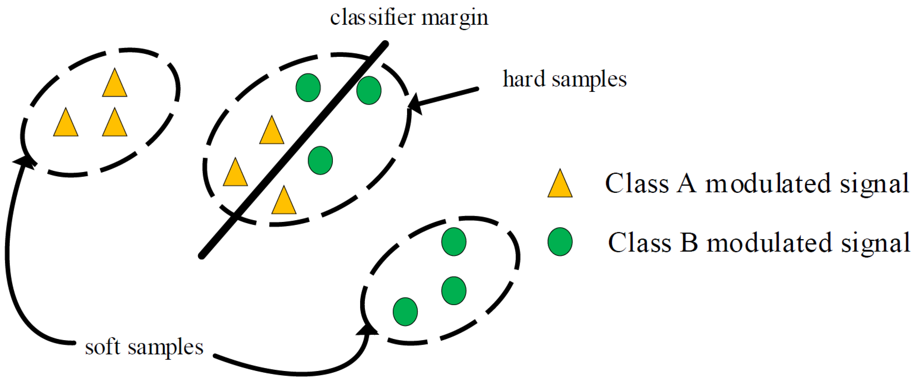
2.2.2. Unsupervised PDA Problem

For unsupervised PDA problem, we assume that the label space of the target domain is a proper subset of the source domain, i.e., $C_s\not\subset C_t$. Here, $p$ and $q$ denote the marginal probability distribution of the two domains, where $p\ne q$, and $p{c}_t$ denotes the marginal probability distribution of source domain samples with labels shared by the two domains, which differs from that of the target domain. The main objective of unsupervised PDA is to align the fine-grained shared label distributions.

In addition to the challenges of different distributions between the source and target domains of the modulated signal and the lack of labels in the target domain, adaptation also involves the difficulty of not knowing the shared label space for the source and target domain modulation signals during training as the label space of target domain $C_t$ is unknown at that time [32]. This poses two technical challenges.

First, directly applying unsupervised NPDA AMC algorithms aligns the global distributions of both domains, thus causing negative transfer due to the existence of outlier classes denoted as $C_s\backslash C_t$ (i.e., signal categories only included in the source domain modulation dataset). Therefore, the matching of outlier classes should be avoided. Second, aligning the distributions of $p{c}_t$ and $q$ to promote positive transfer is goal of this study. Thus, eliminating or reducing the impact of outlier classes in the source domain and promoting the transfer of shared classes (i.e., signal categories included in the source and target domain modulation datasets) from the source domain to the target domain is critical. Figure 3 illustrates this problem, considering a simple case with three modulation signal categories in the source domain and only one in the target domain.

2.3. Multimodal Feature Input Calculation

The AMC method based on image representations (such as eye and constellation diagrams) depends on the accurate estimation of signal modulation parameters; thus, it cannot to classify noncooperative received signals. The length of the sampled data considerably influences the accuracy of estimating higher-order cumulant features is computationally complex.

Therefore, under the noncooperative reception condition, we aimed to reduce computational complexity and data volume while fully using the signal’s multimodal features. We used IQ and AP sequences from the signal’s sequential representation and spectral amplitude and squared signal’s spectral amplitude from the feature representation as inputs to the network. Assuming that the baseband complex signal obtained after the received signal is $\tilde{x}(n)$, the detailed calculation methods are as follows.

IQ sequence (I): The in-phase and quadrature components of the signal are the real and imaginary parts of the signal, as follows:

$$I(n)=real(\tilde{x}(n)),$$

(10)

$$Q(n)=imag(\tilde{x}(n)).$$

(11)

The first modality $F_{iq}$ is the imaginary part and real part of the received signal, which is expressed as:

$$F_{iq}=[I(n);Q(n)].$$

(12)

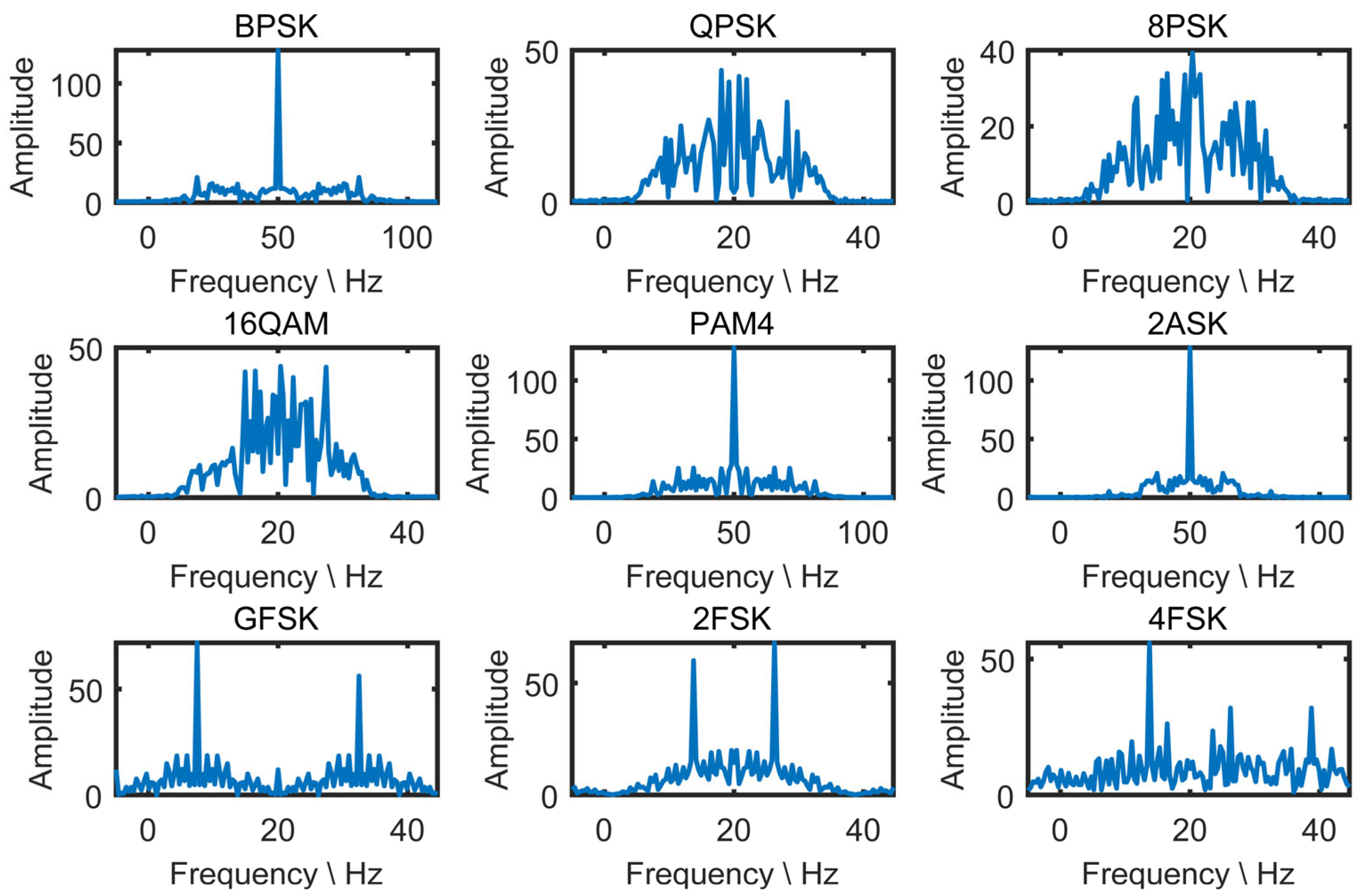
Spectral amplitude and squared signal’s spectral amplitude (S): Calculate the spectral amplitude of the signal, as follows:

$$X_1(k)=\left|{\displaystyle {\sum }_{n=1}^N\tilde{x}(n)e^{-j2\pi kn/N}}\right|,k=0,1,2,\dots ,N-1,$$

(13)

where | • | denotes the modulus operation.

Calculate the squared signal’s spectral amplitude, as follows:

$$X_2(k)=\left|{\displaystyle {\sum }_{n=1}^N{\tilde{x}}^2(n)e^{-j2\pi kn/N}}\right|,k=0,1,2,\dots ,N-1.$$

(14)

The second modality $F_{spc}$ consists of the spectral amplitude and the squared signal’s spectral amplitude, which is expressed as

$$F_{spc}=[X_1(n);X_2(n)],n=1,2,3,\dots N$$

(15)

where $F_{spc},$ represents spectral features of the received signals in the frequency domain for DL models to recognize frequency and phase modulated signals.

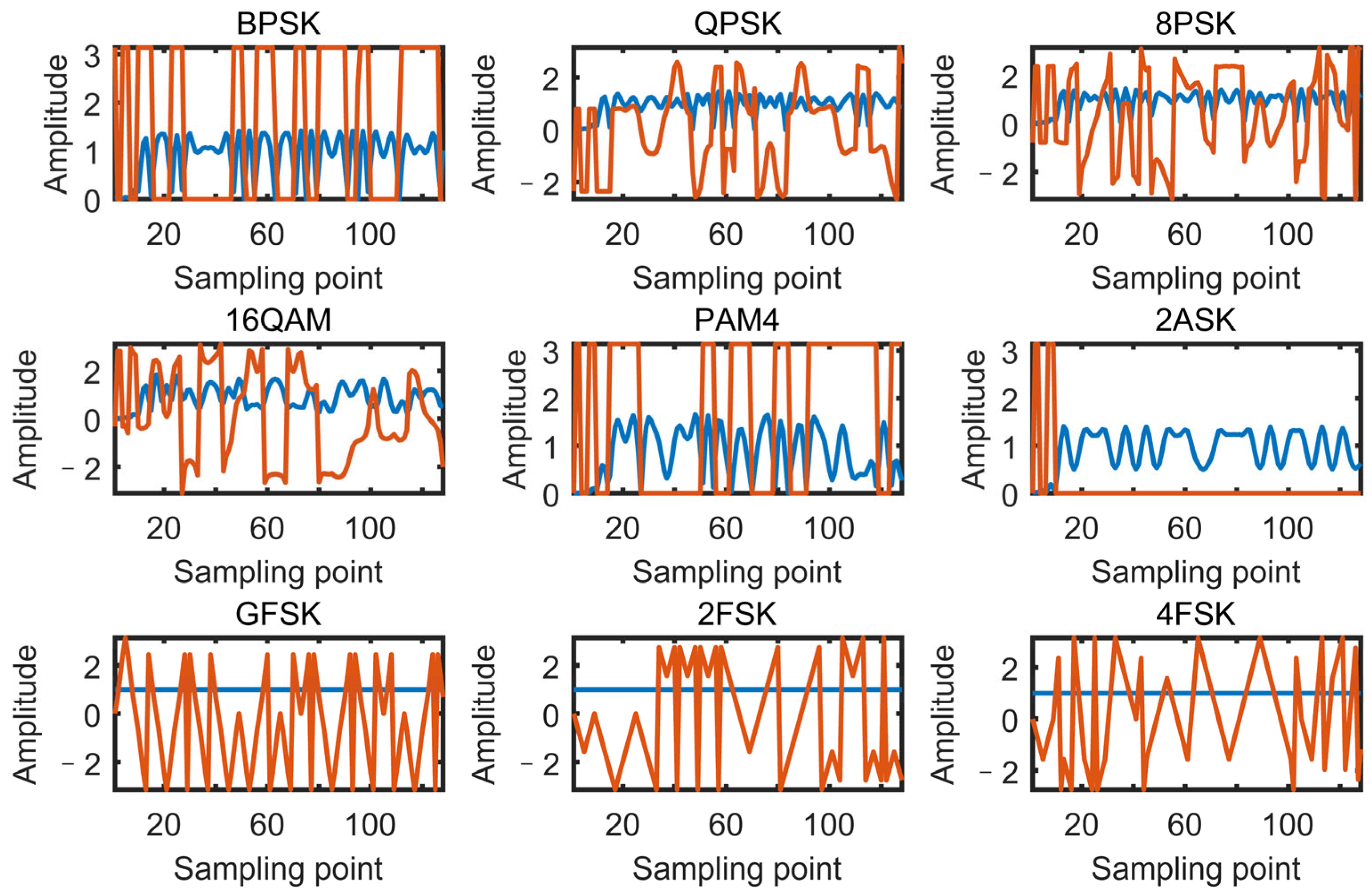
AP sequence (A): Calculate the normalized instantaneous amplitude of the signal, as follows.

$$amp(n)=\frac{\left|\tilde{x}(n)\right|N}{\sqrt{{\displaystyle {\sum }_{n=1}^N{\left|\tilde{x}(n)\right|}^2}}},n=1,2,3,\dots N.$$

(16)

This feature can reflect the amplitude variation of different modulated signals, which is helpful for DL models to recognize amplitude-modulated signals.

Calculate the instantaneous phase of the signal, as follows.

$$phase(n)=\mathrm{atan}2\frac{I(n)}{Q(n)},n=1,2,3,\dots N,$$

(17)

where the value of $phase(n)$ is $(\left.-\pi ,\pi \right]$.

The third modality,$F_{ap}$, comprises instantaneous amplitude and instantaneous frequency, which is expressed as:

$$F_{ap}=[amp(n);phase(n)],n=1,2,3,\dots N.$$

(18)

Figure 4, Figure 5, Figure 6 and Figure 7 present the schematic of features extracted from nine modulation schemes, namely 8PSK, BPSK, 2FSK, 4FSK, 2ASK, GFSK, PAM4, QAM16, and QPSK.

The complementarity between the first and third modalities (IQ and AP) has been proven in previous research [33,34]. It has been shown that (1) algorithms that utilize AP as input data outperform IQ algorithms at high SNR but show opposite results at low SNR; (2) the features extracted from IQ and AP exhibit complementary characteristics.

Furthermore, selecting features with stronger representational power can enhance the performance of existing deep-learning-based AMC. For instance, when ASK has to be distinguished from other signals, choosing instantaneous amplitude features may yield more effective results. Similarly, when differentiating PSK from other signals, selecting instantaneous phase features may be preferred. When the task is to distinguish FSK from other signals, instantaneous frequency features can be a suitable choice. Lastly, constellation mapping can represent a feature of differentiating higher-order modulation schemes.

Therefore, the utilization of modal information should be determined based on the specific signal categories and their corresponding feature selection. The multi-modal feature input that we have chosen here is provided as an example.

3. Proposed Cross-Domain AMC Method Based on Multimodal and TL

3.1. Multimodality DANN Modulation Classification

For the problem of unsupervised NPDA, we proposed the multimodality DANN modulation classification model (MMDA-MC) shown in Figure 8. The network input consists of the multimodal features computed in Section 2.3. FE1, FE2, and FE3 represent the underlying feature extractors and share the same network structure. D1, D2, and D3 are domain classifiers with the same network structure. Cls is the class label predictor. s1, s2, and s3 are the hidden layer outputs of the three feature extractors. The method mainly consists of two key modules: multimodal fusion AMC module and domain adversarial alignment module. We present the training and testing steps of the proposed MMDA-MC in Algorithm 1.

Algorithm 1: Training and Testing Steps of Proposed MMDA-MC

Input: Multimodal features of the source and target domains ${{\{\mathrm{I}}_i^s{,\mathrm{S}}_i^s{,\mathrm{A}}_i^s\}}_{i=1}^{n_s}$,${\left\{{\mathrm{I}}_i^t{,\mathrm{S}}_i^t{,\mathrm{A}}_i^t\right\}}_{i=1}^{n_t}$, the learning rate $u$, and the training epoches $epo$.

Output: Classification accuracy.

1. Initializing the network parameters

Build $G_y$, $G_{f_1}$, $G_{f_2}$, $G_{f_3}$, $G_{d_1}$, $G_{d_2}$, and $G_{d_3}$.

Initialize the ${\theta }_y$, ${\theta }_{f_1}$, ${\theta }_{f_2}$, ${\theta }_{f_3}$, ${\theta }_{d_1}$, ${\theta }_{d_2}$, and ${\theta }_{d_3}$.

2. Training For v = 1, 2, …, $epo$  a. Input ${{\{\mathrm{I}}_i^s{,\mathrm{S}}_i^s{,\mathrm{A}}_i^s\}}_{i=1}^{n_s}$ and ${\left\{{\mathrm{I}}_i^t{,\mathrm{S}}_i^t{,\mathrm{A}}_i^t\right\}}_{i=1}^{n_t}$ into $G_{f_1}$, $G_{f_2}$, and $G_{f_3}$ to extract deep features $G_{f_1}({\mathrm{I}}_i^s;{\theta }_{f_1})$, $G_{f_2}({\mathrm{S}}_i^s;{\theta }_{f_2})$, $G_{f_3}({\mathrm{A}}_i^s;{\theta }_{f_3})$, $G_{f_1}({\mathrm{I}}_i^t;{\theta }_{f_1})$, $G_{f_2}({\mathrm{S}}_i^t;{\theta }_{f_2})$, and $G_{f_3}({\mathrm{A}}_i^t;{\theta }_{f_3})$.  b. Input the deep features into the $G_{f_3}$, $G_{d_1}$, and $G_{d_2}$ to calculate $L_{d_1}$, $L_{d_2}$, and $L_{d_3}$.  c. Concatenate the deep features to obtain fused feature.  d. Input the fused feature into $G_y$ to calculate $L_y$;  e. Add $L_{d_1}$, $L_{d_2}$, $L_{d_3}$, and $L_y$ to obtain $L$.  f. Update ${\theta }_y$, ${\theta }_{f_1}$, ${\theta }_{f_2}$, ${\theta }_{f_3}$, ${\theta }_{d_1}$, ${\theta }_{d_2}$, and ${\theta }_{d_3}$ by using gradient descent.  g. Adjust learning rate $u$.  h. If converges to an extremum or $L$ reaches a preset threshold:  Save weights ${\theta }_y$, ${\theta }_{f_1}$, ${\theta }_{f_2}$, ${\theta }_{f_3}$, ${\theta }_{d_1}$, ${\theta }_{d_2}$, and ${\theta }_{d_3}$.  Stop training.

End

End

3. Testing

Input the concatenated the deep features of the target domain into $G_y$ to calculate the classification accuracy.

It should be noted that a previous study has shown that employing corresponding network structures for different modalities can lead to better feature representations [35]. However, as neural networks become deeper, the performance differences between various network structures may diminish. Therefore, in this work, we concentrate on addressing the challenge of parameter sensitivity, which can impede the effectiveness of deep-learning-based modulation recognition methods, by leveraging multi-modal information and adversarial training. Rather than utilizing multiple network structures to extract deep features from different modal inputs, we have made a deliberate choice to maintain focus and prevent the research from becoming divergent. This decision is reasonable and helps us maintain a concentrated and focused approach to our research.

3.1.1. Multimodal Fusion AMC Module

The source domain label classification loss is calculated by propagating the loss through backpropagation to each feature extractor after fusing and concatenating the deep features extracted from the input multimodal features (I, S, A). Therefore, the source domain label classification loss can be expressed as:

$$\frac{1}{n_s}{\displaystyle \sum _{i=1}^{n_s}{L}_y\left((G_y(G_{f_1}(x_i^s;{\theta }_{f_1})+G_{f_2}(x_i^s;{\theta }_{f_2})+G_{f_3}(x_i^s;{\theta }_{f_3});{\theta }_y),y_i^s\right),}$$

(19)

where $G_{f_1}$, $G_{f_2}$, and $G_{f_3}$ are three feature extractor with parameters ${\theta }_{f_1}$, ${\theta }_{f_2}$ and ${\theta }_{f_3}$; $G_y$ is the label predictor with parameter ${\theta }_y$, respectively; $G_d$ is the domain classifier with parameter ${\theta }_d$; $n_s$ is the number of samples in the source domain; $y_i^s$ is the source domain category label; and $L_y$ represents the cross-entropy loss function.

3.1.2. Domain Adversarial Alignment Module

To leverage the complementary benefits of multimodal information, a domain classifier is applied to each mono-modality feature to align the feature distributions between the source and target domains. Thus, the overall domain classification loss can be defined as:

$$\begin{array}{l}{\lambda }_1\frac{1}{n_s+n_t}{\displaystyle \sum _{j=1}^{n_s+n_t}{L}_{d_1}}\left(G_{d_1}\left(G_{f_1}\left(x_j^{s,t};{\theta }_{f_1}\right);{\theta }_{d_1}\right),d_j^{s,t}\right)\\ +{\lambda }_2\frac{1}{n_s+n_t}{\displaystyle \sum _{j=1}^{n_s+n_t}{L}_{d_2}}\left(G_{d_2}\left(G_{f_2}\left(x_j^{s,t};{\theta }_{f_2}\right);{\theta }_{d_2}\right),d_j^{s,t}\right)\\ +{\lambda }_3\frac{1}{n_s+n_t}{\displaystyle \sum _{j=1}^{n_s+n_t}{L}_{d_3}}\left(G_{d_3}\left(G_{f_3}\left(x_j^{s,t};{\theta }_{f_3}\right);{\theta }_{d_3}\right),d_j^{s,t}\right)\end{array},$$

(20)

where $G_{d_1}$, $G_{d_2}$, and $G_{d_3}$ are three domain classifiers with parameters ${\theta }_{d_1}$, ${\theta }_{d_2}$, and ${\theta }_{d_3}$, respectively; ${\lambda }_1$, ${\lambda }_2$, and ${\lambda }_3$ are the weight coefficients; $d_j^{s,t}$ is the source domain label; and $L_{d_1}$, $L_{d_2}$, and $L_{d_3}$ represent the cross-entropy loss function. Thus, the total loss function can be defined as

$$\begin{array}{l}L=\frac{1}{n_s}{\displaystyle \sum _{i=1}^{n_s}{L}_y\left((G_y(G_{f_1}(x_i^s;{\theta }_{f_1})+G_{f_2}(x_i^s;{\theta }_{f_2})+G_{f_3}(x_i^s;{\theta }_{f_3});{\theta }_y),y_i^s\right)}\\ \hspace{1em}+{\lambda }_1\frac{1}{n_s+n_t}{\displaystyle \sum _{j=1}^{n_s+n_t}{L}_{d_1}}\left(G_{d_1}\left(G_{f_1}\left(x_j^{s,t};{\theta }_{f_1}\right);{\theta }_{d_1}\right),d_j^{s,t}\right)\\ \hspace{1em}+{\lambda }_2\frac{1}{n_s+n_t}{\displaystyle \sum _{j=1}^{n_s+n_t}{L}_{d_2}}\left(G_{d_2}\left(G_{f_2}\left(x_j^{s,t};{\theta }_{f_2}\right);{\theta }_{d_2}\right),d_j^{s,t}\right)\\ \hspace{1em}+{\lambda }_3\frac{1}{n_s+n_t}{\displaystyle \sum _{j=1}^{n_s+n_t}{L}_{d_3}}\left(G_{d_3}\left(G_{f_3}\left(x_j^{s,t};{\theta }_{f_3}\right);{\theta }_{d_3}\right),d_j^{s,t}\right)\end{array}.$$

(21)

The loss function of the label classifier applies only to the source domain, whereas the loss function of the domain classifier applies to both the source and target domains.

3.2. Class-Entropy Weighted Multimodality DANN Modulation Classification

Directly applying DANN to unsupervised PDA AMC problems can degrade performance owing to negative transfer caused by outlier classes, which can be reduced by mitigating the influence of outlier classes [32]. Therefore, the main ideas in [32,36,37,38,39] include assigning higher class weights to shared class samples and lower weights to outlier class samples from the source domain, either in the label predictor or the domain adversarial classifier. Our approach identifies the modulation schemes of the target domain. It assigns higher weights to source domain samples that belong to the same class as the target domain by introducing a class weight weighting and entropy weighting mechanism into the proposed early MMDA-MC model. The modified model is named WMMDA-MC.

The output of the label predictor ${\widehat{y}}_i=G_y(x_i)$ presents a probability distribution in the source domain label space $C_S$ for each input sample $x_i$. This distribution effectively describes the likelihood of a sample belonging to a certain class. As the label spaces of outlier classes and shared classes do not overlap, the label predictor should assign a sufficiently low probability of predicting an outlier class for shared class samples in the target domain. Based on the output of the label predictor for target domain samples, we can determine the weights of each class in the target domain and share these weights with the source domain samples. The impact of prediction errors can be reduced by averaging the SoftMax predictions of all target domain samples. Ultimately, the contribution of each class in the source domain to training can be represented as

$$\eta =\frac{1}{n_t}{\displaystyle \sum _{i=1}^{n_t}{\widehat{y}}_i},$$

(22)

where $\eta$ is a $\left|C_S\right|,$-dimensional vector that quantitatively describes the different categories in the source domain label space during training. Considering that this vector is obtained from the output of the target domain samples in the label predictor and that the target domain does not include outlier classes, the weights assigned to the outlier classes in $\eta$ should be noticeably smaller than those assigned to the shared classes.

In addition to reducing negative transfer, promoting positive transfer from $p{c}_t$ to $q$ is also important. Multimodal information in the signal can enhance the confidence of the label predictor’s predictions, thus enabling more accurate assignment of appropriate weights to the shared and outlier classes. Furthermore, DANN can better facilitate the transfer between the shared classes in the source and target domains.

According to [39,40], for PDA problems, having every sample from the source and target domains equally participate in domain adversarial training is unreasonable. The presence of difficult samples to accurately predict and located near the label predictor can negatively impact domain adversarial training. These difficult-to-predict samples are referred to as “hard samples”, whereas easily predictable samples are called “soft samples”. Figure 9 illustrates soft and hard samples in the simplest binary classification case. The existence of hard samples affects the transfer ability of soft samples; hence, the weight of hard samples in domain adversarial training must be reduced, whereas that of the soft samples must be increased. Hard samples primarily originate from two sources. As outlier and shared classes are orthogonal, no outlier classes exist in the target domain. Therefore, outlier classes are comparatively harder to transfer and lack directionality, resulting in more difficulty in accurate prediction. Moreover, hard-to-transfer samples within the shared classes are fewer, and they can be measured using the conditional entropy criterion defined as

$$H(G_y(x_i))=-{\displaystyle {\sum }_{k=1}^{\left|C_S\right|}{y}_i^k\log (}{y}_i^k).$$

(23)

According to the optimization principle in [40], in adversarial training, entropy weighting is applied to each sample and expressed as

$$w(x)=1+e^{-H(G_y(x_i))}.$$

(24)

The total loss function for the PDA problem is modified by incorporating Equations (22)–(24) into Equation (21), as follows.

$$\begin{array}{l}L=\frac{1}{n_s}{\displaystyle \sum _{i=1}^{n_s}{\eta }_{y_i^s}{L}_y\left((G_y(G_{f_1}(x_i^s;{\theta }_{f_1})+G_{f_2}(x_i^s;{\theta }_{f_2})+G_{f_3}(x_i^s;{\theta }_{f_3});{\theta }_y),y_i^s\right)}\\ {{\displaystyle }}^{}+{\displaystyle \sum _{k=1}^3{\lambda }_k}\frac{1}{n_s}{\displaystyle \sum _{i=1}^{n_s}w(x_i^s){\eta }_{y_i^s}{L}_{d_k}}\left(G_{d_k}\left(G_{f_k}\left(x_i^s;{\theta }_{f_k}\right);{\theta }_{d_k}\right),d_i^s\right)\\ {{\displaystyle }}^{}+{\displaystyle \sum _{k=1}^3{\lambda }_k}\frac{1}{n_t}{\displaystyle \sum _{j=1}^{n_t}w(x_j^t)L_{d_k}}\left(G_{d_k}\left(G_{f_k}\left(x_j^t;{\theta }_{f_k}\right);{\theta }_{d_k}\right),d_j^t\right)\end{array},$$

(25)

where ${\eta }_{y_i^s}$ represents the weight of each source domain sample, obtained by taking the $y_i^s$-th value in the vector.

The proposed WMMDA-MC method modified according to the loss function is shown in Figure 10. We present the training and testing steps of the proposed MMDA-MC in Algorithm 2.

Algorithm 2: The Training and Testing Steps of Proposed WMMDA-MC

Input: the multimodal features of the source and target domains ${{\{\mathrm{I}}_i^s{,\mathrm{S}}_i^s{,\mathrm{A}}_i^s\}}_{i=1}^{n_s}$,${\left\{{\mathrm{I}}_i^t{,\mathrm{S}}_i^t{,\mathrm{A}}_i^t\right\}}_{i=1}^{n_t}$, the learning rate $u$, and the number of iterations $iter$.

Output: Classification accuracy.

1. Initializing the network parameters

Build $G_y$, $G_{f_1}$, $G_{f_2}$, $G_{f_3}$, $G_{d_1}$, $G_{d_2}$, and $G_{d_3}$.

Initialize the ${\theta }_y$, ${\theta }_{f_1}$, ${\theta }_{f_2}$, ${\theta }_{f_3}$, ${\theta }_{d_1}$, ${\theta }_{d_2}$, and ${\theta }_{d_3}$.

2. Training For v = 1, 2, …, $iter$  a. If $iter\ne 1$ and is a multiple of the test interval Input ${\left\{{\mathrm{I}}_i^t{,\mathrm{S}}_i^t{,\mathrm{A}}_i^t\right\}}_{i=1}^{n_t}$ into $G_{f_1}$, $G_{f_2}$, and $G_{f_3}$ to extract deep features $G_{f_1}({\mathrm{I}}_i^t;{\theta }_{f_1})$, $G_{f_2}({\mathrm{S}}_i^t;{\theta }_{f_2})$, and $G_{f_3}({\mathrm{A}}_i^t;{\theta }_{f_3})$. Concatenate these deep features and input them to $G_y$ to get SoftMax output (target_softmax). Take the average of target_softmax to obtain the class weight vector $\eta$. If $\eta$ exists     Update $\eta$ End End  b. Input ${{\{\mathrm{I}}_i^s{,\mathrm{S}}_i^s{,\mathrm{A}}_i^s\}}_{i=1}^{n_s}$ and ${\left\{{\mathrm{I}}_i^t{,\mathrm{S}}_i^t{,\mathrm{A}}_i^t\right\}}_{i=1}^{n_t}$ into $G_{f_1}$, $G_{f_2}$, and $G_{f_3}$ to extract deep features $G_{f_1}({\mathrm{I}}_i^s;{\theta }_{f_1})$, $G_{f_2}({\mathrm{S}}_i^s;{\theta }_{f_2})$, $G_{f_3}({\mathrm{A}}_i^s;{\theta }_{f_3})$, $G_{f_1}({\mathrm{I}}_i^t;{\theta }_{f_1})$, $G_{f_2}({\mathrm{S}}_i^t;{\theta }_{f_2})$, and $G_{f_3}({\mathrm{A}}_i^t;{\theta }_{f_3})$.  c. Concatenate $G_{f_1}({\mathrm{I}}_i^s;{\theta }_{f_1})$, $G_{f_2}({\mathrm{S}}_i^s;{\theta }_{f_2})$, and $G_{f_3}({\mathrm{A}}_i^s;{\theta }_{f_3})$ into $G_y$ to get SoftMax output (source_softmax).  d. Calculate the source domain sample entropy weight vector $w(x^s)$ based on source_softmax.  e. If $\eta$ exists Apply class weight weighting to each source domain sample’s cross-entropy loss to obtain the weighted source domain label classification losses. End  f. Concatenate $G_{f_1}({\mathrm{I}}_i^t;{\theta }_{f_1})$, $G_{f_2}({\mathrm{S}}_i^t;{\theta }_{f_2})$, and $G_{f_3}({\mathrm{A}}_i^t;{\theta }_{f_3})$ into $G_y$ to get SoftMax output (target_softmax).  g. Calculate the source domain sample entropy weight vector $w(x^t)$ based on target_softmax.  h. Input the deep features into the $G_{d_1}$, $G_{d_2}$, and $G_{d_3}$ to calculate $L_{d_1}$, $L_{d_2}$, and $L_{d_3}$. The cross-entropy losses for each source and target domain sample should be weighted using the respective entropy weights $w(x^s)$ and class weights $w(x^t)$  i. Input the fused source domain feature into $G_y$ to calculate $L_y$.  j. Add $L_{d_1}$, $L_{d_2}$, $L_{d_3}$, and $L_y$ to obtain $L$.  k. Update ${\theta }_y$, ${\theta }_{f_1}$, ${\theta }_{f_2}$, ${\theta }_{f_3}$, ${\theta }_{d_1}$, ${\theta }_{d_2}$, and ${\theta }_{d_3}$ by using gradient descent.  l. Adjust learning rate $u$.  m. If converges to an extremum or $L$ reaches a preset threshold:    Save weights ${\theta }_y$, ${\theta }_{f_1}$, ${\theta }_{f_2}$, ${\theta }_{f_3}$, ${\theta }_{d_1}$, ${\theta }_{d_2}$, and ${\theta }_{d_3}$.    Stop training.  End   End

3. Testing

Input the concatenated the deep features of the target domain into $G_y$ to calculate the classification accuracy.

4. Numerical Results and Performance Analysis

4.1. Implementation Details

4.1.1. Model Network Structure

The feature extractor used in this study mainly consists of five convolutional layers (conv1, conv2, conv3, conv4, and conv5) and a fully connected layer (fc1) for extracting features from the source and target domains. ReLU is used as the activation function, and BatchNorm is applied for normalization. Additionally, pooling layers are added after conv2, conv3, conv4, and conv5 to reduce data dimensionality. The original input size of the feature extractor is N × 2 × 128, and it is reshaped using the Reshape function before being fed into the feature extractor as N × 1 × 2 × 128, where N represents the batch size. An AdaptiveAvgPool2d layer conducts binary adaptive mean aggregation, thus ensuring that the features extracted by each feature extractor have consistent dimensions during fusion.

The label predictor consists of two fully connected layers (fc1, fc2) for predicting the labels of the source domain data. ReLU is the activation function. The hidden layer features outputted by the feature extractor are fused and concatenated before being input to the label prediction classifier.

The domain classifier includes three fully connected layers (fc1, fc2, and fc3) for discriminating whether the hidden layer output from the feature extractor belongs to the source or target domains. ReLU is used as the activation function, and each domain classifier is preceded by a GRL.

The Adam optimizer is used for optimizing the feature extractor, label predictor, and domain classifier. A restarted cosine annealing method [41] is applied to update the learning rate at the end of each epoch. The network layouts for each module are presented in

Table 3. CNN architecture layout of feature extractor.

Layers	Output Shape
Reshape	$N\times 1\times 2\times 128$
Conv (filter 32, size = (2,7), stride = 2, padding = (0,3), bias = True)	$N\times 32\times 1\times 64$
BatchNorm2d (32) + ReLU	$N\times 32\times 1\times 64$
Conv (filter 64, size = (1,3), stride = 1, padding = (0,1), bias = True)	$N\times 64\times 1\times 64$
BatchNorm2d (64) + ReLU	$N\times 64\times 1\times 64$
MaxPool2d (size = (1,2))	$N\times 64\times 1\times 32$
Conv (filter 128, size = (1,3), stride = 1, padding = (0,1), bias = True)	$N\times 128\times 1\times 32$
BatchNorm2d (128) + ReLU	$N\times 128\times 1\times 32$
MaxPool2d (size = (1,2))	$N\times 128\times 1\times 16$
Conv (filter 256, size = (1,3), stride = 1, padding = (0,1), bias = True	$N\times 256\times 1\times 16$
BatchNorm2d (256) + ReLU	$N\times 256\times 1\times 16$
MaxPool2d (size = (1,2))	$N\times 512\times 1\times 8$
Conv (filter 512, size = (1,3), stride = 1, padding = (0,1), bias = True)	$N\times 512\times 1\times 8$
BatchNorm2d (512) + ReLU	$N\times 512\times 1\times 8$
MaxPool2d (size = (1,2))	$N\times 512\times 1\times 4$
AdaptiveAvgPool2d ((1,1))	$N\times 512\times 1\times 1$
Flatten	$N\times 512$
Dense (512,128)	$N\times 128$
BatchNorm1d (128) + ReLU + Dropout	$N\times 128$

,

Table 4. CNN architecture layout of label predictor.

Layers	Output Shape
Dense (384,192)	$N\times 192$
ReLU + Dropout	$N\times 192$
Dense (192,192)	$N\times 192$
ReLU + Dropout	$N\times 192$
Dense (192,9)	$N\times 9$

and

Table 5. CNN architecture layout of domain classifier.

Layers	Output Shape
Dense (128,128)	$N\times 128$
ReLU + Dropout	$N\times 128$
Dense (128,128)	$N\times 128$
ReLU + Dropout	$N\times 128$
Dense (128,2)	$N\times 2$

.

4.1.2. Simulation Environment and Evaluation Metric

The DL environment is configured with Python 3.8.0, pytorch 1.6.0, cuda10.2.89 on Windows Server 2012 R2 Standard. The CPU is dual Intel(R) Xeon(R) Gold 6230R, with NVIDIA Tesla V100 and 128 GB memory.

For the MMDA-MC method experiment, the optimizer batch size is set to 5000; the epoch is 50, and ${\lambda }_i$, i = 1, 2, 3; all three parameters remain the same. As the epochs iterate from 0 to 1, the strategy used in [42] is adopted to update ${\lambda }_i$ such that ${\lambda }_i=\frac{2}{1+e^{-10r}}-1$, where $r$ represents the current iteration number divided by the total iteration number. In the early stage of training, ${\lambda }_i$ tends to be 0, thus indicating the importance of optimizing the label predictor. In the later training stages, ${\lambda }_i$ tends to be 1, thus indicating equal importance in optimizing the label predictor and domain classifier. The AMC performance metric is defined as classification accuracy:

$$P_C=\frac{M_P}{M},$$

(26)

where $M_P$ represents the number of correctly classified samples and $M$ represents the total number of samples.

For the WMMDA-MC method experiment, the optimizer batch size is set to 400, iterations are set to 40,000 (as the sample sizes of the source and target domains are different, epoch is not used for counting iterations), test interval is set to 40,000, and the initial learning rate is set to 1 × 10⁻³.

4.2. Dataset Generation

The datasets were created following the method described in [31], which includes five parts: symbol data generation, digital modulation, channel modeling, normalization, and storage.

Based on the unsupervised NPDA problem for AMC mentioned in Section 2.2.2, we designed a typical cross-domain dataset with different parameters and reception conditions to verify the good classification performance and generalization ability of the MMDA-MC method, named Dataset A. By adjusting the SNR, channel types, and samples per symbol (sps), we controlled different domains of data. Dataset A is divided into 12 subsets, named $D_n$, $n=1,2,\dots n$, containing 8PSK, BPSK, 2FSK, 4FSK, 2ASK, GFSK, PAM4, QAM16, and QPSK, which are nine typical digital modulation schemes. The number of sampling points for each signal sample was 128. Each subset contains 1200 training samples, 400 validating samples and 400 testing samples for each modulation scheme at different SNRs. The parameter settings are presented in

Table 6. Unsupervised NPDA datasets parameter settings.

Dataset	SNR	Channel	sps
$D_1$	[20, 30] dB, interval: 2	AWGN	8
$D_2$	[20, 30] dB, interval: 2	AWGN	4
$D_3$	[20, 30] dB, interval: 2	AWGN	16
$D_4$	[20, 30] dB, interval: 2	Rician	8
$D_5$	[20, 30] dB, interval: 2	Rician	4
$D_6$	[20, 30] dB, interval: 2	Rician	16
$D_7$	[−4, 6] dB, interval: 2	AWGN	8
$D_8$	[−4, 6] dB, interval: 2	AWGN	4
$D_9$	[−4, 6] dB, interval: 2	AWGN	16
$D_{10}$	[−4, 6] dB, interval: 2	Rician	8
$D_{11}$	[−4, 6] dB, interval: 2	Rician	4
$D_{12}$	[−4, 6] dB, interval: 2	Rician	16

, and the remaining parameters are kept consistent. Based on the 12 subsets, we designed $12\times 11=132$ DA tasks, denoted as $D_i\to D_j$, $i=1,2,\dots ,12$; $j=1,2,\dots ,12$; $i\ne j$ where the left side of $\to$ represents the labeled source domain dataset and the right side represents the unlabeled target domain dataset.

We introduced two research variables, sps and the number of modulation schemes, to further validate that the modified WMMDA-MC model can effectively address not only unsupervised NPDA but also unsupervised PDA. The parameter sps, when the sampling rate is the same, can control the symbol rate of the modulated signal, which significantly effects transmission rate, bandwidth requirements, and noise resistance in digital communication. Therefore, we specifically selected sps as the experimental variable. Additionally, other source and target domain data parameters were kept consistent to avoid the effects of other interfering variables, except for the difference in sps and modulation scheme types. We designed dataset B, which comprises BPSK, QPSK, 8PSK, PAM4, QAM16, GFSK, CPFSK, and QAM64 modulation schemes, used for AMC under Rician channel conditions.

Table 7. Rician channel parameter settings.

Parameter	Value
sampling rate	200 × 103
sampling rate offset standard deviation	0.01 Hz
maximum sampling rate offset	50 Hz
center frequency offset standard deviation	0.01 Hz
maximum center frequency offset	500 Hz
multipath delay	[0, 0.9, 1.7]
multipath gain	[1, 0.8, 0.3]
SNR	[0, 18] dB, interval: 2

presents the parameter settings for the Rician channel. The SNR ranges from 0 to 18 dB with an interval of 2 dB.

Dataset B includes two subsets. Each subset contains 1200 training samples, 400 validating samples and 400 testing samples for each modulation scheme at different SNRs. The subset with a sps of 8 is named $D_{s8}$ and will be considered the source domain because it contains all eight modulation schemes. The subset with an sps of 4 is further divided into eight datasets based on the included modulation types. For example, the dataset containing only the first modulation type (BPSK) is named $D_{s4\_1}$.

These datasets collectively form the target domain, and the label space of the target domain should be a proper subset of the source domain label space. Here, when $D_{s4\_8}$ is used as the target domain, the PDA problem becomes an NPDA problem. Based on these nine datasets from the source and target domains, we design eight DA tasks for each method, denoted as $D_{s8}\to D_{s4\_i}$, $i=1,2,\dots 8$, where the left side of ”$\to$” represents the labeled source domain dataset and the right side represents the unlabeled target domain dataset.

4.3. Baseline

4.3.1. Supervised Learning

Supervised learning algorithms are used for comparison to explore the upper limit of classification accuracy in DA methods. Currently, most AMC algorithms based on DL are trained on labeled datasets and tested on datasets with the same distribution as the trained datasets. This method is referred to as “supervised” in this study. The network structure of the supervised method is composed by concatenating the feature extractor and label predictor introduced in Section 3.

4.3.2. Supervised Learning with Different Source and Target Domain Distributions

To compare the performance gain of DA methods with current DL-based AMC algorithms in practical scenarios, we designed a “source-only” method. The training was conducted using the supervised network structure, whereas testing was performed on a target domain different from the source domain.

4.4. Effectiveness Analysis of the Multimodal Fusion Strategy

This section verifies the effectiveness of multimodal fusion in DL-based AMC algorithms. It tests the classification performance of the “supervised” method under different input feature combinations on a target domain dataset with the same distribution as the source domain. Figure 11 and

Table 8. Test accuracy for different combinations of input on different dataset (%).

	SPC	IQ	AP	IQ + SPC	IQ + AP	AP + SPC	IQ + SPC + AP
$D_1$	82.53	99.75	99.69	99.77	99.98	99.78	99.98
$D_2$	89.64	99.97	99.81	99.99	100.00	99.89	100.00
$D_3$	86.41	98.25	98.52	98.47	99.60	99.17	99.67
$D_4$	77.59	86.37	85.82	95.19	95.98	94.19	96.94
$D_5$	75.75	85.08	84.50	89.42	91.66	90.08	94.47
$D_6$	83.99	86.34	85.23	93.51	94.96	94.40	96.13
$D_7$	75.90	80.09	76.58	85.11	87.50	86.54	89.25
$D_8$	75.59	77.01	74.34	82.91	83.60	81.43	86.75
$D_9$	74.19	78.56	84.31	83.49	88.51	88.87	90.48
$D_{10}$	69.54	58.38	70.27	73.52	71.94	74.62	75.72
$D_{11}$	62.10	54.19	55.00	68.72	65.46	69.28	71.11
$D_{12}$	70.51	57.12	73.21	73.61	73.50	75.87	77.10
average value	76.98	80.09	82.27	86.98	87.72	87.84	89.80

present the average classification accuracy; the column headers represent different feature combinations fed into the network, and the row headers represent different datasets. Using basic features such as amplitude, phase, and frequency for learning and training can effectively achieve AMC under high SNR Gaussian channels. Furthermore, multimodal fusion outperforms single-feature approaches in classification performance across different channels, SNRs, signal parameters, and other datasets. Moreover, the classification performance increases when more modal features are used as input. This demonstrates that multimodal information can achieve better complementary gains by helping the network learn and understand the input objects, thus improving the network’s classification performance.

4.5. Validity Analysis of Cross-Domain AMC

This section verifies the effectiveness of the MMDA-MC method for solving the unsupervised NPDA problem in cross-domain AMC and analyzes the impact of the channel, SNR, and symbol rate. Multimodal information is employed, with “source-only” serving as the control group.

Table 9. Test accuracy of different algorithms in various datasets (%).

	D1	D2	D3	D4	D5	D6	D7	D8	D9	D10	D11	D12	Average
source-only	25.73	22.26	24.68	37.04	35.26	26.36	39.95	41.77	36.45	45.13	50.78	36.65	35.17
MMDA-MC	56.76	46.86	49.35	57.76	56.94	45.78	58.38	54.09	47.42	60.55	59.00	51.49	53.70
improved	31.03	24.60	24.67	20.72	21.68	19.42	18.43	12.32	10.97	15.42	8.22	14.84	18.53

presents the average classification accuracy, where the column headers indicate the current dataset as the source domain and others as the target domain. For visual comparison, Figure 12 shows a histogram comparing the two methods. Evidently, when the target and source domain data differ, the accuracy of the DL-based AMC method decreases significantly, thus indicating significant challenges in realistic scenarios. However, the proposed MMDA-MC demonstrates clear advantages in such scenarios. Compared with “source-only” without cross-domain training, it improves classification accuracy from 8.22% to 31.03%.

Analyzing the different domain discrepancies caused by varying parameters between the source and target domains is important for evaluating the MMDA-MC method’s performance. For experimental convenience and demonstration, all 132 DA tasks generated from the 12 datasets are divided into seven categories based on the types and combinations of parameter variations.

Table 10. Various cross-domain adaptation tasks.

ID	Name	sps	Channel	SNR
1	DT110	1	1	0
2	DT101	1	0	1
3	DT011	0	1	1
4	DT100	1	0	0
5	DT010	0	1	0
6	DT001	0	0	1
7	DT000	0	0	0

summarizes the DA task mappings: “1” indicates that the parameter remains consistent between the source and target domains, whereas “0” indicates a change. For example, DT110 represents scenarios where the source and target domains have consistent symbol rates and channels but varying SNR.

The results presented in Table 11 indicate the following.

(1)

Overall, the average classification accuracy improvement ranges from 11.50% (DT101) to 20.58% (DT100), thus demonstrating that the MMDA-MC method can enhance classification performance even when there are one or multiple parameter differences between the source and target domains.

(2)

Under single parameter changes: When only the SNR or channel differs (DT110 and DT101, respectively) between the source and target domains, the MMDA-MC method achieves relatively high average classification accuracy of 75.94% and 74.72%, respectively. This indicates that the feature distributions are more similar when only the SNR or channel varies, facilitating feature distribution alignment. However, when only the sps differ (DT011), the average classification accuracy reduces to 58.32%. Particularly, when SNR and channel change simultaneously (DT100), the average classification accuracy is 63.39%, higher than in the case of sps difference alone. This demonstrates that a difference in sps reduces feature similarity, thereby increasing the difficulty in aligning the feature distributions between the source and target domains and significantly impacting classification performance.

(3)

When two or three parameters vary, particularly for DT000, although the MMDA-MC method improves the average classification accuracy compared with the “source-only” method, the accuracy is only 38.10%. Thus, DA methods can enhance classification performance when the differences between the source and target domains are significant. However, the gain in classification performance for the target domain is also limited owing to limited source domain knowledge.

Table 11. Test accuracy of different algorithms in various cross-domain adaptation task (%).

ID	Code Name	Classification Accuracy		Improvement		Number of Tasks
		MMDA-MC	Source-Only	Average	Max	Test	Improved
1	DT110	75.94	54.97	18.65	38.15	12	12
2	DT101	74.72	63.22	11.50	35.10	12	12
3	DT011	58.32	39.61	18.71	52.86	24	24
4	DT100	63.39	42.56	20.83	36.14	12	12
5	DT010	48.32	27.74	20.58	36.73	24	24
6	DT001	43.57	25.06	18.51	46.32	24	24
7	DT000	38.10	19.51	18.59	35.73	24	24

Table 11. Test accuracy of different algorithms in various cross-domain adaptation task (%).

ID	Code Name	Classification Accuracy		Improvement		Number of Tasks
		MMDA-MC	Source-Only	Average	Max	Test	Improved
1	DT110	75.94	54.97	18.65	38.15	12	12
2	DT101	74.72	63.22	11.50	35.10	12	12
3	DT011	58.32	39.61	18.71	52.86	24	24
4	DT100	63.39	42.56	20.83	36.14	12	12
5	DT010	48.32	27.74	20.58	36.73	24	24
6	DT001	43.57	25.06	18.51	46.32	24	24
7	DT000	38.10	19.51	18.59	35.73	24	24

4.6. Validity Analysis of Partial Cross-Domain AMC

This section validates the effectiveness of the WMMDA-MC for solving the unsupervised PDA problem in cross-domain AMC. The compared algorithms include supervised, source-only, and MMDA-MC.

Table 12. Test accuracy of different algorithms in various cross-domain adaptation tasks (%).

	Supervised	WMMDA-MC	MMDA-MC	Source-Only
$D_8\to D_{4\_1}$	100.00	100.00	60.43	70.55
$D_8\to D_{4\_2}$	100.00	98.88	46.79	85.10
$D_8\to D_{4\_3}$	100.00	94.58	63.41	57.76
$D_8\to D_{4\_4}$	100.00	87.92	82.32	68.32
$D_8\to D_{4\_5}$	99.93	99.39	87.10	72.63
$D_8\to D_{4\_6}$	99.09	87.37	80.09	66.63
$D_8\to D_{4\_7}$	89.54	84.49	82.59	65.60
$D_8\to D_{4\_7}$	89.45	85.42	85.02	67.26
Average (exclude $D_8\to D_{4\_8}$)	98.37	93.23	71.82	69.51

presents the average classification performance of the proposed and compared algorithms on different DA tasks. Figure 13 shows the average classification accuracy curves of different algorithms on different DA tasks. The x-axis is labeled 1, 2, …, 8, representing DA tasks $D_8\to D_{4\_1}$, $D_8\to D_{4\_2}$, $D_8\to D_{4\_3}$, …, $D_8\to D_{4\_8}$, respectively. The results indicate the following.

(1)

The WMMDA-MC achieves an average classification accuracy of 93.23%, which is a significant improvement of 23.72% compared to 69.51% without TL. The average classification accuracy of the WMMDA-MC is higher than that of non-TL across all seven PDA tasks, essentially demonstrating that this method effectively addresses the performance degradation issue faced by current intelligent AMC algorithms when dealing with inconsistent distributions between source and target domains.

(2)

The proposed method improves the average accuracy by 21.42% compared with the MMDA-MC, with an average classification accuracy of 71.82%. Moreover, the average classification accuracy of the proposed method is higher than that of NPDA AMC algorithms across all seven PDA tasks. In particular, when the target domain only has two classes, the proposed method achieves a maximum improvement of 52.09% in average classification accuracy. This demonstrates that introducing class weight and entropy weighting can reduce the negative transfer effects caused by outlier classes in the source domain, thus promoting the positive transfer and improving classification performance.

(3)

The average classification accuracy of the NPDA AMC method is lower than that of no TL when the target domain only has 1 or 2 modulation classes. This verifies that directly applying the unsupervised NPDA AMC to the unsupervised PDA problem can lead to abnormalities in the global matching strategy due to inconsistent label spaces between the source and target domains, resulting in performance degradation.

(4)

$D_8\to D_{4\_8}$ task is equivalent to the unsupervised NPDA problem of AMC. There is minimal difference in classification accuracy between the MMDA-MC and WMMDA-MC algorithms. Note that because no outlier classes exist when the modulation classes of the source and target domains are the same, no significant distinction in weights among different classes will exist. Thus, the weights tend to average out, consequently not improving the performance.

By contrast, entropy weighting assigns smaller weights to outlier classes and minority-shared classes that are difficult to transfer and predict. Thus, when no outlier classes exist, the number of complex samples to transfer and predict decreases, reducing the performance gain and increasing the computational complexity. Therefore, the MMDA-MC is suitable when dealing with unsupervised NPDA. However, for the unsupervised PDA problem, the WMMDA-MC is preferable.

5. Conclusions

The problem of insufficient generalization ability in current intelligent AMC algorithms was addressed in this study. A novel framework based on multimodal information and TL for cross-domain AMC was proposed to alleviate the phenomenon. The comprehensive amplitude, phase, and frequency information of the modulation signals were effectively utilized, and the cross-domain AMC problem was solved under varying parameter spaces such as symbol rate, SNR, channel model, and modulation categories. The learning ability of DL networks for signals and scenarios was enhanced by our method, and the method’s robustness was improved, rendering it more adaptable to real-world application scenarios. The main achievements of this study are as follows:

• The existing research results were used to construct two scenarios with 20 domains to create an AMC dataset. This provides a new multidomain dataset for intelligent AMC research with strong generalization capabilities.
• The proposed method guides the network to enhance its understanding of the modulation schemes using the multimodal information in the modulation signals. Experimental results demonstrate that the multimodal fusion input enables deep neural networks to learn richer information under supervised conditions, effectively improving classification performance to 89.80% on 12 datasets.
• TL is introduced to effectively utilize the unlabeled data in the target domain. A cross-domain AMC method is proposed based on the existing DANN. Experimental results show that the MMDA-MC improves the average classification accuracy by 18.53% compared to the ”source-only” method in cross-domain classification problems. Moreover, under seven variations between the source and target domains, the average classification accuracy is improved by 11.50% (only channel changes) and 20.58% (changes in SNR and sps).
• Furthermore, when the modulation signal categories in the target domain are a proper subset of the source domain (category differences), an AMC method is proposed based on category-weighted entropy and multimodal DANN. Experimental results demonstrate that the WMMDA-MC achieves an average classification accuracy improvement of 21.42% compared with the MMDA-MC when category and sps differences exist between the source and target domains. Additionally, it achieves an average classification accuracy improvement of 23.72% compared to the “source-only” method.

Thus, the proposed framework exhibits better performance and adaptability in addressing cross-domain adaptation problems for AMC.

References

1. Dobre, O.A.; Abdi, A.; Bar-Ness, Y.; Su, W. Survey of automatic modulation classification techniques: Classical approaches and new trends. IET Commun. 2007, 1, 137–156. [Google Scholar] [CrossRef] [Green Version]
2. Zou, Y.; Yao, Y.-D.; Zheng, B. Cooperative relay techniques for cognitive radio systems: Spectrum sensing and secondary user transmissions. IEEE Commun. Mag. 2012, 50, 98–103. [Google Scholar] [CrossRef]
3. Wang, D.; Song, B.; Chen, D.; Du, X. Intelligent cognitive radio in 5G: AI-based hierarchical cognitive cellular networks. IEEE Wirel. Commun. 2019, 26, 54–61. [Google Scholar] [CrossRef]
4. Xiong, W.; Zhang, L.; McNeil, M.; Bogdanov, P.; Zheleva, M. SYMMeTRy: Exploiting MIMO self-similarity for under-determined modulation recognition. IEEE Trans. Mob. Comput. 2022, 21, 4111–4124. [Google Scholar] [CrossRef]
5. He, M.; Peng, S.; Wang, H.; Yao, Y.-D. Identification of ISM band signals using deep learning. In Proceedings of the 29th Wireless and Optical Communications Conference (WOCC), Newark, NJ, USA, 1–2 May 2020; pp. 1–4. [Google Scholar] [CrossRef]
6. Wu, H.C.; Saquib, M.; Yun, Z. Novel Automatic Modulation Classification Using Cumulant Features for Communications via Multipath Channels. IEEE Trans. Wirel. Commun. 2008, 7, 3098–3105. [Google Scholar] [CrossRef]
7. Huang, C.Y.; Polydoros, A. Likelihood methods for MPSK modulation classification. IEEE Trans. Commun. 1995, 234, 1493–1504. [Google Scholar]
8. Hong, L.; Ho, K.C. Modulation classification of BPSK and QPSK signals using a two element antenna array receiver. In Proceedings of the 2001 MILCOM Proceedings Communications for Network-Centric Operations: Creating the Information Force (Cat. No. 01CH37277), McLean, VA, USA, 28–31 October 2001; IEEE: Washington, DC, USA, 2001; pp. 118–122. [Google Scholar]
9. Xie, W.; Hu, S.; Yu, C.; Zhu, P.; Peng, X.; Ouyang, J. Deep learning in digital modulation recognition using high order cumulants. IEEE Access. 2019, 7, 63760–63766. [Google Scholar] [CrossRef]
10. Shah, M.H.; Dang, X. Classification of spectrally efficient constant envelope modulations based on radial basis function network and deep learning. IEEE Commun. Lett. 2019, 23, 1529–1533. [Google Scholar] [CrossRef]
11. Hopfield, J.J. Neural networks and physical systems with emergent collective computational abilities. Proc. Natl Acad. Sci. USA 1982, 79, 2554–2558. [Google Scholar] [CrossRef]
12. O’Shea, T.J.; Roy, T.; Clancy, T.C. Over-the-air deep learning based radio signal classification. IEEE J. Sel. Top. Signal Process. 2018, 12, 168–179. [Google Scholar] [CrossRef] [Green Version]
13. Peng, S.; Sun, S.; Yao, Y.D. A survey of modulation classification using deep learning: Signal representation and data preprocessing. IEEE Trans. Neural Netw. Learn. Syst. 2021, 33, 7020–7038. [Google Scholar] [CrossRef] [PubMed]
14. Peng, S.; Jiang, H.; Wang, H.; Alwageed, H.; Zhou, Y.; Sebdani, M.M.; Yao, Y.D. Modulation classification based on signal constellation diagrams and deep learning. IEEE Trans. Neural Netw. Learn. Syst. 2019, 30, 718–727. [Google Scholar] [CrossRef] [PubMed]
15. Lee, J.H.; Kim, K.-Y.; Shin, Y. Feature image-based automatic modulation classification method using CNN algorithm. In Proceedings of the 2019 International Conference on Artificial Intelligence in Information and Communication (ICAIIC), Okinawa, Japan, 11–13 February 2019; pp. 1–4. [Google Scholar] [CrossRef]
16. Wang, D.; Zhang, M.; Li, Z.; Li, J.; Fu, M.; Cui, Y.; Chen, X. Modulation format recognition and OSNR estimation using CNN-based deep learning. IEEE Photon. Technol. Lett. 2017, 29, 1667–1670. [Google Scholar] [CrossRef]
17. Mendis, G.J.; Wei, J.; Madanayake, A. Deep learning-based automated modulation classification for cognitive radio. In Proceedings of the 2016 IEEE International Conference on Communication Systems (ICCS), Shenzhen, China, 14–16 December 2016; pp. 1–6. [Google Scholar] [CrossRef]
18. Ma, H.; Xu, G.; Meng, H.; Wang, M.; Yang, S.; Wu, R.; Wang, W. Cross model deep learning scheme for automatic modulation classification. IEEE Access 2020, 8, 78923–78931. [Google Scholar] [CrossRef]
19. Rajendran, S.; Meert, W.; Giustiniano, D.; Lenders, V.; Pollin, S. Deep learning models for wireless signal classification with distributed lowcost spectrum sensors. IEEE Trans. Cogn. Commun. Netw. 2018, 4, 433–445. [Google Scholar] [CrossRef] [Green Version]
20. Mossad, O.S.; ElNainay, M.; Torki, M. Deep convolutional neural network with multi-task learning scheme for modulations recognition. In Proceedings of the 2019 15th International Wireless Communications & Mobile Computing Conference (IWCMC), Tangier, Morocco, 24–28 June 2019; pp. 1644–1649. [Google Scholar] [CrossRef]
21. Zhang, M.; Zeng, Y.; Han, Z.; Gong, Y. Automatic modulation recognition using deep learning architectures. In Proceedings of the 2018 IEEE 19th International Workshop on Signal Processing Advances in Wireless Communications (SPAWC), Kalamata, Greece, 25–28 June 2018; pp. 1–5. [Google Scholar]
22. Wu, H.; Li, Y.; Zhou, L.; Meng, J. Convolutional neural network and multi-feature fusion for automatic modulation classification. Electron. Lett. 2019, 55, 895–897. [Google Scholar] [CrossRef]
23. Zhang, Z.; Wang, C.; Gan, C.; Sun, S.; Wang, M. Automatic modulation classification using convolutional neural network with features fusion of SPWVD and BJD. IEEE Trans. Signal Inf. Process. Netw. 2019, 5, 469–478. [Google Scholar] [CrossRef]
24. Xu, C.; Tao, D.; Xu, C. Large-margin multi-view information bottleneck. IEEE Trans. Pattern Anal. Mach. Intell. 2014, 36, 1559–1572. [Google Scholar] [CrossRef]
25. Ganin, Y.; Ustinova, E.; Ajakan, H.; Germain, P.; Larochelle, H.; Laviolette, F.; Marchand, M.; Lempitsky, V. Domain-adversarial training of neural networks. J. Mach. Learn. Res. 2016, 17, 1–35. [Google Scholar]
26. Tzeng, E.; Hoffman, J.; Saenko, K.; Darrell, T. Adversarial discriminative domain adaptation. In Proceedings of the IEEE Conference on Computer Vision and Pattern Recognition, Honolulu, HI, USA, 21–26 July 2017; pp. 7167–7176. [Google Scholar]
27. Bu, K.; He, Y.; Jing, X.; Han, J. Adversarial transfer learning for deep learning based automatic modulation classification. IEEE Signal Process. Lett. 2020, 27, 880–884. [Google Scholar] [CrossRef]
28. Xu, Q.; Li, B.; Deng, W.; Wang, X. Modulation recognition algorithm based on partial domain adaptation. In Proceedings of the EITCE ′21: Proceedings of the 2021 5th International Conference on Electronic Information Technology and Computer Engineering, Xiamen, China, 22–24 October 2021; pp. 1274–1278. [Google Scholar] [CrossRef]
29. Liang, Z.; Xie, J.; Yang, X.; Tao, M.; Wang, L. Self-training based adversarial domain adaptation for radio signal recognition. IEEE Commun. Lett. 2022, 26, 2646–2650. [Google Scholar] [CrossRef]
30. Yunhao, S.; Hua, X.U.; Junjie, S. A modulation recognition method based on domain adaptive neural network. J. Air Force Eng. Univ. 2020, 21, 69–75. [Google Scholar]
31. O’Shea, T.J.; West, N. Radio machine learning dataset generation with gnu radio. In Proceedings of the 6th GNU Radio Conference, Boulder, CO, USA, 12–16 September 2016; Volume 1. [Google Scholar]
32. Cao, Z.; You, K.; Long, M.; Wang, J.; Yang, Q. Learning to transfer examples for partial domain adaptation. In Proceedings of the IEEE/CVF Conference on Computer Vision and Pattern Recognition (CVPR), Long Beach, CA, USA, 15–20 June 2019; pp. 2980–2989. [Google Scholar] [CrossRef] [Green Version]
33. Qi, P.; Zhou, X.; Li, Z. Automatic modulation classification based on deep residual networks with multimodal information. IEEE Trans. Cogn. Commun. Netw. 2020, 7, 21–33. [Google Scholar] [CrossRef]
34. Chang, S.; Huang, S.; Zhang, R.; Feng, Z.; Liu, L. Multitask-Learning-Based Deep Neural Network for Automatic Modulation Classification. IEEE Internet Things J. 2022, 9, 2192–2206. [Google Scholar] [CrossRef]
35. Zhang, F.; Luo, C.; Xu, J.; Luo, Y.; Zheng, F.-C. Deep learning based automatic modulation recognition: Models, datasets, and challenges. Digit. Signal Process. 2022, 129, 1051–2004. [Google Scholar] [CrossRef]
36. Cao, Z.; Ma, L.; Long, M.; Wang, J. Partial adversarial domain adaptation. In Proceedings of the European Conference on Computer Vision (ECCV), Munich, Germany, 8–14 September 2018. [Google Scholar] [CrossRef] [Green Version]
37. Cao, Z.; Long, M.; Wang, J.; Jordan, M.I. Partial transfer learning with selective adversarial networks. In Proceedings of the IEEE/CVF Conference on Computer Vision and Pattern Recognition, Salt Lake City, UT, USA, 18–22 June 2018; pp. 2724–2732. [Google Scholar] [CrossRef] [Green Version]
38. Zhang, J.; Ding, Z.; Li, W.; Philip, O. Importance Weighted Adversarial Nets for Partial Domain Adaptation. arXiv 2018, arXiv:1803.09210. Available online: http://arxiv.org/abs/1803.09210 (accessed on 10 August 2021).
39. Liang, J.; Wang, Y.; Hu, D.; He, R.; Feng, J. A Balanced and Uncertainty-Aware Approach for Partial Domain Adaptation. arXiv 2020, arXiv:2003.02541. Available online: http://arxiv.org/abs/2003.02541 (accessed on 5 August 2021).
40. Long, M.; Cao, Z.; Wang, J.; Michael, I.J. Conditional adversarial domain adaptation. In Proceedings of the 32nd International Conference on Neural Information Processing Systems (NIPS’18), Red Hook, NY, USA, 3–8 December 2018; Volume 667, pp. 1647–1657. [Google Scholar] [CrossRef]
41. Loshchilov, I.; Hutter, F. SGDR: Stochastic gradient descent with warm restarts. In Proceedings of the 5th International Conference on Learning Representations, Toulon, France, 24–26 April 2016. [Google Scholar]
42. Ben-David, S.; Blitzer, J.; Crammer, K.; Pereira, F. Analysis of representations for domain adaptation. Adv. Neural Inf. Process. Syst. 2006, 19, 137–144. [Google Scholar]
Figure 1. Architecture of DANN.
Remotesensing 15 03886 g001
Figure 2. (a) Schematic of unsupervised NPDA method using global matching strategy. (b) Schematic of the expected result using unsupervised NPDA method.
Remotesensing 15 03886 g002
Figure 3. (a) Schematic of unsupervised NPDA algorithm applied to the problem of unsupervised PDA. (b) Schematic of the expected result using unsupervised PDA method.
Remotesensing 15 03886 g003
Figure 4. IQ sequence of nine types of modulation signals. Here the red and blue lines represent the in-phase and quadrature components of the signal, respectively.
Remotesensing 15 03886 g004
Figure 5. Spectral amplitude of nine types of modulation signals.
Remotesensing 15 03886 g005
Figure 6. Square spectrum of nine types of modulation signals.
Remotesensing 15 03886 g006
Figure 7. AP sequence of nine types of modulation signals. Here the red and blue lines represent the instantaneous amplitude and instantaneous frequency, respectively.
Remotesensing 15 03886 g007
Figure 8. Proposed multimodality DANN modulation classification (MMDA-MC) model.
Remotesensing 15 03886 g008
Figure 9. Schematic of the soft and hard samples in the two-category case.
Remotesensing 15 03886 g009
Figure 10. Proposed weighted multimodality DANN modulation classification (WMMDA-MC) model.
Remotesensing 15 03886 g010
Figure 11. Classification accuracy for different combinations of input on different datasets.
Remotesensing 15 03886 g011
Figure 12. Test accuracy of different algorithms in various datasets (%).
Remotesensing 15 03886 g012
Figure 13. Test accuracy of different algorithms in various cross-domain adaptation tasks (%).
Remotesensing 15 03886 g013