Article

Predict Seasonal Maximum Freezing Depth Changes Using Machine Learning in China over the Last 50 Years

1
Northwest Institution of Eco-Environment and Resources, Chinese Academy of Sciences, Lanzhou 730000, China
2
College of Resources and Environment, University of Chinese Academy of Sciences, Beijing 100049, China
3
School of Spatial Planning and Design, Hangzhou City University, Hangzhou 310015, China
*
Author to whom correspondence should be addressed.
Remote Sens. 2023, 15(15), 3834; https://doi.org/10.3390/rs15153834
Submission received: 26 June 2023 / Revised: 26 July 2023 / Accepted: 31 July 2023 / Published: 1 August 2023

Abstract

:
Seasonal freezing depth change is important in many environmental science and engineering applications. However, such changes are rare at region scales, especially over China, in the long time series. In this study, we evaluated the annual changes in seasonal maximum freezing depth (MFD) over China from 1971 to 2020 using an ensemble-modeling method based on support vector machine regression (SVMR) with 600 repetitions. Remote sensing data and climate data were input variables used as predictors. The models were trained using a large amount of annual measurement data from 600 meteorological stations. The main reason for using SVMR here was because it has been shown to perform better than random forests (RF), k-nearest neighbors (KNN), and generalized linear regression (GLR) in these cases. The prediction results were generally consistent with the observed MFD values. Cross validation showed that the model performed well on training data and had a better spatial generalization ability. The results show that the freezing depth of seasonally frozen ground in China decreased year by year. The average MFD was reduced by 3.64 cm, 7.59 cm, 5.54 cm, and 5.58 cm, in the 1980s, 1990s, 2000s, and 2010s, respectively, compared with the decade before. In the last 50 years, the area occupied by the freezing depth ranges of 0–40 cm, 40–60 cm, 60–80 cm, 80–100 cm, and 120–140 cm increased by 99,300 square kilometers, 146,200 square kilometers, 130,300 square kilometers, 115,600 square kilometers, and 83,800 square kilometers, respectively. In addition to the slight decrease in freezing depth range of 100–120 cm, the reduced area was 29,500 square kilometers. Freezing depth ranges greater than 140 cm showed a decreasing trend. The freezing depth range of 140–160 cm, which was the lowest range, decreased by 89,700 square kilometers. The 160–180 cm range decreased by 120,500 square kilometers, and the 180–200 cm range decreased by 161,500 square kilometers. The freezing depth range greater than 200 cm, which was the highest reduction range, decreased by 174,000 square kilometers. Considering the lack of data on the change in MFD of seasonally frozen ground in China in recent decades, machine learning provides an effective method for studying meteorological data and reanalysis data in order to predict the changes in MFD.

Graphical Abstract

1. Introduction

With global warming, the state of permafrost and seasonally frozen ground is undergoing significant changes. Permafrost and seasonally frozen ground are sensitive indicators of environmental change, and changes to their state have resulted in a series of problems in both the environment and construction projects in cold regions [1,2,3]. In regions with seasonally frozen ground, frost heaving has a huge impact on the stability of engineering structures, and the freezing depth directly affects frost heaving. Thus, it is of great practical significance to explore changes in the maximum freezing depth (MFD). China is a vast territory, and there are few meteorological stations in cold and remote regions, making it challenging to obtain direct measurements and monitor conditions. Long-term observations of freezing depth are limited [4]. It is important to take a practical approach to estimating long-term changes to freezing depths.
The essence of machine learning (ML) is to simulate the process of human thinking using the calculations of machines. In the process of training a model, ML attempts to optimize the performance standards using historical data or experiences. Usually, a well-defined model with parameters is obtained, and the learning process consists of performing calculations to obtain the optimal parameters. Therefore, the modeling capabilities of machine-learning methods have led to their extensive applications in science and engineering. Many machine-learning models (MLMs) are used in geographic problems. Random forest (RF), support vector machine regression (SVMR), and k-nearest neighbor (KNN) are often used in soil freezing depth studies [5,6]. Different research areas have a variety of geographical conditions and climatic impacting factors that need to be considered. Therefore, there are different considerations for the application of MLMs. Lary D highlighted the role of ML as an effective approach for solving problems in geosciences and remote sensing. The unique features of some of ML techniques were outlined, with specific attention given to the genetic programming paradigm. Furthermore, examples of nonparametric regression and classification were presented to demonstrate the efficiency of ML for tackling geosciences and remote sensing problems [7]. Song X. used two MLMs, decision tree classification (DTC) and SVMR, to accurately classify multivariate geospatial data. The study mapped the tracts of the United States Department of Agriculture (USDA)’s Conservation Reserve Program (CRP) in Texas County, Oklahoma [8]. MLMs have also widely been used in soil classification [9], predicting the soil freezing depth [10], and the improving the soil temperature prediction accuracy [11]. Soil properties play an important role in terrestrial ecosystems, and using MLMs to improve soil classification, soil freezing depth prediction, and soil temperature research at different depths is helpful to improve the efficiency and accuracy of research.
In terms of utilizing MLMs to improve the research on freezing depth, Choi H used machine-learning techniques to predict the freezing depth in Korea. A new framework was proposed using eight ML algorithms (five single ML algorithms and three ensemble-learning algorithms) to predict the soil freezing depth. The research showed that the new framework could be utilized for the prediction of several levels of freezing depth [5]. MFD is an important indicator of the thermal state of seasonally frozen ground. Wang B improved the estimation of seasonal MFD by changing the input conditions of remote sensing variables and re-analyzing data, using three MLMs (SVMR, RF, and KNN) [6]. Furthermore, they predicted the MFD of seasonally frozen ground for each decade from 1962 to 2020 in Northwest China, Tibet, and the surrounding areas. The research showed that using MLMs to simulate MFD resulted in good stability [10]. Changes in freezing depth are important for understanding environmental changes and for supporting applications related to the Earth’s Third Pole, which is a hotspot area for science research. Ran Y provided basic statistical data regarding the current state of frozen ground and its changes over the 1960s–2010s across the entire Third Pole by integrating nearly all of the currently available ground observation data and high-quality spatial data using MLMs and existing high-quality frozen ground data products [12]. Data scarcity is a major obstacle for the study of permafrost on the Tibetan Plateau. Wang B used an MLM to predict future MFD changes in the Earth’s Third Pole. As a result of factors such as altitude, the freezing depth of the Earth’s Third Pole is significantly greater than that of other regions of the same latitude [13].
The freezing depth can be determined using direct observations [14], empirical calculations [15], and methods based on physical models with computer-aided simulations [16] or probability models [17,18]. Direct observations automatically collected by meteorological stations are the most direct and effective way to obtain the freezing depth [14]. This method is the standard for comparative analysis, after obtaining the freezing depth using other methods. There are many formulas and methods for calculating the seasonal freezing depth, among which the Stefan formula is the most widely used. On the basis of this formula, the temperature, annual average ground temperature, thermophysical properties of frozen soil, soil moisture content, radiation balance, surface evaporation, vegetation cover, and positive and negative accumulated temperature are parameters that affect the freezing depth. Many other empirical formulas are used to calculate the freezing depth and to approximate the Stefan formula based on a series of mathematical and physical characteristics [19,20,21].
In terms of numerical simulations, Tomasz Godlewski proposed a method of calculating the soil freezing depth based on probability analysis. The annual maximum value of the 0 °C line depth (in winter) measured in frozen soil is an approximate Gumbel probability distribution. The relevant parameters were calculated based on 50 years of observation data from 36 local meteorological stations in Poland. The results showed the impact of climate conditions in Poland on freezing depth [17]. DeGaetano et al. used conventional weather observation data to physically simulate the MFD of seasonally frozen ground in the United States. Based on the SHAW model, they used daily temperature, precipitation, snowfall, and snow coverage, as well as other parameters, to simulate the MFD from thousands meteorological stations from the U.S., with good simulation results [16,22]. In any case, the monitoring data of meteorological stations are the most basic and reliable freezing depth data. These data are also the basis for the development of other methods, and are used to verify the reliability of such methods. However, there are a limited number of standard meteorological stations distributed in seasonally frozen ground in China; they do not cover all areas of the land. Nowadays, remote sensing technology and diversified reanalysis data have been widely developed and applied. Considering that the formation of the freezing depth involves more impact factors, remote sensing and reanalysis data provide a good basis for studying the freezing depth.
Numerical models based on remote sensing data and reanalysis data can also be used to study the freezing depth. A good numerical model has excellent transferability and generalizability [6]. The operation results of the model can show detailed changes in the state of permafrost or seasonally frozen ground, such as changes in the area of seasonally frozen ground and changes in the degradation rate of permafrost. This information can be used to study climate change and the engineering stability of frozen soil [23,24,25,26]. In addition, on the basis of such models, observation data can be used to explain various state changes in frozen soil in typical regions and to verify the accuracy of the model. This is also a commonly used method in research [4,27,28,29].
Among a series of numerical models, well-trained machine-learning models (MLMs) demonstrate good portability. Physical models also have flexible model structures and strong simulation capabilities, with adjustable physical parameters based on land surface models [4]. However, the simulation accuracy and computational efficiency of physical models are still unsatisfactory, and the process and parameter schemes of physical modeling need further improvement and enhancement [30,31,32].
When the spatiotemporal scale of climate data is large, MLMs have advantages over physical models. MLMs can better utilize remote sensing data without being limited by explicit structures, and they provide a way to describe model uncertainty. Such models have been used to solve problems in Earth sciences and remote sensing technology [7]. For example, low frequency passive microwave remote sensing is an effective technique commonly used for soil moisture estimation. However, with this technology, if the data resolution is rough, downscaling processing is needed [33]. Sometimes it is necessary to deal with spatial scale mismatches between the ground measurements and soil moisture products. To do so, a collaborative method has been proposed to improve the spatial distribution characteristics of microwave soil moisture products [34]. Poor accuracy is theoretically caused by spatiotemporal scale issues. In order to obtain accurate and spatiotemporally consistent soil moisture data, some researchers use multiple MLMs and multiple feature input variables to solve soil moisture estimation problems [35]. By selecting reasonable learning models and input variables, scale differences can be avoided and accuracy can be improved. In addition, soil temperature plays a key role in terrestrial ecosystems. Common MLMs for predicting soil temperature include extreme learning machines (ELMs), generalized regression neural networks (GRNNs), backpropagation neural networks (BPNNs), random forests (RF), classification and regression trees (CART), and group methods of data handling (GMDHs) [11,36,37,38]. ELMs offer better estimates of soil temperature at different depths [11,37]. Researchers have also used the self-adaptive evolutionary (SAE) algorithm to improve and enhance the learning performance of ELMs. The network’s hidden node parameters of the ELM are optimized using the SAE algorithm in order to further improve the estimation accuracy of soil temperature at different depths [38].
Compared with other physical models, MLMs are a common technical means in soil science research, although there is much room for improvement. MLMs can also be used to study changes in MFD. There are few meteorological observation points in remote areas of China. Relying on meteorological observation data makes it impossible to understand the changes of freezing depth in seasonally frozen ground regions of China. In the absence of the latest information on seasonally frozen ground in China, this study used machine learning to effectively supplement the latest data on freezing depth. This will enable the relevant researchers to understand the latest progress in freezing depth changes, by using MLMs to analyze meteorological monitoring data in research and selecting highly correlated feature input variables. Through data training and adjusting training times, a suitable MLM was selected to predict the annual MFD. The trend, variety, and range of the MFD in seasonally frozen ground regions in China over the past 50 years were analyzed.

2. Materials and Methods

We first compiled two sets of Python programs for training and predicting MLMs. Then, the MFD prediction with a 9 km resolution in China was produced using an MLM by integrating the remotely sensed freezing degree days (FDD) and thawing degree days (TDD) (i.e., the total annual degree days below and above 0 °C, respectively), snow depth (m), precipitation (m), solar radiation ( J m 2 d 1 ), DEM, and soil data. Finally based on the prediction results, we studied the variety, trend, and range of MFD in seasonally frozen ground in China from 1971 to 2020.

2.1. Methods

2.1.1. Selection of Feature Input Variables

Feature selection is an important process in data preprocessing, and it is particularly important in machine learning. Features determine the upper limit of machine-learning effectiveness. MLMs with good features as the input variables can greatly reduce the difficulty of tasks, accelerate model convergence, and improve model generalization. In the process of using MLMs to predict changes in freezing depth, selecting relevant impact factors as characteristic variables is important for accurate model predictions. Many factors affect the depth of soil freezing, such as temperature, soil properties, lithology, moisture, and snow cover [28,39,40]. As the annual average temperature increases, the seasonal freezing depth correspondingly decreases [41]. At the same time, when the annual average ground temperature difference increases, the seasonal freezing depth also increases. Oliver W. Frauenfeld used monthly ground temperature data from 242 meteorological stations distributed in Russia from 1930 to 1990 to conduct a comprehensive evaluation. He found that in the seasonally frozen ground region, the thickness of the frozen layer decreased by 34 cm from 1956 to 1990, and the potential impact factors included temperature, freezing and melting indexes, and snow depth. The multiple regression method revealed that the thickness of the active layer was significantly related to the snow depth [42].
The lithology and water content (moisture) also play important roles in determining the freezing depth. The thermal conductivity, thermal capacity, and phase transformation of water directly affect the freezing depth. The freezing depth is proportional to the thermal conductivity. The change in thermal capacity has little effect on the freezing depth. The freezing depth changes significantly with an increase in phase transformation heat. The study by Shpolyanskaya Nella shows that the seasonal freezing in the Transbaikalia region is characterized by a considerable depth. The depth distribution depends on the topography and lithology: on the slope of loose soil accumulation, the seasonal freezing depth is 3–5 m in the bedrock. Because of the lack of a phased process, the depth increased. In the swamp valley and depression, the depth is less than 0.5 m [43].
Based on an understanding of the factors affecting the freezing depth, we initially selected multiple geospatial data, such as the freezing index, melting index, rainfall, snowfall, solar radiation, DEM, and soil properties, as potential predictive factors. In order to solve the possible collinearity problem of the model, the extreme random trees classifier was used to optimize the prediction factors, and important factors were selected as the final feature input variables. Each decision tree of the extreme random tree was constructed from the original training samples. At each test node, each tree had a random sample with several features. Each decision tree needed to select the best features from these feature sets. Then, the data were split based on the Gini index to ensure optimal partitioning attributes. The Gini index is calculated by subtracting the sum of the squared probabilities of each class from one [44,45]. We calculated the normalized total reduction value of the Gini index for each feature. This is called the importance of the Gini factor. After ranking the importance of Gini factors in descending order, the top-ranked features were selected as the input variables. In addition, random features and random thresholds were used to build a tree, thus providing additional randomness to suppress overfitting.

2.1.2. Constructing a Reasonable Model

In order to select an appropriate MLM, the training code mainly realized data training, cross validation, and a comparison of training times. The training data used the MFD values of 600 monitoring points and geospatial reanalysis data. For MLMs such as random forests (RF), support vector machine regression (SVMR), k-nearest neighbors (KNN), and generalized linear regression (GLR), the number of training times was 300 to 900. By comparing the performance of a statistical index such as R-squared, the root mean square error (RMSE), the mean absolute error (MAE), and bias were used to determine the most reasonable MLM and the relevant training sets for the MLM.

2.1.3. Predicting the Maximum Freezing Depth

After verifying the effectiveness of the model, combined with the reanalysis data of various elements in every year, the selected model was used to predict the MFD for each year, forming annual and average MFD grid data for each decade from the 1970s to the 2010s. Combined with the measured values from 600 monitoring stations, we confirmed the fitting degree between the corresponding pixel output results of the model and the measured values. The prediction results were further confirmed, and the predicted values were applied to the analysis of the freezing depth changes.

2.2. Data

2.2.1. Maximum Freezing Depth Monitoring Data

In the study, the MFD data from 1971 to 2020 were used. These data came from 600 meteorological monitoring points from the China Meteorological Science Data Sharing Service Network (http://data.cma.cn/ (accessed on 7 March 2023)). The spatial distribution map of all meteorological monitoring points is shown in Figure 1. The standard map with the review number GS(2016)_1609 was downloaded from the standard map service website of the Ministry of Natural Resources of China. The base map was not modified. A total of 650 monitoring points were used: 161 meteorological monitoring points in northeast China, 157 meteorological monitoring points in northern China, and 332 meteorological monitoring points located in northwest China. There were 600 monitoring points with MFD data from all 50 years. These comprised the main monitoring data for research. The data from these monitoring points were used for model training and cross validation. The remaining 50 monitoring points were used to validate the performance of the model. The MFD range of the site was 9.4–296.7 cm, and the monitoring points were classified as MFDs less than 50 cm, 50–100 cm, 100–200 cm, and greater than 200 cm, accounting for 19.23%, 41.54%, 34.92%, and 4.31%, respectively.

2.2.2. Climate Data

Climate data included air temperature, snow depth, surface solar radiation, and precipitation, all from ERA5 Land (https://cds.climate.copernicus.eu, accessed on 10 March 2023) and with a resolution of 9 km [46]. The climate data initially consisted of daily values, such as air temperature, precipitation, snow depth, and solar radiation. Each time period of the day contained daily values. In order to further apply the data to this study, it was necessary to process data as follows:
  • We processed the raw data in the temperature element file to form daily average data, and converted the unit of the data to Celsius and the file format to grid data.
  • We distinguished between positive and negative values in the daily temperature grid data. The positive and negative values in the annual daily temperature grid data were separated. Finally, the annual positive accumulated temperature grid data and the annual negative accumulated temperature grid data were obtained.
  • We added the negative accumulated temperature grid data in the second half of a year to the negative accumulated temperature grid data in the first half of the adjacent years. The cross year negative accumulated temperature grid data were thus obtained.
  • We processed grid data such as precipitation, snow depth, and solar radiation into the annual average grid data.
Finally, five potential predictive factors were obtained: the freezing degree days, thawing degree days, snow depth, precipitation, and solar radiation. These prediction factors were used for the training and prediction processes of the MLM.

2.2.3. Soil Data

Soil data were obtained from the Global Soil Data Set for Earth System Modeling (GSDE). GSDE provides soil information, including soil-particle size distribution, organic carbon, and nutrients, as well as quality control information in terms of confidence levels. The resolution was 30 arc s (about 1 km at the Equator). The vertical variation in soil properties was captured by eight layers at a depth of 2.3 m (i.e., 0–0.045 m, 0.045–0.091 m, 0.091–0.166 m, 0.166–0.289 m, 0.289–0.493 m, 0.493–0.829 m, 0.829–1.383 m, and 1.383–2.296 m) [47]. Six factors were initially selected as potential predictors: bulk density ( g / cm 3 ), organic carbon (% of weight), sand content (% of weight), clay content (% of weight), silt content (% of weight), and gravel content (% of volume).

2.2.4. Digital Elevation Model (DEM)

The DEM data were obtained on the Geospatial Data Cloud Platform (https://www.gscloud.cn/home (accessed on 7 March 2023)), which is an online platform developed by the Scientific Data Center of the Computer Network Information Center of the Chinese Academy of Sciences. The platform provides a series of DEM digital elevation data products. We used ASTER GDEM 30 m resolution digital elevation data. DEM contains many factors; in this study, we only used the altitude in DEM as a position factor, and the values of altitude in the study were also extracted from DEM.

2.2.5. Data Aggregation and Preprocessing

Please refer to Table 1 for a summary of the data. Firstly, in order to ensure consistency in the resolution of climate data, soil data, and DEM, resampling was performed on each soil element data and DEM using climate data as the standard. Please refer to Table 2 for specific information. Secondly, to ensure that the boundary of raster files and the number of pixels inside the boundary were consistent, we used the Chinese administrative boundary vector file as the standard, and the processed climate element raster files, soil element raster files, and DEM were clipped.

3. Results

3.1. Optimization of Feature Input Variables

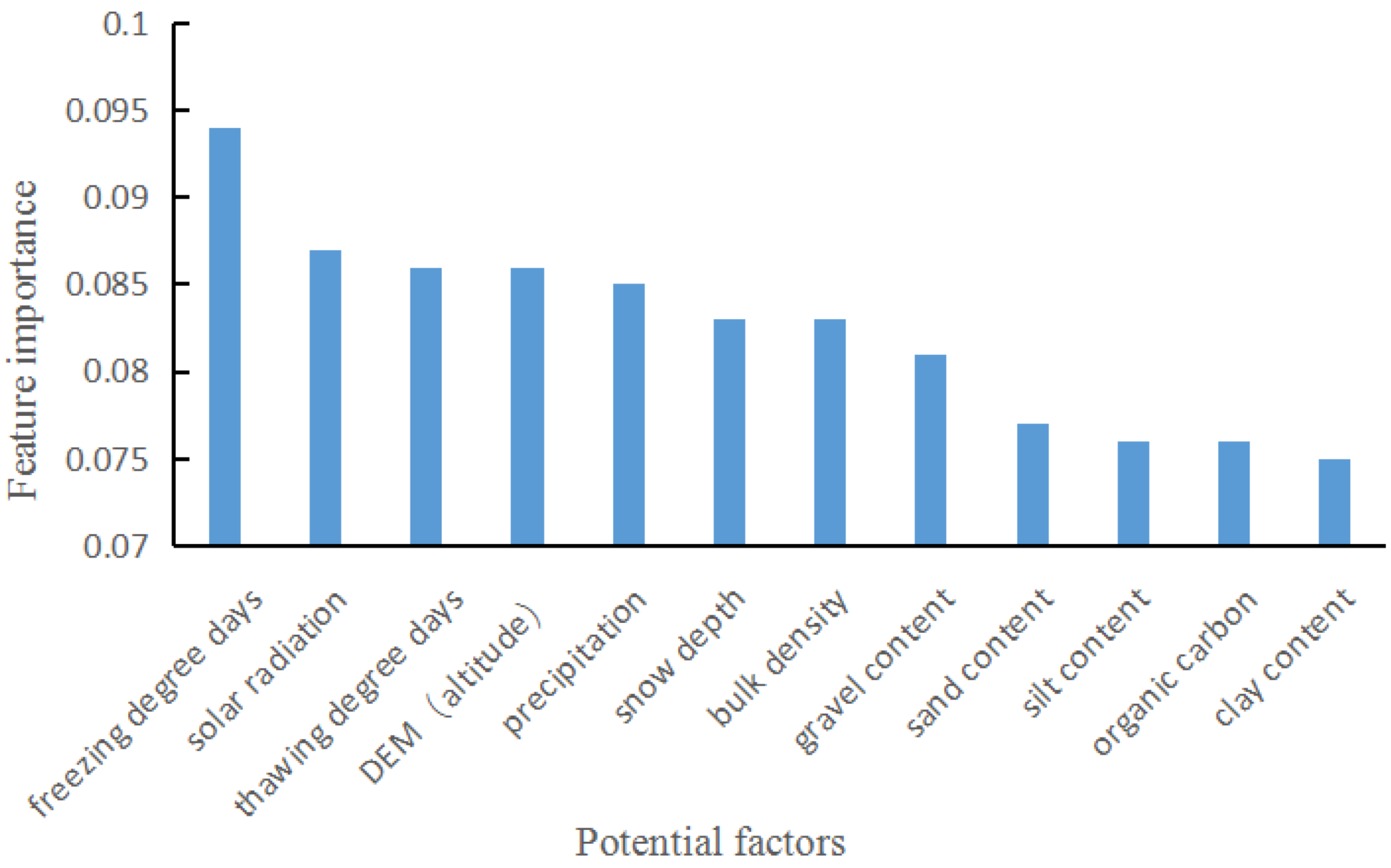
We used the extreme random tree method to rank the importance of 12 potential predictive factors: the freezing degree days, thawing degree days, snow depth, precipitation, solar radiation, DEM (altitude), and soil properties (bulk density, organic carbon, sand content, clay content, silt content, and gravel content). We selected the top-ranked predictive factor as the feature input variable [6]. The results are shown in Figure 2. The freezing degree days had the greatest impact on freezing depth, followed by solar radiation. The thawing degree days and DEM had roughly the same degree of impact on the freezing depth. The freezing degree days and thawing degree days were basic climate indicators. Climate change significantly impacts freezing depth [39,41,42]. The depth of snow cover and precipitation are also important factors affecting the seasonal freezing depth. Snow significantly isolates the energy exchange between the ground and the atmosphere. The thermal effect of frozen soil has changed, thereby affecting the freezing depth [28,40]. Precipitation changes the water content in frozen soil, bringing more surface heat into the soil. Among the soil elements, soil bulk density had the greatest impact on seasonal freezing depth, followed by gravel content. The clay content had the least impact on the seasonal freezing depth. This is consistent with research showing that the seasonal freezing depth distribution depends on the topography and lithology [43]. We optimized the prediction factors based on extreme random trees [6]. We sorted them according to the importance of the Gini factor, and selected the top-ranked features as the input variables. Ultimately, eight predictive factors were selected as feature input variables for MLM, namely: the freezing degree days, thawing degree days, solar radiation, DEM (altitude), snow depth, precipitation, soil bulk density, and gravel content.

3.2. Comparison of Machine-Learning Models (MLMs)

The four statistical learning modeling techniques used in this study included random forests (RF) [48], support vector machine regression (SVMR) [49], k-nearest neighbors (KNN) [50], and generalized linear regression (GLR). The techniques were implemented based on the scikit-learn module in Python [51]. RF is an ensemble-learning algorithm based on decision trees developed by Breiman. It uses bootstrap repetitive sampling and extracts samples from the total sample for modeling. The final output result is the average of the results of all decision trees. In this study, the number of trees was set to 100. Each tree was built using a randomly selected training dataset and environmental variables to split each tree node. SVMR features nonlinear kernel transformation, sparse solution, and maximal margin control [52]. It assumes that the maximum deviation (ε) between the predicted and measured values can be tolerated, and thus an ε-insensitive loss function can be found to minimize the prediction error. In this study, the default radial kernel function was used, and the grid search method based on 10-fold cross validation was used to select the model parameters. A normalization method was used to avoid overfitting. KNN found the k-nearest neighbors of each query point from the training sample and used the average of the k-nearest neighbors as the prediction target. In this study, the value of k was set to 10, and the value of weights was set to ‘distance’. GLR is a general extension of traditional linear regression. The loss function and regularization techniques were often used by GLR.
Remote sensing data and climate data are input variables. We used RF, SVMR, KNN, and GLR to construct MLMs. Each model was run 300–900 times. The results of 10-fold cross validation are shown in Table 3. From the R-squared, RMSE, MAE, and bias of each training frequency, it can be seen that the RF and SVMR methods were better than the KNN and GLR. Among the three indicators of RMSE, MAE, and bias, the indicator values of the RF and SVMR methods were significantly lower than those of the other two methods, indicating the advantages of the RF and SVMR methods for constructing MLMs. Using RF and SVMR, we compared the RMSE indicators of each training frequency. Although the RMSE of the RF method was lower than the corresponding value in the SVMR method, the MAE of each training frequency in SVMR was lower than the corresponding value of RF. Considering that the RMSE was more affected by outliers than MAE, the SVMR method with the smaller MAE was preferred when the RMSE indicators of the RF and SVMR methods were similar. Comparing the R-squared of each training frequency in SVMR and considering a sample size of 600, a support vector machine regression (SVMR) model with 600 learning iterations was adopted.

3.3. Evaluation of Machine-Learning Model Prediction Results

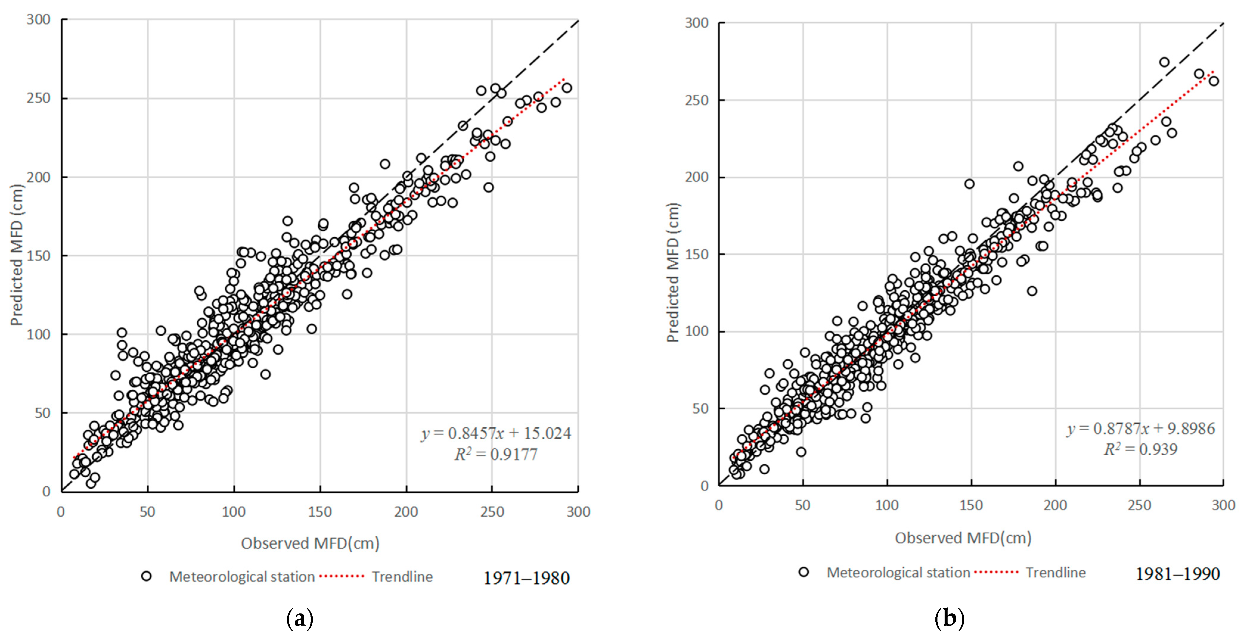
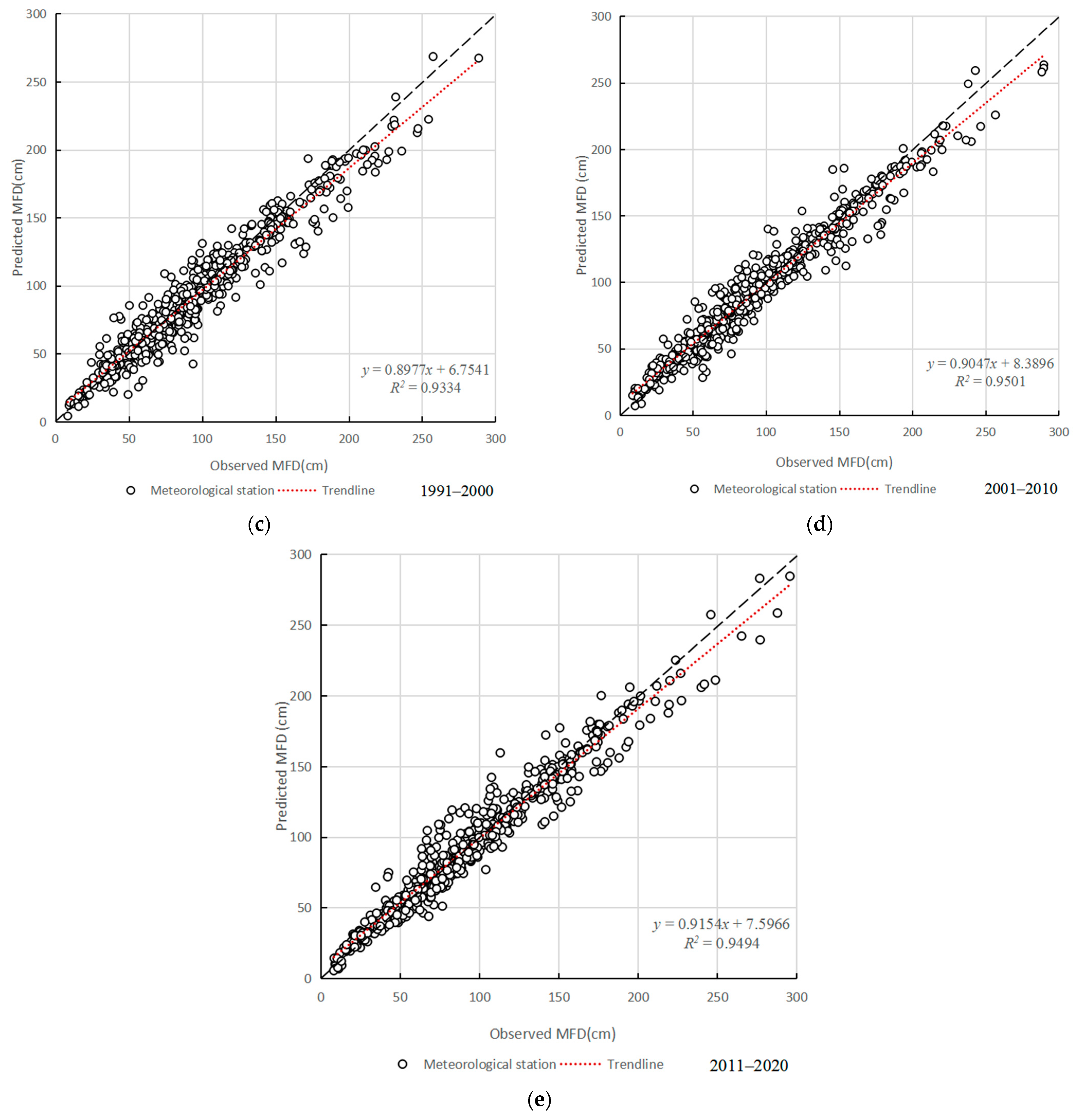
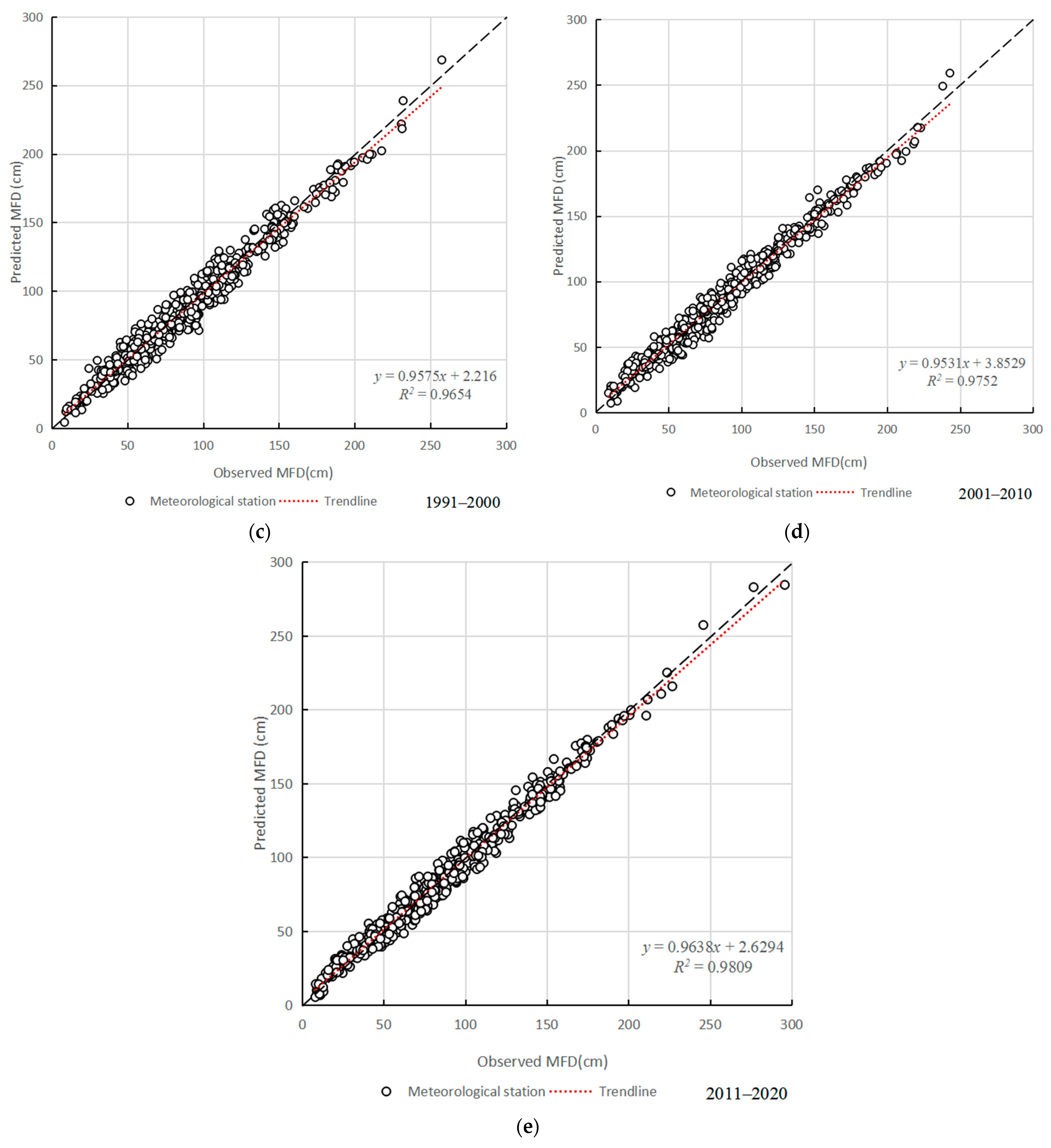
We extracted the average MFD prediction values of the meteorological monitoring points from the freezing depth map every 10 years from 1971 to 2020 and compared them to the average maximum values of the corresponding observation data. The comparison of the predicted values and observed values from 1971 to 2020 is shown in Figure 3.
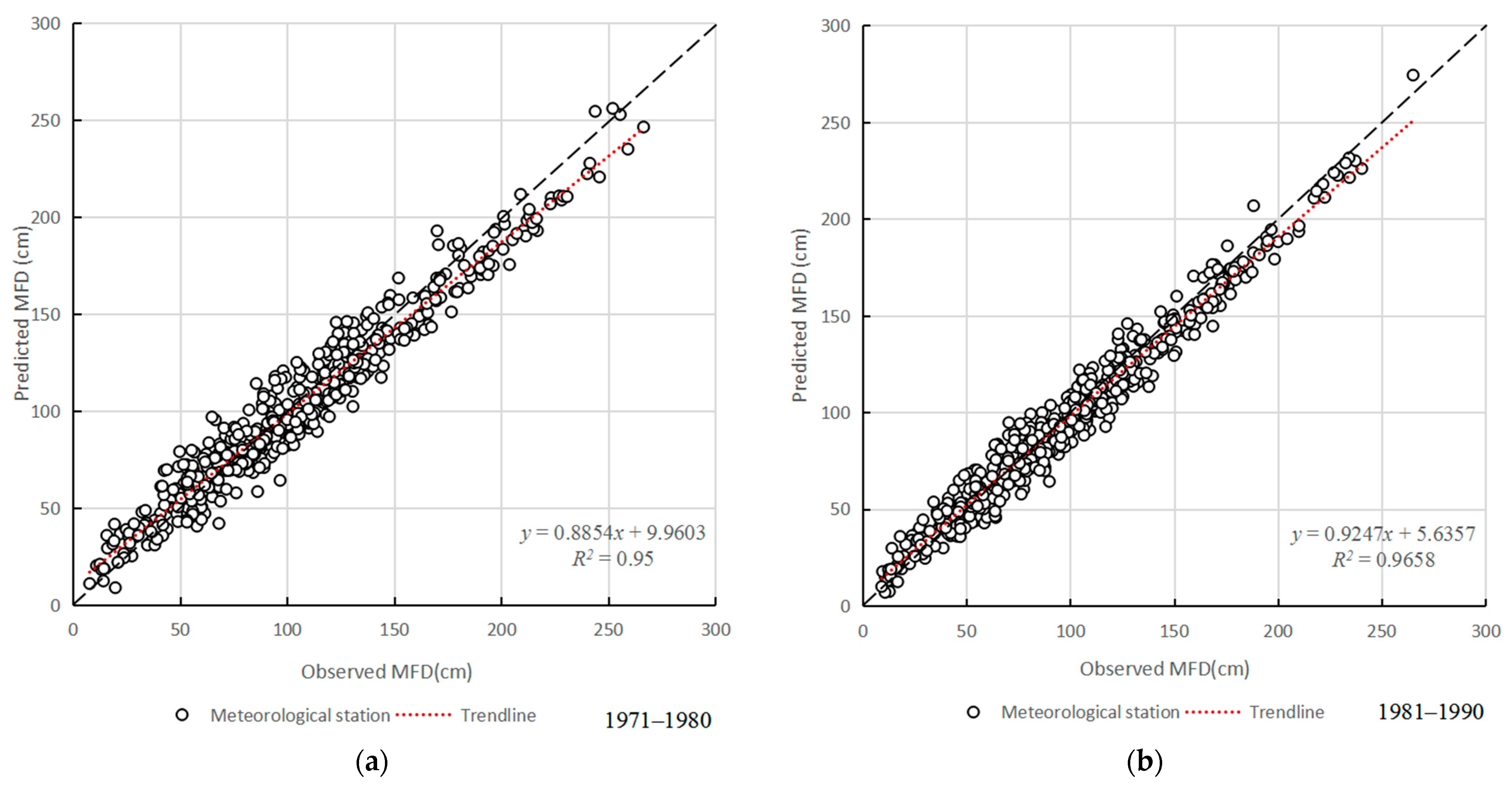
It can be seen that the predicted values and observed values fit well at most meteorological monitoring points. However, comparing the data in the graph, it was found that there was significant deviation between the predicted and observed values at some monitoring points. Through the comparison and analysis of the source data, it was found that these points with large deviations were usually distributed in the boundary zone between seasonally frozen ground and permafrost regions. This difference may be due to the existence of a transition zone at the boundary between seasonally frozen ground and permafrost. The frozen ground in the transition zone is generally in a state of mixed permafrost and seasonally frozen ground. The thermal stability of such soil and its geological conditions are not as good as other seasonally frozen ground regions. Geologic and geographical factors participate in the process of heat exchange between the lithosphere and the atmosphere to form seasonally frozen ground, restricting its development characteristics. Climate conditions are a basic control factor, and regional geological conditions play a decisive role in differences in seasonally frozen ground in the same region, especially at the edge of permafrost regions [53]. The poor thermal stability and the differential effect of geological conditions degenerate permafrost at the edge. The decrease in freezing depth of seasonal frozen soil was unstable, increasing the uncertainty of MLM simulations and causing prediction bias at certain monitoring points. As such, using MLMs to predict values in the transition zone could not effectively reflect the actual freezing depth. After removing the predicted values of these monitoring points in the transition zone, the average MFD predicted values of the meteorological monitoring points were compared with the average maximum values of the corresponding observation data, as shown in Figure 4. The predicted values fit well with the observed values and showed further improvement in the correlation coefficient, indicating that the accuracy of using MLM to predict the freezing depth of seasonally frozen ground region was good, except for the transition zone.

3.4. Overall Changing Trend of Maximum Freezing Depth

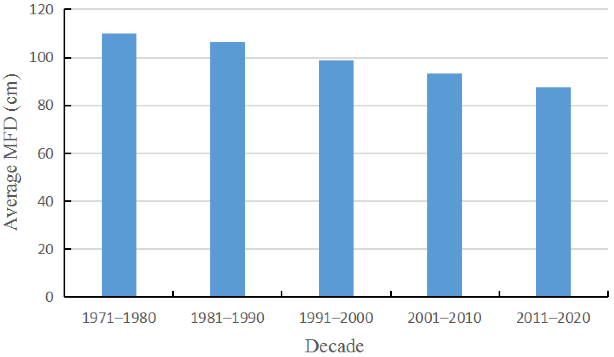
This study aimed to better understand the changes in freezing depth in China in the last 50 years. The average MFD in China during the interdecadal period is shown in Figure 5. From the graph, it can be seen that the average MFD in China decreased over the last 50 years. The average MFD in the 1970s, 1980s, 1990s, 2000s, and 2010s was 109.93 cm, 106.29 cm, 98.70 cm, 93.16 cm, and 87.58 cm, respectively. The average MFD in the 1980s, 1990s, 2000s, and 2010s was 3.64 cm, 7.59 cm, 5.54 cm, and 5.58 cm lower than in the previous decade, respectively. The freezing depth in the 1990s showed the greatest change: compared with the 1980s, the average MFD in the 1990s was reduced by 7.59 cm. Compared with the 1970s, the average MFD had the smallest change in the 1980s. The average MFD was reduced by 3.64 cm. After the 1990s, the average MFD in China remained relatively stable. The reduction in the average MFD between different decades remained about 5.5 cm.

3.5. Changes in Maximum Freezing Depth in Different Regions

We used MLM to predict the average MFD map for every decade from 1971 to 2020. The permafrost and lakes in the maps were masked. The permafrost region adopted the frozen ground map of China based on a map of the glaciers, frozen ground, and deserts in China [54]. The dataset was provided by the National Cryosphere Desert Data Center (http://www.ncdc.ac.cn (accessed on 1 March 2023)). The lake extent was derived from level 1 of the Global Lakes and Wetlands Database (GLWD; https://www.worldwildlife.org/ (accessed on 1 March 2023)) [55].
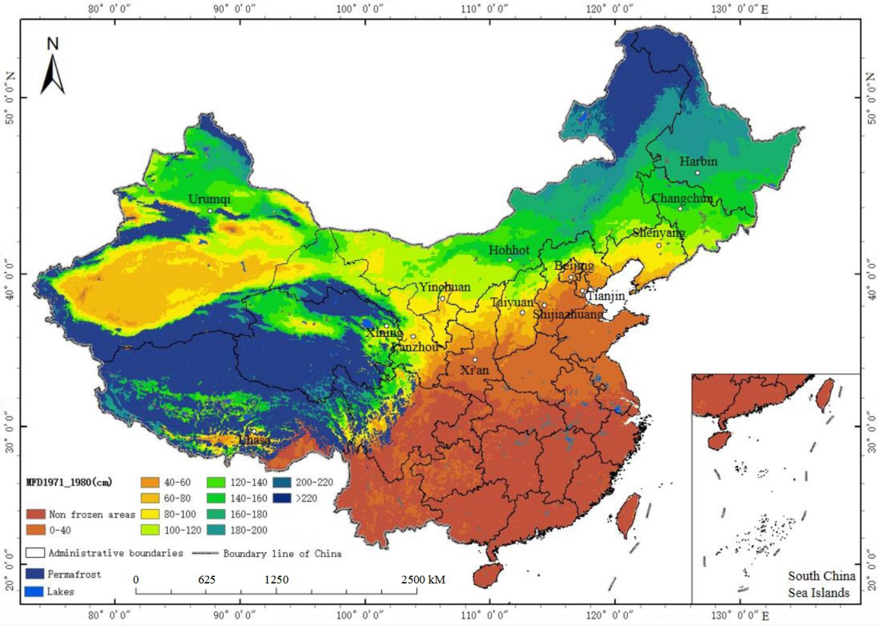
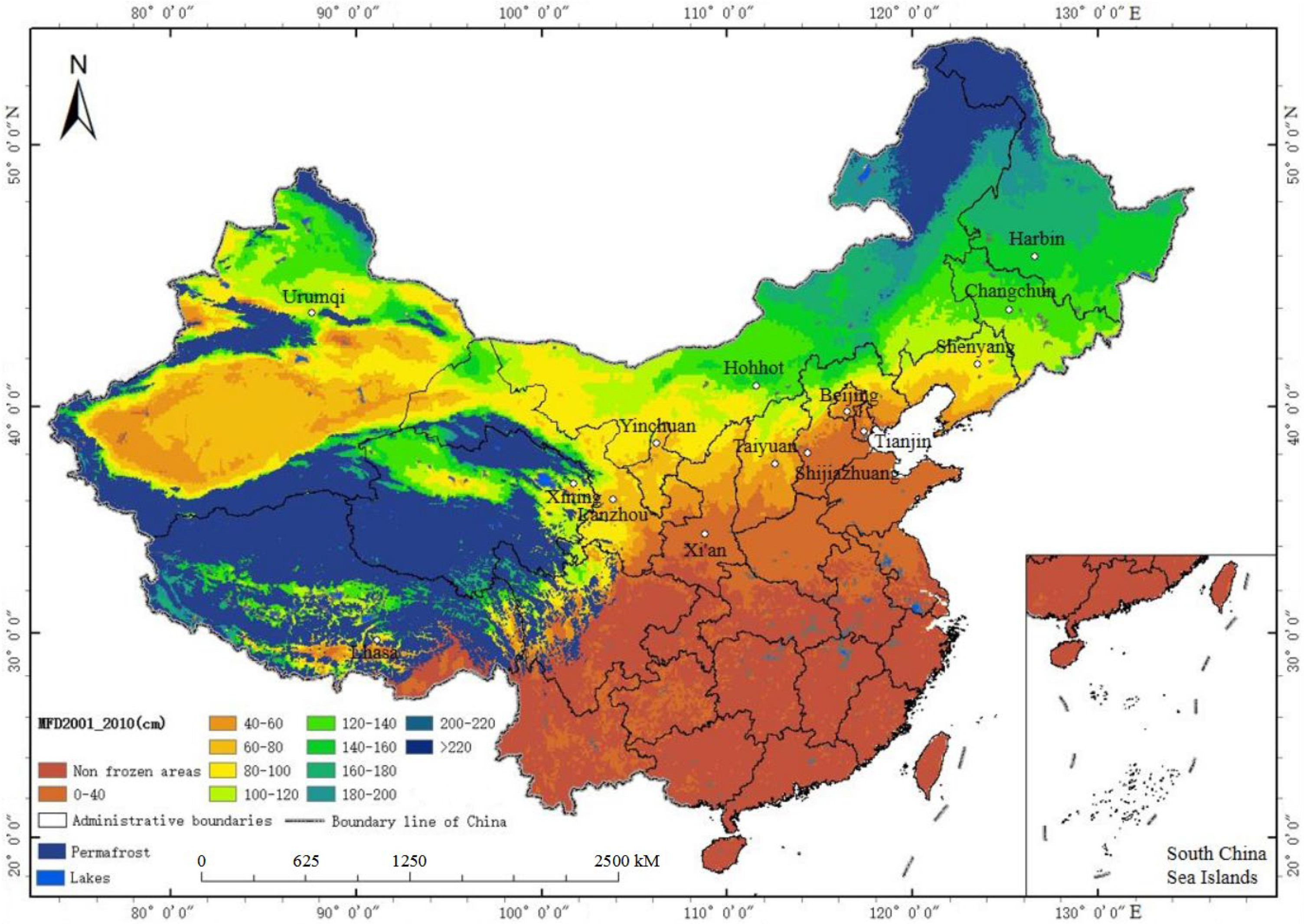
In the average MFD map from 1971 to 1980 (Figure 6), the 40 cm average MFD line in northern and northeast China started at around 39°N, with the longitude spanning from about 104°E–118°E. It passed through the central to southern parts of four provinces in China. As the longitude increased, the corresponding 40 cm average MFD line shifted towards northern China. The average MFD line of 60–80 cm started around 40°N–41°N, with the longitude spanning from approximately 104°E–125°E. The freezing depth line extended along southwest China, passing through the central and southern parts of four provinces in China. Most regions in these provinces had an MFD of 60–80 cm. The 100 cm MFD line started near 43°N, and its longitude spanned from about 100°E–127°E. The distribution of the 100 cm freezing depth line was relatively complex. The freezing depth line started in northeast China and spread along the southwest, passing through several provinces of northern and northwest China. At 39°N and 102°E, the freezing depth line extended southward along the eastern boundary of the permafrost region of the Qinghai-Tibet Plateau to the southeastern boundary. The starting points of the four average MFD lines, 120 cm, 140 cm, 160 cm, and 180 cm, were mainly concentrated from 40°N–48°N, with the longitude spanning from about 98°E–116°E. In northeastern China, the four average MFD lines were evenly arranged along the direction of latitude, increasing and extending westward in northern China. Among them, the 120 cm freezing depth line extended to 40°N and 103°E. The 140 cm and 160 cm freezing depth line extended to 41°N and 106°E, and the 180 cm freezing depth line extended to 44°N and 112°E. The average MFD line of 200 cm and above was adjacent to the boundary of the high-latitude permafrost region in northeastern China. The seasonal freezing depth values were generally large, and the average MFD in a few regions exceeded 220 cm. In the western and northwestern regions of China, the average MFD line was generally within the range of 60–160 cm. In a few regions, the average MFD line was between 160 cm and 220 cm. In the Tarim Basin (37°N–42°N, 85°E–94°E), there were mainly 60–160 cm freezing depth lines. The Tarim Basin is surrounded by the Tianshan Mountains and Kunlun Mountains. Each freezing depth line extended from the hinterland of the Tarim Basin to the permafrost region of the Qinghai−Tibet Plateau and the Tianshan permafrost region. The closer to the permafrost regions, the higher the freezing depth values. Within the range of 42°N–48°N and 80°E–96°E in northwest China, the geomorphic types mainly included the Junggar Basin (44°N–46°N, 82°E–89°E), Altai Mountains, and Tianshan Mountains. There were five freezing depth lines of 120–220 cm, which extended from the boundary of the Junggar Basin to the permafrost region of the Altai Mountains and Tianshan Mountains. Near the permafrost region, the freezing depth gradually increased. The average maximum freezing depth line of seasonally frozen ground (25°N–40°N, 74°E–104°E) around the permafrost region of the Qinghai-Tibet Plateau was mainly concentrated in the range of 40–220 cm. The Qaidam Basin is located to the north of the Qinghai−Tibet Plateau (35°N–40°N, 90°E–100°E). The freezing depth of seasonal frozen ground was mainly in the range of 120–220 cm, and some regions near the permafrost region had a depth of more than 220 cm. In addition, local regions in the hinterland of the Qaidam Basin generally had a freezing depth of 80–100 cm. At the southeast boundary of the permafrost region of the Qinghai−Tibet Plateau, there was a small amount of seasonally frozen ground in the island permafrost region. The freezing depth was 40–220 cm. The general rule was that the closer to the permafrost region, the greater the freezing depth.
The average MFD map from 1981 to 1990 (Figure 7) was compared to the map from 1971 to 1980. The freezing depth range of 60–80 cm had expanded in some regions between 42°N, 122°E and 38°N, 106°E. The freezing depth range of 80–100 cm expanded obviously in most regions within the range of 38°N–42°N and 98°E–104°E. In addition, the freezing depth in the vicinity of 42°N and 90°E decreased from 100–120 cm to the range of 80–100 cm. The freezing depth range of 100–120 cm expanded significantly near Changchun and Urumqi, followed by a reduction in the range of 120–140 cm near Changchun. The 120–140 cm freezing depth range of Urumqi gradually replaced the 140–160 cm freezing depth range, occupying most of the Junggar Basin (44°N–46°N,82°E–89°E) in northwest China. The freezing depth range of 160–180 cm was severely reduced within the range of 46°N–49°N and 130°E–134°E in northeast China. It was replaced by the freezing depth range of 140–160 cm. The freezing depth range of 160–180 cm near 48°N and 88°E was also reduced to varying degrees. The reduction in the freezing depth range of 180–200 cm near 46°N–50°N and 122°E–130°E in northeast China was very significant. Along the southern boundary of the permafrost region in northeast China, the freezing depth was reduced to 160–180 cm.
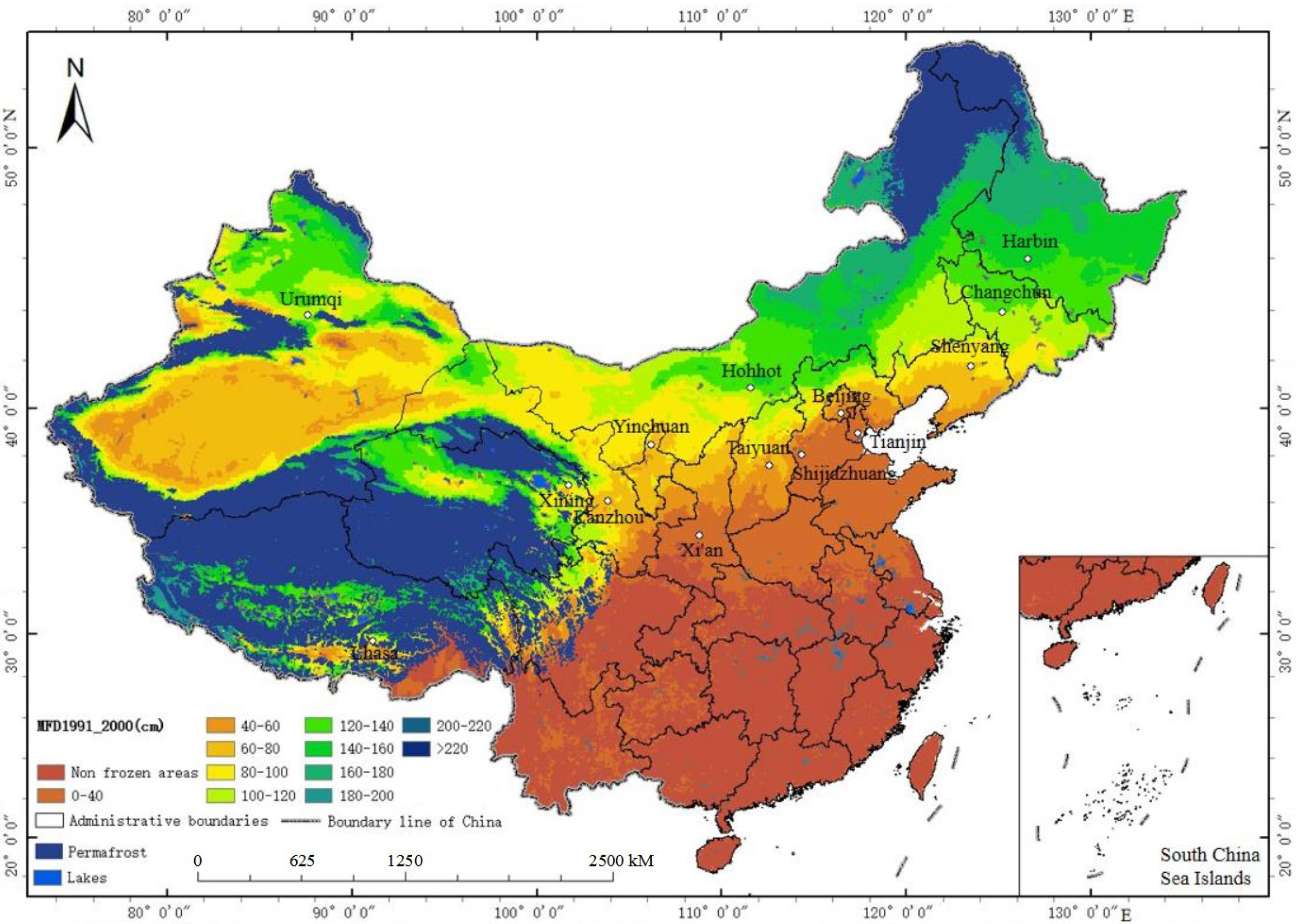
The average MFD map from 1991 to 2000 (Figure 8) was compared to the map from 1981 to 1990. Within the range of 42°N–46°N and 120°E–130°E, multiple freezing depth lines, such as 100 cm, 120 cm, 140 cm, and 160 cm, expanded to varying degrees to the north. Within 38°N–42°N and 98°E–104°E, the freezing depth range of 80–100 cm further expanded to the region near 110°E, and the freezing depth range of 100–120 cm continued to shrink. The freezing depth range of 200–220 cm near 50°N and 126°E sharply decreased compared with map of 1981–1990. In the Junggar Basin (44°N–46°N,82°E–89°E), the 120–140 cm freezing depth range was significantly reduced and replaced by the 100–120 cm freezing depth range.
The average MFD map from 2001 to 2010 (Figure 9) was compared to the map from 1991 to 2000. The freezing depth range of 60–80 cm covered all regions near 40°N–42°N and 120°E–126°E. The freezing depth range of 100–120 cm showed expansion in some regions, such as near 42°N108°E, 42°N127°E, and 44°N122°E, resulting in a reduction in the freezing depth range of 80–100 cm. The freezing depth range of 120–140 cm showed expansion near 44°N and 122°E–130°E, resulting in a decrease in the freezing depth range of 100–120 cm. Near 48°N–50°N and 122°E–128°E in the high latitude permafrost region of northeast China, the 180–200 cm freezing depth range increased to a certain extent. The freezing depth in some regions was more than 200 cm.
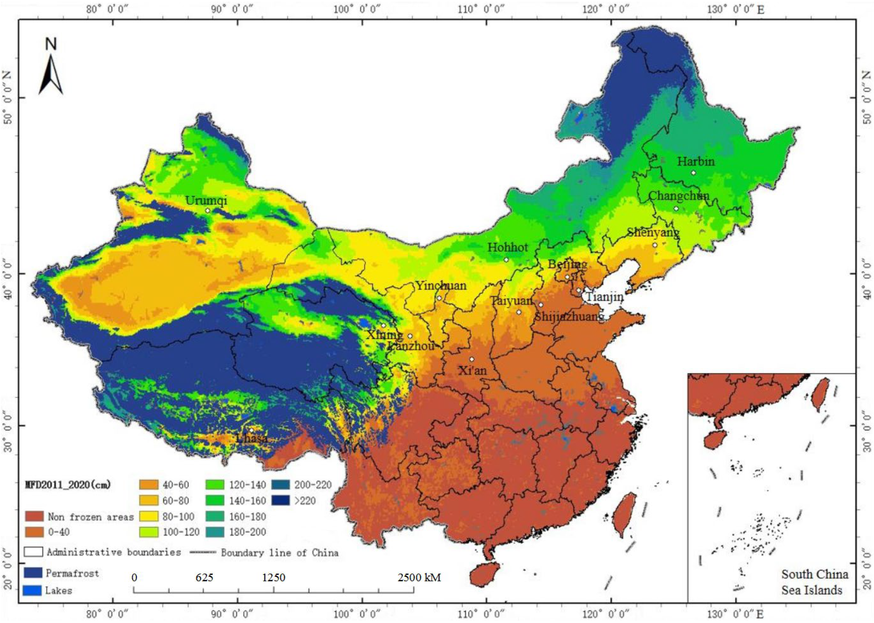
The average MFD map from 2011 to 2020 (Figure 10) was compared to the map from 2001 to 2010. Expansion occurred in local areas near 41°N and 124°E within the freezing depth range of 60–80 cm. The freezing depth range of 100–120 cm in some regions near 44°N and 120°E–130°E expanded north. The freezing depth range of 120–140 cm decreased. The freezing depth range of 120–140 cm expanded to a certain extent in the regions of 42°N–44°N and 84°E–89°E. The freezing depth range of 140–160 cm reduced to a certain extent around 44°N and 128°E. The freezing depth range of 160–180 cm decreased partially around 48°N and 130°E, and expanded locally in the 48°N and 88°E region. The freezing depth range of 180–200 cm decreased around 50°N and 126°E. We compared the average MFD of seasonally frozen ground in other regions of China, such as the Qinghai–Tibet Plateau (25°N–40°N, 74°E–104°E), the Tarim Basin (37°N–42°N, 85°E–94°E), and the Qaidam Basin (35°N–40°N, 90°E–100°E). The freezing depth of seasonal frozen ground did not change much from the average MFD from 2001 to 2010.
From the interdecadal average MFD map, it can be seen that the freezing depth changed more sharply within the range of 35°N–48°N, with the boundary lines of low freezing depth expanding sharply and the high freezing depth decreasing sharply. The boundary lines of 100 cm and 120 cm freezing depths in the central and northern regions of China were slightly degraded. They shrank in high latitudes in the north. The boundary lines of 40 cm, 60 cm, and 80 cm freezing depths expanded significantly, and the maximum freezing depth in the surrounding region decreased by 20–30 cm. The freezing depth boundary lines of 140 cm and above in the high latitude areas in northeast China was also reduced to varying degrees, with the most significant reduction being in the freezing depth boundary lines of 180 cm and 200 cm and above, followed by the more significant reduction in the freezing depth boundary lines of 160 cm. The freezing depth of seasonally frozen ground in the vicinity of Urumqi in northwest China varied significantly, with the range of the 80–100 cm freezing depth boundary continuously expanding and the 120 cm–140 cm range continuously decreasing. This is consistent with other research [56].

3.6. Area Variation of Seasonally Frozen Ground at Different Maximum Freezing Depths

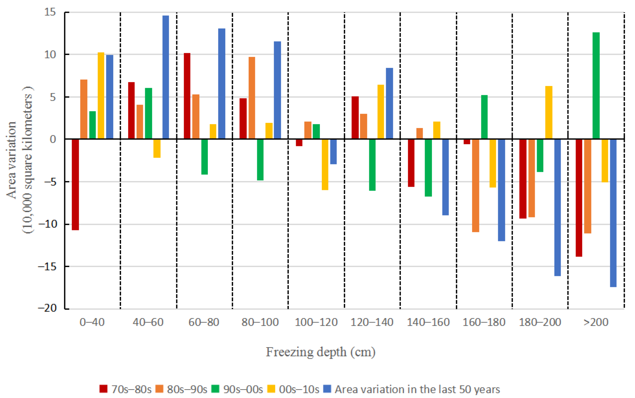
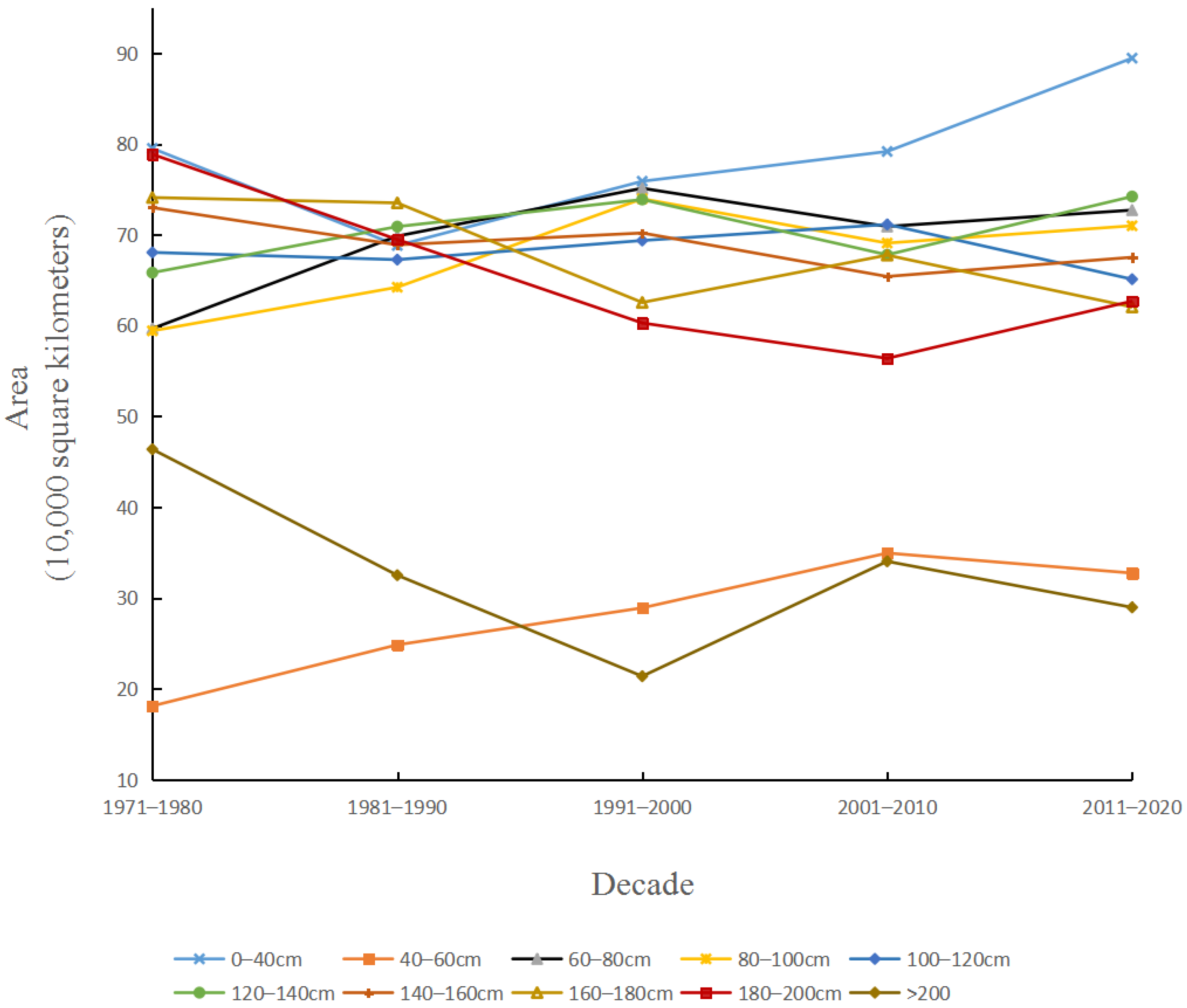
In the seasonally frozen ground region of China, we compared the interdecadal area occupied by each freezing depth range. The changes in area are shown in Figure 11 and Figure 12.
Through the area occupied by each freezing depth per decade in seasonally frozen ground (Figure 11), it can be seen that the freezing depth ranges of 0–60 cm and >180 cm changed considerably. The areas occupied by the other freezing depth ranges remained relatively stable. The interdecadal changes in the area of each freezing depth range are shown in Figure 12. It can be seen that in the last 50 years, the area of the freezing depth ranges of 0–40 cm, 40–60 cm, 60–80 cm, 80–100 cm, and 120–140 cm increased by 99,300 square kilometers, 146,200 square kilometers, 130,300 square kilometers, 115,600 square kilometers, and 83,800 square kilometers, respectively. The exception was a slightly decreased area in the 100–120 cm freezing depth range: the area was reduced by 29,500 square kilometers. The range of 40–60 cm frozen depth had the largest increase, followed by the range of 60–80 cm frozen depth. The range of 120–140 cm frozen depth showed the smallest increase. The freezing depth range greater than 140 cm showed a decreasing trend, with a reduction of 89,700 square kilometers in the area of the 140–160 cm freezing depth range—the smallest reduction in the freezing depth range. The freezing depth range of 160–180 cm decreased by 120,500 square kilometers, 180–200 cm decreased by 161,500 square kilometers, and the >200 cm range decreased by 174,000 square kilometers, the largest reduction in frozen depth range. The areas with small freezing depth values showed an overall increasing trend over the last 50 years, while areas with a large freezing depth values showed a decreasing trend. The MFD in the seasonally frozen ground region in China showed a decreasing trend year by year [57,58].

4. Discussion

There are many methods for calculating the seasonal freezing depth, among which the Stefan formula is the most widely used. The simplified Stefan formula has been applied for freezing depth estimation as it requires relatively few inputs [59,60]. However, the simplified Stefan formula does not fully consider the potential impact of DEM, snow depth, solar radiation, and precipitation on the seasonal freezing depth, which may limit its application in areas with a high latitude and high altitude. Because of the complex terrain and spatial heterogeneity across China, machine learning should improve the accuracy of seasonal freezing depth. We used a machine-learning model to predict the historical changes in seasonally frozen ground by considering the potential influences of driving factors (including the freezing index, melting index, DEM, snow depth, solar radiation, and precipitation) on MFD. The freezing index had the greatest impact on freezing depth, followed by solar radiation. The melting index and DEM had roughly the same degree of impact on the freezing depth [6]. The depth of snow cover and precipitation are also important factors affecting the seasonal freezing depth [28,41,61].
This research integrated the reanalysis data and observed the values from 600 meteorological stations to develop a machine-learning model to simulate MFD in seasonally frozen ground in China from 1971 to 2020. The accuracy of the machine-learning model was supported by the metrics (i.e., R-squared, RMSE, MAE, and bias) based on 10-fold cross validation. From the R-squared, RMSE, MAE, and bias of each training frequency, it can be seen that the SVMR method had a better spatial generalization ability. The predicted values fit well with the observed values. The SVMR method performed better in machine-learning simulations of seasonally frozen ground [60,61].
The trend of freezing depth decreased year by year affects the freeze/thaw state of seasonal soil and the distribution of seasonally frozen ground. The change in distribution and soil freeze/thaw state can also significantly affect climate ecosystems [62], such as carbon exchange between the atmosphere and the ground. The soil thaw state may result in the exposure of frozen carbon to microbial degradation and release active gases such as methane and carbon dioxide into the atmosphere [63]. Climate change is a significant worldwide concern. The idea of “carbon neutrality” opens up the possibility for a low-carbon future. The reduction in freezing depth affects the freeze/thaw state, leading to changes in carbon emissions. The research can provide a theoretical basis for the study of carbon distribution and carbon emission reduction.

5. Conclusions

This study optimized the impact factors of MFD on seasonally frozen ground. Based on a comparison of various machine-learning methods, we selected a model to predict the MFD in seasonally frozen ground. Meteorological observation data from 600 monitoring stations were compared with the predicted values to ensure the accuracy of the model’s predictions. The analysis of the model prediction results showed that the freezing depth of seasonally frozen ground in China decreased over the past 50 years due to the influence of climate factors, such as higher temperatures.
Maximum freezing depth changes in different regions: Each average MFD boundary line had a varying degree of deviation towards higher latitudes, with a large deviation in amplitude and impact range. The freezing depth range of 140 cm and below showed an increasing trend year by year, while the freezing depth range of 140 cm and above showed a decreased trend year by year. The freezing depth range of 200 cm and above had the greatest reduction. Overall, the expansion in the small freezing depth range was significant, while the reduction in the large freezing depth range was very significant. The expansion in the 80–100 cm freezing depth range was the most significant in the vicinity of 38°N–42°N, 100°E–110°E in northern China. The MFD in the surrounding regions decreased from 100–120 cm to 80–100 cm. The boundary line range of a 120–140 cm freezing depth near 44°N–46°N and 82°E–89°E in northwest China decreased year by year. The range of the freezing depth boundary line between 100 cm and 120 cm gradually expanded. The MFD in the surrounding regions also showed a decreasing trend year by year. In summary, the average MFD boundary line in the seasonally frozen ground region showed a strip distribution feature parallel to the latitude line, and it tilted from northeast to southwest China. The freezing depth decreased year by year, and the changes were significant.
This study adopts machine-learning methods. The ground data from 600 stations serves as a reference for the integration of all other data (MFD data, climate data, soil data, and DEM (altitude) data). The freezing depth data of seasonally frozen ground in China from 1971 to 2020 are considered. The data are used to study freezing depth changes. The results of the study are not limited to single-point observation data from surface meteorological stations. In remote areas, observational data are lacking, and the results complement the regional data well. In addition, considering the lack of data on the change in the MFD of seasonally frozen ground in China in recent decades, the results of this study can provide the necessary basis for research and support for other researchers.
In this study, machine learning improves the estimation of maximum freezing depth based on re-analyzing climate input variables. The results show that the predicted and observed values are in good agreement. In addition, considering the transition zone between the permafrost region and the seasonally frozen ground region, the difference in geological and geographical conditions and the poor thermal stability of frozen soil increase the uncertainty of the machine-learning model’s simulation. This results in deviations in the predictions of the freezing depth at monitoring points in the transition zone. Thus, other methods can be considered to study changes in the freezing depth on the transition zone, which is our next research plan. Vast quantities of observational data are gathered on the Earth every day, including from satellites, sensors, drones, and non-traditional social sensing data [64]. Advances in machine learning have been marked by the development of deep learning and other methods. These methods are more capable of solving a series of high dimensionality, complexity, and nonlinear problems in Earth science [65,66]. In the future, MFD simulations could be improved in at least two ways: through remote sensing variables and model structures. Multiple deep-learning architectures, such as convolutional neural networks, might be promising to promote MFD simulation. More remote sensing variables, such as Landsat data, have the potential to improve the accuracy of MFD simulations.

Author Contributions

Validation, B.W.; investigation, E.P. and C.P.; resources, Y.R.; writing—original draft preparation, S.W.; writing—review and editing, Y.S. and Y.R.; supervision, Y.S.; project administration, W.C. All authors have read and agreed to the published version of the manuscript.

Funding

This research was funded by the China National Natural Science Foundation (No. 41971093, and No. 52068035).

Data Availability Statement

The data presented in this study are available on request from the corresponding author.

Acknowledgments

The authors are grateful to the editors and anonymous reviewers for their insightful comments and suggestions that helped improve this paper.

Conflicts of Interest

The authors declare no conflict of interest.

References

  1. Zhou, Y.W.; Guo, D.X.; Qiu, G.Q.; Cheng, G.; Li, S. Geocryology in China, 1st ed.; Science Press: Beijing, China, 2000; pp. 9–19. [Google Scholar]
  2. Yang, J.P.; Yang, S.Q.; Li, M. Vulnerability of permafrost to climate change in China. J. Glaciol. Geocryol. 2013, 35, 10–15. [Google Scholar]
  3. Zhao, L.; Cheng, G.D.; Ding, Y.J. Studies on frozen ground of China. J. Geogr. Sci. 2004, 14, 411–416. [Google Scholar]
  4. Qin, Y.; Chen, J.; Yang, D.; Wang, T. Estimating seasonally frozen ground depth from historical climate data and site measurements using a Bayesian model. Water Resour. Res. 2018, 54, 4361–4375. [Google Scholar] [CrossRef]
  5. Choi, H.J.; Kim, S.; Kim, Y.; Won, J. Predicting Frost Depth of Soils in South Korea Using Machine Learning Techniques. Sustainability 2022, 14, 9767. [Google Scholar] [CrossRef]
  6. Wang, B.; Ran, Y. Diversity of remote sensing-based variable inputs improves the estimation of seasonal maximum freezing depth. Remote Sens. 2021, 13, 4829. [Google Scholar] [CrossRef]
  7. Lary, D.J.; Alavi, A.H.; Gandomi, A.H.; Walker, A.L. Machine learning in geosciences and remote sensing. Geosci. Front. 2016, 7, 3–10. [Google Scholar] [CrossRef] [Green Version]
  8. Song, X.; Guo, L.F.; Rao, M.N. Machine learning approaches to multisource geospatial data classification: Application to CRP mapping in Texas County, Oklahoma. In IEEE Workshop on Advances in Techniques for Analysis of Remotely Sensed Data; IEEE: New York, NY, USA, 2003. [Google Scholar]
  9. Bhattacharya, B.; Solomatine, D.P. Machine learning in soil classification. Neural Netw. 2006, 19, 186–195. [Google Scholar] [CrossRef]
  10. Wang, B.Q.; Ran, Y.H. Decadal dataset of the seasonal maximum freezing depth with 1 km resolution from 1961 to 2020 in Northwest China, Tibet and surrounding area. Adv. Ear. Sci. 2021, 36, 1137–1145. [Google Scholar]
  11. Alizamir, M.; Kisi, O.; Ahmed, A.N.; Mert, C.; Fai, C.M.; Kim, S.; Kim, N.W.; El-Shafie, A. Advanced machine learning model for better prediction accuracy of soil temperature at different depths. PLoS ONE 2020, 15, e0231055. [Google Scholar] [CrossRef] [Green Version]
  12. Ran, Y.-H.; Li, X.; Che, T.; Wang, B.-Q.; Cheng, G.-D. Current state and past changes in frozen ground at the Third Pole: A research synthesis. Adv. Clim. Chang. Res. 2022, 13, 4–11. [Google Scholar] [CrossRef]
  13. Wang, B.Q.; Ran, Y.H. Machine learning-based forecasting of future maximum freezing depth over the Third Pole. J. Glaciol. Geocryol. 2023, 45, 1–10. [Google Scholar]
  14. Sha, L.; Zhang, Y.M. Research on automatic observation methods of freezing depth in Shenyang, China. Meteorol. Hydrol. Mar. Instrum. 2019, 36, 56–59. [Google Scholar]
  15. Liu, T.L. An overview of formulas for calculating freezing or thawing depth. J. Glaciol. Geocryol. 1983, 2, 85–95. [Google Scholar]
  16. DeGaetano, A.T.; Cameron, M.D.; Wilks, D.S. Physical simulation of maximum seasonal soil freezing depth in the United States using routine weather observations. J. Appl. Meteorol. 2001, 40, 546–555. [Google Scholar] [CrossRef]
  17. Godlewski, T.; Wodzyński, Ł.; Wszędyrówny-Nast, M. Probabilistic analysis as a method for ground freezing depth estimation. Appl. Sci. 2021, 11, 8194. [Google Scholar] [CrossRef]
  18. Jerzy, A.U.; Sobolewski, A. Probabilistic approach to the assessment of the depth of soil freezing. In Proceedings of the 13th Baltic Sea Region Geotechnical Conference, Vilnius, Lithuania, 22–24 September 2016. [Google Scholar]
  19. Kudriyatsev, B.A.; Guo, D.X.; Ma, S.M.; Ding, D.W. Principles of Frozen Soil Prediction in Engineering Geological Research, 1st ed.; Lanzhou University Press: LanZhou, China, 1992; pp. 112–123. [Google Scholar]
  20. Friedman, G.M.; Cheng, G.D.; Ding, D.W. Calculation Method for Temperature Conditions of Frozen Soil, 1st ed.; Science Press: Beijing, China, 1982; pp. 15–23. [Google Scholar]
  21. Institute of Frozen Soil Research, Siberian Branch of the Soviet Academy of Sciences. General Frozen Soil Science, 1st ed.; Science Press: Beijing, China, 1988; pp. 21–29. [Google Scholar]
  22. Degaetano, A.T.; Wilks, D.S. Extreme-value climatology of maximum soil freezing depths in contiguous United States. J. Cold Reg. Eng. 2002, 16, 51–71. [Google Scholar] [CrossRef]
  23. Guo, D. Simulation of permafrost and seasonally frozen ground conditions on the Tibetan Plateau, 1981–2010. J. Geophys. Res-Atmos. 2013, 118, 5216–5230. [Google Scholar] [CrossRef]
  24. Saito, K.; Emori, S.; Kimoto, M. Change in hydro-thermal regimes in the soil-freezing regions in the Global Warming simulation by a CGCM of moderate- and high-resolution. In Proceedings of the Asian Conference on Permafrost, Lanzhou, China, 7–9 August 2006. [Google Scholar]
  25. Lawrence, D.M.; Slater, A.G.; Swenson, S.C. Simulation of present-day and future permafrost and seasonally frozen ground conditions in CCSM4. J. Clim. 2012, 25, 2207–2225. [Google Scholar] [CrossRef] [Green Version]
  26. Duguay, R.; Pietroniro, A. Remote Sensing in Northern Hydrology: Measuring Environmental Change, 1st ed.; American Geophysical Union: Washington, DC, USA, 2005; Volume 163, pp. 91–118. [Google Scholar]
  27. Walter, G.R.; Stothoff, S.A.; Necsoiu, D.M.; Dinwiddie, C.L. Integrated methodology for mapping and monitoring permafrost and seasonally frozen ground. In Proceedings of the Society of Petroleum Engineers-Arctic Technology Conference, Houston, TX, USA, 7–9 February 2011. [Google Scholar]
  28. Rey, D.M.; Hinckley, E.L.S.; Walvoord, M.A.; Singha, K. Integrating observations and models to determine the effect of seasonally frozen ground on hydrologic partitioning in alpine hillslopes in the Colorado Rocky Mountains, USA. Hydrol. Process. 2021, 35, e14374. [Google Scholar] [CrossRef]
  29. Traczyk, A.; Migaa, K. Depth of seasonally frozen ground in the Karkonosze Mts (Sudetes, SW Poland) in the light of GIS modeling of topoclimate and geomorphic conditions. XI. In Proceedings of the International Conference on Permafrost, Potsdam, Germany, 3–5 June 2016. [Google Scholar]
  30. Gouttevin, I.; Krinner, G.; Ciais, P.; Polcher, J.; Legout, C. Multi-scale validation of a new soil freezing scheme for a land-surfacemodel with physically-based hydrology. Cryosphere 2012, 6, 407–430. [Google Scholar] [CrossRef] [Green Version]
  31. Walvoord, M.A.; Kurylyk, B.L. Hydrologic impacts of thawing permafrost-a review. Vadose. Zone J. 2016, 15, 1–20. [Google Scholar] [CrossRef] [Green Version]
  32. Ran, Y.; Li, X. Progress, Chanllenges and opportunities of permafrost mapping in China. Adv. Earth Sci. 2019, 34, 1015–1027. [Google Scholar]
  33. Sabaghy, S.; Walker, J.P.; Renzullo, L.J.; Jackson, T.J. Spatially enhanced passive microwave derived soil moisture: Capabilities and opportunities. Remote Sens. Environ. 2018, 209, 551–580. [Google Scholar] [CrossRef]
  34. Minha, C.; Yoomi, H. A microwave-optical/infrared disaggregation for improving spatial representation of soil moisture using AMSR-E and MODIS products. Remote Sens. Environ. 2012, 124, 259–269. [Google Scholar]
  35. Wang, L.; Fang, S.; Pei, Z.; Wu, D.; Zhu, Y.; Zhuo, W. Developing machine learning models with multisource inputs for improved land surface soil moisture in China. Comput. Electron. Agric. 2022, 192, 106623. [Google Scholar] [CrossRef]
  36. Mehmet, B. Prediction of soil temperature using regression and artificial neural network models. Meteorol. Atmos. Phys. 2010, 110, 59–70. [Google Scholar]
  37. Feng, Y.; Cui, N.B.; Hao, W.P.; Gao, L.L.; Gong, D.Z. Estimation of soil temperature from meteorological data using different machine learning models. Geoderma 2019, 338, 67–77. [Google Scholar] [CrossRef]
  38. Nahvi, B.; Habibi, J.; Mohammadi, K.; Shamshirband, S.; Al Razgan, O.S. Using self-adaptive evolutionary algorithm to improve the performance of an extreme learning machine for estimating soil temperature. Comput. Electron. Agric. 2016, 124, 150–160. [Google Scholar] [CrossRef]
  39. Kalyuzhny, I.L.; Lavrov, S.A. Effect of climate changes on the soil freezing depth in the Volga River basin. Led. Sneg. Ice Snow 2016, 56, 437–451. [Google Scholar] [CrossRef]
  40. Zhang, W.; Shen, Y.; Wang, X.; Kang, S.; Chen, A.A.; Mao, W.; Zhong, X. Snow cover controls seasonally frozen ground regime on the southern edge of Altai Mountains. Agric. For. Meteorol. 2021, 297, 108271. [Google Scholar] [CrossRef]
  41. Qin, Y.; Lei, H.M.; Yang, D.W.; Gao, B.; Wang, Y.H.; Cong, Z.T.; Fan, W.J. Long-term change in the depth of seasonally frozen ground and its ecohydrological impacts in the Qilian Mountains, northeastern Tibetan Plateau. J. Hydrol. 2016, 9, 8–26. [Google Scholar] [CrossRef]
  42. Frauenfeld, O.W. Interdecadal changes in seasonal freeze and thaw depths in Russia. J. Geophys. Res. 2004, 109, D05101. [Google Scholar] [CrossRef]
  43. Nella, S. Specific features of distribution of the perennially and seasonally frozen ground in Transbaikalia. In Proceedings of the Asian Conference on Permafrost, Lanzhou, China, 7–9 August 2006. [Google Scholar]
  44. Sahbeni, G.; Pleynet, J.B.; Jarocki, K. A spatiotemporal analysis of precipitation anomalies using rainfall Gini index between 1980 and 2022. Atmos. Sci. Lett. 2023, 24, e1161. [Google Scholar] [CrossRef]
  45. Ceriani, L.; Verme, P. The origins of the Gini index: Extracts from variabilità e mutabilità (1912) by Corrado Gini. J. Econ. Inequal. 2012, 10, 421–443. [Google Scholar] [CrossRef]
  46. Muñoz-Sabater, J.; Dutra, E.; Agustí-Panareda, A.; Albergel, C.; Arduini, G.; Balsamo, G.; Boussetta, S.; Choulga, M.; Harrigan, S.; Hersbach, H.; et al. ERA5-Land: A state-of-the-art global reanalysis dataset for land applications. Earth Syst. Sci. Data 2021, 13, 4349–4383. [Google Scholar] [CrossRef]
  47. Wang, S.G.; Dai, Y.; Duan, Q.; Liu, B.; Yuan, H. A global soil data set for earth system modeling. J. Adv. Model. Earth Syst. 2014, 6, 249–263. [Google Scholar]
  48. Breiman, L. Random forests. Mach. Learn. 2001, 45, 5–32. [Google Scholar] [CrossRef] [Green Version]
  49. Vapnik, V. The Nature of Statistical Learning Theory; Springer: New York, NY, USA, 1995. [Google Scholar]
  50. Zhang, M.L.; Zhou, Z.H. ML-KNN: A lazy learning approach to multi-label learning. Pattern Recognit. 2007, 40, 2038–2048. [Google Scholar] [CrossRef] [Green Version]
  51. Pedregosa, F.; Varoquaux, G.; Gramfort, A.; Michel, V.; Thirion, B.; Grisel, O.; Blondel, M.; Prettenhofer, P.; Weiss, R.; Dubourg, V. Scikit-Learn: Machine Learning in Python. J. Mach. Learn. Res. 2011, 12, 2825–2830. [Google Scholar]
  52. Awad, M.; Khanna, R. Support Vector Regression in Efficient Learning Machines; APress: Berkeley, CA, USA, 2015; pp. 25–31. [Google Scholar]
  53. Tong, B.L.; Xie, Y.Q.; Guo, D.X. Seasonal permafrost at the southern foot of Tanggula Mountain. Glacier Permafr. 1980, 2, 23–28. [Google Scholar]
  54. Wang, T. Distribution Map of Frozen Soil in China Based on the “Map of Glaciers, Frozen Soil, and Deserts in China”; National Glacier, Frozen Soil and Desert Science Data Center: Lanzhou China, 2019. [Google Scholar]
  55. Lehner, B.; Döll, P. Development and validation of a global database of lakes, reservoirs and wetlands. J. Hydrol. 2004, 296, 1–22. [Google Scholar] [CrossRef]
  56. Liu, X.N.; Li, Q.X. Variation and preliminary interpretation of the maximum frozen soil depth in China. J. Appl. Meteorol. Sci. 2003, 14, 299–308. [Google Scholar]
  57. Chen, B. Temporal and Spatial Variation Characteristics of Frozen Soil in China and Its Relationship with East Asian Climate. Master’s Thesis, Institute of Atmospheric Physics, Chinese Academy of Sciences, Beijing, China, 2007. [Google Scholar]
  58. Wang, X.; Chen, R.; Han, C.; Yang, Y.; Liu, J.; Liu, Z.; Guo, S. Estimation of soil freeze depth in typical snowy regions using reanalysis dataset: A case study in Heilongjiang province, China. Remote Sens. 2022, 14, 5989. [Google Scholar] [CrossRef]
  59. Peng, X.; Zhang, T.; Frauenfeld, O.W.; Wang, K.; Cao, B.; Zhong, X.; Su, H.; Mu, C. Response of seasonal soil freeze depth to climate change across China. Cryosphere 2017, 11, 1059–1073. [Google Scholar] [CrossRef] [Green Version]
  60. Wang, T.; Yang, D.; Fang, B.; Yang, W.; Qin, Y.; Wang, Y. Data-driven mapping of the spatial distribution and potential changes of frozen ground over the Tibetan Plateau. Sci. Total Environ. 2019, 649, 515–525. [Google Scholar] [CrossRef]
  61. Ran, Y.; Li, X.; Cheng, G.; Nan, Z.; Che, J.; Sheng, Y.; Wu, Q.; Jin, H.; Luo, D.; Tang, Z.; et al. Mapping the permafrost stability on the Tibetan Plateau for 2005–2015. Sci. China Earth Sci. 2020, 64, 62–79. [Google Scholar] [CrossRef]
  62. Zhang, T.; Armstrong, R.; Smith, J. Investigation of the near-surface soil freeze-thaw cycle in the contiguous United States: Algorithm development and validation. J. Geophys. Res. 2003, 108, 8860. [Google Scholar] [CrossRef] [Green Version]
  63. Zimov, S.A.; Schuur, E.A.; Chapin, F.S., III. Permafrost and the global carbon budget. Science 2006, 312, 1612–1613. [Google Scholar] [CrossRef]
  64. Li, X.; Feng, M.; Ran, Y.H.; Su, Y.; Liu, F.; Huang, C.; Guo, H. Big Data in Earth system science and progress towards a digital twin. Nat. Rev. Earth Env. 2023, 5, 319–332. [Google Scholar] [CrossRef]
  65. Hinton, G.E.; Osindero, S.; Teh, Y.W. A fast learning algorithm for deep belief nets. Neural Comput. 2006, 18, 1527–1554. [Google Scholar] [CrossRef]
  66. Hinton, G.E.; Salakhutdinov, R.R. Reducing the dimensionality of data with neural networks. Science 2006, 313, 504–507. [Google Scholar] [CrossRef] [Green Version]
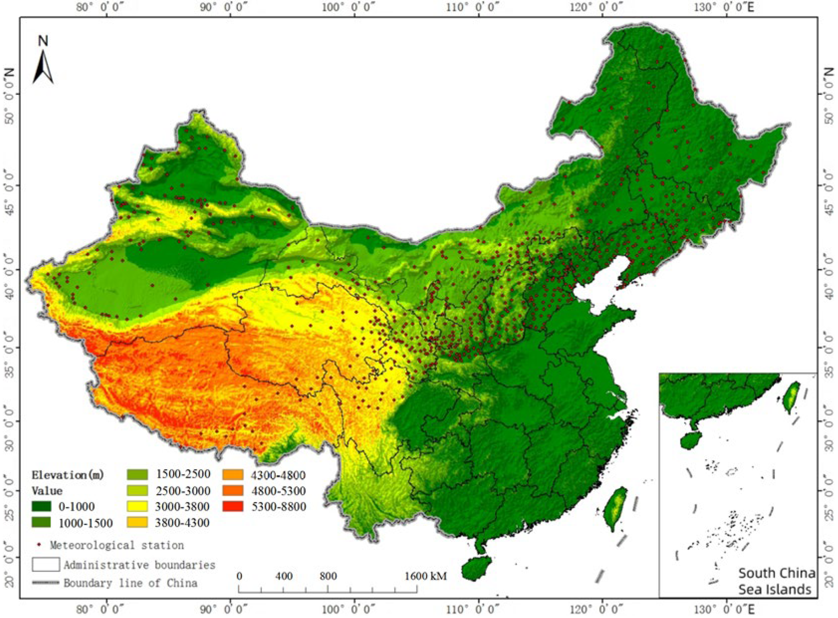
Figure 1. Spatial distribution map of all meteorological monitoring points.
Remotesensing 15 03834 g001
Figure 2. Ranking the importance of the input variables.
Remotesensing 15 03834 g002
Figure 3. Comparison of predicted and observed values from 1971 to 2020: (a) 1971–1980, (b) 1981–1990, (c) 1991–2000, (d) 2001–2010, and (e) 2011–2020.
Remotesensing 15 03834 g003aRemotesensing 15 03834 g003b
Figure 4. Comparison of predicted and observed values from 1971 to 2020 (revised). The meteorological stations in the transition zone were not taken into account: (a) 1971–1980, (b) 1981–1990, (c) 1991–2000, (d) 2001–2010, and (e) 2011–2020.
Remotesensing 15 03834 g004aRemotesensing 15 03834 g004b
Figure 5. Average maximum freezing depth in China by decade.
Remotesensing 15 03834 g005
Figure 6. Map of average maximum freezing depth from 1971 to 1980.
Remotesensing 15 03834 g006
Figure 7. Map of average maximum freezing depth from 1981 to 1990.
Remotesensing 15 03834 g007
Figure 8. Map of average maximum freezing depth from 1991 to 2000.
Remotesensing 15 03834 g008
Figure 9. Map of average maximum freezing depth from 2001 to 2010.
Remotesensing 15 03834 g009
Figure 10. Map of average maximum freezing depth from 2011 to 2020.
Remotesensing 15 03834 g010
Figure 11. Comparison of the interdecadal area occupied by each freezing depth range.
Remotesensing 15 03834 g011
Figure 12. Changes in the area of each freezing depth range (10,000 km2).
Remotesensing 15 03834 g012
Table 1. Environmental and climate variable datasets and DEM used in this study.
VariableDate Source and ReferenceSpatial ResolutionTemporal Resolution
and Time Span
Freezing degree days, °C·daysERA5-Land, Muñoz-Sabater et al. [46]9 kmDaily, 1971–2020
Thawing degree days, °C·daysERA5-Land, Muñoz-Sabater et al. [46]9 kmDaily, 1971–2020
Precipitation, mERA5-Land, Muñoz-Sabater et al. [46]9 kmDaily, 1971–2020
Snow depth, mERA5-Land, Muñoz-Sabater et al. [46]9 kmDaily, 1971–2020
Solar radiation, J m 2 d 1 ERA5-Land, Muñoz-Sabater et al. [46]9 kmDaily, 1971–2020
Soil bulk density, g / c m 3 GSDE, Shangguan W et al. [47]1 km-
Soil organic carbon, % of weightGSDE, Shangguan W et al. [47]1 km-
Sand content, % of weightGSDE, Shangguan W et al. [47]1 km-
Clay content, % of weightGSDE, Shangguan W et al. [47]1 km-
Silt content, % of weightGSDE, Shangguan W et al. [47]1 km-
Gravel content, % of volumeGSDE, Shangguan W et al. [47]1 km-
DEM (altitude), mASTER GDEM 30 m30 m-
Table 2. The resolution of resampled data.
VariableOriginal
Resolution
Resolution
after Downscaling
Freezing degree days, °C·days9 km9 km (no change)
Thawing degree days,°C·days9 km9 km (no change)
Precipitation, m9 km9 km (no change)
Snow depth, m9 km9 km (no change)
Solar radiation, J m 2 d 1 9 km9 km (no change)
Soil bulk density, g / c m 3 1 km9 km
Soil organic carbon, % of weight1 km9 km
Sand content, % of weight1 km9 km
Clay content, % of weight1 km9 km
Silt content, % of weight1 km9 km
Gravel content, % of volume1 km9 km
DEM (altitude), m30 m9 km
Table 3. Mean values and standard deviation of statistical indicators of various machine-learning models.
Learning TimesStatistical IndicatorsRFSVMRKNNGLR
Mean Values/Standard Deviation
300R-squared0.856 ± 0.0370.853 ± 0.0320.774 ± 0.0590.749 ± 0.394
RMSE19.198 ± 2.70419.556 ± 3.03624.165 ± 4.06223.024 ± 10.838
MAE13.413 ± 1.65713.361 ± 1.70216.826 ± 2.26914.858 ± 2.391
bias0.061 ± 2.7440.066 ± 2.698−1.154 ± 3.092−0.338 ± 3.533
400R-squared0.853 ± 0.0390.850 ± 0.0380.765 ± 0.0620.656 ± 0.645
RMSE19.626 ± 2.92319.985 ± 3.41224.952 ± 4.26025.958 ± 15.966
MAE13.643 ± 1.79813.536 ± 1.84717.164 ± 2.26815.478 ± 3.164
bias0.117 ± 2.6170.051 ± 2.636−1.200 ± 3.205−1.019 ± 4.016
500R-squared0.855 ± 0.0430.854 ± 0.0370.775 ± 0.0650.666 ± 0.751
RMSE19.522 ± 2.78019.649 ± 3.00124.359 ± 4.14625.006 ± 16.215
MAE13.595 ± 1.76013.435 ± 1.70817.009 ± 2.32315.309 ± 3.252
bias−0.097 ± 2.6560.097 ± 2.569−1.391 ± 3.154−0.828 ± 3.951
600R-squared0.856 ± 0.0390.853 ± 0.0390.768 ± 0.0670.605 ± 0.770
RMSE19.453 ± 2.79119.709 ± 3.33524.723 ± 4.20626.897 ± 18.208
MAE13.566 ± 1.76513.464 ± 1.86017.188 ± 2.35115.660 ± 3.513
bias0.081 ± 2.7930.091 ± 2.792−1.332 ± 3.420−1.131 ± 4.258
700R-squared0.854 ± 0.0410.851 ± 0.0370.771 ± 0.0640.677 ± 0.592
RMSE19.539 ± 2.99419.825 ± 3.32324.542 ± 4.28225.351 ± 15.385
MAE13.584 ± 1.84213.517 ± 1.77817.011 ± 2.33215.393 ± 3.034
bias0.132 ± 2.7250.153 ± 2.806−1.225 ± 3.428−0.768 ± 4.017
800R-squared0.852 ± 0.0400.851 ± 0.0350.770 ± 0.0600.659 ± 0.703
RMSE19.709 ± 2.85119.912 ± 3.18424.632 ± 4.03125.452 ± 15.445
MAE13.784 ± 1.79713.616 ± 1.75317.104 ± 2.15615.508 ± 3.099
bias0.034 ± 2.7940.197 ± 2.874−1.332 ± 3.464−0.703 ± 4.030
900R-squared0.856 ± 0.0390.853 ± 0.0370.767 ± 0.0640.630 ± 0.788
RMSE19.461 ± 2.86119.792 ± 3.32624.824 ± 4.26325.994 ± 17.150
MAE13.552 ± 1.77113.448 ± 1.81917.202 ± 2.29815.436 ± 3.377
bias0.051 ± 2.6280.199 ± 2.620−1.258 ± 3.264−0.994 ± 4.021
Disclaimer/Publisher’s Note: The statements, opinions and data contained in all publications are solely those of the individual author(s) and contributor(s) and not of MDPI and/or the editor(s). MDPI and/or the editor(s) disclaim responsibility for any injury to people or property resulting from any ideas, methods, instructions or products referred to in the content.