Abstract
Many issues arise from the recession of sea cliffs, including threats to coastal communities and infrastructure. The best proxy to study cliff instability processes is the cliff face evolution. Unfortunately, due to its verticality, this proxy is difficult to observe and measure. This study proposed and compared three remote sensing methods based on structure-from-motion (SfM) photogrammetry or stereorestitution: boat-based SfM photogrammetry with smartphones, unmanned aerial system (UAS) or unmanned aerial vehicle (UAV) photogrammetry with centimetric positioning and Pléiades tri-stereo imagery. An inter-comparison showed that the mean distance between the point clouds produced by the different methods was about 2 m. The satellite approach had the advantage of covering greater distances. The SfM photogrammetry approach from a boat allowed for a better reconstruction of the cliff foot (especially in the case of overhangs). However, over long distances, significant geometric distortions affected the method. The UAS with centimetric positioning offered a good compromise, but flight autonomy limited the extent of the monitored area. SfM photogrammetry from a boat can be used as an initial estimate for risk management services following a localized emergency. For long-term monitoring of the coastline and its evolution, satellite photogrammetry is recommended.
1. Introduction
1.1. Context
Multiple internal and external factors drive the erosion of coastal cliffs: marine, continental, anthropogenic and geological. Their contribution remains challenging to measure [1]. With sea-level rise, the cliff recession rate is expected to increase [2]. According to the WorldPop dataset [3], in 2020, 2.15 billion people lived on land within 100 km of the coast at an elevation of up to 100 m (near-coastal zones), and 898 million people lived on land at an elevation of up to 10 m with a hydrological connection to the sea (low-elevation coastal zones (LECZs)) [4]. With more than one-third of the global population in near-coastal zones (about 11% in LECZ) and 52% of the global coastline covered by cliffs [5], a significant proportion of the population and infrastructure along cliffs are threatened by cliff erosion. There is a real stake in (i) better understanding the changes in coastal cliffs and (ii) better managing these changes to (iii) protect what thrives nearby. Although cliff erosion monitoring is commonly performed from the top [6,7,8], an alternative approach is to focus on monitoring the cliff face as a better indicator of cliff erosion [9].
1.2. Monitoring Methods
The study of cliff erosion is usually achieved using LiDAR surveys or photogrammetric surveys. LiDAR surveys were often obtained with terrestrial laser scanning (TLS) [10,11], aerial laser scanning (ALS) [12] or a combination of both [13,14,15]. As for photogrammetric surveys to study cliff erosion, most are performed with UAS [16,17,18,19,20,21,22]. If the spatial and geometric configuration of the site allows (the presence of a sufficiently large reef flat of sand or rocks at the cliff foot), a terrestrial approach with a digital single-lens reflex (DSLR) camera can be used [23]. More recently, smartphone structure-from-motion (SfM) photogrammetry has been used in the monitoring of cliffs [23,24,25]. This approach is applied on other geomorphological objects like riverbanks or alluvial fans [26,27], but never from a boat for sea cliffs. Some studies also used this approach to monitor anthropogenic structures: irrigation canals [27] or trenches [28]. In [29], a multi-smartphone measurement (MSM) system was tested on a physical model of a slope to help in the understanding of landslides.
Nowadays, some smartphones can acquire point clouds using LiDAR technology. A comparison between this technology and smartphone SfM photogrammetry was conducted in [30]. In this case, the results showed that for 92% of the points, the distance between the SfM point cloud and the smartphone LiDAR point cloud was below 30 cm. Although only a few smartphones have LiDAR technology, all of them have a camera. Therefore, smartphone photogrammetric surveys appear to be easier to generalize and reproduce.
For both LiDAR and photogrammetric surveys, the definition of the best geometry of acquisition to capture the cliff face geometry is strategic. From the foot of the cliff, there is a good view of the cliff face [31,32], but the reef flat is not always accessible for land-based methods. One option is to use an unmanned aerial system (UAS), but this requires finding the right incidence angle [33], sufficient luminosity on the cliff face and suitable meteorological conditions (no rain, a light wind). Moreover, flying according to a pre-programmed flight plan requires legal authorizations in some countries and numerous round trips, while some data (photos aimed at the open sea) cannot be used. For example, for a DJI Phantom UAV following a flight plan with a 60% image overlap, given the autonomy of the batteries, the areas covered are restricted to approximately 1.4 km of the coastline for one set of batteries.
If no beach platform is found at the cliff foot or if access is difficult, another option for an appropriate viewing angle of the cliff face is from the sea. Whereas boat-based methods are mainly dedicated to submarine surveys, very few boat-based studies proposed mapping emerged areas. Among these rare studies, some used a radar system for 2D mapping [34] or a mobile laser scanner (MLS) for 3D mapping [35,36,37]. With the latter method, the quality of the reconstruction mainly depends on the accuracy of the navigation measurements (positioning, inertial unit, sensor synchronization). Such systems are, therefore, very expensive.
Structure-from-motion (SfM) photogrammetry is a very flexible method to reconstruct the three-dimensional geometry of objects. This method requires a high overlap between images to ensure redundancy in the bundle adjustment process. In contrast to conventional stereophotogrammetry, SfM photogrammetry is particularly based on self-calibration, which allows for the use of a short focal length and consumer sensors. To achieve this self-calibration, we generally use ground control points (GCPs), which are remarkable points whose both cartographic-space and image-space coordinates are known [38,39]. Another approach to self-calibration is to know the precise position of the camera (mainly using GNSS RTK [23,40]). Currently, SfM photogrammetry has been rarely used for 3D cliff mapping from a boat [41,42]. The main limitation is the identification of natural GCPs on the cliff face. Some landslide studies used photogrammetric surveys from a boat to produce a 3D model [43] or for landslide detection using artificial intelligence [44].
In 2018, a major mass movement broke away from the cliff face at Navagio Beach (zone E), injuring seven people [45]. Each summer, Zakynthos Island welcomes thousands of tourists, who are potentially exposed to this risk. To reduce this exposure by preventing and better understanding the retreat of these cliffs, regular monitoring is required using the most effective method.
In this study, we assessed the potential for collecting geotagged smartphone photographs from a boat to reconstruct a coastal cliff face in Zakynthos in 3D using SfM photogrammetry. The results were compared with a Pléiades satellite stereorestitution and, locally, to a UAS photogrammetric survey, which were almost synchronous. Note that without a second photogrammetric survey to compare with the results of this study, it would be difficult to make any predictions about the geomorphological evolution and retreat rates for this area of interest. Therefore, this research aimed to (i) evaluate the advantages and disadvantages of the three approaches and (ii) give recommendations on using these three methods for monitoring the erosion of coastal vertical cliffs. Each survey method is described in Section 2. The results of the inter-comparison between the three approaches are introduced in Section 3 and discussed in Section 4.
2. Material and Methods
2.1. Study Area
Zakynthos, also called Zante, is located in western Greece and is the third largest of the Ionian Islands, with an area of about 406 km2 (Figure 1a,b). Zakynthos Island is at the front of the present-day Hellenic arc and trench system that formed along the convergent zone between the subducted African plate and the thrusting Eurasian plate (e.g., [46,47,48]). Lying close to the western edge of a tectonic plate, Zakynthos Island is exposed to seismic activity (e.g., [49,50,51]) that is reflected in the landscape via a pronounced relief. Like all the Ionian Islands, it is dominated by limestone (210–36 million years old) that is cut by many faults during the compression of the region. Zakynthos is mainly divided by the Ionian thrust fault into the Pre-Apulian Zone (western part). It consists of an eastward dipping succession of Upper Cretaceous to Miocene carbonates overlain by Pliocene–Quaternary alluvia [52] and the Ionian Zone (eastern part) consisting mainly of Eocene carbonates and Pliocene sediments [52,53].
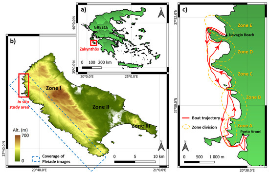
Figure 1.
(a) Location of Zakynthos (Zante) Island in Greece. (b) Spatial coverage of Pléiades satellite images and in situ study area location. (c) Focus on the in situ study area (red square in (b)) with the boat trajectory and the subdivision of the zone used for structure-from-motion processing.
More specifically, the island consists of the following geological formations units. The entire western and north-eastern part of Zakynthos is covered by limestones and dolomites of Late Cretaceous age. In the south-eastern edge of the island, Triassic evaporites are occasionally found. These two formations are the only ones among those expressed superficially that fall into the category of alpine formations. The rest of the island is covered by Neogene and Quaternary sedimentary formations.
More precisely, the central-eastern and south-eastern part of Zakynthos is covered by marine sedimentary formations of Pliocene to Pleistocene age. The central part of the island is covered by Holocene alluvial sediments. The remaining part consists of calcareous marls, limestones and other sedimentary formations of Miocene age [53,54,55,56,57].
Zakynthos has various topographical features. Three geomorphological units (Figure 1b) are distinguished to describe Zakynthos Island (e.g., [58,59,60]):
(i) The Vrachionas mountains are on the western part of the island (see zone I in Figure 1b). This is a mountainous area with generally steep slopes. The steepest slopes (>10%) are found at the eastern boundary of this unit (up to the coastal zone) and decrease westwards [61]. This unit is characterized mainly by limestone formations of the pre-Apulian zone, which is composed of a central karstic plateau and bordered by faulted areas to the east and west. Alluvial cones can be found to the east and deep dissected ravines to the west. Despite this morphological regime, the drainage network is not very well developed. The region is mainly drained by small, ephemeral streams of low drainage density and frequency, but with some deep V-shaped valleys. Most streams have a westward or eastward direction. In the north-western part of the island, the drainage network is relatively well developed compared with the rest of this unit. In this unit, due to this geological and geomorphological configuration, rock falls from coastal cliffs are a major problem [61].
(ii) The fertile central plain (see zone II in Figure 1b) is a faulted basin structure composed of alluvial deposits and sand formations in the coastal region and of Miocene and Pliocene sediments resulting from differential erosion. The morphological slopes are generally less than 2%, but close to the coast, it increases to 2–10% [61].
(iii) The Skopos mountainous peninsula is in the south-eastern part of the island (see zone III in Figure 1b), which is certainly an uplift faulted block, consisting of Ionian limestone, evaporitic rocks, and Pliocene and quaternary deposits [59]. This region also has poor drainage network development but with relatively deep V-shaped valleys flowing westwards and eastwards. The morphological slopes vary from less than to more than 30%. The coastal part also follows the following trend: the western part of this unit (i.e., NW and S coasts) displays high inclinations (10–30%, occasionally up to 42%). The north-central and north-eastern coasts display intermediate inclinations (2–10%) and the eastern coasts display small inclinations (up to 2%) [61].
The in situ study took place in the western coastal part of the Vrachionas mountain. The study area extended from Porto Vromi to Navagio Beach, which represents about 11.2 km of coastline, mainly composed of steep (quasi-vertical) limestone cliffs that can reach 400 m high. From the land, there is no access to the cliff foot, as the cliff face plunges directly into the sea over almost the whole area.
According to [61], the slopes in the coastal area vary from 0 to 30%. More specifically, most of the prominent capes from the central part southwards display an inclination of less than 2%, whereas the intermediate parts display a 20–30% slope. From the center northwards, the capes generally have a 10–20% inclination and the intermediate parts have a slope of 10–30%.
According to the available geological maps [53,54,55,56,57], all of the area of the in situ study is covered by limestones. More specifically, there exist both limestone and dolomitic mudstones and wackstones, with packstone and grainstone interbeddings and, in some locations, radiolitid rudstones and floatstones. The age of these carbonate formations is Turonian to Lower Campanian.
The focus was on the southern areas (zones A, B and C), whereas zone D, with a gentler slope, and the steep Navagio Bay (zone E), were optional. Zone D had the highest elevation in the study area, with a maximum height of approximately 251 m. A description of each zone is available in Figure 2.
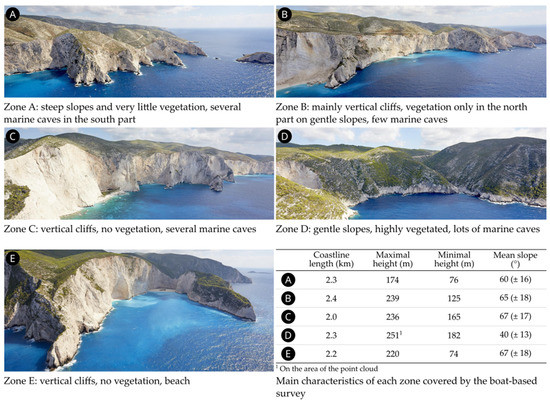
Figure 2.
Description and overview of the 5 studied zones (© 2023 Geotag Aeroview).
Zone B was precisely chosen for the UAS survey after considering several parameters. A field trip along the south-western coast of Zakynthos Island enabled the identification of zone B as a site that combined the following characteristics:
- Visible mass movements;
- An exposure compatible with the satellite acquisition (not too many parts exposed to the north);
- A straight-lined shape;
- A cliff top that was easily accessible so that the UAS could have a departure point from the cliff top;
- Variations in the cliff profile, with various slopes and rock covers.
2.2. Boat-Based Smartphone SfM Photogrammetry
The boat-based SfM photogrammetric survey was performed on the 16 June 2022 using three smartphones (see Table 1), keeping the same orientation during the whole acquisition (Figure A1). Due to the movement of the boat, some photos were blurred or poorly framed and were removed from this count. As far as possible, the operators tried to maintain an image overlap of about 80%. It can be noticed that more photos were required to ensure the same image overlap when the smartphone was kept in portrait mode.

Table 1.
Settings of the smartphone used for the boat-based survey and number of collected photographs.
The trajectory of the boat (see Figure 1c) included two distances for the acquisition: one close to the cliff (from about 50 m to 200 m) on the outward journey and the other farther away on the return journey (about 400–500 m). By varying the distance, the geometry of the camera network could be optimized and rigid body rotation avoided [62]. The survey of 17 km of coastline was performed in about 1 h from a boat (5 m long) with wave conditions between 0.5 m and 1 m.
To improve the consistency of the positions measured by the internal global navigation satellite system (GNSS) receivers, only the geotags of the images captured with the Wiko Smartphone (and the GPS Map Camera app in optimized positioning mode) were used. The boat trajectory was also recorded using the internal GNSS receiver of the Wiko Smartphone. All the images were processed using one chunk in Agisoft Metashape®.
Capes and points are often associated with lower cliffs and less steep slopes. In addition, these areas are more complicated to reconstruct using photogrammetry because of the high overlap required to capture the abrupt variations in orientation. In this study, we therefore focused on 11.2 km of coastline, more precisely on the coves and bays (hence the division into zones, as shown in Figure 1c). For reasons of computing capacity, we processed these different zones separately. The SfM processing was carried out with the Agisoft Metashape® software (version 2.0.1 build 15986—64 bit) using only the geotag of the photos acquired using the Wiko smartphone. For each zone, a 3D RGB point cloud was exported. Locally, when the point cloud appeared noisy, it was filtered manually.
A similar survey could have been carried out using a DSLR camera equipped with GPS geolocation, taking care to maintain a large overlap between the images. This would have also avoided blurred images.
2.3. Pléiades Satellite Imagery
The Pléiades satellites (1A and 1B) were launched by the French Spatial Agency (CNES) and are operated by Airbus DS. Launched in 2011 and 2012, they provide very high-resolution (VHR) optical imagery (a native ground sampling distance of 0.70 m in panchromatic mode), with a daily revisit capability and the ability to acquire off-axis images (up to 40° from the nadir).
For this study, we ordered tri-stereo Pléiades imagery thanks to the HIRACLES (High-Resolution Imagery for Cliff Erosion Studies) project, which is supported by the French Space Agency (CNES). The ordered images had a high angle of incidence (see Table 2) to have a better view of the cliff face and to be able to reconstruct it with a high enough point density [63]. The images, captured on the 17 June 2022, covered approximately 185 km2, corresponding to about 74 km of coastline (Figure 1b), with a cloud coverage of less than 0.7%.
Table 2.
Settings of the tri-stereo Pléiades acquisition used for the satellite 3D reconstruction comparison.
The tri-stereo panchromatic images were processed using Agisoft Metashape®, as proposed in [64]. Given the verticality of the object of study, the digital surface model (DSM) and the orthophotograph were of poor interest; therefore, a 3D grey-level point cloud was exported.
2.4. UAS SfM Photogrammetry
UAS SfM photogrammetry is now a widely used method for 3D reconstructions [38], including for cliff face monitoring [16,33,65,66].
The flight plan to monitor a cliff face was difficult to design. To optimize the flight and to take pictures of the cliff rather than the sea, the UAS had to fly backwards while maintaining a good trade-off between the viewing angle, limiting occlusion effects, spatial resolution on the cliff face and flight safety (flying too close to the cliff face exposes the UAS to local wind effects and loss of GPS signal).
For this study, the UAS survey was performed using a DJI Phantom 4 Pro RTK equipped with a CMOS 1″ sensor (20 MP) to cover zone B. A double-gridded flight plan method (Figure 3a) was used with a constant height. This flight plan was designed with crossed s-shaped paths to create a 3D model. The pitch angle could be set between −90° (downwards) and 30° (0° being forwards) to adjust the acquisition with vertical cliffs. The flight was set up at 35 m above the flight departure point (located on the cliff top) with a mean incidence angle (pitch) of 72.5° (from nadir) and an overlap of 60% (see Table 3).
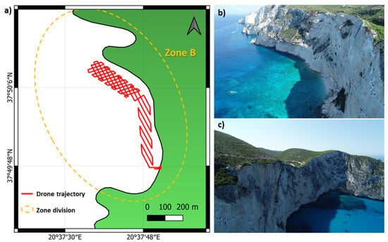
Figure 3.
(a) UAS flight plan used for the zone B survey. (b) UAS photograph of the northern part of zone B with vegetation in the background and a visible rockfall in the foreground. (c) UAS photograph of the southern part of zone B with steep slopes and vegetation.
Table 3.
Mean settings of the UAS survey flight plan.
2.5. Inter-Comparison Method
The inter-comparison was performed with CloudCompare, which is a free 3D point cloud (and triangular mesh) processing software (2.12.4 version). Figure A2 shows some image samples from all the sensors used for this study, prior to processing.
Absolute georeferencing of Pléiades imagery and Smartphone geotagging is accurate to the order of one to a few metres. Therefore, we decided to make relative comparisons by aligning the clouds with each other in each zone. For this inter-comparison, as a lower point density was expected for the stereo-satellite point cloud, these data were meshed (with a maximum edge length of 5 m). The boat-based Smartphone SfM point cloud was registered with the Pléiades mesh using the “Iterative Closest Point” method (ICP) proposed in CloudCompare®. Both datasets were cropped to the same area. Finally, the boat-based smartphone SfM point cloud was compared with the mesh by calculating the absolute distances for all points in the cloud with a cloud-to-mesh approach (C2M).
Some areas were masked (due to obstruction) in the satellite acquisition, which could cause a lack of data in the satellite point cloud and in the subsequent mesh. For the areas corresponding to such an absence of data, a bias in the distance calculation appeared for the points of the smartphone SfM cloud (the distance to the satellite data being necessarily maximized). To limit the biases in the distance calculation, we defined “evaluation zones”, which are extracted from the Pléiades point cloud with a point density higher than 1 point/m2 in a neighbourhood of 10 m2. Absolute distances were also calculated for these “evaluation zones”.
3. Results
3.1. Smartphone SfM Photogrammetry from the Boat
The point clouds generated by Smartphone SfM photogrammetry from the boat covered 7,316,490 m2 of coastal cliff face and showed high point densities ranging from 6.50 points/m2 to 44.13 points/m2 (Table 4). Examples of these point clouds can be viewed in natural colours via the internet link https://youtu.be/HsafwL6yt2o (accessed on 29 June 2022) and in Figure 4a. Locally, some clouds were noisy. This noise, which was removed during processing, generally corresponded to shaded areas of the cliff face (Figure 4b).
Table 4.
Comparison of the resulting point clouds.
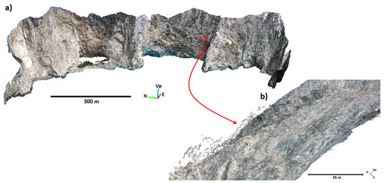
Figure 4.
(a) Point cloud in natural colours generated using SfM photogrammetry from the boat-based smartphone dataset for zone C. (b) Focus on a noisy area in the point cloud.
3.2. Pléiades Satellite Stereorestitution
A grey-level point cloud was derived from Pléiades panchromatic images (Figure 5a) (to keep the finest resolution) using stereo-restitution. A total of 74 km of coastline was reconstructed, as well as the inland areas. For this study, we only focused on the cliff face of zones A to E defined for SfM photogrammetry from a boat. The mean point cloud density on the cliff face varied locally and from one zone to another, ranging from 0.171 points/m2 (zone C) to 0.601 points/m2 (zone D) (see Table 4).
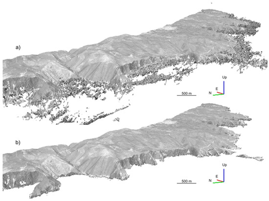
Figure 5.
Stereorestitution of the north-western coast of Zakynthos Island from Pléiades tri-stereo imagery (17 June 2022): (a) before filtering and (b) after filtering on the sea.
The areas corresponding to the sea (with effects related to waves and sun-glint reflection over the water [67,68]) were reconstructed in a very noisy way and interfered with the visualization of the cliff face (Figure 5b). Therefore, these noisy areas needed to be manually filtered from the point cloud first. When filtering, parts of the cliff foot could have been removed along with the noise. The cliff foot was also impacted by tidal effects (of the order of about 20 cm in this area). The boundary of the cliff foot with the Pléiades reconstruction was, therefore, questionable.
Furthermore, the Pléiades point cloud also has missing data, which was caused by occlusions related to a non-optimal configuration between the satellite position, orientation and slope of the cliff face (Figure 6a). Areas that were in steep-sided bays (such as zone E), under an overhang or facing south were particularly affected by these occlusions (Figure 6b).
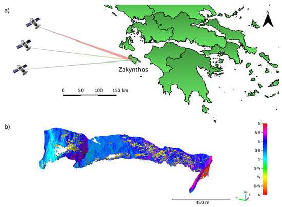
Figure 6.
(a) Position and orientation of the Pléiades satellites with respect to the western coast of Zakynthos during the acquisition of the image triplet on 17 June 2022. (b) Example of the variations of cliff face orientations in zone B.
3.3. UAS SfM Photogrammetry
The UAS flight provided an RGB reconstruction of the cliff on 1.4 km of coastline with a point cloud density of 12.5 points/m2 and a mean camera location error of 0.22 m. The occlusions that were visible in Figure 7 were related to areas not covered by the flight plan (see Figure 3). The cliff face appeared dark on the reconstruction because the flights were made in the morning and the cliff was in shadow.
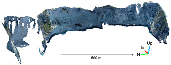
Figure 7.
Three-dimensional reconstruction of the Porto Vromi coast in Zakynthos Island from the UAS survey (zone B).
3.4. Inter-Comparison
We carried out qualitative and quantitative inter-comparisons on the zones common to the different survey methods. Only zone B was covered by all three methods (Pléiades tri-stereo, UAS SfM photogrammetry and SfM photogrammetry from the boat).
Table 4 summarizes the mean distances and standard deviations obtained for these different comparisons and Figure 8 and Figure 9 show the spatial distribution of these differences. For a given zone, the area covered by the different methods was broadly similar (Table 4). In terms of the point density, the SfM photogrammetry from the UAS and from the boat were of the same order of magnitude and had a density about 200 times higher than the Pléiades reconstruction (Table 4). As expected, the configuration with gentle slopes was the most favourable for Pléiades stereorestitution and the least favourable for SfM from the boat. Indeed, the more normal the viewing axis was to the imaged surface, the better the point density (and the fewer obstructions).
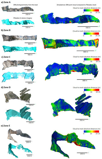
Figure 8.
Three-dimensional reconstructions with the smartphone SfM photogrammetric survey from a boat and with Pléiades tri-stereo imagery (left). Absolute distance comparison between smartphone SfM point cloud and Pléiades mesh (right) for (a) zone A, (b) zone B, (c) zone C, (d) zone D and (e) zone E.
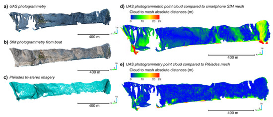
Figure 9.
Three-dimensional reconstructions with the (a) UAS SfM photogrammetric survey, (b) smartphone SfM photogrammetric survey from a boat and (c) Pléiades tri-stereo imagery (left). Absolute distance comparison of the UAS SfM photogrammetric point cloud with a (d) smartphone SfM point cloud and (e) Pléiades mesh (right) for zone B.
Regarding the geometric quality of the reconstructions, it was difficult to define a reference model. Indeed, each method was potentially affected by errors from different origins. By aligning the point clouds with respect to each other, the geolocation error was eliminated and only the error purely related to the 3D reconstruction was considered.
Figure 8 shows recurring gaps in all areas where sea caves were present at the cliff foot. Indeed, given the acquisition geometry, these caves were very easily visible using photogrammetry from the boat, whereas they were difficult to image with Pléiades imagery. Ignoring obstructions (such as sea caves) and focusing on the assessment area, the average difference between the Pléiades point cloud and boat-based photogrammetry was about 2 m for zones A, C, D and E.
In zone B, the difference between the Pléiades and boat-based photogrammetry was higher (4.91 m average difference and 4.50 m standard deviation). Zone B was particularly complex because it had a variety of slopes, textures (bare rock, vegetation cover on gentle slopes, etc.) and orientations (Figure 6b), and therefore, a variety of illuminations. Zone B was also the zone with the longest survey line, which caused a greater distortion at the survey boundaries compared with the other zones.
Zone B had an additional UAS survey, allowing for a more complete inter-comparison (Figure 8b and Figure 9). The UAS/Pléiades comparison gave a mean deviation of 2.47 m (standard deviation of 6.36 m), which was of the same order of magnitude as the boat/Pléiades comparisons over zones A, C, D and E. The mean difference between the UAS/boat point clouds was 6.02 m (standard deviation 8.50 m).
The inter-comparison of zone B showed that the point cloud from the smartphone SfM photogrammetry by boat and the point cloud acquired using the UAS had a larger absolute distance at the edges of the surveys (Figure 9d). The point cloud acquired using the UAS was consistent with the stereorestitution from the Pléiades images, with a homogeneous and constant absolute distance (Figure 9e).
Four cross sections of zone B were extracted from the three point clouds (boat-based, Pléiades and UAS) (Figure 10). The boat-based and the UAS SfM point clouds were both close to the Pléiades 3D reconstruction. The main differences were at the cliff foot. The Pléiades point cloud had few points as it approached closer to the cliff foot. The boat-based and UAS SfM point clouds showed homogeneous point densities, even at the cliff foot.
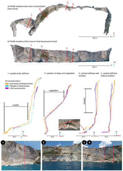
Figure 10.
Comparison of the 3D reconstruction from the smartphone SfM photogrammetric survey, Pléiades tri-stereo imagery and UAS survey, with various ground covers and slopes: (a) top view of the profile locations and (b) front view of the profile locations. Four profiles are presented: (1) case of a rockfall at the cliff foot (image from © Jaud), (2) case of a slope variation and vegetation cover (image from © Jaud), (3) case of a vertical cliff with shadows (image from © Jaud) and (4) case of a vertical cliff without shadow (image from © Jaud).
An inter-comparison was also conducted for zone B to identify the possible impact of ground cover and/or slope on the quality of the reconstruction. X- and Z-shifts were observed between the smartphone SfM point cloud and the UAS SfM and Pléiades tri-stereo point clouds. The X-shift at the edges of the point cloud was the result of geometric distortions. The UAS SfM and Pléiades tri-stereo point clouds had the same behaviour over vegetation and shadow areas. A Z-shift was visible in Figure 10(1) over the rockfall area between the UAS SfM and Pléiades point clouds. An overall consistency between the Pleiades and UAS point clouds was observed above 36 m from the cliff foot. While showing the impact of the acquisition geometry from the boat, with a distortion of the cliff face vertically, Figure 10 shows no obvious impact of ground cover like vegetation or the slope (Figure 10(2)) on the 3D reconstruction for the three acquisition methods. The 3D reconstruction of a boulder at the cliff foot, which resulted from a rockfall, appears in Figure 10(3) in the point cloud from the boat-based survey. A zoomed image of this boulder is shown in Figure 10. Only slight noise was observed in the near shadow areas and for vertical cliffs (and thus steep slopes) on the Pléiades point cloud (Figure 10(3,4)).
4. Discussion
4.1. Advantages and Drawbacks of Each Method
The three survey methods varied mainly in their acquisition geometry. While Pléiades imagery offered the visibility of several kilometres of coastline with few distortions, it could not provide a great view of overhanging parts of the cliff. Objects exposed to the north were also challenging for satellite acquisition, which could be a constraint for some study areas. In addition, acquisitions must be programmed with complex off-nadir angles and a clear sky, with no clouds hiding the cliff face. This approach allowed for identification of rockfalls and cliff variations down to 2 m (Table 5). In this study area, sea caves called “blue caves” could be found at the cliff foot. These parts (which corresponded to 10% of the studied coastline) could not be reconstructed using Pléiades images, thus erosion and rockfall deposits could be missed. This was a strength of boat-based photogrammetric survey. Given its camera positions along the cliff foot, the boat approach enabled enough qualitative VHR images of the cliff foot, including the blue caves, to reconstruct these parts of the cliff. The downside of the boat-based method was the difficulty in imaging the parts above overhangs. Wave conditions must be low to avoid the blurring of the photographs, though using high-quality cameras with a fast shutter speed lens could avoid this issue. Furthermore, lacking RTK positioning, photogrammetric processing was not sufficiently constrained and generated geometric distortions in the model. These distortions corresponded to a “bowl effect” (or “doming effect” for the aerial survey) [33,69,70,71], which is a classic phenomenon for pseudo-linear photogrammetry surveys for which there are insufficient constraints on the image network (lack of ground control points and/or precise camera positioning) [72]. A bias of about 2 m at the edges of the survey was observed in our study (Table 5). With these limitations, the quantification of eroded volume was hampered proportionally to the length of the surveyed coastline. Both boat-based and UAS SfM surveys offered a diversity of viewing angles that were suitable for the non-linear coastline. The RTK positioning of the UAS made it possible to constrain the photogrammetric reconstruction, limiting the distortion effects potentially related to the method, and therefore, enabled geometrically reliable point clouds to be generated. Thus, sub-metre rockfalls and cliff variations could be detected. However, the wind must be weak to reduce effects near the cliff face and the UAS’s battery autonomy limited the linear extent that could be surveyed, unlike the boat-based survey or the Pléiades tri-stereo imagery. Consistency between the UAS SfM and Pléiades point clouds was achieved above 36 m from the cliff foot. As this value was correlated with the height of marine caves and rockfall accumulations at the cliff foot, the satellite approach remained effective for studying large coastlines. Note that optical satellite imagery for emergency response and disaster risk management requires a request (e.g., through Copernicus Emergency Management Service [73]) and remains subject to weather conditions (i.e., no clouds).
Table 5.
Advantages and drawbacks of each survey method.
The vegetated areas were reconstructed in quite a similar way for the boat-based and UAS surveys, whereas the Pléiades 3D reconstruction seemed to smooth out these areas, probably due to the lower spatial resolution.
Results can be generalized to other coastal areas with vertical sea cliffs, especially where there is no large reef flat at the cliff foot to conduct a terrestrial (out of the water) survey, and independently of the tide. However, homogeneous luminosity is required during each survey; otherwise, the SfM reconstruction may not match the images correctly.
4.2. Prospects
We have little or no means of improving the quality of the Pléiades reconstruction.
UAS and boat-based SfM surveys seem to complement each other in terms of viewing angles, and are consistent in terms of resolution and acquisition constraints (high overlap between images taken from different viewpoints). Therefore, images collected from both platforms could be combined in a single process. The boat-based images would benefit from the RTK georeferencing of the UAS images, which are complementary. The combination of both methods should enhance the results.
Regarding the boat-based survey with smartphone SfM photogrammetry, at this time no quality indicator is available with geotagged images. Assessing the position of the cameras is thus impossible. Although there is distortion in the boat-based survey, it is only impactful on a large scale. By working on portions equivalent to the size of a rockfall (a few metres of coastline), we can derive a fair estimate of the eroded volumes. A first suggestion would be to detect rockfalls with the distance comparison (C2M) between two boat-based surveys. The georeferencing of the two surveys can then be refined by studying only the part involved in the rockfall (more limited area to reduce bowl effect). Thus, both detection and quantification of rockfalls can be improved. By offering a rapid and inexpensive survey with limited equipment, the boat-based approach increases the repeatability of the measurements. Thus, mass movements can be identified and correlated with triggering factors, processes or seasons. In addition, it allows for a first estimate of the volumes eroded before the debris are evacuated by the tide. We can also obtain, as for the UAS survey, precisely geotagged photographs by pairing the smartphone with an RTK positioning method. The measurement system described in [23] using an RTK GNSS antenna placed on a wooden frame above the camera would improve the geotag positioning. In this way, the smartphone clock is synchronized with the GNSS clock and the RTK precision can be added to the smartphone. Furthermore, for decision-makers, these results can provide initial quantified data to assess the impact of changes in meteorological and marine variables (induced by climate change) on the recession rate of fast-retreating cliffs.
Having an RTK positioning for the boat-based survey and combining UAS survey with the boat-based survey will be investigated in further work.
5. Conclusions
This study showed that very high-resolution remote sensing methods make it possible to observe the cliff face, even when the cliff foot is not accessible. The inter-comparison showed that the mean distances between the point clouds produced by the different methods were about 2 m. With such precision, mainly major cliff mass movements can be observed.
The reconstruction from the Pléiades tri-stereo appeared to be coherent on a large scale, even if it locally suffered from occlusions or a lack of spatial resolution and had a brief acquisition and processing time. Boat-based photogrammetry seemed to be the most suitable method to represent the cliff foot and to model overhanging areas or sea cave entrances. However, the geotag of smartphone photographs was not accurate enough to generate reliable 3D models over long distances. Although the post-processing time increased with the extent of the measured area, this rapid and inexpensive survey provided an order of magnitude of the cliff face evolutions. This information is relevant for the monitoring of scree, which is often a precursor of larger mass movements. The boat-based survey can also be used as a first estimate for risk management services in emergencies. The UAS survey approach has a flexible acquisition geometry that allows for an in between result, with the limitation of flight autonomy. Furthermore, for surveys of a few hundred metres, UAS SfM photogrammetry appears to be the most reliable method since RTK positioning makes it possible to constrain the photogrammetric reconstruction and, therefore, limits the effects of distortions potentially related to the method. Based on the consistency between the UAS SfM and Pléiades point clouds (above the cave and rockfall height), the satellite approach remains the most effective for studying the evolution of coastal cliffs over several hundreds of kilometres.
Author Contributions
Conceptualization, Z.B., M.J. and P.L.; methodology, Z.B., M.J. and P.L.; software, Z.B. and M.J.; validation, Z.B. and M.J.; formal analysis, Z.B., M.J. and P.L.; investigation, Z.B. and M.J.; resources, Z.B., M.J., P.L., E.V. and N.E.; data curation, Z.B. and M.J.; writing—original draft preparation, Z.B. and M.J.; writing—review and editing, Z.B., M.J., P.L., E.V., N.E., S.C. and C.D.; visualization, Z.B. and M.J.; supervision, P.L., M.J., E.V., N.E., S.C. and C.D.; project administration, P.L.; funding acquisition, P.L. All authors have read and agreed to the published version of the manuscript.
Funding
This research was funded by ARED/BreTel with the support of the Bretagne region and the University of Brest and the ISblue project, which is the Interdisciplinary graduate school for the blue planet, grant number ANR-17-EURE-0015) that is co-funded by a grant from the French government under the program “Investissements d’Avenir” embedded in France 2030. This research was also supported by the CNES (HIRACLES project). It is based on observations with Pléiades satellites. This work was also supported by the Scientific Council of the Institut Universitaire Européen de la Mer.
Data Availability Statement
The following video presents the boat-based photogrammetric reconstructions of Zakynthos cliffs: https://www.youtube.com/watch?v=HsafwL6yt2o (accessed on 22 July 2022). The point clouds generated from the boat-based photogrammetric surveys are available with these DOIs: https://doi.org/10.35110/52e34a6d-e062-4932-a26a-95cf9c2c168f (accessed on 22 July 2022); https://doi.org/10.35110/8096f3ed-b536-4767-8e52-55d93efd6235 (accessed on 22 July 2022); https://doi.org/10.35110/2eae67c3-5cd5-463f-9973-04288fc221ad (accessed on 22 July 2022); https://doi.org/10.35110/dd2c29bb-d251-4e5f-bda8-7f5346a80631 (accessed on 22 July 2022); https://doi.org/10.35110/9f656bf6-436a-49fd-b288-3ab63b83854e (accessed on 22 July 2022).
Acknowledgments
The authors would like to thank Maria Tzouxanioti for her assistance during the fieldwork, Aliki Konsolaki for post-processing the UAS raw data and validating the SfM primary results, and Tina Geller for her English proofreading.
Conflicts of Interest
The authors declare no conflict of interest.
Appendix A

Figure A1.
Diagram of the image acquisition configuration for the smartphone survey (image from © Jaud).

Appendix B

Figure A2.
Image samples from the various sensors compared in the study.

References
- Letortu, P.; Le Dantec, N.; Augereau, E.; Costa, S.; Maquaire, O.; Davidson, R.; Fauchard, C.; Antoine, R.; Flahaut, R.; Guirriec, Y.; et al. Experimental field study on the fatigue and failure mechanisms of coastal chalk cliffs: Implementation of a multi-parameter monitoring system (Sainte-Marguerite-sur-Mer, France). Geomorphology 2022, 408, 108211. [Google Scholar] [CrossRef]
- Cooley, S.R.; Schoeman, D.S.; Bopp, L.; Boyd, P.; Donner, S.; Ito, S.-I.; Kiessling, W.; Martinetto, P.; Ojea, E.; Racault, M.-F.; et al. 2022: Oceans and Coastal Ecosystems and Their Services. In Climate Change 2022: Impacts, Adaptation and Vulnerability. Contribution of Working Group II to the Sixth Assessment Report of the Intergovernmental Panel on Climate Change; Pörtner, H.-O., Roberts, D.C., Tignor, M., Poloczanska, K., Mintenbeck, K., Alegría, A., Craig, M., Langsdorf, S., Löschke, S., Möller, V., et al., Eds.; Cambridge University Press: Cambridge, UK, 2022; pp. 379–550. [Google Scholar]
- Bondarenko, M.; Kerr, D.; Sorichetta, A.; Tatem, A. Census/Projection-Disaggregated Gridded Population Datasets for 189 Countries in 2020 Using Built-Settlement Growth Model (BSGM) Outputs; University of Southampton: Southampton, UK, 2020. [Google Scholar]
- Reimann, L.; Vafeidis, A.T.; Honsel, L.E. Population development as a driver of coastal risk: Current trends and future pathways. Camb. Prism. Coast. Futur. 2023, 1, e14. [Google Scholar] [CrossRef]
- Young, A.P.; Carilli, J.E. Global distribution of coastal cliffs. Earth Surf. Process. Landforms 2019, 44, 1309–1316. [Google Scholar] [CrossRef]
- Costa, S. “Dynamique Littorale et Risques Naturels”: L’impact Des Aménagements, Des Variations Du Niveau Marin et Des Modifications Climatiques Entre La Baie de Seine et La Baie de Somme (Haute-Normandie, Picardie; France). Ph.D. Thesis, University of Paris, Paris, France, 1997. [Google Scholar]
- Zviely, D.; Klein, M. Coastal cliff retreat rates at Beit-Yannay, Israel, in the 20th century. Earth Surf. Process. Landforms 2004, 29, 175–184. [Google Scholar] [CrossRef]
- Foyle, A.M.; Naber, M.D. Decade-scale coastal bluff retreat from LiDAR data: Lake Erie coast of NW Pennsylvania, USA. Environ. Earth Sci. 2012, 66, 1999–2012. [Google Scholar] [CrossRef]
- Letortu, P.; Taouki, R.; Jaud, M.; Costa, S.; Maquaire, O.; Delacourt, C. Three-dimensional (3D) reconstructions of the coastal cliff face in Normandy (France) based on oblique Pléiades imagery: Assessment of Ames Stereo Pipeline® (ASP®) and MicMac® processing chains. Int. J. Remote. Sens. 2021, 42, 4558–4578. [Google Scholar] [CrossRef]
- Terefenko, P.; Paprotny, D.; Giza, A.; Morales-Nápoles, O.; Kubicki, A.; Walczakiewicz, S. Monitoring Cliff Erosion with LiDAR Surveys and Bayesian Network-based Data Analysis. Remote Sens. 2019, 11, 843. [Google Scholar] [CrossRef]
- Terefenko, P.; Wziątek, D.Z.; Dalyot, S.; Boski, T.; Lima-Filho, F.P. A High-Precision LiDAR-Based Method for Surveying and Classifying Coastal Notches. ISPRS Int. J. Geo-Inf. 2018, 7, 295. [Google Scholar] [CrossRef]
- Swirad, Z.M.; Young, A.P. Automating coastal cliff erosion measurements from large-area LiDAR datasets in California, USA. Geomorphology 2021, 389, 107799. [Google Scholar] [CrossRef]
- Young, A.P.; Olsen, M.J.; Driscoll, N.; Flick, R.; Gutierrez, R.; Guza, R.; Johnstone, E.; Kuester, F. Comparison of Airborne and Terrestrial Lidar Estimates of Seacliff Erosion in Southern California. Photogramm. Eng. Remote. Sens. 2010, 76, 421–427. [Google Scholar] [CrossRef]
- Vassilakis, E.; Konsolaki, A.; Petrakis, S.; Kotsi, E.; Fillis, C.; Triantaphyllou, M.; Antonarakou, A.; Lekkas, E. Combination of Close-Range Remote Sensing Data (TLS and UAS) and Techniques for Structural Measurements across the Deformation Zone of the Ionian Thrust in Zakynthos Isl. In Proceedings of the 16th International Congress of the Geological Society of Greece, Patras, Greece, 17–19 October 2022. [Google Scholar]
- Diakakis, M.; Vassilakis, E.; Mavroulis, S.; Konsolaki, A.; Kaviris, G.; Kotsi, E.; Kapetanidis, V.; Sakkas, V.; Alexopoulos, J.D.; Lekkas, E.; et al. An Integrated UAS and TLS Approach for Monitoring Coastal Scarps and Mass Movement Phenomena. The Case of Ionian Islands. In Proceedings of the EGU General Assembly 2022, Vienna, Austria, 23–27 May 2022. [Google Scholar]
- Gallo, I.G.; Martínez-Corbella, M.; Sarro, R.; Iovine, G.; López-Vinielles, J.; Hérnandez, M.; Robustelli, G.; Mateos, R.M.; García-Davalillo, J.C. An Integration of UAV-Based Photogrammetry and 3D Modelling for Rockfall Hazard Assessment: The Cárcavos Case in 2018 (Spain). Remote. Sens. 2021, 13, 3450. [Google Scholar] [CrossRef]
- Karantanellis, E.; Marinos, V.; Vassilakis, E.; Christaras, B. Object-Based Analysis Using Unmanned Aerial Vehicles (UAVs) for Site-Specific Landslide Assessment. Remote. Sens. 2020, 12, 1711. [Google Scholar] [CrossRef]
- Brush, J.A.; Pavlis, T.L.; Hurtado, J.M.; Mason, K.A.; Knott, J.R.; Williams, K.E. Evaluation of field methods for 3-D mapping and 3-D visualization of complex metamorphic structure using multiview stereo terrain models from ground-based photography. Geosphere 2018, 15, 188–221. [Google Scholar] [CrossRef]
- Hansman, R.J.; Ring, U. Workflow: From photo-based 3-D reconstruction of remotely piloted aircraft images to a 3-D geological model. Geosphere 2019, 15, 1393–1408. [Google Scholar] [CrossRef]
- Vanneschi, C.; Di Camillo, M.; Aiello, E.; Bonciani, F.; Salvini, R. SfM-MVS Photogrammetry for Rockfall Analysis and Hazard Assessment Along the Ancient Roman Via Flaminia Road at the Furlo Gorge (Italy). ISPRS Int. J. Geo-Inf. 2019, 8, 325. [Google Scholar] [CrossRef]
- Gonçalves, G.; Gonçalves, D.; Gómez-Gutiérrez, A.; Andriolo, U.; Pérez-Alvárez, J.A. 3D Reconstruction of Coastal Cliffs from Fixed-Wing and Multi-Rotor UAS: Impact of SfM-MVS Processing Parameters, Image Redundancy and Acquisition Geometry. Remote. Sens. 2021, 13, 1222. [Google Scholar] [CrossRef]
- Genchi, S.A.; Vitale, A.J.; Perillo, G.M.E.; Delrieux, C.A. Structure-from-Motion Approach for Characterization of Bioerosion Patterns Using UAV Imagery. Sensors 2015, 15, 3593–3609. [Google Scholar] [CrossRef]
- Jaud, M.; Bertin, S.; Beauverger, M.; Augereau, E.; Delacourt, C. RTK GNSS-Assisted Terrestrial SfM Photogrammetry without GCP: Application to Coastal Morphodynamics Monitoring. Remote. Sens. 2020, 12, 1889. [Google Scholar] [CrossRef]
- Tavani, S.; Pignalosa, A.; Corradetti, A.; Mercuri, M.; Smeraglia, L.; Riccardi, U.; Seers, T.; Pavlis, T.; Billi, A. Photogrammetric 3D Model via Smartphone GNSS Sensor: Workflow, Error Estimate, and Best Practices. Remote. Sens. 2020, 12, 3616. [Google Scholar] [CrossRef]
- Tavani, S.; Granado, P.; Riccardi, U.; Seers, T.; Corradetti, A. Terrestrial SfM-MVS photogrammetry from smartphone sensors. Geomorphology 2020, 367, 107318. [Google Scholar] [CrossRef]
- Micheletti, N.; Chandler, J.H.; Lane, S.N. Investigating the geomorphological potential of freely available and accessible structure-from-motion photogrammetry using a smartphone. Earth Surf. Process. Landforms 2015, 40, 473–486. [Google Scholar] [CrossRef]
- Sofia, G.; Masin, R.; Tarolli, P. Prospects for crowdsourced information on the geomorphic ‘engineering’ by the invasive Coypu (Myocastor coypus). Earth Surf. Process. Landforms 2017, 42, 365–377. [Google Scholar] [CrossRef]
- Corradetti, A.; Seers, T.; Mercuri, M.; Calligaris, C.; Busetti, A.; Zini, L. Benchmarking Different SfM-MVS Photogrammetric and iOS LiDAR Acquisition Methods for the Digital Preservation of a Short-Lived Excavation: A Case Study from an Area of Sinkhole Related Subsidence. Remote. Sens. 2022, 14, 5187. [Google Scholar] [CrossRef]
- Fang, K.; An, P.; Tang, H.; Tu, J.; Jia, S.; Miao, M.; Dong, A. Application of a multi-smartphone measurement system in slope model tests. Eng. Geol. 2021, 295, 106424. [Google Scholar] [CrossRef]
- Luetzenburg, G.; Kroon, A.; Bjørk, A.A. Evaluation of the Apple iPhone 12 Pro LiDAR for an Application in Geosciences. Sci. Rep. 2021, 11, 22221. [Google Scholar] [CrossRef] [PubMed]
- Letortu, P.; Jaud, M.; Grandjean, P.; Ammann, J.; Costa, S.; Maquaire, O.; Davidson, R.; Le Dantec, N.; Delacourt, C. Examining high-resolution survey methods for monitoring cliff erosion at an operational scale. GIScience Remote. Sens. 2018, 55, 457–476. [Google Scholar] [CrossRef]
- Ružić, I.; Marović, I.; Benac, C.; Ilić, S. Coastal cliff geometry derived from structure-from-motion photogrammetry at Stara Baška, Krk Island, Croatia. Geo-Marine Lett. 2014, 34, 555–565. [Google Scholar] [CrossRef]
- Jaud, M.; Letortu, P.; Théry, C.; Grandjean, P.; Costa, S.; Maquaire, O.; Davidson, R.; Le Dantec, N. UAV survey of a coastal cliff face—Selection of the best imaging angle. Measurement 2019, 139, 10–20. [Google Scholar] [CrossRef]
- Jaud, M.; Tscf, I.U.; Rouveure, R.; Moiroux-Arvis, L.; Faure, P.; Monod, M.-O. Boat-borne radar mapping versus aerial photogrammetry and mobile laser scanning applied to river gorge monitoring. Open J. Remote. Sens. Position. 2014, 1, 48–63. [Google Scholar] [CrossRef][Green Version]
- Alho, P.; Kukko, A.; Hyyppä, H.; Kaartinen, H.; Hyyppä, J.; Jaakkola, A. Application of boat-based laser scanning for river survey. Earth Surf. Process. Landforms 2009, 34, 1831–1838. [Google Scholar] [CrossRef]
- Schneider, D.; Blaskow, R. Boat-Based Mobile Laser Scanning For Shoreline Monitoring of Large Lakes. ISPRS Int. Arch. Photogramm. Remote. Sens. Spat. Inf. Sci. 2021, XLIII-B2-2, 759–762. [Google Scholar] [CrossRef]
- Giuliano, J.; Dewez, T.J.B.; Lebourg, T.; Godard, V.; Prémaillon, M.; Marçot, N. Mapping Coastal Erosion of a Mediterranean Cliff with a Boat-Borne Laser Scanner: Performance, Processing, and Cliff Erosion Rate. In 3D Digital Geological Models; Bistacchi, A., Massironi, M., Viseur, S., Eds.; John Wiley & Sons, Ltd.: Hoboken, NJ, USA, 2022; pp. 109–132. ISBN 978-1-119-31392-2. [Google Scholar]
- Westoby, M.; Brasington, J.; Glasser, N.F.; Hambrey, M.J.; Reynolds, J.M. ‘Structure-from-Motion’ photogrammetry: A low-cost, effective tool for geoscience applications. Geomorphology 2012, 179, 300–314. [Google Scholar] [CrossRef]
- Kotsi, E.; Vassilakis, E.; Diakakis, M.; Mavroulis, S.; Konsolaki, A.; Filis, C.; Lozios, S.; Lekkas, E. Using UAS-Aided Photogrammetry to Monitor and Quantify the Geomorphic Effects of Extreme Weather Events in Tectonically Active Mass Waste-Prone Areas: The Case of Medicane Ianos. Appl. Sci. 2023, 13, 812. [Google Scholar] [CrossRef]
- Panagiotopoulou, S.; Erkeki, A.; Antonakakis, A.; Grigorakakis, P.; Protopapa, V.; Tsiostas, G.; Vlachou, K.; Vassilakis, E. Evaluation of Network Real Time Kinematics Contribution to the Accuracy/Productivity Ratio for UAS-SfM Photogrammetry. In Proceedings of the 2020 European Navigation Conference (ENC), Dresden, Germany, 23–24 November 2020; pp. 1–11. [Google Scholar]
- Esposito, G.; Salvini, R.; Matano, F.; Sacchi, M.; Danzi, M.; Somma, R.; Troise, C. Multitemporal monitoring of a coastal landslide through SfM-derived point cloud comparison. Photogramm. Rec. 2017, 32, 459–479. [Google Scholar] [CrossRef]
- Drymoni, K.; Bonali, F.L.; Browning, J.; Gudmundsson, A.; Fallati, L.; Antoniou, V.; Nomikou, P. Field Analysis Vs Boat-Based Photogrammetry Derived Data in Volcanotectonics: An Example from the Santorini Dyke Swarm. In Proceedings of the EGU General Assembly 2020, Copernicus Meetings, Online, 3–8 May 2020. [Google Scholar]
- Jin, D.; Li, J.; Gong, J.; Li, Y.; Zhao, Z.; Li, Y.; Li, D.; Yu, K.; Wang, S. Shipborne Mobile Photogrammetry for 3D Mapping and Landslide Detection of the Water-Level Fluctuation Zone in the Three Gorges Reservoir Area, China. Remote. Sens. 2021, 13, 1007. [Google Scholar] [CrossRef]
- Li, Y.; Wang, P.; Feng, Q.; Ji, X.; Jin, D.; Gong, J. Landslide detection based on shipborne images and deep learning models: A case study in the Three Gorges Reservoir Area in China. Landslides 2023, 20, 547–558. [Google Scholar] [CrossRef]
- Cliff Collapse on Greece’s “shipwreck Beach” Injures Tourists. BBC News, 13 September 2018.
- McKenzie, D. Active tectonics of the Alpine--Himalayan belt: The Aegean Sea and surrounding regions. Geophys. J. Int. 1978, 55, 217–254. [Google Scholar] [CrossRef]
- Le Pichon, X.; Angelier, J. The hellenic arc and trench system: A key to the neotectonic evolution of the eastern mediterranean area. Tectonophysics 1979, 60, 1–42. [Google Scholar] [CrossRef]
- Papanikolaou, M.; Triantaphyllou, M. Post- alpine late pliocene—Middle pleistocene uplifted marine sequences in zakynthos island. Bull. Geol. Soc. Greece 2010, 43, 475–485. [Google Scholar] [CrossRef][Green Version]
- Stiros, S.C.; Pirazzoli, P.A.; Laborel, J.; Laborel-Deguen, F. The 1953 earthquake in Cephalonia (Western Hellenic Arc): Coastal uplift and halotectonic faulting. Geophys. J. Int. 1994, 117, 834–849. [Google Scholar] [CrossRef]
- Zampazas, G.; Karymbalis, E.; Chalkias, C. Assessment of the sensitivity of Zakynthos Island (Ionian Sea, Western Greece) to climate change-induced coastal hazards. Z. Geomorphol. 2022, 63, 183–200. [Google Scholar] [CrossRef]
- Vassilakis, E.; Royden, L.; Papanikolaou, D. Kinematic links between subduction along the Hellenic trench and extension in the Gulf of Corinth, Greece: A multidisciplinary analysis. Earth Planet. Sci. Lett. 2011, 303, 108–120. [Google Scholar] [CrossRef]
- Aubouin, J.; Dercourt, J. Zone preapulienne, zone ionienne et zone du Gavrovo en Peloponnese occidental. BSGF Earth Sci. Bull. 1962, S7-IV, 785–794. [Google Scholar] [CrossRef]
- Underhill, J.R. Triassic evaporites and Plio-Quaternary diapirism in western Greece. J. Geol. Soc. 1988, 145, 269–282. [Google Scholar] [CrossRef]
- Accordi, G.; Carbone, F.; Civitelli, G.; Corda, L.; de Rita, D.; Esu, D.; Funiciello, R.; Kotsakis, T.; Mariotti, G.; Sposato, A. Carta Delle Litofacies Del Lazio-Abruzzo Ed Aree Limitrofe e Note Illustrative. La Ric. Sci. 1988, 5, 114. [Google Scholar]
- Papadopoulos, P. Geological Map of Greece, Scale 1: 50 000 Sheet Maronia; Institute of Geology and Mineral Exploration (IGME): Xanthi, Greece, 1980. [Google Scholar]
- Underhill, J.R. Late Cenozoic deformation of the Hellenide foreland, western Greece. GSA Bull. 1989, 101, 613–634. [Google Scholar] [CrossRef]
- Zelilidis; Kontopoulos; Avramidis; Piper. Tectonic and sedimentological evolution of the Pliocene–Quaternary basins of Zakynthos island, Greece: Case study of the transition from compressional to extensional tectonics. Basin Res. 1998, 10, 393–408. [Google Scholar] [CrossRef]
- Muller-Miny, H. Beitrge Zur Morphologie Und Geologie Der Mittleren Ionischen Inseln Beobachtungen Auf Kephallinia Und Zakynthos. Ann. Geol. Pays Hellen 1965, 16, 178–187. [Google Scholar]
- Gournellos, T.; Vassilopoulos, A.; Evelpidou, N. Development of a GIS-Based Methodology to Analyze Geological, Geomorphological and Environmental Data of the Island of Zakynthos. In Proceedings of the International Symposium on Engineering Geology and the Environment, Athens, Greece, 23–27 June 1997; pp. 1245–1251. [Google Scholar]
- Livaditis, G.; Alexouli, A. Geomorphological Observations in the Island of Zakynthos. In Proceedings of the 3rd Congress of Geographical Society of Greece, Thessaloniki, Greece, 18–21 May 1993. [Google Scholar]
- Gournelos, T.; Evelpidou, N.; Vasilopoulos, A. A Morphometric Analysis Using GIS to Deduce Geomorphological Processes–Natural Hazards at Zakynthos Island. In Proceedings of the 6th International Conference on Environmental Science and Technology, Samos, Greece, 30 August–2 September 1999. [Google Scholar]
- Jaud, M.; Passot, S.; Allemand, P.; Le Dantec, N.; Grandjean, P.; Delacourt, C. Suggestions to Limit Geometric Distortions in the Reconstruction of Linear Coastal Landforms by SfM Photogrammetry with PhotoScan® and MicMac® for UAV Surveys with Restricted GCPs Pattern. Drones 2019, 3, 2. [Google Scholar] [CrossRef]
- Letortu, P.; Jaud, M.; Théry, C.; Nabucet, J.; Taouki, R.; Passot, S.; Augereau, E. The potential of Pléiades images with high angle of incidence for reconstructing the coastal cliff face in Normandy (France). Int. J. Appl. Earth Obs. Geoinf. 2020, 84, 101976. [Google Scholar] [CrossRef]
- Lastilla, L.; Ravanelli, R.; Crespi, M. First Test of Agisoft Metashape Satellite Image Processing for DSM Generation: A Case Study in Trento with Pléiades Imagery. In Proceedings of the IGARSS 2020—2020 IEEE International Geoscience and Remote Sensing Symposium, Waikoloa, HI, USA, 26 September–2 October 2020; pp. 897–900. [Google Scholar] [CrossRef]
- Mancini, F.; Castagnetti, C.; Rossi, P.; Dubbini, M.; Fazio, N.L.; Perrotti, M.; Lollino, P. An Integrated Procedure to Assess the Stability of Coastal Rocky Cliffs: From UAV Close-Range Photogrammetry to Geomechanical Finite Element Modeling. Remote Sens. 2017, 9, 1235. [Google Scholar] [CrossRef]
- Agüera-Vega, F.; Carvajal-Ramírez, F.; Martínez-Carricondo, P.; Sánchez-Hermosilla López, J.; Mesas-Carrascosa, F.J.; García-Ferrer, A.; Pérez-Porras, F.J. Reconstruction of extreme topography from UAV structure from motion photogrammetry. Measurement 2018, 121, 127–128. [Google Scholar] [CrossRef]
- Casella, E.; Collin, A.; Harris, D.; Ferse, S.; Bejarano, S.; Parravicini, V.; Hench, J.L.; Rovere, A. Mapping coral reefs using consumer-grade drones and structure from motion photogrammetry techniques. Coral Reefs 2017, 36, 269–275. [Google Scholar] [CrossRef]
- Partama, I.Y.; Kanno, A.; Ueda, M.; Akamatsu, Y.; Inui, R.; Sekine, M.; Yamamoto, K.; Imai, T.; Higuchi, T. Removal of water-surface reflection effects with a temporal minimum filter for UAV-based shallow-water photogrammetry. Earth Surf. Process. Landf. 2018, 43, 2673–2682. [Google Scholar] [CrossRef]
- James, M.R.; Robson, S. Mitigating systematic error in topographic models derived from UAV and ground-based image networks. Earth Surf. Process. Landforms 2014, 39, 1413–1420. [Google Scholar] [CrossRef]
- Wackrow, R.; Chandler, J.H. Minimising systematic error surfaces in digital elevation models using oblique convergent imagery. Photogramm. Rec. 2011, 26, 16–31. [Google Scholar] [CrossRef]
- Eltner, A.; Schneider, D. Analysis of Different Methods for 3D Reconstruction of Natural Surfaces from Parallel-Axes UAV Images. Photogramm. Rec. 2015, 30, 279–299. [Google Scholar] [CrossRef]
- Tournadre, V.; Pierrot-Deseilligny, M.; Faure, P.H. UAV LINEAR PHOTOGRAMMETRY. ISPRS Int. Arch. Photogramm. Remote. Sens. Spat. Inf. Sci. 2015, XL-3/W3, 327–333. [Google Scholar] [CrossRef]
- Copernicus Emergency Management Service. Available online: https://emergency.copernicus.eu/ (accessed on 17 June 2023).


Disclaimer/Publisher’s Note: The statements, opinions and data contained in all publications are solely those of the individual author(s) and contributor(s) and not of MDPI and/or the editor(s). MDPI and/or the editor(s) disclaim responsibility for any injury to people or property resulting from any ideas, methods, instructions or products referred to in the content. |
© 2023 by the authors. Licensee MDPI, Basel, Switzerland. This article is an open access article distributed under the terms and conditions of the Creative Commons Attribution (CC BY) license (https://creativecommons.org/licenses/by/4.0/).