Article

Modeling the Effects of Drivers on PM2.5 in the Yangtze River Delta with Geographically Weighted Random Forest

1
Zhangzhou Institute of Technology, Zhangzhou 363000, China
2
Earth System Science Interdisciplinary Center, University of Maryland, College Park, MD 20740, USA
3
Guangdong Academy of Forestry, Guangzhou 510520, China
*
Author to whom correspondence should be addressed.
Remote Sens. 2023, 15(15), 3826; https://doi.org/10.3390/rs15153826
Submission received: 16 June 2023 / Revised: 27 July 2023 / Accepted: 28 July 2023 / Published: 31 July 2023

Abstract

:
Establishing an efficient PM2.5 prediction model and in-depth knowledge of the relationship between the predictors and PM2.5 in the model are of great significance for preventing and controlling PM2.5 pollution and policy formulation in the Yangtze River Delta (YRD) where there is serious air pollution. In this study, the spatial pattern of PM2.5 concentration in the YRD during 2003–2019 was analyzed by Hot Spot Analysis. We employed five algorithms to train, verify, and test 17 years of data in the YRD, and we explored the drivers of PM2.5 exposure. Our key results demonstrated: (1) High PM2.5 pollution in the YRD was concentrated in the western and northwestern regions and remained stable for 17 years. Compared to 2003, PM2.5 increased by 10–20% in the southeast, southwest, and western regions in 2019. The hot spot for percentage change of PM2.5 was mostly located in the southwest and southeast regions in 2019, while the interannual change showed a changeable spatial distribution pattern. (2) Geographically Weighted Random Forest (GWRF) has great advantages in predicting the presence of PM2.5 in comparison with other models. GWRF not only improves the performance of RF, but also spatializes the interpretation of variables. (3) Climate and human activities are the most important drivers of PM2.5 concentration. Drought, temperature, and temperature difference are the most critical and potentially threatening climatic factors for the increase and expansion of PM2.5 in the YRD. With the warming and drying trend worldwide, this finding can help policymakers better consider these factors for PM2.5 prediction. Moreover, the effect of interference from humans on ecosystems will increase again after COVID-19, leading to a rise in PM2.5 concentration. The strong explanatory power of comprehensive ecological indicators for the distribution of PM2.5 will be a crucial indicator worthy of consideration by decision-making departments.

Graphical Abstract

1. Introduction

Fine particulate matter (PM2.5) in air pollutants enters the upper respiratory tract of the human body and damages the tracheal mucosa, which reduces its efficiency for killing viruses and bacteria and affects its function for resisting harmful substances from entering lung tissue [1]. At the same time, PM2.5 are inclined to attach heavy metal ions [2] and bacteria with viruses [3], so if they undergo continuous transmission or do not settle for a long time, they will help the spread of infectious diseases [4]. Therefore, accurate and reasonable acquisition and forecast of PM2.5 emission is crucial to solving many problems regarding environmental public health.
Over the past decade, China has gradually built 1607 pollutant information collection stations to monitor severely polluted air [5,6]. However, the short period of recorded data, the spatial discontinuity of ground sites [7], the discontinuity caused by equipment failures, and the inconsistency of equipment in different provinces [8] all make the research on large-scale and long-term series face great challenges. The PM2.5 concentration information retrieved from Aerosol Optical Depth (AOD) [9] or top-of-the-atmosphere reflectance (TOAR) data [6], which is obtained by different remote sensing satellite sensors, effectively ensures spatial coverage [10] and is widely used in the study of various types of pollution emissions and ecological fields around the world [3,6,11,12], especially in the estimation of the future spatial distribution of PM2.5 [4].
Modeling PM2.5 involves estimating the missing parts of spatiotemporal data, which is currently the main effort in the field [3,6,8,10], as well as predicting the distribution of concentrations over a given area in the future [4]. Traditional regression models and machine learning (ML) algorithms were the most frequently selected methods in previous research [8,13,14,15]. Simple and multiple linear regressions, such as land-use regression, occurred most frequently in traditional statistical models [14,16,17]. Recently, many scholars have begun to pay attention to the value of random effects in the model and tried to estimate PM2.5 via a linear mixed effect model [13]. Nevertheless, the complex and nonlinear relationships between PM2.5 and environmental drivers have not been fully discussed. An effective way to solve this problem is with a ML algorithm, including different artificial neural networks [4,17,18,19], support vector machines [16], decision trees [5], gradient boosting machines [1,15,18], and random forests (RF) [9,12,20]. In addition to their ability to capture nonlinear relationships, ML techniques are good at environmental sciences data analysis and modeling because of their abilities to compute big data, high-dimensional data, blended data, and missing values compared to traditional physical, chemical, and regression statistics [14]. However, these global approaches ignore the spatial heterogeneity of PM2.5, which will affect research concerning the effects of PM2.5 on ecological security and human health [5,15]. Therefore, some scholars have recently considered adding geographic weight information to the linear regression method [17], geographically weighted regression (GWR) to the mixed-effects model to form a two-stage model [21], and spatiotemporal random forest to establish a spatiotemporal model of PM2.5 [8].
Unlike spatiotemporal random forests, the geographically weighted random forests considered in this study combine the advantages of RF and GWR. In this way, it can not only capture the nonlinear relationships among data, but also explain the local effect of variables, which is valuable for understanding the fundamental process of the relationship between drivers and response variables within a model [22]. Hengl et al. [23] added geopredictors to RF. Afterwards, Georganos et al. [24] combined GWR and RF to truly develop geographically weighted random forests (GWRFs). So far, GWRFs have been mainly applied to ecology, geography, and epidemiology, with limited applications including forest land change prediction and drivers [25], crop yield prediction [26], and spatial distribution of diabetes prevalence [22]. Still, it has not been widely used in environmental science.
Although the better algorithm contributes more to improving the forecast accuracy of model, the choice of predictors should not be ignored. The scientific relationship between explanatory variables and response variables in predictive models is also crucial [27]. Previous research has indicated that population density and GDP, as indicators of human socio-economic development, are frequently used predictors in PM2.5 estimation models [1]. With the steadily growing economy and the relatively stable population level in the past decade, the vigorous implementation of environmental protection policies and systems has dramatically alleviated air pollution in China. It is insufficient to explain the changing trend of PM2.5 only by the changes in population and economy. A report by Kaur et al. [28] found that a combination of multiple geographic and ecological weight information can provide more reliable results compared to a single parameter. Therefore, we recommend that more comprehensive ecological indicators, such as human disturbance indices, should be considered in pollutant modeling. Meanwhile, Hua et al. [29] reported that biomass combustion, which cannot be ignored in PM2.5 pollution, is also an important source. As we all know, there is a synergistic relationship between air pollution and climate factors that strengthen and influence each other [5,27]. Pollutants change the balance of climate development [30]; meanwhile, these climate elements also play a certain obstructive role in the atmospheric diffusion process of pollutants [12]. Among these climatic factors, the most prominent influences include temperature, precipitation, and humidity [17]. Additionally, the role of vegetation in influencing the deposition and diffusion of pollutants by absorbing and trapping fine dust particles and gaseous pollutants also needs to be considered [20,31]. The search for effective predictors is an important preliminary work to help the government formulate effective air quality improvement strategies, determine the best implementation plan, and depict the air pollution process in the key step of virtual simulation scene modeling.
In this study, we employed five modeling methods to simulate the relationship between PM2.5 concentration and environmental factors in the Yangtze River Delta (YRD), using extracted climate factors, human activities and economic indicators, and vegetation factors and biomass combustion factors as predictive variables. The overall goals of this work were the following: (1) to clarify the spatial pattern of PM2.5 pollution and change in the YRD; (2) to determine the optimal prediction model for PM2.5 concentration; (3) to explore the drivers of PM2.5 given by the best model to provide meaningful help for the prediction of regional pollutant concentration in the future and the modeling of virtual simulation scenarios. We believe that establishing a model with reasonable explanatory ability has important theoretical guiding significance for analyzing the causes of regional air pollution and formulating prevention and control measures for relevant departments.

2. Materials and Methods

2.1. Research Area

We chose the Yangtze River Delta (YRD) (118°33′~123°10′E and 28°0′~33°52′N) as the research site (Figure 1). It is an essential economic area with a high population concentration in eastern China. Due to the high degree of economization and urbanization, this district has been enduring bad air pollution for a long time [32]. With the support of a large number of environmental sustainment policies recently, the quality of the regional atmospheric environment has been continuously improved, but PM2.5, as the primary pollutant, is still higher than the threshold (the annual average concentration is 35 μg/m3) set by the World Health Organization (WHO) and presents an irregular spatial and temporal distribution pattern [12]. The slowly decreasing elevation from southwest to northeast and the low mountains scattered around the periphery hinder the spread of pollutants in the YRD [12]. Also, the frequent human activities and the regular subtropical monsoon climate make different land cover and land use patterns appear in the YRD, thereby presenting complex ecosystem types.

2.2. Data Preparation

2.2.1. PM2.5 Raster Data

This study considered the global annual PM2.5 grid in 2003–2020 as the response variable. These data were produced by combining satellite observations of aerosols (tiny particles suspended in the air) with computer models that simulate the movement of these particles in the atmosphere. The satellite observations are obtained from equipment including the Moderate Resolution Imaging Spectroradiometer (MODIS) and the Multi-angle Imaging SpectroRadiometer (MISR). These instruments measure the amount of sunlight reflected by the earth’s surface and atmosphere at different wavelengths, which can be used to estimate the concentration of aerosols in the atmosphere. In addition, based on the global ground database from the WHO, spatial statistical models adjusted the residual PM2.5 bias for each cell in the initial satellite-derived values [33]. The resulting PM2.5 data is a global dataset that provides information on the atmosphere’s concentration and distribution of fine particulate matter. This data has been widely used to monitor air quality [7], track the movement of pollutants [20], and study the health effects of exposure to PM2.5 [11], and it can be accessed from the Atmospheric Composition Analysis Group (ACAG) at the University of Washington [3]. Van Donkelaar et al. [7] confirmed that this data can be easily applied to China. Hammer et al. [33] also confirmed that this data has a good linear trend with the ground observation data in China, especially in the industrial zone in eastern China. Jin et al. [3] confirmed that this data helps to understand the variation of PM2.5 in different regions of China and its impact on population distribution.

2.2.2. Explanatory Variable

Meteorological Variables

Meteorological conditions are the external factors of the air pollution process because the transfer, diffusion, and deposition of pollutants and other processes are associated with climate. Among them, the important indicators of climate change, such as annual average temperature, annual average diurnal temperature range, and drought [34,35], play a crucial role in understanding the spatio-temporal changes of pollutants under climate change [34]. Therefore, we used the monthly mean temperature, diurnal temperature range, precipitation, and potential evapotranspiration data during 2003–2020 provided by the Climatic Research Unit gridded Time Series (CRU TS) as climate-independent variables in this study. CRU TS is a well-recognized meteorological dataset produced by the National Center for Atmospheric Sciences (NCAS) in the United Kingdom [20,36]. The data acquisition address is available in Table 1. In order to maintain consistency in time scales, we processed the obtained data and used the Cell Statistics tool in ArcGIS10.8 to synthesize the monthly average temperature and daily temperature range into annual average raster data.
Extreme weather events and severe droughts have recently increased the frequency of wildfires worldwide, leading to more subsequent carbon emissions from fires [35]. According to several recent studies, it also has some surprising effects on notorious air pollution [20,34]. Our research employed the aridity index (AI), the ratio of annual mean precipitation (P) to potential evapotranspiration (PET), as a measure of drought [20]. AI was calculated using the relevant climate parameters in the above datasets, and the process was completed in ArcGIS10.8.

Vegetation Variables

The self-purification function of vegetation plays a special role in reducing and controlling particulate matter concentration. The Normalized Vegetation Index (NDVI) is an important index for measuring vegetation health and density [37]. The NDVI has a value range from −1 to 1, with values closer to 1 indicating healthier and denser vegetation. Another vegetation variable is the Global Vegetation Moisture Index (GVMI) which measures the moisture content of vegetation. It is calculated using the ratio of near-infrared (NIR) and mid-infrared (MIR) light reflected by vegetation [38]. Du et al. [39] calculated and verified the effectiveness of the GVMI value in China. The higher values of the GVMI indicate higher moisture content in vegetation. The GVMI is particularly useful for monitoring drought conditions [39] and predicting wildfire risk [40]. It can also be used to monitor the health and growth of vegetation, as moisture stress can impact plant growth and productivity. In our study, band 2 and band 6 of MOD09A1 were employed to calculate the GVMI with the following formula:
GVMI = ( band 2 + 0.1 ) ( band 6 + 0.02 ) ( band 2 + 0.1 ) + ( band 6 + 0.02 )

Anthropogenic Variables

Population distribution data is a standard predictor variable for studying pollutant modeling. We employed density of population data from WorldPOP, which is a research project that aims to provide open access to detailed and accurate population distribution data for the world (Table 1). This project uses satellite imagery, census data, and other sources to estimate population density and distribution at a 1 km resolution [41]. This data has been widely applied in many research disciplines, including urban planning, disaster response [42], and environmental monitoring [12].
Another anthropogenic variable often used to model pollutant concentration forecasts is Gross Domestic Product (GDP). The GDP data used in our research come from China’s Resources and Environmental Science Data Center (RESDC). These data are extracted from a statistical yearbook based on county-level administrative regions, with various grid data closely associated with social economic behavior being considered. And the multi-factor weight distribution method is used to realize the spatial raster data of GDP [43]. This data has been widely used to analyze economic trends and patterns and to inform decisions related to resource management and ecological and environmental protection [43]. However, since this data only includes five years of GDP for 2000, 2005, 2010, 2015, and 2019, we combined the statistical yearbook to calculate data for missing years using ArcGIS10.8. Our specific operation is to measure the annual GDP growth rate of each province based on the GDP data of each province from 2003 to 2020 in the statistical yearbook. Then, the GDP of the missing year is calculated by combining the existing raster GDP data and the growth rate by the raster calculator.
Land cover data has been widely demonstrated to play an important role in PM2.5 prediction and driver analysis. However, analyzing PM2.5 purely by using various land use types as variables not only has a large variable dimension, but also has collinearity between various land use types. With the increase in the complexity of human production and life, ecosystems are increasingly influenced by human beings. For the YRD with complex ecosystems, general single indicators to explain the impact of human interference pose a challenge. Following Liu et al. [44], we used the degree of human disturbance (DH) to quantify the extent of human damage to nature [20]. In alignment with the distribution standard proposed by Beyhan et al. [45], we assigned intensity values to different land use types to quantify the degree of human disturbance to the ecosystem. Land cover raster, which has a spatial resolution of 300 m between 2003 and 2020, utilized in our research came from the Copernicus Climate Change Service (C3S) Data Platform. Because the classification of this data is based on the Land Cover Classification System (LCCS), it has been employed extensively in land accounting and ecological and environmental monitoring [12].

Fire Emission Variables

Biomass burning is a vital contributor to air pollution, particularly in regions where burning is typical for agricultural or land management purposes. With the rapid development of the agricultural economy and the change in the energy structure of the YRD, crop residue has gradually lost its role as energy raw materials and livestock feed. Countless residue began to be destroyed by burning, adding to the source of air pollution in the region. The Global Fire Emissions Database (GFED4s) provides data on fire’s carbon and dry matter emissions [20]. These data’s spatial and temporal resolution can be found in Table 1. GFED4 has been utilized extensively in scientific research concerning the earth’s ecology and environment [20,46].

Scale and Datasets of Study Cell

Due to the inconsistent spatial resolution of the variables used in our study, we uniformly sampled all variables into a 5 km × 5 km grid. For the five variables (TMP, DTR, AI, FCE, and FDME) with large spatial resolution in Table 1, if the grid scale is too small, more cells will show the same attribute characteristics and cannot effectively reflect their spatial variation. Therefore, we considered 5 km grids as the basic unit of research. The “create fishnet” tool in ArcGIS 10.8 was used to create 10,965 5 km × 5 km rectangular grids (excluding the water cell) in the research area. All variables were then resampled into the grid by ArcGIS 10.8 to ensure the spatial uniformity in our model. The extracted data included the observations for all the above variables from 2003 to 2020 and the average values for 18 years. Details of the potential predictors are shown in Table 1.

2.3. Hot Spot Analysis

Hot spot analysis is a classic spatial clustering method that utilizes thematic attribute information for clustering while meeting spatial distribution characteristics. This method can detect statistically significant clustering positions of high (or low) value elements in space [47]. The Getis-Ord Gi* of ArcGIS 10.8 was utilized to identify areas with statistically significant clustering of hot (or cold) spots in PM2.5 data. The hot spot analysis of Getis Ord Gi* is used to calculate Getis-Ord Gi* statistics for each pixel. The formula is as follows:
G i * = j = 1 k w i , j x j j = 1 k x j k j = 1 k w i , j [ k j = 1 k w i , j 2 ( j = 1 k w i , j ) 2 ] k 1 × j = 1 k x j 2 k ( j = 1 k x j k ) 2
where the Gi statistic is the z-score, xj is the attribute value of element j, wi,j is the spatial weight between elements i and j, and k is the total number of elements.
For each pixel, the Gi* value, that is, the z-score, is calculated by the above formula. For a positive (or negative) z-score with significant statistical significance, the higher (or lower) the z-score, the closer the clustering of high-values, i.e., hot spots (or low values i.e., cold spots). The higher (or lower) z-score means a larger (or smaller) degree of clustering. The degree of spatial clustering is non-significant when the z-score is close to zero [47].

2.4. Predictive Model of PM2.5

2.4.1. Global Model Algorithms

Linear Regression Model (LM)

Linear regression model (LM) is a statistical technique for determining the interdependent quantitative relationship between the response variable and one or more predictors. The analysis of linear regression is based on the assumption of a linear relationship between the dependent variable and the independent variable [26]. It can be represented by the formula:
y = β 0 + β 1 χ 1 + β n χ n + ε ,
where y is the response variable, x is the predictors, β0 is the intercept, β1βn is the slope, and ε is the error term.

Gradient Boosting Machine (GBM)

Gradient Boosting Machine (GBM) is a kind of boosting algorithm. The core idea of GBM is to establish the next new base learner based on the gradient descending direction of the loss function of the previously established base learner [48], and to improve the performance of the model by integrating these basic learners to make the overall loss function of the model continuously decline [48]. From the perspective of the tree model, GBM starts with a decision tree and adds trees each time in the subsequent steps. Each new tree is trained on the errors of the previous trees to minimize the overall error of the model. In addition to the conventional advantages of ML methods such as missing data processing, insensitivity to noise data, fitting of complex nonlinear relationships, and high prediction accuracy, GBM can also control overfitting by controlling the number of iterations [1,18]. The following three main parameters need to be defined in GBM: (1) the number of iterations, i.e., number of trees (n. tree); (2) depth of tree, i.e., complexity of the tree (interaction, depth); (3) learning rate, i.e., adaptation speed of algorithm (shrinkage).

Random Forest Regression (RF)

Random Forest (RF) is a ML algorithm, and its core idea is to combine several decision trees, wherein each time the dataset is randomly put back and some features are randomly selected as input. The final prediction is then obtained from the results of all the combined prediction trees. Therefore, it can be seen that the random forest algorithm is a bagging algorithm with a decision tree as an estimator. Compared with GBM, RF has strong anti-interference, and its algorithm parameters are set more concisely, so it is less prone to over-fitting [49]. Additionally, RF can calculate an importance score for each feature in the dataset, which can be helpful for feature selection and interpretation [50]. The usage records of RF algorithms can be found in numerous research fields [51], especially in research related to air pollution in recent years [52].
When modeling with RF, the decision trees number contained (ntree) and nodes number (mtry) in RF must be determined. Before calculating mtry, we need to set ntree. We can obtain the best ntree value when the OOB error rate is minimal by obtaining the relationship between the number of regression trees and the OOB error rate (Figure S1a). Subsequently, we use the tuneRF function to calculate the distribution of the error with mtry (Figure S1b). Therefore, we chose ntree = 800 and mtry = 6 as parameters [20,53].
The above three methods were implemented through the “caret” package in the Rstudio. The order of importance for the predictors and the partial dependency graph was assembled via the “DALEX” package.

2.4.2. Local Model Algorithms

Geographically Weighted Regression (GWR)

Our study considers the geographically weighted version of LM. GWR is a classical spatial regression technique that can estimate regression coefficients with spatial variability to capture spatial heterogeneity in the data. The regression coefficients are estimated using a weighted least squares approach, where the weights are based on the distance between each observation and the location being modeled [22]. The formula is as follows:
y i = β 0 ( u i , v i ) + k = 1 p β k ( u i , v i ) x i k + ε i i = 1 , 2 , , n
The spatial weight matrix plays a key role in GWR, and its selection is crucial for correctly estimating regression parameters [6]. The spatial weight function in our GWR is implemented via the Gaussian method and its basic idea is to describe the relationship between weight and distance by choosing a monotone decreasing function. The equation form is as follows:
w i j = exp ( ( d i j / b ) 2 ) ,
where dij is the Euclidean distance between locations i and j while b is the bandwidth as a parameter to describe the functional relationship between weight and distance. The size of the bandwidth controls the degree of attenuation of weights with increasing distance [6].

Geographically Weighted Random Forest (GWRF)

Geographically Weighted Random Forest (GWRF) is a spatial ML algorithm that extracts the advantages of GWR and RF. GWRF can explain the spatial variation relationship between response variables and predictors, while accounting for the non-linear and interactive effects of the independent variables [22]. The GWRF algorithm first divides the study area into a set of smaller regions, each modeled separately using RF. Then, the spatial variation relationship between internal and independent variables in each area is estimated [24]. The parameters in GWRF are set in line with RF in our research. The GWRF core work mechanism is similar to GWR in terms of bandwidth and the kernel selection [54].
The GWR and GWRF were implemented through the “GWmodel” and “SpatialML” packages in the R environment software.

2.4.3. Performance Evaluation of the Model

To eliminate bias, for both the mean dataset (Mdatas) and the annual dataset (Adatas), we randomly selected 70% of the dataset from 2003–2019 as training samples to build the models. The other 30% consists of validation samples that were used to evaluate the performance of the predictive models [55]. Finally, the data from 2020 were used as an independent verification dataset.
Our research employed several statistical indicators for model comparison work. R2 was used to measure the fitting results between the actual value and prediction from all models. Mean square error (MSE) is an index to evaluate the accuracy of the prediction model. Root Mean Square Error (RMSE) is more sensitive to large errors than MSE, because it takes the square root of the average of the squared differences. However, MSE and RMSE have some limitations. They are sensitive to outliers, which means that a few extreme values can greatly impact the overall MSE and RMSE. Mean Absolute Deviation (MAD) was used to calculate the average gap between the sample unit and the population sample mean. It is a measure of the variability or dispersion of a dataset. It is less sensitive to outliers than other measures of dispersion. This is because MAD uses absolute differences, meaning negative and positive differences are treated the same way. The formula for these indicators is as follows:
R 2 = 1 i = 1 k ( P M ^ 2.5 ( i ) P M 2.5 ( i ) ) 2 i = 1 k ( P M ¯ 2.5 ( i ) P M 2.5 ( i ) ) 2
MSE = 1 k i = 1 k ( P M 2.5 ( i ) P M ^ 2.5 ( i ) ) 2
RMSE = 1 k i = 1 k ( P M 2.5 ( i ) P M ^ 2.5 ( i ) ) 2
MAD = 1 k i = 1 k | P M 2.5 ( i ) P M ^ 2.5 ( i ) |
where PM2.5(i) is the observed variable, P M ^ 2.5 ( i ) is the predicted value, and k is the sample size.
Also, we obtained the Global Moran’s I of model residuals of RF, GWR, and GWRF from ArcGIS 10.8 to compare the spatial interpretation strength of the three methods. This is an important process for PM2.5 spatial modeling that has been neglected in many reports [8,20]. The smaller the Global Moran’s I of model residuals, the smaller the spatial dependence of residuals, which shows that the better the model performance, the stronger the ability to explain spatial relations [12,26].

3. Results

3.1. Descriptive Statistics of Utilized Data

The range of average PM2.5 pollution in the YRD for 17 years is 21.082–61.879 μg/m3 (Table 2). The high exposed quantity of PM2.5 was chiefly located in the center and north of the YRD, with around 79.32% (8697 cells) exceeding the WHO standard (35 μg/m3) (Figure 1b). Compared to 2003, the percentage change in PM2.5 concentration in 2019 was not evenly distributed, with approximately 58.58% of regions experiencing an increase in PM2.5 concentration (Figure 1c). Figure 1d illustrates that 4231 cells (around 38.59% of the entire area) in the study regions have increased PM2.5 concentrations exceeding the WHO limit for average PM2.5 concentrations. Also, the western and northwestern parts of the YRD had high concentrations and high amounts of growth for PM2.5. In addition, Table 2 and Figure S2, respectively, illustrate the descriptive statistics and spatial distribution of 10 factors related to PM2.5. It is found that AI and DH also have a distribution pattern similar to PM2.5, which means that the ecological environment in the north of the study area is facing more drought and human interference compared to the southern part.
Figure 1e shows that the maximum PM2.5 emissions in the YRD from 2003 to 2019 experienced significant fluctuations compared to the minimum value. The range of PM2.5 concentration had narrowed in the YRD after 2016. Moreover, each year there were more than 65% of the YRD’s areas with PM2.5 exposures over 35 μg/m3. The top three years are 2019 (as high as 89.67%), 2008 (91.48%), and 2007 (89.82%). Different from the situation of PM2.5 concentration, the distributions of the minimum, maximum, or range of percentage change are more complex. Compared with the previous year, the areas where PM2.5 showed an increasing trend in 2005, 2007, 2008, 2013, 2015, 2017, and 2019 exceeded 50% of the study area, and this situation even exceeded 90% in 2005, 2013, and 2019 (Figure 1f). Meanwhile, PM2.5 concentration barely increased in 2016 compared to 2015, as less than 1% of the areas in 2016 were positive. Furthermore, both the highest PM2.5 concentration (the maximum number of cells exceeding 35 μg/m3) and the maximum percentage change in PM2.5 occurred in 2015 (Figure 1f).

3.2. Spatio Patterns of PM2.5 Concentration and Change

Getis Ord Gi* Hot Spot analysis was used to conduct spatial analysis on the multi-year average concentration distribution and change percentage of PM2.5. The results demonstrate that the concentration and percentage change of PM2.5 had significant spatial clustering characteristics. The areas with significant clustering characteristics of PM2.5 concentration accounted for 78.03%, among which hot spots (high-value clustering) had strong continuity, largely located in the central, northern, and northwestern districts. In contrast, the significant clustering areas of PM2.5 percentage change were distributed clockwise from south to northwest (about 62.6%), but the high-value distribution areas were highly fragmented (Figure 2a,b).
Getis-Ord Gi* Hot Spot analysis was conducted for PM2.5 concentration and percentage changes in each year, and the results are shown in Figures S2 and S3 and Tables S1 and S2. The spatial clustering distribution of PM2.5 was consistent every year, with hot spots (high-value significant clustering) concentrated in the central and northern regions (approximately 37.9–46.8% of the entire region) (Table S1). However, the spatial clustering distribution of percentage changes from year to year was more complex, showing the phenomenon of alternating changes, and the area of significant hot spots also showed greater fluctuations (23.3–36.04%, Table S2).

3.3. Evaluation of the Global Model

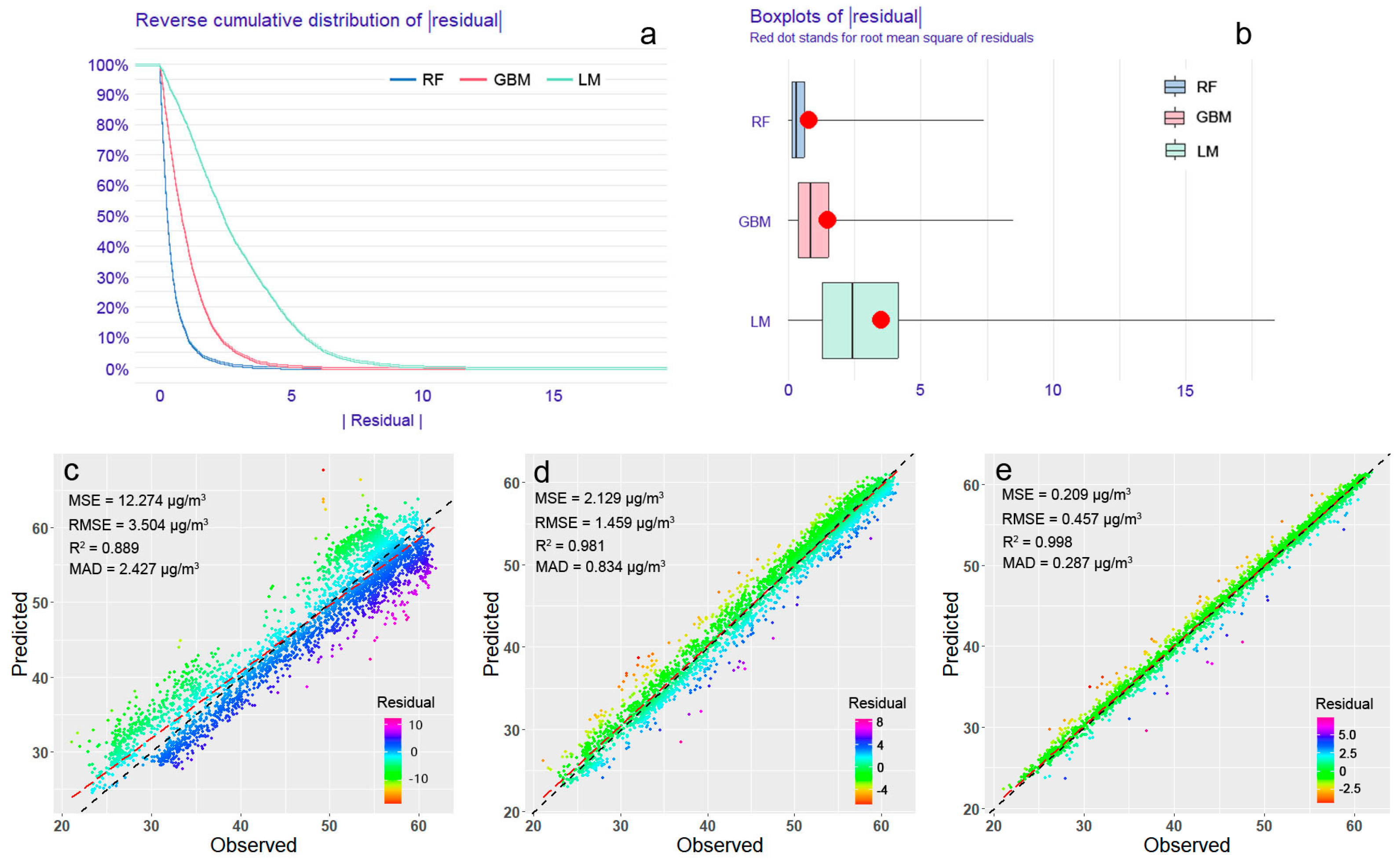
After testing the performance of the three global models using 30% Mdatas, we obtained several visualized results that show RF has outstanding performance. Reverse cumulative distribution of absolute residual shows that most of the samples in the RF have relatively small residuals, that is, only a few samples contributed large residuals, while a large number of samples in the LM had large residuals (Figure 3a). From the box-whisker plot, the mean (red dot) and range of values for the residuals of the ML algorithm were much smaller than those in the general regression model. RF also has better performance than GBM in ML. Moreover, the dispersion of scatter points from fitting observed and predicted values gradually decreased from LM to RF and RF has smaller MSE, RMSE, and MAD (Figure 3c–e).
The same training and testing scheme as Mdatas was carried out for Adatas. Both training and test samples had the same fitting results as Mdatas. Compared to LM and GBM, the RF model not only had better performance, but also had a narrower range of four model evaluation indexes, illustrating good stability (Figure 4). However, GBM’s test results were slightly better than its training results based on the comparison of training, test samples, and independent verification sample, while RF’s situation was the opposite (Figure 4, Table S3).

3.4. Evaluation of the Local Model

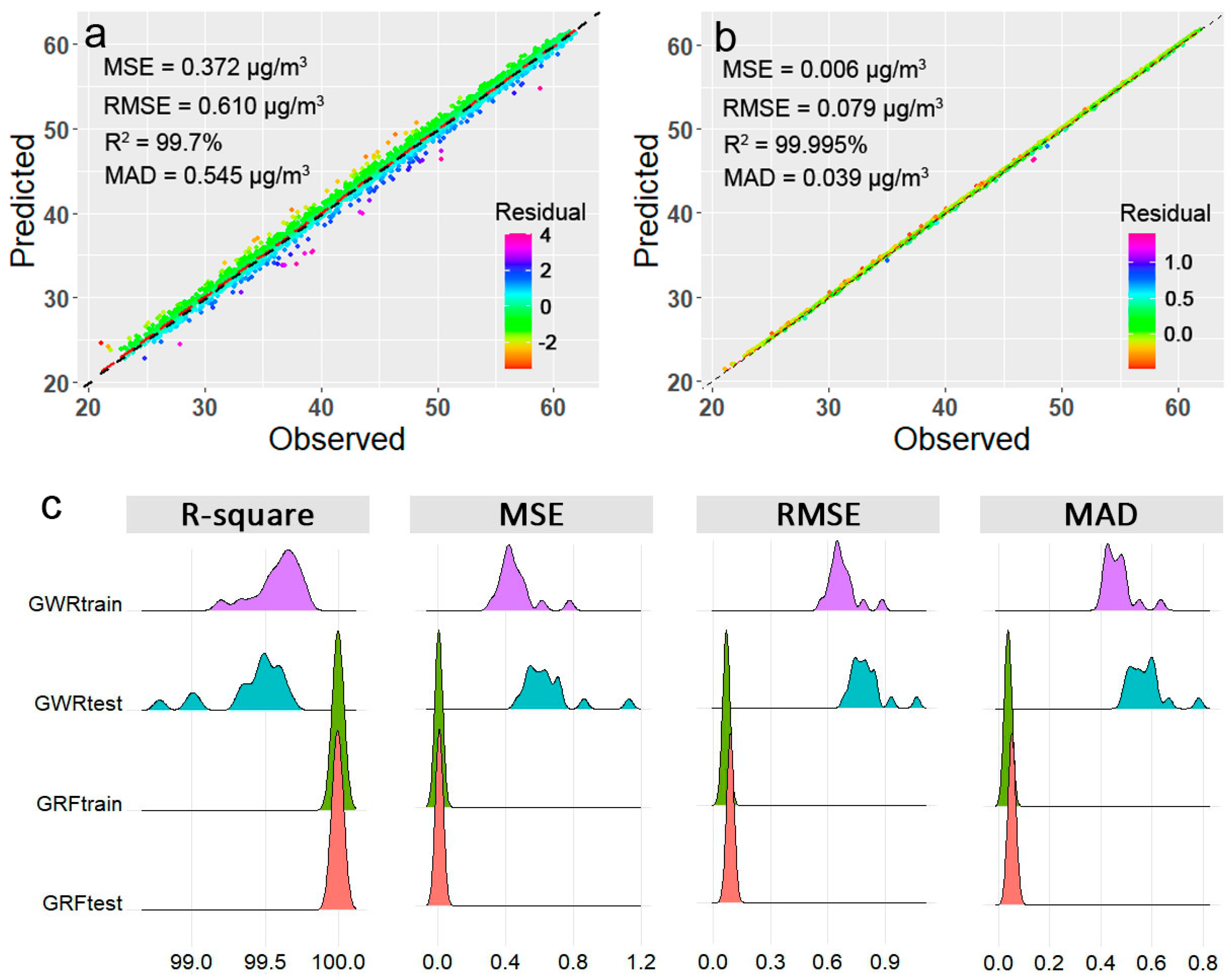
In total, 30% of the Mdata was used to test two local models and they had impressive performances: GWR: R2 = 99.7%; GWRF: R2 = 99.995% (Figure 5a,b). However, the advantages of GWRF were more significant, and its MSE, RMSE, and MAD were far less than those of GWR. The scatter plot also displays that the predicted PM2.5 concentration of GWRF was closer to the 1:1 line than that of GWR. In the model training and test of Adatas, it is notable that four parameters of GWR had a larger fluctuation range and more complex distribution than GWRF, which suggested that GWRF was more stable than GWR (Figure 5c). Furthermore, from the comparison of spatial autocorrelation of model residuals, we found that the GWRF’s residuals have smaller Global Moran’s I than the GWR’s residuals in the distance of 5 to 60 km for both training and test samples (Figure 6a,b). This result indicates that more spatial autocorrelation information was taken into consideration with GWRF. In the independent verification phase, GWRF performs far better than GWR (Table S3).

3.5. Comparison of Optimal Global and Local Models
Compared with the non-space version of RF, the model performance of GWRF has been greatly improved. Despite a modest increase in R2 (from 99.8% to 99.995%), MSE, RMSE, and MAD decline dramatically (MSE from 0.209 to 0.006; RMSE from 0.457 to 0.079; MAD from 0.287 to 0.039, respectively) (Figure 3c,e vs. Figure 5a,b). Figure 5 also indicates that the PM2.5 concentration predicted by GWRF was closer to the 1:1 line than RF. Furthermore, Figure 6a,b provides evidence that the Global Moran’s I of GWRF’s residuals were much smaller than RF’s residuals, suggesting that GWRF models take spatial autocorrelation into account more than RF models.
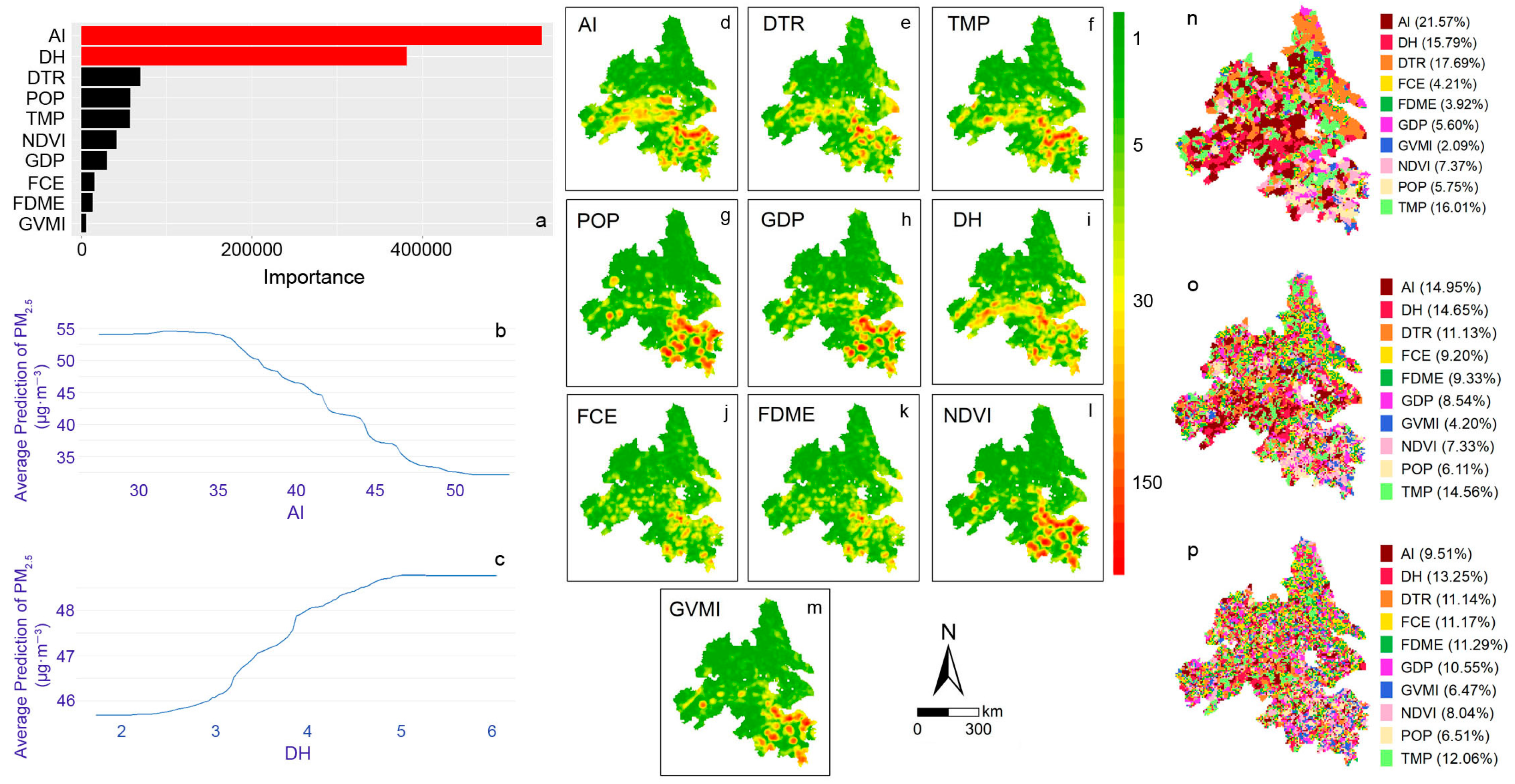
The results of complete Mdatas using RF suggest that AI and DH are the first and second significant important variables r based on the feature importance of IncNodePurity or Impurity (Figure 7a). Although the other variables did not display substantial influences, it can still be seen that climate factors and human activities have essential effects on PM2.5 concentration. A similar situation can also be seen in the order of importance calculated by Adatas (Figure S3). The importance ranking of AI and DH was relatively stable and maintained at a statistically significant level from 2003 to 2019, followed by DTR, POP, TMP, and GDP that were not significant in some years. In addition to the results of importance ranking for variables, we listed the local dependency graphs of two significantly important variables under the Mdatas sample (Figure 7b,c). AI was negatively affected in the PM2.5 exposure range of 32.5–55 μg/m3. On the contrary, DH was positively associated with PM2.5 in 45.75–48.75 μg/m3.
It is well known that the traditional global model cannot express the spatial heterogeneity response of the explanatory variable to the response variable. The geographically weighted method is an effective way to solve this problem. With the support of the GWRF, we calculated the complete sample of Mdatas and obtained the spatial distribution (Figure 7d–m) and descriptive statistics (Table 3) of all variables’ importance rankings. The high importance of all variables was observed in the YRD’s south and southeast. Among them, meteorological, human, and vegetation factors are pronounced, which means that the PM2.5 emissions in these areas are significantly associated with them. On the other hand, the primary impact of AI is in 21.75% of the regions, followed by DTR (17.69%), TMP (16.01%), and DH (15.79%) (Figure 7n–p). As the second important influencing variable of PM2.5, AI still accounted for 14.95% of the region, followed closely by DH and TMP (14.65% and 14.56%, respectively) (Figure 7o). For the regional proportion of the third important variable of PM2.5, the largest value is DH, followed by TMP, while FDME, FCE, and DTR had nearly the same lowest value (Figure 7p, Table 4). Meanwhile, the areas controlled by AI were principally situated in the YRD’s south, while the high PM2.5 concentration in the northern part was controlled primarily by DTR (Figure 7n) and TMP (Figure 7o). Although NDVI and GVMI had relatively few areas under strong control (Figure 7n–p), they hold an important influence in the southeast of the research district. Also, the analysis from the complete sample of Adatas shows that the area percentages of the first and second important influence areas of AI on PM2.5 concentration were 16.21%–22.72% and 12.93–17.4%, respectively, and DTR, TMP, and DH also had similar data distribution intervals. From 2003 to 2019, the most important influence area of AI and DTR on PM2.5 experienced a fluctuating upward trend, while the situation of TMP and DH was the opposite (Figure 8a). The second important influence area of these four explanatory factors all showed a wave-like rise (Figure 8b).
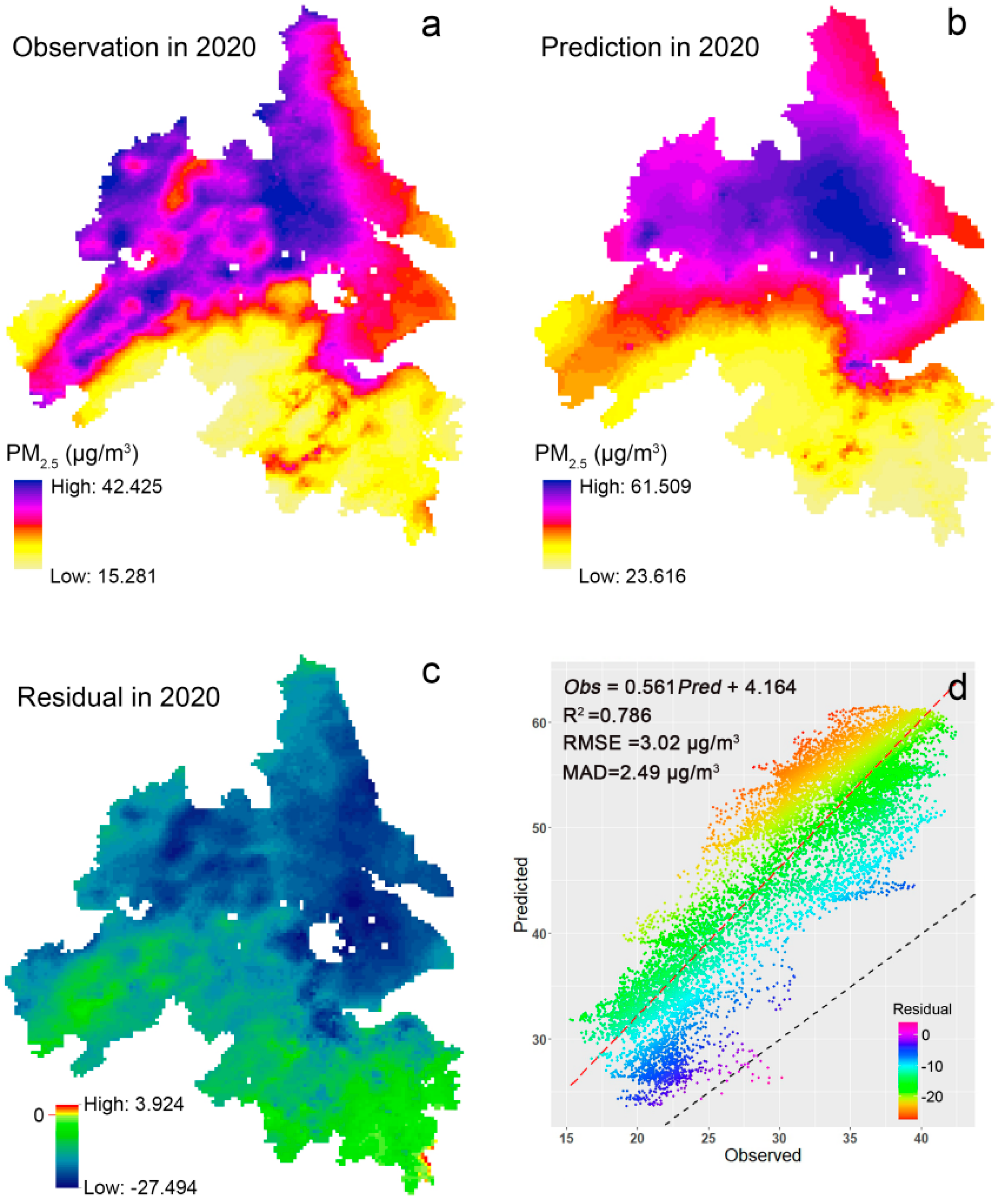
In the independent verification phase, GWRF performs well. The distribution of observed data was consistent with that predicted in 2020 (Figure 9a,b). Still, the range of values was different (For the observed value of 15.281–42.425 μg/m3, for the predicted value of 23.616–61.509 μg/m3). The fitted scatter plot (Figure 9c) describes a linear relationship between the observation and the results of the predicted value and R2 = 0.786. However, the estimated effect of the model from the residual distribution plot shows the model was underestimated (red to yellow area in Figure 9d) in only 0.146% of the area (scattered in the southeast corner). These are relatively few and challenging to observe.
Figure 7. The comparison of results for variables’ importance based on IncNodePurity of RF and GWRF with 17 years of mean data. (a) is permutation-based feature importance from RF; (b,c) are partial dependency plots of the significantly important variables of the RF model; (dm) are spatial variations of local feature importance of all variables in GWRF models. Higher values imply increased importance. (np) are the spatial distributions of the first, second, and third order of importance, respectively. Here, only the top three spatial distributions of importance are plotted. The rest of the rankings are detailed in Table 4.
Remotesensing 15 03826 g007
Figure 8. The proportion of areas for variables’ importance based on IncNodePurity of GWRF with annual data from 2003 to 2019. (a,b) are the local importance factors with the first and second, respectively.
Remotesensing 15 03826 g008
Figure 9. Comparison of observational data and GWRF predictions for 2020′s independent validation sample. (ac) are the spatial distribution of observation, prediction, and residual of PM2.5, respectively. (d) is the scatterplot of observed and predicted PM2.5 from GWRF.
Remotesensing 15 03826 g009

4. Discussion

4.1. Spatial Distribution and Clustering of PM2.5

We found high PM2.5 pollution and changes in 2015 from the study data, which is consistent with previous studies using site observation data from the YRD and also confirms the availability of our dataset [56]. According to Luo et al. [2], high concentrations of PM2.5 in 2015 are likely to be influenced by extreme weather (2015 was an El Niño year, and the peak intensity was in December 2015). PM2.5 has become the world’s fifth most prominent risk factor for death [27].
We conducted a hot spot analysis on the spatial clustering patterns of PM2.5 emissions and percentage change in the YRD in the period from 2003–2019. The results demonstrated a significant spatial clustering of PM2.5 in the YRD, with a large number of high-value areas distributed in the north and northwest (Figure 2a), and the distribution remained almost stable from 2003 to 2019 (Figure S4). This is consistent with what has been found in previous research based on site or MODIS raster data [2,12,17]. Yang et al. [7] confirmed the difference in PM2.5 exposure in the north and south of the YRD with the help of Nighttime Light Image (NTL). A popular explanation for the higher PM2.5 concentration in the north of the YRD is more urbanization and industrialization in this area [57]. The stable occurrence of cold spots in the southern region, on the one hand, is due to its hilly nature, with smaller human impact [10] and more forest cover, which helps improve air quality [58] (Figure 1). On the other hand, the meteorological conditions along the southeastern coast are conducive to clean air [56].
The highest percentage change of PM2.5 for 2019 compared to 2003 was found in the southeast, southwest, and west. These regions accounted for nearly 1/3 of the YRD (Figure 2b). The annual scale clustering distribution of percentage change, however, was not stable and the distribution of hot and cold spots was irregular (Figure S5), which is confirmed by Yan et al. [56]. Even though the guiding role of environmental policies (for instance the “Air Pollution Prevention and Control Action Plan” in 2013 and the “Ecological Environment Protection Plan for the Yangtze River Economic Belt” in 2017, [56]) formulated by national or local governments in recent years have reduced the range and variation of PM2.5 concentration in the YRD, some concerns about the findings are that there is still an annual growth rate of nearly 10–20% in some areas. There is also a high-value spatial state around the high-growth areas.
According to the comparison of Figure 2a,b, most of the northern half of the YRD is a PM2.5 concentration hotspot, but there are three spatial distribution states of PM2.5 changes in this area: (1) The area without significant clustering in the middle indicates that the change in PM2.5 in this area is spatially discrete; from Figure 1c, it can also be seen that there are three situations of increase, unchanged, and improvement in PM2.5 in this area at the same time. (2) The cold spot area on the right is the area where PM2.5 changes are low-value accumulation. The high industrialization and urbanization of the northern half is one reason for the high PM2.5 in this region [57], while the monsoon in the coastal region creates opportunities for the improvement of PM2.5 in the east [56]. (3) A small number of hot spots of PM2.5 on the left are also gathering areas where PM2.5 increases. On the one hand, this place is the manufacturing center of China (Hefei) [7], with a large number of factories and high motor vehicle traffic [12]. On the other hand, the pollutants transmitted from the eastern coast make for the high concentration of PM2.5 in this area, which is not easy to reduce [12,56]. Although the PM2.5 change hot spots in the PM2.5 cold spot area in the south of the YRD show high-value clustering, these changes are concentrated in the range of 10–20%. We have reason to believe that this discovery can help the government to formulate air pollution prevention measures suitable for different regions.

4.2. Comparison of PM2.5 Prediction Models

This study considered five modeling methods to train the relationship between PM2.5 concentration and predictors under the same predictor variables and samples. The global model results tell us that compared with the classical regression model, the obvious advantages of ML were highlighted by the smaller residual range (Figure 3c–e) [59]. Among the ML algorithms we used, RF showed more excellent results than GBM in both Mdatas and Adatas. Similar results were obtained by Danesh Yazdi et al. [1], who used different ML methods to analyze the control effect of environmental factors on PM2.5 in London. They believe that RF is better than GBM at simulating the explanation of PM2.5 changes by environmental factors. They believe that GBM was not suitable for predicting long-term PM2.5 concentration. Note that the test results of GBM are slightly better than the training results, while the RF model is the opposite, which shows that GBM has a slight advantage in the generalization ability of the model. However, it is undeniable that each decision tree in RF can be trained independently, so it can be directly processed in parallel to save calculation time. In contrast, the training of each tree in GBM relies on the operations of the previous tree without the help of other parallel techniques [49,60].
The local version of LM has a more significant improvement than the global LM, but the geographically weighted regression’s sensitivity to multicollinearity has not been solved [25]. GWRF has advantages and robustness over GWR in both Mdatas and Adatas (Figure 5). Meanwhile, the spatial autocorrelation analysis of residuals suggests that the residuals of GWRF are more random than those of GWR and global RF models. This result confirms that GWRF effectively captures the spatial heterogeneity [26], which can better model and predict PM2.5 in the YRD. Furthermore, the validation of the model by the independent validation dataset also yielded promising results, a validation phase we did not see in most studies [5,16,61]. Unlike most of the model underestimates in previous studies [5,61], we can see that the model has an overestimation of 99.854% for the data in 2020. One possible explanation is that the process of human interference has been associated with the COVID-19 pandemic policy of regional closure. We will also test this possibility in our next research. We also noted the spatiotemporal random forest model developed by Wei et al. [61] and applied it to PM2.5 prediction studies in China. It is undeniable that the model has achieved excellent results through the input of space and time, but it only simply considers the space-time information [5] and does not effectively integrate the local effects of spatial objects. Moreover, our annual scale research is not applicable to the spatiotemporal RF algorithm (daily scale). In the future, we will consider comparing and analyzing the modeling results of two kinds of spatial RF based on daily scale data.

4.3. The Influencing Factors of PM2.5

Global RF only provides global importance ranking and significant important variables. However, we are told by Yan et al. [56] that this is unfair because not all variable influences are globally important according to the results of GWRF. For example, drought and human disturbance only have important effects in the parts of central and southern regions. Similarly, the forest cover and low average PM2.5 emissions in the southern and southeastern areas suggest that only some variables are useful (Figure 1a,b). The influence distribution map of NDVI and GVMI tells us that these regions are almost under their control (Figure 7). Compared with the low vegetation (shrub and arable land) in the northern region, the southern forest has a larger canopy surface area, and the effect of arbor vegetation on the interception and absorption of particulate matter in the atmosphere is better than that of other underlying surfaces on land [31].
In this study, climate factors are important predictors of PM2.5 concentration, which confirms that the high standard management of air pollution is inseparable from climate collaborative management. The effects of drought, temperature difference, and average temperature on PM2.5 are of high importance, especially drought, which confirms the report of Wang et al. [62]. In the southern and southeastern regions where forest vegetation is distributed, it is also an important area affected by drought (Figure 1a and Figure 7d). With the emergence of extreme droughts worldwide, areas affected by drought are also slowly increasing (Figure 8). Vegetation in drought shrinks its stomata to ensure its water demand, resulting in reduced absorption and capture of PM2.5 in the air [20,34], and the reduction in total leaf area on longer time scales also poses a challenge to larger areas of sedimentation for PM2.5. Moreover, the disturbance of air turbulence and the maintenance of humidity in the southern woodlands ensure that they absorb atmospheric particles more effectively than low-growing vegetation. Also, we noticed the results of Demetillo et al. [34] in an experimental study showing that drought also was essential to reduce the volatilization of volatile organic compounds, precursors of O3 and PM2.5, from plants. Unfortunately, GWRF does not provide results on the partial dependency relationship of variables, and we currently cannot know how AI affects PM2.5 emissions in the GWRF model, which will become our next research task. In addition, our research also found that more biomass burning caused by drought did not have much impact on the PM2.5 concentration of the YRD. Another climate driving PM2.5 with an upward trend is the diurnal temperature range. It has also been observed that air visibility is related to a change in the difference between the maximum and minimum temperature [63]. One of the reasons is that the large diurnal temperature range promotes the emergence of an inversion layer which hinders the vertical flow of air and makes it difficult for pollutants to diffuse in the surface atmosphere [20,63]. Another reason is that the smaller DTR stimulates the urban heat island and makes the air quality worse, especially in cities with high energy consumption and exhaust emissions. [31]. Different from the findings of Jin et al. [3], our research did not find the prominent and important influence of traditional social indicators, namely POP and GDP, on PM2.5 in our research. However, as a representative of human impact on ecology, the human ecological disturbance index (DH) is prominent among the critical influencing factors of PM2.5 (Figure 7, Table 3 and Table 4).
A simple increase or decrease in population and GDP may not directly reflect their influence on PM2.5 pollution. The human disturbance index calculated by land use type effectively explains the spatial distribution of PM2.5 in our research (Figure 7). A similar result was obtained by Geng et al. [64]. Unlike classical land-use regression (LUR) models, we assigned weights to different types of parcels within the sample cells to measure human disturbance as predictors [45]. The LUR model is a multiple linear regression based on the proportion of land use type as a predictive variable. On the one hand, LUR assumes a linear relationship between PM2.5 and land use type, while this relationship is not always linear. Meanwhile, the model ignores the collinearity between the variables of various land use types [14], which interferes with the predictor’s interpretation of response variables and thus affects the results of the modeling. In a follow-up study, we will plan the comparison of the modeling of these two cases. In addition, we also observe a year-over-year decrease in areas where human disturbance significantly affects PM2.5, which is mainly due to the increased efforts of the government to improve the environment and ecological quality [56].

4.4. Limitations

Nevertheless, there are still some limitations to our study. First, GWRF is an improved space-based ML method, but currently GWRF still needs to be improved in practical applications: (1) Calculate the significance level of variable importance like the global RF method; (2) Lack of partial dependence to understand how explanatory variables affect PM2.5 concentration; (3) There are no methods or criteria for judging spatial non-stationarity. Second, limited by the acquisition of previous data, this study lacks the relationship between air pollution and a wide range of human activities and other environmental issues (such as urban heat islands), which will be included in future research. Furthermore, information related to environmental protection policy was not considered in this study. We all know that since 2013, a large number of protective measures and procedures have restricted air pollutants, including PM2.5. Fourthly, it is known that drought affects pollutants in the atmosphere through vegetation, but the specific impact mechanism still needs to be reported, which will also be the focus of subsequent efforts. Finally, the sampling unit of this study is 5 km × 5 km, and the evaluation of the impact of smaller or larger size grids on modeling and analysis results will also be included in our future research plan.

5. Conclusions

We obtained satellite raster data and considered hot spot analysis to display the spatial distribution and percentage change of PM2.5 in the YRD from 2003 to 2019. Five methods were then used to model, test, and verify the data of the YRD for 18 years. The following conclusions were obtained after analysis: (1) The high PM2.5 concentration cluster in the western and northwestern areas of the YRD had little change during 2003–2019. Compared with 2003, PM2.5 increased by 10 to 20 percent in the southeast, southwest, and western regions in 2019. The hot spot for percentage change of PM2.5 in 2019 was principally located in the southwest and southeast of the YRD, while the interannual change showed a changeable spatial distribution pattern. (2) GWRF had the most outstanding performance in the training and testing stages of modeling PM2.5 exposure among all the models, and compared with global RF, it realized the spatialization of variable importance ranking. (3) Based on the results of explanatory variable analysis, climate factors and human activities were identified to be the most critical drivers of PM2.5 concentration. Among them, drought, temperature, temperature difference, and the degree of human interference were the critical and most extensive influencing factors of PM2.5 in the YRD. Compared with other factors, the essential influence areas of drought, temperature, and temperature difference on the YRD’s PM2.5 experienced fluctuating growth. This result suggests that drought and air temperature differences need to be taken into account in the PM2.5 prediction under warming and drying worldwide to help regulators and policymakers formulate prevention and control measures. With the recovery and increase in the frequency of interference from human activities on ecosystems after the COVID-19 pandemic, the solid explanatory power of comprehensive ecological indicators on the distribution of PM2.5 will be a crucial indicator worth considering by decision-making departments.

Supplementary Materials

The following supporting information can be downloaded at: https://www.mdpi.com/article/10.3390/rs15153826/s1, Figure S1 The graph of model error with the number of trees (ntree) and mtry. Figure S2 Spatial distribution of each variable. Figure S3 The annual effect of variables on PM2.5 concentration using RF model. Figure S4 The annual geographical clusters from Getis-Ord Gi* of PM2.5 concentration. Figure S5 The annual geographical clusters from Getis-Ord Gi* of percent change of PM2.5. Table S1 The proportion of annual geographic cluster significance level regions for PM2.5 concentrations from Getis-Ord Gi*. Table S2 The proportion of annual geographic cluster significance level regions for percent change of PM2.5 from Getis-Ord Gi*. Table S3 The validation results for 5 models using independent validation dataset (2020′s data).

Author Contributions

Conceptualization, Z.S. and Y.C.; methodology, Z.S. and Z.X.; validation, Y.C. and L.L.; investigation, S.L. and S.W.; data curation, Z.S. and L.Y.; formal analysis, Z.S. and Z.L.; writing—original draft preparation, Z.S.; writing—review and editing, Y.C., H.H. and L.L.; supervision, S.L. and Y.C.; funding acquisition, Z.S., Z.X. and S.W. All authors have read and agreed to the published version of the manuscript.

Funding

This research was funded by the Young and Middle-aged Teacher Education Research Project of Fujian Province (JAT220690); Special Research Project on Innovative Application of Virtual Simulation Technology in Vocational Education Teaching (ZJXF2022056); Natural Science Foundation of Guangdong Province, China (2021A1515010946); Forestry Science and Technology Innovation of Guangdong Province, China (2020KJCX003).

Data Availability Statement

The data and statistical analysis methods are available upon request from the corresponding author.

Acknowledgments

We would like to thank the editor and anonymous reviewers for their useful advice that helped to improve the manuscript.

Conflicts of Interest

The authors declare no conflict of interest. The funders had no role in the design of the study; in the collection, analyses, or interpretation of the data; in the writing of the manuscript; or in the decision to publish the results.

References

  1. Danesh Yazdi, M.; Kuang, Z.; Dimakopoulou, K.; Barratt, B.; Suel, E.; Amini, H.; Lyapustin, A.; Katsouyanni, K.; Schwartz, J. Predicting fine particulate matter (PM2.5) in the greater London area: An ensemble approach using machine learning methods. Remote Sens. 2020, 12, 914. [Google Scholar] [CrossRef] [Green Version]
  2. Luo, Y.; Teng, M.; Yang, K.; Zhu, Y.; Zhou, X.; Zhang, M.; Shi, Y. Research on PM2.5 estimation and prediction method and changing characteristics analysis under long temporal and large spatial scale—A case study in China typical regions. Sci. Total Environ. 2019, 696, 133983. [Google Scholar]
  3. Jin, H.; Zhong, R.; Liu, M.; Ye, C.; Chen, X. Spatiotemporal distribution characteristics of PM2.5 concentration in China from 2000 to 2018 and its impact on population. J. Environ. Manag. 2022, 323, 116273. [Google Scholar] [CrossRef] [PubMed]
  4. Bera, B.; Bhattacharjee, S.; Sengupta, N.; Saha, S. PM2.5 concentration prediction during COVID-19 lockdown over Kolkata metropolitan city, India using MLR and ANN models. Environ. Chall. 2021, 4, 100155. [Google Scholar] [CrossRef]
  5. He, W.; Meng, H.; Han, J.; Zhou, G.; Zheng, H.; Zhang, S. Spatiotemporal PM2.5 estimations in China from 2015 to 2020 using an improved gradient boosting decision tree. Chemosphere 2022, 296, 134003. [Google Scholar] [CrossRef]
  6. Yan, X.; Zang, Z.; Jiang, Y.; Shi, W.; Guo, Y.; Li, D.; Zhao, C.; Husi, L. A spatial-temporal interpretable deep learning model for improving interpretability and predictive accuracy of satellite-based PM2.5. Environ. Pollut. 2021, 273, 116459. [Google Scholar] [CrossRef]
  7. Yang, Z.; Zdanski, C.; Farkas, D.; Bang, J.; Williams, H. Evaluation of aerosol optical depth (AOD) and PM2.5 associations for air quality assessment. Remote Sens. Appl. 2020, 20, 100396. [Google Scholar] [CrossRef]
  8. Wei, J.; Huang, W.; Li, Z.; Xue, W.; Peng, Y.; Sun, L.; Cribb, M. Estimating 1-km-resolution PM2.5 concentrations across China using the space-time random forest approach. Remote Sens. Environ. 2019, 231, 111221. [Google Scholar] [CrossRef]
  9. Hu, X.; Belle, J.H.; Meng, X.; Wildani, A.; Waller, L.A.; Strickland, M.J.; Liu, Y. Estimating PM2.5 concentrations in the conterminous United States using the random forest approach. Environ. Sci. Technol. 2017, 51, 6936. [Google Scholar] [CrossRef]
  10. Liu, J.; Weng, F.; Li, Z. Satellite-based PM2.5 estimation directly from reflectance at the top of the atmosphere using a machine learning algorithm. Atmos. Environ. 2019, 208, 113–122. [Google Scholar] [CrossRef]
  11. van Donkelaar, A.; Martin, R.V.; Li, C.; Burnett, R.T. Regional estimates of chemical composition of fine particulate matter using a combined geosciencestatistical method with information from satellites, models, and monitors. Environ. Sci. Technol. 2019, 53, 2595–2611. [Google Scholar] [CrossRef] [Green Version]
  12. Su, Z.; Lin, L.; Chen, Y.; Hu, H. Understanding the distribution and drivers of PM2.5 concentrations in the Yangtze River Delta from 2015 to 2020 using Random Forest Regression. Environ. Monit. Assess. 2022, 94, 284. [Google Scholar] [CrossRef]
  13. Wang, X.; Sun, W. Meteorological parameters and gaseous pollutant concentrations as predictors of daily continuous PM2.5 concentrations using deep neural network in Beijing–Tianjin–Hebei, China. Atmos. Environ. 2019, 211, 128–137. [Google Scholar] [CrossRef]
  14. Kerckhoffs, J.; Hoek, G.; Portengen, L.; Brunekreef, B.; Vermeulen, R.C.H. Performance of prediction algorithms for modeling outdoor air pollution spatial surfaces. Environ. Sci. Technol. 2019, 53, 1413–1421. [Google Scholar] [CrossRef] [PubMed] [Green Version]
  15. Zhang, T.; He, W.; Zheng, H.; Cui, Y.; Song, H.; Fu, S. Satellite-based ground PM2.5 estimation using a gradient boosting decision tree. Chemosphere 2021, 268, 128801. [Google Scholar] [CrossRef]
  16. Zhang, P.; Ma, W.; Wen, F.; Liu, L.; Yang, L.; Song, J.; Wang, N.; Liu, Q. Estimating PM2.5 concentration using the machine learning GA-SVM method to improve the land use regression model in Shaanxi, China. Ecotox. Environ. Safe. 2021, 225, 112772. [Google Scholar] [CrossRef] [PubMed]
  17. Dai, H.; Huang, G.; Wang, J.; Zeng, H.; Zhou, F. Spatio-temporal characteristics of PM2.5 concentrations in china based on multiple sources of data and LUR-GBM during 2016–2021. Int. J. Environ. Res. Public Health 2022, 19, 6292. [Google Scholar] [CrossRef]
  18. Luo, Z.; Huang, F.; Liu, H. PM2.5 concentration estimation using convolutional neural network and gradient boosting machine. J. Environ. Sci. 2020, 98, 85–93. [Google Scholar] [CrossRef]
  19. Huang, G.; Li, X.; Zhang, B.; Ren, J. PM2.5 concentration forecasting at surface monitoring sites using GRU neural network based on empirical mode decomposition. Sci. Total Environ. 2021, 768, 144516. [Google Scholar] [CrossRef]
  20. Su, Z.; Xu, Z.; Lin, L.; Chen, Y.; Hu, H.; Wei, S.; Luo, S. Exploration of the Contribution of Fire Carbon Emissions to PM2.5 and Their Influencing Factors in Laotian Tropical Rainforests. Remote Sens. 2022, 14, 4052. [Google Scholar] [CrossRef]
  21. He, Q.; Huang, B. Satellite-based mapping of daily high-resolution ground PM2.5 in China via space-time regression modeling. Remote Sens. Environ. 2018, 206, 72–83. [Google Scholar] [CrossRef]
  22. Quiñones, S.; Goyal, A.; Ahmed, Z.U. Geographically weighted machine learning model for untangling spatial heterogeneity of type 2 diabetes mellitus (T2D) prevalence in the USA. Sci. Rep. 2021, 11, 6955. [Google Scholar] [CrossRef] [PubMed]
  23. Hengl, T.; Nussbaum, M.; Wright, M.N.; Heuvelink, G.B.M.; Gräler, B. Random Forest as a Generic Framework for Predictive Modeling of Spatial and Spatio-Temporal Variables. PeerJ 2018, 6, e5518. [Google Scholar] [CrossRef] [PubMed] [Green Version]
  24. Georganos, S.; Grippa, T.; Gadiaga, A.N.; Linard, C.; Lennert, M.; Vanhuysse, S.; Odhiambo Mboga, N.; Wolff, E.; Kalogirou, S. Geographical random forests: A spatial extension of the random forest algorithm to address spatial heterogeneity in remote sensing and population modelling. Geocarto Int. 2019, 36, 121–136. [Google Scholar] [CrossRef] [Green Version]
  25. Santos, F.; Graw, V.; Bonilla, S. A geographically weighted random forest approach for evaluate forest change drivers in the Northern Ecuadorian Amazon. PLoS ONE 2019, 14, e0226224. [Google Scholar] [CrossRef]
  26. Khan, S.N.; Li, D.; Maimaitijiang, M. A geographically weighted random forest approach to predict corn yield in the US corn belt. Remote Sens. 2022, 14, 2843. [Google Scholar] [CrossRef]
  27. Meng, X.; Hand, J.L.; Schichtel, B.A.; Liu, Y. Space-time trends of PM2.5 constituents in the conterminous United States estimated by a machine learning approach, 2005–2015. Environ. Int. 2018, 121, 1137–1147. [Google Scholar] [CrossRef]
  28. Kaur, M.; Nagpal, A.K. Evaluation of air pollution tolerance index and anticipated performance index of plants and their application in development of green space along the urban areas. Environ. Sci. Pollut. Res. 2017, 24, 18881–18895. [Google Scholar] [CrossRef]
  29. Hua, Y.; Cheng, Z.; Wang, S.; Jiang, J.; Chen, D.; Cai, S.; Fu, X.; Chen, C.; Xu, B.; Yu, J. Characteristics and source apportionment of PM2.5 during a fall heavy haze episode in the Yangtze River Delta of China. Atmos. Environ. 2015, 123, 380–391. [Google Scholar] [CrossRef]
  30. Zhang, Q.; Zheng, Y.; Tong, D.; Shao, M.; Hao, J. Drivers of improved PM2.5 air quality in China from 2013 to 2017. Proc. Natl. Acad. Sci. USA 2019, 116, 201907956. [Google Scholar] [CrossRef] [Green Version]
  31. Balogun, A.; Tella, A.; Baloo, L.; Adebisi, N. A review of the inter-correlation of climate change, air pollution and urban sustainability using novel machine learning algorithms and spatial information science. Urban Clim. 2021, 40, 100989. [Google Scholar] [CrossRef]
  32. Xue, T.; Zheng, Y.; Geng, G.; Zheng, B.; Jiang, X.; Zhang, Q.; He, K. Fusing observational, satellite remote sensing and air quality model simulated data to estimate spatiotemporal variations of PM2.5 exposure in China. Remote Sens. 2017, 9, 221. [Google Scholar] [CrossRef] [Green Version]
  33. Hammer, M.S.; van Donkelaar, A.; Li, C.; Lyapustin, A.; Sayer, A.M.; Hsu, N.C.; Levy, R.C.; Garay, M.J.; Kalashnikova, O.V.; Kahn, R.A.; et al. Global estimates and long-term trends of fine particulate matter concentrations (1998–2018). Environ. Sci. Technol. 2020, 54, 7879–7890. [Google Scholar] [CrossRef]
  34. Demetillo, M.A.G.; Anderson, J.F.; Geddes, J.A.; Yang, X.; Najacht, E.Y.; Herrera, S.A.; Kabasares, K.M.; Kotsakis, A.E.; Lerdau, M.T.; Pusede, S.E. Observing severe drought influences on ozone air pollution in California. Environ. Sci. Technol. 2019, 53, 4695–4706. [Google Scholar] [CrossRef] [PubMed]
  35. Berg, A.; McColl, K.A. No projected global drylands expansion under greenhouse warming. Nat. Clim. Chang. 2021, 11, 331–337. [Google Scholar] [CrossRef]
  36. Harris, I.; Osborn, T.J.; Jones, P.; Lister, D. Version 4 of the CRU TS monthly high-resolution gridded multivariate climate dataset. Sci. Data 2020, 7, 109. [Google Scholar] [CrossRef] [Green Version]
  37. Martinez, A.I.; Labib, S.M. Demystifying normalized difference vegetation index (NDVI) for greenness exposure assessments and policy interventions in urban greening. Environ. Res. 2023, 220, 115155. [Google Scholar] [CrossRef]
  38. Zubieta, R.; Ccanchi, Y.; Alejandra Martínez, A.; Saavedra, M.; Norabuena, E.; Alvarez, S.; Ilbay, M. The role of drought conditions on the recent increase in wildfire occurrence in the high Andean regions of Peru. Int. J. Wildland Fire 2023, 32, 531–544. [Google Scholar] [CrossRef]
  39. Du, X. Research on Vegetation Leaf Water Monitoring by Remote Sensing and Spatio-Temporai Character Analysis; Institute of Remote Sensing and Digital Earth Chinese Academy of Sciences: Beijing, China, 2006. (In Chinese) [Google Scholar]
  40. Su, Z.; Zheng, L.; Luo, S.; Tigabu, M.; Guo, F. Modeling wildfire drivers in Chinese tropical forest ecosystems using global logistic regression and geographically weighted logistic regression. Nat. Hazards 2021, 108, 1317–1345. [Google Scholar] [CrossRef]
  41. Zhang, X.; Brandt, M.; Tong, X.; Ciais, P.; Yue, Y.; Xiao, X.; Zhang, W.; Wang, K.; Fensholt, R. A large but transient carbon sink from urbanization and rural depopulation in China. Nat. Sustain. 2022, 5, 321–328. [Google Scholar] [CrossRef]
  42. Nethery, R.C.; Rushovich, T.; Peterson, E.; Chen, J.T.; Waterman, P.D.; Krieger, N.; Waller, L.; Coull, B.A. Comparing denominator sources for real-time disease incidence modeling: American Community Survey and WorldPop. SSM Popul. Health 2021, 14, 100786. [Google Scholar] [CrossRef] [PubMed]
  43. Guo, F.; Innes, L.J.; Wang, G.; Ma, X.; Sun, L.; Hu, H.; Su, Z. Historic distribution and driving factors of human-caused fires in the Chinese boreal forest between 1972 and 2005. J. Plant. Ecol. 2015, 8, 480–490. [Google Scholar] [CrossRef] [Green Version]
  44. Liu, S.; Liu, L.; Wu, X.; Hou, X.; Zhao, S.; Liu, G. Quantitative evaluation of human activity intensity on the regional ecological impact studies. Acta Ecol. Sin. 2018, 38, 6797–6809. (In Chinese) [Google Scholar]
  45. Beyhan, E.; Yarci, C.; Yilmaz, A. Investigation of hemeroby degree of vegetation in urban transport areas: The case of izmit (Kocaeli). Front. Life Sci. Relat. Technol. 2020, 1, 28–34. [Google Scholar]
  46. Prosperi, P.; Bloise, M.; Tubiello, F.N.; Conchedda, G.; Rossi, S.; Boschetti, L.; Salvatore, M.; Bernoux, M. New estimates of greenhouse gas emissions from biomass burning and peat fires using MODIS Collection 6 burned areas. Clim. Chang. 2020, 161, 415–432. [Google Scholar] [CrossRef] [Green Version]
  47. ESRI. ArcGIS Desktop, Release 10.6.1.; Environmental Systems Research Institute: Redlands, CA, USA, 2019. [Google Scholar]
  48. Ge, L.; Li, Y.; Wu, Y.; Fan, Z.; Song, Z. Differential Diagnosis of Rosacea Using Machine Learning and Dermoscopy. Clin. Cosmet. Inv. Derm. 2022, 15, 1465–1473. [Google Scholar] [CrossRef]
  49. Breiman, L. Random Forests. Mach. Learn. 2001, 45, 5–32. [Google Scholar] [CrossRef] [Green Version]
  50. Cutler, D.R.; Edwards, T.C.; Beard, K.H.; Cutler, A.; Hess, K.T.; Gibson, J. Random forests for classifcation in ecology. Ecology 2007, 88, 2783–2792. [Google Scholar] [CrossRef]
  51. Chen, Y.; Zheng, W.; Li, W.; Huang, Y. Large group activity security risk assessment and risk early warning based on random forest algorithm. Pattern. Recogn. Lett. 2021, 144, 1–5. [Google Scholar] [CrossRef]
  52. Zhan, Y.; Luo, Y.; Deng, X.; Zhang, K.; Zhang, M.; Grieneisen, M.L.; Di, B. Satellite-based estimates of daily NO2 exposure in China using hybrid random forest and spatiotemporal Kriging model. Environ. Sci. Technol. 2018, 52, 4180. [Google Scholar] [CrossRef]
  53. Zhang, B.; Tian, J.; Pei, S.; Chen, Y.; He, X.; Dong, Y.; Zhang, L.; Mo, X.; Huang, W.; Cong, S.; et al. Machine Learning-Assisted System for Thyroid Nodule Diagnosis. Thyroid 2019, 29, 858–867. [Google Scholar] [CrossRef] [PubMed]
  54. Wang, H.; Seaborn, T.; Wang, Z.; Caudil, C.C.; Link, T.E. Modeling tree canopy height using machine learning over mixed vegetation landscapes. Int. J. Appl. Earth Obs. 2021, 101, 102353. [Google Scholar] [CrossRef]
  55. Rodrigues, M.; de la Riva, J.; Fotheringham, S. Modeling the spatial variation of the explanatory factors of human-caused wildfires in Spain using geographically weighted logistic regression. Appl. Geogr. 2014, 48, 52–63. [Google Scholar] [CrossRef]
  56. Yan, J.; Tao, F.; Zhang, S.; Lin, S.; Zhou, T. Spatiotemporal distribution characteristics and driving forces of PM2.5 in three urban agglomerations of the Yangtze River Economic Belt. Int. J. Environ. Res. Public Health 2021, 18, 2222. [Google Scholar] [CrossRef] [PubMed]
  57. Chen, J.; Li, C.; Ristovski, Z.; Milic, A.; Gu, Y.; Islam, M.S.; Wang, S.; Hao, J.; Zhang, H.; He, C.; et al. A review of biomass burning: Emissions and impacts on air quality, health and climate in China. Sci. Total Environ. 2017, 579, 1000–1034. [Google Scholar] [CrossRef] [PubMed] [Green Version]
  58. She, Q.; Peng, X.; Xu, Q.; Long, L.; Wei, N.; Liu, M.; Jia, W.; Zhou, T.; Han, J.; Xiang, W. Air quality and its response to satellite-derived urban form in the Yangtze River Delta, China. Ecol. Indic. 2017, 75, 297–306. [Google Scholar] [CrossRef]
  59. Biancofiore, F.; Busilacchio, M.; Verdecchia, M.; Tomassetti, B.; Aruffo, E.; Bianco, S.; Di Tommaso, S.; Colangeli, C.; Rosatelli, G.; Di Carlo, P. Recursive neural network model for analysis and forecast of PM10 and PM2.5. Atmos. Pollut. Res. 2017, 8, 652–659. [Google Scholar] [CrossRef]
  60. Friedman, J.H. Greedy function approximation: A gradient boosting machine. Ann. Stat. 2001, 29, 1189–1232. [Google Scholar] [CrossRef]
  61. Wei, J.; Li, Z.; Pinker, R.T.; Wang, J.; Sun, L.; Xue, W.; Li, R.; Cribb, M. Himawari-8-derived diurnal variations in ground-level PM2.5 pollution across China using the fast space-time Light Gradient Boosting Machine (LightGBM). Atmos. Chem. Phys. 2021, 21, 7863–7880. [Google Scholar] [CrossRef]
  62. Wang, Y.; Xie, Y.; Dong, W.; Ming, Y.; Wang, J.; Shen, L. Adverse effects of increasing drought on air quality via natural processes. Atmos. Chem. Phys. 2017, 17, 12827–12843. [Google Scholar] [CrossRef] [Green Version]
  63. Feng, X.; Wei, S.; Wang, S. Temperature inversions in the atmospheric boundary layer and lower troposphere over the Sichuan Basin, China: Climatology and impacts on air pollution. Sci. Total Environ. 2020, 726, 138579. [Google Scholar] [CrossRef] [PubMed]
  64. Geng, G.; Zhang, Q.; Martin, R.V.; van Donkelaar, A.; Huo, H.; Che, H.; Lin, J.; He, K. Estimating long-term PM2.5 concentrations in China using satellite-based aerosol optical depth and a chemical transport model. Remote Sens. Environ. 2015, 166, 262–270. [Google Scholar] [CrossRef]
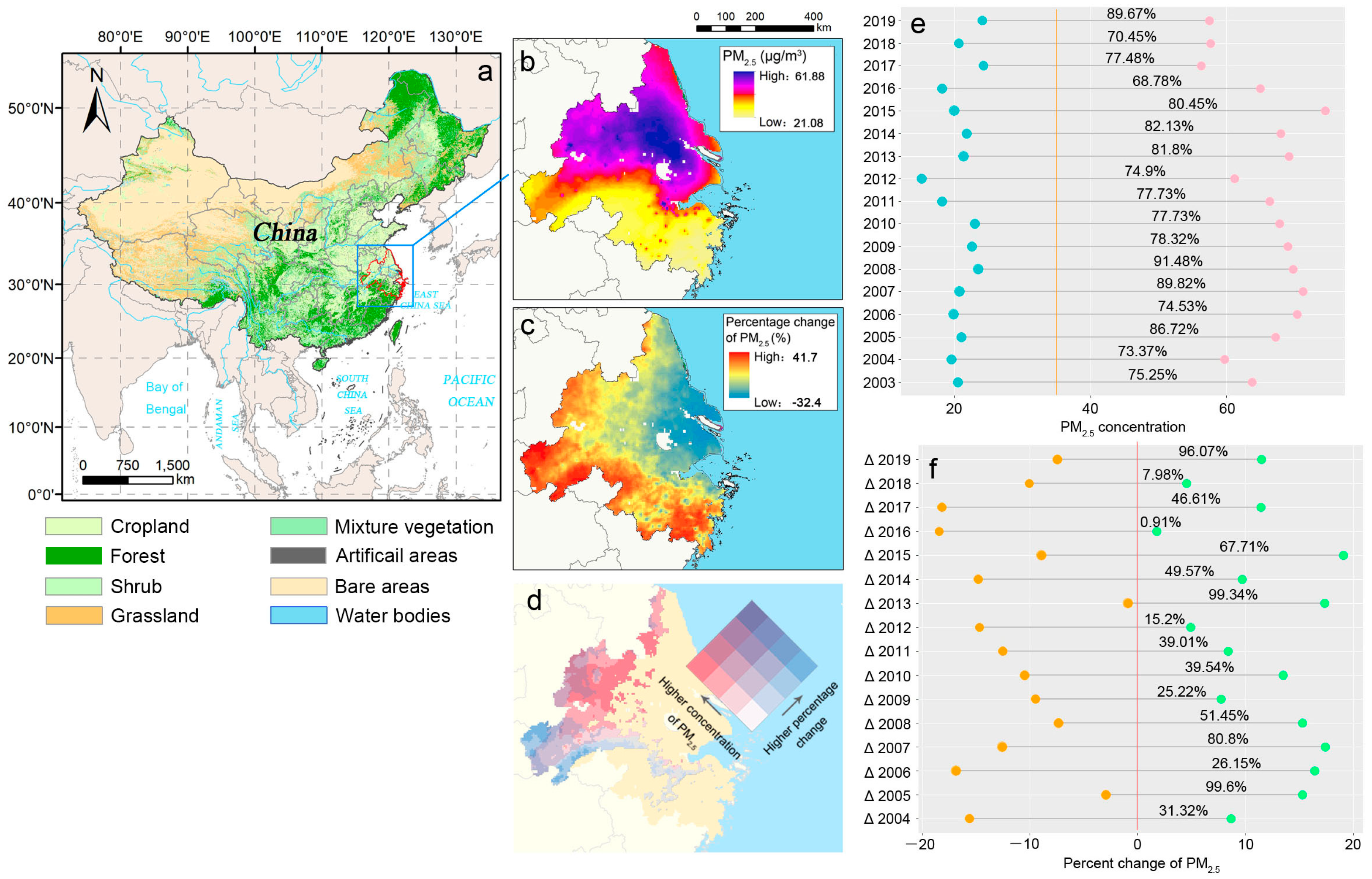
Figure 1. Study Area. (a) is the distribution of vegetation types in China and the red border represents the study area. (b) is the spatial distribution of average concentration for PM2.5 in the study area from 2003 to 2019. (c) is the average percent change from the years 2003 to 2019. (d) shows the overlapping distribution of the area where the average concentration of PM2.5 exceeds 35 μg/m3 in 17 years and the area where the percentage of PM2.5 change is greater than zero; grey areas indicate low concentration and low increase in PM2.5; red areas indicate high concentration and low increase in PM2.5; blue areas indicate low concentration and high increase in PM2.5; violet areas indicate high concentration and high increase in PM2.5. (e) is the temporal distribution for PM2.5 concentration from 2003 to 2019; blue and pink dots represent the minimum and maximum PM2.5 concentration in the study area in the corresponding years; yellow vertical line is the WHO’s widest limit (35 μg/m3); the percentage on the horizontal line counts pixels over 35 μg/m3. (f) is the temporal distribution for percent change of PM2.5 from 2003 to 2019; ∆2004 refers to the change in PM2.5 concentration in 2004 compared with 2003; yellow and green dots represent the minimum and maximum for percent change of PM2.5; red vertical line divides the range of values for PM2.5 concentration increases and decreases; the number on the horizontal line counts the proportion of pixels that have grown.
Remotesensing 15 03826 g001
Figure 2. The geographical clusters from Getis-Ord Gi* of (a) PM2.5 concentration and (b) percent change of PM2.5. The legend shows the proportion of cells classified by different confidence intervals.
Remotesensing 15 03826 g002
Figure 3. Verify and compare the performance of three global models (RF, LM, and GBM) with test samples (30% of data) with 17 years of mean data (2003–2019). (a,b) show the reverse cumulative distribution plot and box-whisker plot of absolute residuals for three global models. (ce) are the scatterplots of the observed and predicted PM2.5 from the LM, GBM, and RF regression.
Remotesensing 15 03826 g003
Figure 4. The dumbbell diagram of comparison for fitting parameters of three global models (RF, LM, and GBM) per year from 2003 to 2019. (a) compares the Mean Square Error of the three models; (b) compares the Root-mean-square errors of the three models; (c) compares the R-square of the three models; (d) compares the Mean Absolute Deviation of the three models. The train and test in the vertical axis are the training sample (70% of data) and the test sample (30% of data), respectively. The length of the dumbbell represents the range of 17 years fitting parameters. The red triangle is the parameter value of the fitted model with 17 years of mean data (2003–2019).
Remotesensing 15 03826 g004
Figure 5. Performance Comparison of GWR with GWRF Models. (a,b): the scatterplots of observed and predicted PM2.5 from GWR and GWRF in test samples with 17 years of mean data (2003–2019), respectively. (c): the ridgeline plots of comparison for fitting parameters of local models per year from 2003 to 2019.
Remotesensing 15 03826 g005
Figure 6. Change of residual spatial autocorrelation coefficients for RF, GWR, and GWRF with increasing distance band for (a) training sample and (b) test sample with 17 years of mean data (2003–2019).
Remotesensing 15 03826 g006
Table 1. Variables included in PM2.5 model development for the YRD from 2003–2020.
VariableVariable NameCodeResolution/UnitSource/Cite
PM2.5PM2.5PM2.50.01°/μg·m−3·yr−1Atmospheric Composition Analysis Group (ACAG) at the University of Washington (https://sites.wustl.edu/acag/datasets/surface-pm2–5/, accessed on 26 July 2023)/[3,11]
ClimateAverage 2 m temperatureTMP0.5°/degrees CelsiusVersion 4 of the CRUTS monthly high-resolution gridded multivariate climate dataset (https://crudata.uea.ac.uk/cru/data/hrg/, accessed on 26 July 2023)/[35,36]
Diurnal 2 m temperature rangeDTR0.5°/degrees Celsius
Aridity indexAI0.5°/mm for Cumulative precipitation; 0.5°/mm for potential evapo-transpiration
Fire EmissionFire carbon emissionFCE0.25°/gCm−2·month−1Global Fire Emissions Database (http://www.globalfiredata.org/, accessed on 14 September 2022)/[20]
Fire dry matter emissionFDME0.25°/gCm−2·month−1
VegetationNormalized difference vegetation indexNDVI500 m/-Geospatial Data Cloud (https://www.gscloud.cn, accessed on 26 July 2023)/[37,38,39,40]
Global vegetation Moisture IndexGVMI1 km/-
AnthropogenicDensity of populationPOP1 km/person·km−2Population Density/Unconstrained individual countries 2000–2020 (https://hub.worldpop.org/, accessed on 26 July 2023)/[41,42]
Per capita GDPGDP1 km/yuan·km−2Resource and Environment Science Data Center) (http://www.resdc.cn/doi, accessed on 26 July 2023)/[43]
Degree of hemerobyDH300 m/-Copernicus Climate Change Service Data Platform (https://cds.climate.copernicus.eu/, accessed on 26 July 2023)/[12,44,45]
Table 2. Descriptive statistics for all variables.
Min1st.QUMedianMean3st.QUMax
PM2.5 (μg·m−3·)21.082137.264750.529746.777055.4861.8791
DTR (°C)5.90267.73787.97097.90478.20658.7014
TMP (°C)14.745916.189416.668816.578517.044117.9811
AI27.485432.897737.032338.314643.832653.5153
GDP (yuan·km−2)84.3036852.1061878.144881.06694502.17692,855
POP (person·km−2)2.2636137.054306.9741.1342615.77545,627.3
DH1.72623.092674.27473.94194.76466.0369
FCE (gCm−2·month−1)0.26624.237129.136910.901614.617193.1017
FDME (gCm−2·month−1)0.00060.00870.01890.02260.030240.1919
NDVI0.08290.69980.77950.74020.82230.8844
GVMI0.15530.2460.26680.26740.28590.5819
Table 3. Descriptive statistics for variables importance for the GWRF model based on Mdatas.
Min1st.QUMedianMean3st.QUMax
DTR0.03891.0813.335510.271510.9743337.5287
TMP0.03281.15513.269411.257310.3566323.7177
AI0.04741.04673.61412.785413.8376342.0495
GDP0.02170.7512.247111.77267.4375364.6094
POP0.02370.47691.50113.05386.3671332.3118
DH0.0631.1013.66911.86213.592252.275
FCE0.03280.93652.57746.58877.0685264.5912
FDME0.03270.91532.54786.58967.1617268.7648
NDVI0.02970.5291.652514.49966.9073424.704
GVMI0.03570.50831.47609.24154.9289272.4536
Table 4. Regional proportion of variable importance ranking based on GWRF model based on Mdatas.
Importance RankingDTRTMPAIDHPOPGDPNDVIGVMIFCEFDME
First17.69%16.01%21.57%15.79%5.75%5.60%7.37%2.09%4.21%3.92%
Second11.13%14.56%14.95%14.65%6.11%8.54%7.33%4.20%9.20%9.33%
Third11.14%12.06%9.51%13.25%6.51%10.55%8.04%6.47%11.17%11.29%
Fourth11.67%9.92%8.34%11.95%7.30%11.64%8.72%7.55%11.46%11.45%
Fifth8.92%9.38%8.38%10.59%8.51%12.25%9.24%9.50%11.65%11.59%
Sixth9.01%8.60%7.46%8.96%9.93%12.05%9.77%11.79%11.03%11.40%
Seventh8.85%7.72%8.02%8.01%12.07%11.21%10.83%12.94%9.95%10.41%
Eighth7.94%7.42%7.72%7.09%13.95%9.55%12.39%13.62%10.18%10.14%
Ninth6.87%6.94%6.98%5.00%13.84%9.43%12.46%13.76%12.47%12.26%
Tenth6.78%7.38%7.09%4.72%16.03%9.19%13.85%18.08%8.68%8.20%
Disclaimer/Publisher’s Note: The statements, opinions and data contained in all publications are solely those of the individual author(s) and contributor(s) and not of MDPI and/or the editor(s). MDPI and/or the editor(s) disclaim responsibility for any injury to people or property resulting from any ideas, methods, instructions or products referred to in the content.