A Convolution and Attention Neural Network with MDTW Loss for Cross-Variable Reconstruction of Remote Sensing Image Series

Abstract

Environmental images that are captured by satellites can provide significant information for weather forecasting, climate warning, and so on. This article introduces a novel deep neural network that integrates a convolutional attention feature extractor (CAFE) in a recurrent neural network frame and a multivariate dynamic time warping (MDTW) loss. The CAFE module is designed to capture the complicated and hidden dependencies within image series between the source variable and the target variable. The proposed method can reconstruct the image series across environmental variables. The performance of the proposed method is validated by experiments using a real-world remote sensing dataset and compared with several representative methods. Experimental results demonstrate the emerging performance of the proposed method for cross-variable image series reconstruction.

1. Introduction

Various studies have been performed to deal with environmental images using remote sensing [1], such as the monitoring of precipitation, global temperature, ozone concentration, and so on. With the rapid development of hardware platforms, image processing technology for remote sensing has made rapid progress in areas including image reconstruction, image recovery, image enhancement, and others. Among image processing tasks, image reconstruction has been actively studied [2,3], which is used to generate useful or missing information from captured or historical data using various statistical analysis or data-driven learning. Accurate reconstruction of environmental variation can provide useful information of natural phenomena. The key task of image reconstruction is to extract the spatial and temporal correlation of images and capture the hidden information contained in the images.

The state-of-the-art image reconstruction approaches can generally be categorized into two types: model-driven approaches and data-driven approaches. Model-driven methods use physical models to analyze and describe the characteristics of environmental changes through a set of equations [4]. The precision of estimating model parameters determines the accuracy of model-driven methods. However, in practical applications, especially for long-term and large-scale monitoring problems, establishing a precise physical model and detailed parameters is highly challenging. Therefore, researchers actively pursue the study of data-driven methods for environmental data prediction. Data-driven methods can be divided into three different schemes, namely statistical, machine learning, and deep learning. Regression analysis and harmonic analysis are representative statistical schemes. Although these methods can predict trends to some extent, their overall performance is not satisfactory. Compared to traditional statistical methods, machine learning methods exhibit more accurate performance because they can utilize original data in a more flexible and effective way from higher potential dimensions. In the past decade, research has shown that deep learning methods, also known as deep neural networks (DNN), can outperform traditional machine learning methods when provided with enough training data [5].

Remote sensing images generally contain a series of multivariate environmental variables, which can be treated as image series. The analyses of image series with large amounts of data require a powerful tool in representative learning. In the research field of image reconstruction of remote sensing image series, deep learning techniques that are driven by large amounts of data samples achieve results that outperform traditional model-driven or machine-learning-driven algorithms [6]. However, deep learning network models mainly rely on access to data sources, sufficient computational resources, and powerful representative learning capabilities. Additionally, the existing methods primarily focus on image reconstruction of univariate image series of a certain environmental variable, rather than multivariate image series across multiple environmental variables.

This article proposes a novel deep neural network with its training strategy for cross-variable field reconstruction of remote sensing image series. The experiments show that the proposed model outperforms the existing benchmark models on real-world remote sensing data.

The main contributions of the work in this article are summarized as follows:

• A novel convolution and attention feature extractor (CAFE) is designed to obtain convolutional and attentive features and highlight underlying key features that have greater impacts in making regression and reconstruction;
• A deep neural network of CAFE-based, the Gate Recurrent Unit (GRU) model stack, is proposed for cross-variable environmental image reconstruction, which can capture complex spatiotemporal correlations on the scales of spatial, temporal, and variable;
• A novel loss function, multivariate dynamic time warping (MDTW), is designed for reconstruction of multi-step images of target variables via supervised learning of the source variable;
• The proposed architecture achieves cross-variable reconstruction on real-world remote sensing image series. The experimental results validate the superior performance of the proposed method;
• The remaining sections of this article are as follows. Section 2 introduces the related work. Section 3 provides the preliminaries and study materials of this work. Section 4 presents the developed deep neural network model with the proposed feature extractor, neural network architecture, and loss function in detail. Subsequently, Section 5 demonstrates the experiments, and Section 6 discusses the knowledge provided by the experimental results. Finally, the last section concludes this work.

2. Related Work

2.1. Image Series Reconstruction of Environmental Variables

In remote sensing monitoring, there have been extensive studies for accessing the sequential data of environmental variables. To effectively handle time series data, long short-term memory (LSTM) networks [7] originally introduced gates to capture significant hidden features and update unnecessary information. After that, GRU [8] modified the LSTM with fewer gates and schemes to achieve a more efficient learning process.

Convolutional recurrent neural networks (CRNN), such as convolutional long short-term memory (ConvLSTM) or convolutional gated recurrent unit (ConvGRU), are modified versions of the state-of-the-art recurrent neural network model. The existing CRNN models have been actively used for the problems of handling image series. For example, Shi et al. proposed the ConvLSTM model [9] and the TrajGRU model [10] for precipitation nowcasting. These researches have shown that the CRNN models are able to deal with spatiotemporal learning of environmental image series. Malek et al. [11] used an autoencoder neural network to recover data from missing multispectral images due to cloud cover. The purpose of using the autoencoder was to model the relationship between a given cloud-free image and a cloud-covered image. Zhang et al. [12] proposed a novel unified spatial–temporal–spectral framework based on DCNN for image reconstruction, to eliminate information loss due to satellite sensor failures or thick cloud cover; in addition, the model can use multiple sources of data (spatial, spectral and temporal) as input to the unified framework. Li et al. [13] proposed a progressive spatial–spectral joint network for spectral reconstruction from hyperspectral images to acquire high-resolution images, and established a network update mechanism to improve the spectral reconstruction effect. Zhang et al. [14] designed a triangle UNet (Tri-UNet) architecture based on the attention mechanism, combining multispectral images and panchromatic images, and retaining more information in them to generate high-quality high-resolution images, and introduced the channel attention module in image reconstruction to make the network pay more attention to the key information in the feature maps. Ebel et al. [15] proposed two models simultaneously, a multimodal multitemporal 3D convolution neural network to predict cloud-eliminated images from cloud-covered optical and radar images, and a sequence-to-sequence translation model to predict cloud-free time series from cloud-covered time series.

The above-mentioned neural networks focused on complex spatial dependency and temporal correlations in remote sensing images. However, they have mainly worked on univariable problems with the same objective variable for both input and output. Additionally, the extracted hidden features are extracted by convolution or attention in their regression processes, which may be limited by their capability in capturing local and global features, and could not adaptively capture spatial interactions among high-level features. Therefore, although deep learning methods have been widely studied, there is still a lack of work on addressing the image series reconstruction problem among environmental variables, particularly for cross-variable image reconstruction.

To further tackle and improve the cross-variable reconstruction, this article proposes a novel convolution and attention-based feature extractor in a developed deep recurrent neural network architecture, with a novel loss function for a multivariate time-series regression of environmental image series.

2.2. Dynamic Time Warping

The dynamic time warping (DTW) algorithm is used to measure similarity between time series on the time axis. In essence, the regularized paths that are determined by the two time-series sequences are calculated to provide the similarity discrimination between the two measured time series.

Bellman et al. [16] proposed the dynamic time programming algorithm for the first time, showing how dynamic programming can be used to formulate and solve various optimization problems in adaptive equipment design. After that, DTW algorithms have been widely used in speech recognition, handwritten font recognition, online signature comparison, time series clustering, etc. Because the DTW algorithm can identify the optimal alignment of two time series with unequal numbers of time steps, Fan et al. [17] implemented the DTW algorithm for different numbers of winter wheat satellite images to determine their most relevant acquisition dates for classification. Lu et al. [18] proposed an adaptive dynamic time regularization (DTW) algorithm that can align local features from the spatial domain while measuring the distance between two images, and achieve viewpoint invariant and condition invariant position recognition.

In deep learning, Cai et al. proposed the structure of DTWNet, using DTW as a kernel extractor, to achieve backpropagation by computing the gradient along a determined warping path. The experiments demonstrated that DTW kernels could outperform standard convolutional kernels in certain tasks [19]. In addition to being used as a tool for feature extraction, DTW can also be used as a loss function in deep learning. Cuturi M et al. [20] proposed Soft-DTW as a loss function for time series based on the DTW algorithm. Their experiments showed high accuracy on the problem of computing the centroids and clusters of time series data.

In recent years, the processing of multivariate time series has become an increasingly active research area. Rath et al. [21] extended the DTW algorithm for measuring the distance between univariate time series to multivariate time series for the first time, and proved the lower-bounding measure with respect to multivariate time series. Shokoohi-Yekta et al. [22] addressed multiple time series datasets using the independent DTW (DTWI) and the dependent DTW (DTWD), respectively. They proposed a novel and simple adaptive DTW (DTWA) for dealing with multiple time series in both temporal and spatial scales. Zhang et al. [23] combined the advantages of traditional and deep-learning-based approaches to propose a novel model with an attentional prototype network, and extended the model to its semi-supervised mode using unlabeled data. Shen et al. [24] proposed a new algorithm, called TC-DTW, which introduced triangular inequalities and point clustering into the multivariate DTW lower bound calculation. Li et al. extended the traditional DTW algorithm based on one-dimensional features to multi-dimensional features, by combining the Mahalanobis distance-based DTW method with K-nearest neighbors (KNN) to classify multi-dimensional feature image series. This work solved the problem of calculating the similarity distance between multi-dimensional image series, and improves the classification accuracy [25].

From the existing research topics, multivariate time series has been mainly used to calculate the similarity between multidimensional time series as a distance metric. Few researchers addressed MDTW as a loss function for supervised learning through deep learning. In this work, MDTW is modified as a basis loss function in training to evaluate the differences of multivariate time series between ground truth source variables and estimated target variables.

3. Materials

This section introduces the preliminaries of the study and data material that are addressed in this work. The process of DTW is given with formal steps, which provides the basis of the proposed MDTW loss of this work. In addition, a real-world data source is introduced, which provides the image series of multivariable environmental data to evaluate and validate the proposed method.

3.1. Preliminaries

The DTW algorithm is a well-known algorithm for comparing the degree of correlation between time series. Suppose that there are two time series of $A=\left\{a_0,a_1,\dots ,a_t\right\}$ and $B=\left\{b_0,b_1,\dots ,b_{\tau }\right\}$ to be warped, where $t$ and $\tau$ are the number of data points of each time series, respectively, and $a_t$ and $b_{\tau }$ represent the data points of the time series. Using the Euclidean spatial rule, the Euclidean distance is calculated to characterize the data gap between two time series, and the distance is defined as:

$$d\left(a_i,b_j\right)=\sqrt{{\left(a_i-b_j\right)}^2}=\left|a_i-b_j\right|,$$

(1)

Next, the cumulative distance matrix D between the two time series is calculated using the following equation:

$$D=\left\{\begin{array}{c}D\left[0,0\right]=d\left(a_0,b_0\right), i=0,j=0\\ D\left[0,j\right]=d\left(a_1,b_j\right)+D\left[0,j-1\right], j=1,2,\dots ,t\\ D\left[0,1\right]=d\left(a_i,b_1\right)+D\left[i-1,0\right], i=1,2,\dots ,\tau \\ D\left[i,j\right]=d\left(a_i,b_j\right)+\min \left\{D\left[i-1,j\right],D\left[i,j-1\right],D\left[i-1,j-1\right]\right\}, \mathrm{others}\end{array}\right.,$$

(2)

A global search is performed in the cumulative distance matrix to calculate the shortest path. The procedure of the DTW algorithm is described as follows.

Step 1: $\left(t,\tau \right)$ is the starting point, with 1 as the step size, and the distance matrix with 2 rows and 2 columns is obtained from the right to the left, that is:

$$\left[\begin{array}{c}D\left[t-1,\tau -1\right]\\ D\left[t-1,\tau \right]\end{array}\begin{array}{c} D\left[t,\tau -1\right]\\ D\left[t,\tau \right]\end{array}\right];$$

(3)

Step 2: Compare the minimum value of the distance data in the rectangular frame, that is $min\left\{D\left[t-1,\tau -1\left], D\right[t,\tau -1\left], D\right[t-1,\tau \left], D\right[t,\tau \right]\right\}$; the position of the minimum value is the starting point of the next distance matrix;

Step 3: Repeat the first step and the second step until the end point $\left(0,0\right)$ is finally reached;

Step 4: If the end point $\left(0,0\right)$ has not been reached during the third step, and the first column $\left(i=0\right)$ or the first row $\left(j=0\right)$ has been reached, then the process of the first and second steps will not be repeated, and it will move to the left or up with a step size of one until it reaches the end point $\left(0,0\right)$;

Step 5: The shortest path obtained in the above steps is used to obtain similar correspondence, such as $\left\{\left(a_0,b_0\right),\left(a_0,b_1\right),\dots ,\left(a_{t-1},b_{\tau -1}\right),\left(a_t,b_{\tau }\right)\right\}$, then calculate the Euclidean distance between the data points of each set of correspondences, then sum them to obtain the DTW distance between the two sets of time series.

Given the above steps of time series processing, an execution example of the DTW process is shown in Figure 1. Figure 1a illustrates the corresponding data points of the two measured time series (black and blue lines). As shown in the figure, the green dashed lines that connect the aligned data points among two time series. Figure 1b shows the heat map and the shortest path of the DTW result. The lighter color of each grid in the heat map indicates the smaller DTW distance between the two corresponding data points. The green line indicates the shortest path between two time series measured by the DTW algorithm. The DTW algorithm provides the basis for proposing a loss function for measuring among multivariate time series in the present work.

3.2. Study Area and Data Material

In this study, a publicly accessible dataset from the real-world remote sensing program provided by the National Oceanic and Atmospheric Administration (NOAA) is utilized to validate the proposed deep learning method. Specifically, the Regional NCOM AMSEAS 2D dataset is a dataset created and maintained by NOAA for two-dimensional regional environmental simulations. The data samples in this database are used to train and evaluate environmental models to simulate and understand natural processes of marine environments.

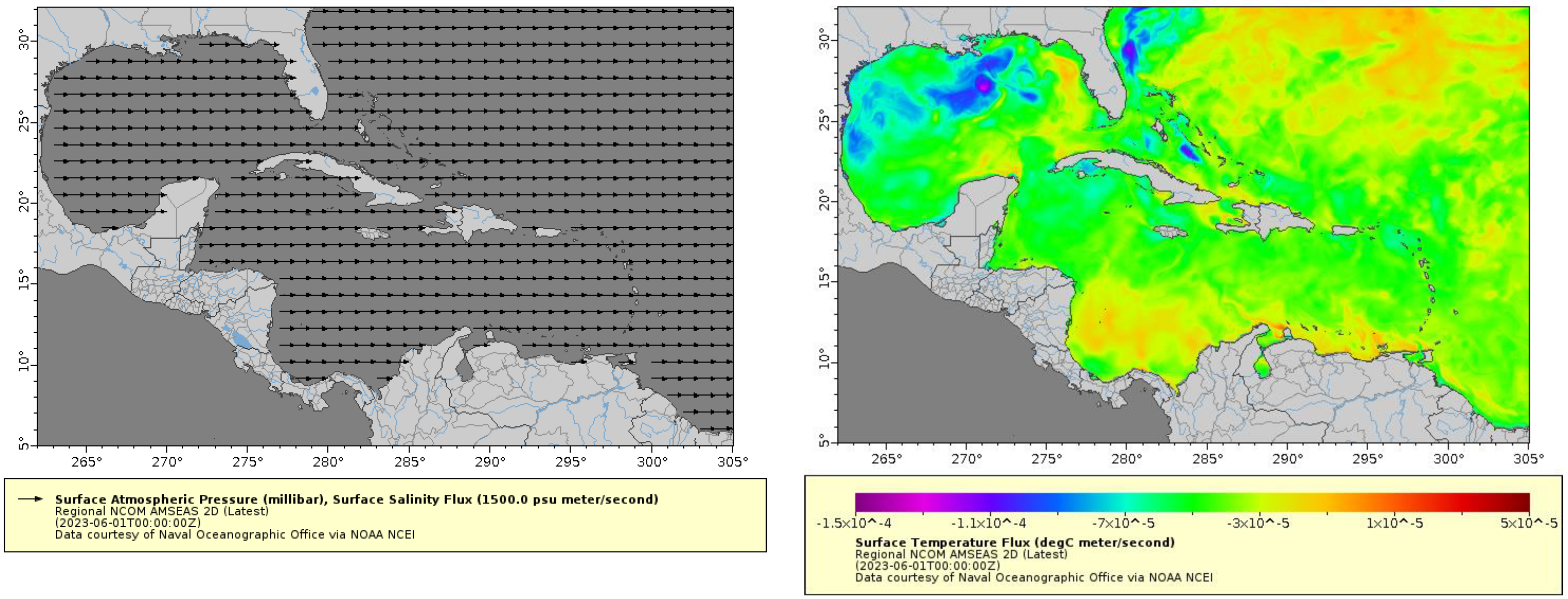
The study dataset includes a large number of observations from 5.0°N–32.1°N and 262.0°E–305.1°E, from 5 April 2013 to the present. The dataset contains several key oceanographic variables for monitoring, including: water surface elevation, surface atmospheric pressure, surface temperature flux, surface salinity flux, surface shortwave flux, surface roughness, eastward surface wind stress, and northward surface wind stress. The source data can be downloaded from the Environmental Research Division’s Data Access Program (ERDDAP) website [26], which provides easy-to-use generation and various common dataset file formats for downloading. The website provides not only tabular data in various common formats, but graphical data, such as maps of the dataset and distribution of environmental parameters, can also be generated.

The environmental variables of the studied area are measured by the recoded values at image pixels. The selected dataset includes data from January 2015 to December 2022. An example of the data sample in this public accessible database are shown in Figure 2.

4. Methods

This section provides the detailed descriptions of the proposed methodology of the study problem. In general, the objective of the proposed method is to reconstruct the image series of a target variable using the image series of a source variable.

For a source variable, suppose $X\in {ℝ}^{H\times W}$ denotes a remote sensing image, where $H$ and $W$ denote the height and width of the image, respectively. For a series of images with time step of T, suppose $\mathbb{X}\in {𝕽}^{H\times W\times T}=\left\{X_1,X_2,\dots ,X_T\right\}$ denote an image series of the source variable. Similarly, suppose $Y\in {𝕽}^{H\times W}$ and $\mathbb{Y}\in {ℝ}^{H\times W\times T}=\left\{Y_1,Y_2,\dots ,Y_T\right\}$ denote an image and image series of a target variable, respectively. The general objective of the cross-variable reconstruction of image series can be defined as follows:

$$Y_1,Y_2,\dots ,Y_T=F\left(X_1,X_2,\dots ,X_T\right).$$

(4)

In this study, the image series of the target variable is iteratively reconstructed using the source variable at each time step, as follows:

$$Y_t=F\left(X_t\right), t=1,2,\dots ,T,$$

(5)

where the function F denotes the proposed deep neural network model for tackling the cross-variable reconstruction problem.

In the following subsections, the developed deep neural network model is introduced in detail, including the proposed convolution and attention feature extractor, the overall neural network structure, and the multivariate time-series loss function.

4.1. Convolution and Attention Feature Extractor

For effective feature extraction, a CAFE network module that consists of the combination of a convolutional layer and an attention layer is proposed. Specifically, the CAFE network module adaptively weighs convolutional weighted features and attentively weighted features as captured representative features. Therefore, the CAFE module is integrated by a convolution layer and an attention layer.

In the convolutional layer, the input $X$ is addressed by a convolutional operator as:

$$H_c=f_c\left(X\right)=W_c\ast X,$$

(6)

where $H_c$ denotes the captured features via convolution, $f_c$ denotes the convolution layer with weight $W_c$, and $\ast$ denotes the convolution operator. In the attention layer, the input $X$ is projected to query matrix $Q=W_{\mathrm{Q}}X$, key matrix $K=W_{\mathrm{K}}X$, and value matrix $V=W_{\mathrm{V}}X$, with weights $W_{\mathrm{Q}}$, $W_{\mathrm{K}}$, and $W_{\mathrm{V}}$, respectively. The attention output is weighed by the corresponding input values through the matrices of query, key, and value. The attention layer is formulated as:

$$\begin{array}{c}{H}_a=f_a\left(X\right)=\phi \left(\frac{1}{d}Q{K}^{\mathrm{T}}\right)\delta \left(V\right)\\ =\phi \left(\frac{1}{d}{W}_{\mathrm{Q}}X{\left(W_{\mathrm{K}}X\right)}^{\mathrm{T}}\right)\delta \left(W_{\mathrm{V}}X\right),\end{array}$$

(7)

where $H_a$ denotes the captured features via attention, $f_a$ denotes the attention layer in the CAFE module, $\phi$ and $\delta$ denote the mapping functions, and T denotes the transpose operation. $Q{K}^{\mathrm{T}}$ indicates the alignment between the query matrix and the key matrix. The alignment result is scaled down by a factor $d$ to avoid the effect of large dot products that may cause abnormal gradients.

Consequently, the convolutional layer and the attention layer are combined under an adaptive weighting mechanism. Particularly, a self-attention mechanism is used to weight the features among the convolutional layer and the attention layer, which is formulated as:

$$H=\mathrm{Concat}\left(\mathsf{\alpha }{H}_a,\beta H_c\right),$$

(8)

where the weights $\mathsf{\alpha }$ and $\beta$ are derived as $\left[\mathsf{\alpha },\beta \right]\in {𝕽}^2=\mathrm{Softmax}\left({\phi }^{\prime }\left(\mathrm{Concat}\left(H_a,H_c\right)\right)\right)$. Thus, Equation (8) can be obtained as:

$$H=\mathrm{Softmax}\left({\phi }^{\prime }\left(\mathrm{Concat}\left(H_a,H_c\right)\right)\right)⨀\mathrm{Concat}\left(H_a,H_c\right)),$$

(9)

${\phi }^{\prime }$ denotes the mapping functions, $⨀$ denotes element-wise dot product.

The structure of the proposed CAFE module is shown in Figure 3. The convolutional layer captures the local correlations within input image data using a convolutional kernel, while the attention layer extracts the driving features within input image data using attention mechanism. Finally, another self-attention mechanism is designed to adaptively weigh the extracted features among the convolution and the attention layers. The next subsection introduces the utilization of the proposed CAFE module.

4.2. CAFE-Based Recurrent Neural Network

The proposed CAFE module is used as the core module of the deep neural network. A series of CAFE mechanisms is embedded and stacked into a recurrent neural network architecture.

To extract the temporal features within the image series, the weighted features of a single image are sequentially input into a recurrent neural network. ConvGRU proposed a hybrid neural network with convolution operation of three-dimensional input embedded into a GRU module [8]. Inspired by ConvGRU, the CAFE module is embedded into a three-dimensional GRU network. The designed CAFE-based GRU is formally defined as follows:

$$\begin{array}{c}{U}_t=\mathrm{Sigmoid}\left(W_u\ast \left[H_{t-1}^l;{\tilde{A}}_t\right]+b_u\right)\\ R_t=\mathrm{Sigmoid}\left(W_r\ast \left[H_{t-1}^l;{\tilde{A}}_t\right]+b_r\right)\\ {\tilde{H}}_t=\mathrm{Tan}\mathrm{h}\left(W_{\mathrm{h}}\ast [R_t⨀H_{t-1}^l;{\tilde{A}}_t]+b_{\mathrm{h}}\right)\\ H_t=\left(1-U_t\right)⨀H_{t-1}^l+U_t⨀{\tilde{H}}_t,\end{array}$$

(10)

where $H_{t-1}^l$ denotes the input matrix of the $l$th stack of time step $t-1$. $H_t^l$ and $C_t^l$, respectively, denote the hidden state matrix and the cell state matrix of the $l$th stack at time step $t$. $\ast$ denotes the convolution operator, and $⨀$ denotes the element-wise multiplication operator. $U_t$ indicates the update gate, and $R_t$ indicates the reset gate. $W$ and $b$, respectively, denote the network weight matrix and the bias matrix for training. At the initial stage, the hidden state matrix and cell state matrix are set to zero matrices, respectively.

The CAFE-based GRU determines the future hidden state by the inputs and past hidden states of its previous neighbors. CAFE-GRU is a hybrid neural network for spatiotemporal representative learning that integrates both convolutional and attention mechanisms in both input-to-state and state-to-state transitions.

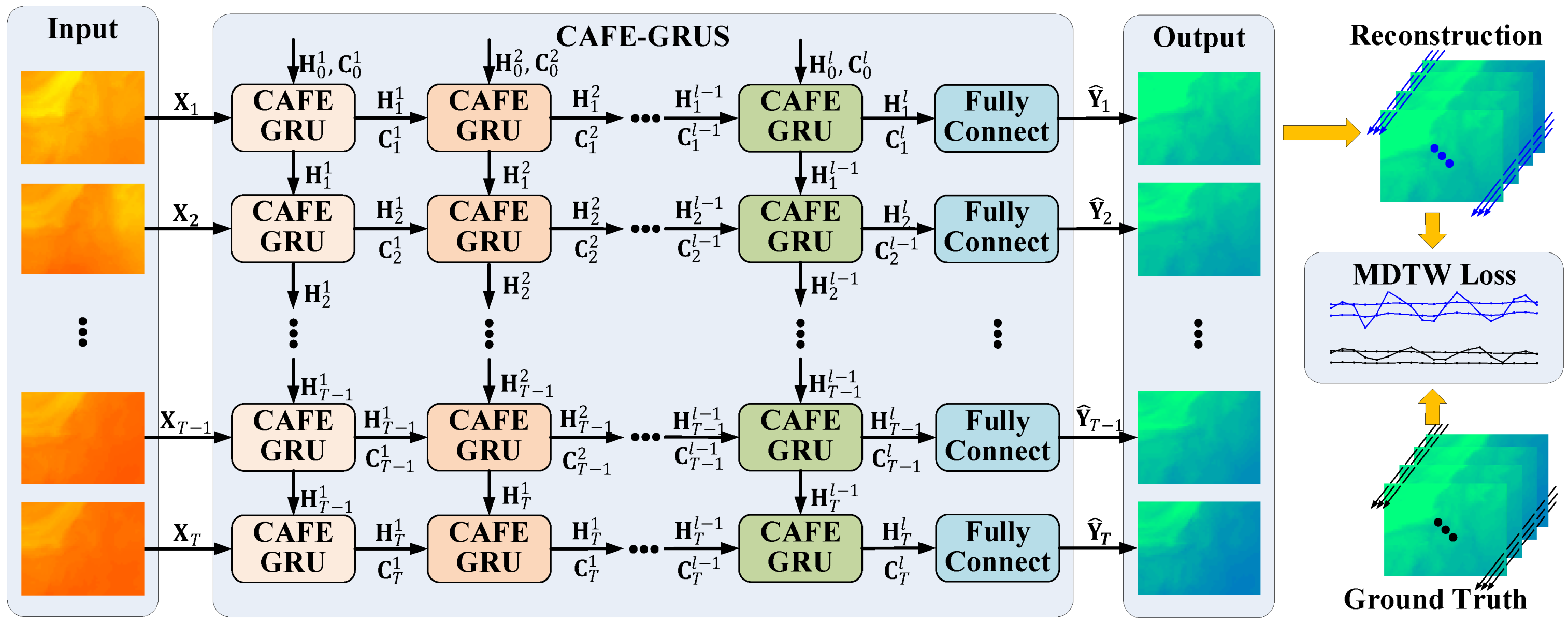
Finally, the reconstruction results of the target variable are generated by fully connected layers, given the generated hidden states at $l$th stack. At time step t, the reconstruction result can be obtained by:

$${\widehat{Y}}_t=\mathrm{FullyConnect}\left(H_t^l\right),$$

(11)

With the above-mentioned process, an image series of the source variable $X_1,X_2,\dots ,X_T$ is sequentially input into the network. A set of CAFE-based GRU modules are stacked to extract the driving features across the source and the target variables in regression. As a result, the reconstructed image series of the target variable ${\widehat{Y}}_1,{\widehat{Y}}_2,\dots ,{\widehat{Y}}_T$ is sequentially output.

The overall architecture of the proposed CAFE-based GRU stacks (CAFE-GRUS) model is shown in Figure 4. As shown in the figure, the proposed CAFE-GRUS model flows in a stacked network structure. The source images are input into the CAFE modules with recurrent stacks, while the last stack of CAFE-GRU modules finally generates the target images over time via fully connected layers.

To train the proposed CAFE-GRUS model, the source image series is addressed as the input, while the target image series is used as the label. The model is trained in an end-to-end manner via supervised learning under a proposed MDTW loss function that is introduced in the next subsection.

4.3. MDTW Loss Function

In general, the traditional DTW algorithm mentioned in Section 2.2 can only deal with one-dimensional time series, and cannot compare the relationship between multi-dimensional time series. Therefore, we propose a loss function that can calculate the correlation degree between multivariate time series, called the multivariate dynamic time warping (MDTW) loss function.

Suppose that there are two n-dimensional time series of $A=\left\{a_1,a_2, \dots ,a_t\right\}$ and $B=\left\{b_1,b_2,\dots ,b_{\tau }\right\}$ which need to be warped, where t and τ are the number of data points of each time series, respectively, and $a_i=\left[a_{i,1},a_{i,2}, \dots ,a_{i,n}\right]$ and $b_j=\left[b_{j,1}{b}_{j,2}, \dots ,b_{j,n}\right]$ represent the data points of the time series. Using the Euclidean rule in space, the Euclidean distance is calculated to characterize the data gap between two time series, and the distance is defined as:

$$d\left(a_i,b_j\right)={{\displaystyle \sum }}_{k=1}^n\sqrt{{\left(a_{i,k}-b_{j,k}\right)}^2}={{\displaystyle \sum }}_{k=1}^n\left|a_{i,k}-b_{j,k}\right|,$$

(12)

Next, the cumulative distance matrix D between the two time series is calculated using the following equation:

$$D\left(i,j\right)=d\left(a_i,b_j\right)+\min \left\{D\left[i-1,j\right],D\left[i,j-1\right],D\left[i-1,j-1\right]\right\},$$

(13)

Considering the high time cost of computing the distance between multidimensional time series, we propose a method to accelerate the calculation of MDTW distance matrix. If two time series are more similar, their shortest paths in MDTW distance matrix are generally closer to the diagonal.

Step 1: We first select the three diagonal strip regions near the diagonal in the distance matrix, i.e., $\left(i,i\right),\left(i,i+1\right),\left(i+1,i\right),i\in \left(0,t\right)$ as MDTW distance first calculation region;

Step 2: After the calculation is completed, we start the shortest path search process in this region. Similar to the traditional DTW, first draw a 2 × 2 distance comparison matrix from $\left(t,\tau \right)$, the minimum value in the distance comparison matrix is used as the starting point for the next drawing of the distance comparison matrix;

Step 3: If the minimum value approaches to the boundary of the MDTW distance first calculation for the first time, i.e., the minimum value appears in $\left(i,i+1\right) \mathrm{or} \left(i+1,i\right)$, then it is necessary to extend a slash strip region outside the boundary, i.e., $\left(i,i+2\right) \mathrm{and} \left(i+2,i\right)$, at which time the region for MDTW distance calculation becomes another extended region;

Step 4: The above shortest path search process continues within the region until the boundary is next touched, and then a similar process of expanding the region outward as described above is carried out until the path reaches (0,0);

Step 5: We get the correspondence, calculate the corresponding distance according to the correspondence, and sum up to get the MDTW distance.

Given the above steps for formulating the MDTW, Figure 5 shows an execution example of MDTW, which shows the process of calculating the shortest path between two groups of multivariate time series using the MDTW algorithm. Figure 5a indicates that the cells of the MDTW distance in a diagonal region are calculated first, and the shortest path is searched within the region. As shown in the figure, the path touches the region boundary at (10,9); at this time, it is necessary to extend a diagonal region to both sides of the region. Subsequently, Figure 5b shows the region of the MDTW distance after the expansion, and the path touches the region boundary again at (2,4), and needs to be expanded again. Then, Figure 5c shows the region after another expansion and, finally, generates the MDTW shortest path.

With the proposed MDTW, the score is utilized as a loss. In other words, the MDTW process is defined as a loss function for training the proposed deep neural network model. The parameters of the model are tuned by minimizing the MDTW loss function to measure the difference between the predicted values and the ground truth values. The MDTW loss is defined as:

$$Loss=\mathrm{MDTW}\left(\widehat{\mathbb{Y}},\mathbb{Y}\right)$$

(14)

where $\widehat{\mathbb{Y}}=\left\{{\widehat{Y}}_1,{\widehat{Y}}_2,\dots ,{\widehat{Y}}_T\right\}$ and $\mathbb{Y}=\left\{Y_1,Y_2,\dots ,Y_T\right\}$ represent the resulting reconstruction and the ground truth label in a training dataset, respectively. $N$ represents the total number of pixels for a prediction at time instance $t$. The Adam optimizer [27] is implemented to train the CAFE-GRUS model under the MDTW loss function.

5. Results

In this section, the experimental results are provided to validate the reconstruction performance of the proposed neural network. The descriptions of the experimental setup, the performance of the proposed and compared methods, and the ablation study results are demonstrated in this section.

5.1. Experimental Setup

Experiments are conducted using the real-world remote sensing dataset that is introduced in Section 3.2. The dataset is split to three subsets as training set, validation set, and testing set. The data from 2015 to 2019 is selected as a training set, while the data from 2020 to 2021 is selected as validation dataset. The data from 2021 to 2022 is used as ground truth to quantitatively evaluate the prediction performance of the proposed algorithm. The number of data samples of each dataset is summarized in

Table 1. Setup of the study dataset in the experiments.

Dataset	Year Range	Sample Number	Percentage
Training	2015–2019	14,202	72%
Validation	2020–2021	2643	13%
Test	2021–2022	2915	15%

.

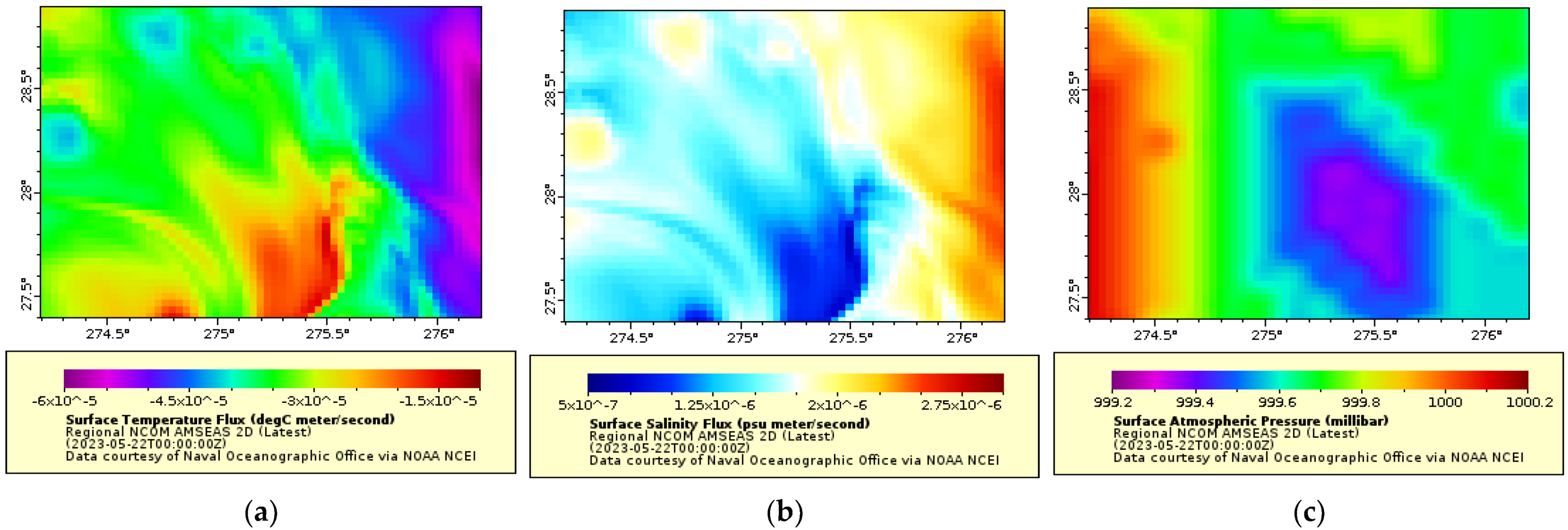
From the dataset, surface temperature flux (STF), surface salinity flux (SSF), and surface atmosphere pressure (SAP) are chosen as the studied environmental variables in the experiments. In addition, the region of North America (27.4°N–28.9°N, 274.2°E–276.2°E) is chosen for experimental evaluation. Records of each environmental field corresponds to an image with 45 × 60 pixel of 2700 pixels in total. The selected area under study involves highly dynamic variations and complex fine-scalar structures of environmental variables. These characteristics make this region an ideal field and a representative testbed for quantitative and qualitative evaluation in the experiments. Examples of data samples are shown in Figure 6.

In the experiments, to avoid the negative effect of different ranges corresponding to the three environmental variables, the data sample of each variable is preprocessed using mean-standard deviation normalization. Both of input and output time windows are set to 5 in the experiments.

Several baseline methods are compared in the experiments to evaluate the performance of the proposed method. These methods are the state-of-the-art methods that have been developed for generating image series of environmental variables. The compared baseline models in the experiments are:

• ResNet: A residual neural network (ResNet) integrates residual functions in weight layers with reference to inputs;
• ConvLSTM: ConvLSTM combines a convolutional layer with a long short-term memory network, which is used for feature extraction and to capture both spatial and temporal dependencies in image series;
• ConvGRU: ConvGRU combines convolutional layers with a GRU network, which is used for feature extraction and to capture both spatial and temporal dependencies in image series;
• CSA-ConvLSTM: A convolutional self-attention (CSA) mechanism is integrated into a ConvLSTM neural network for forecasting environmental image series.

All the compared methods are finely tuned to their best performance in the experiments, for fair comparison.

To assess the reconstruction accuracy, the mean absolute error (MAE) metric is reported to measure the difference between the reconstructed image and the ground truth. Particularly, at any evaluation time $t$ in testing, the MAE metric can be obtained as:

$$e=\frac{1}{T·H·W}{\displaystyle \sum }_{t=1:T}\left|{\widehat{Y}}_t-Y_t\right|$$

(15)

where $e$ evaluates the prediction performance of a data sample. To evaluate the general prediction accuracy on the entire testing set, the above metric is further utilized to perform averaging of MAE over the testing set, which is defined as:

$$\mu =\frac{1}{I}{\displaystyle \sum }_i{e}_i,$$

(16)

where $I$ denotes the total number of data samples in the testing dataset. In addition, the standard deviation of averaging the MAE over the testing set is also used as an evaluation metric, which is defined as:

$$\sigma =\sqrt{\frac{1}{I}{\displaystyle \sum }_i{\left(e_i-\mu \right)}^2},$$

(17)

In the experiments, the proposed and the compared methods are executed using Python 3.8 and Pytorch 1.5 on a desktop PC with the following hardware: an Intel i9-9900K, 16GB of RAM, and an Nvidia RTX 3070 GPU. The experimental results are demonstrated in the following subsection.

5.2. Experimental Results

With the experimental setup that is introduced in Section 5.1, the experiments are conducted accordingly. In the experiments, three environmental variables (Temp, Sali, and Pres) in the dataset are cross validated. Specifically, any two environmental variables are chosen as source and target variables in the experiment. Therefore, there are six cross-variable reconstruction tasks among the three environmental variables, namely: (1) from STF to SSF, (2) from STF to SAP, (3) from SSF to STF, (4) from SSF to SAP, (5) from SAP to STF, and (6) from SAP to SSF.

Table 2. Experimental results of compared and proposed models for cross-variable reconstruction ($\mu \pm \sigma$).

Compared Model	STF to SSF 10−6 Psu-m/s	SSF to STF 10−6 °C-m/s	STF to SAP Pa	SAP to STF 10−6 °C-m/s	SSF to SAP Pa	SAP to SSF 10−6 Psu-m/s
ConvLSTM	10.65 ± 4.03	12.93 ± 6.11	103 ± 26	13.34 ± 6.99	121 ± 32	13.94 ± 7.97
ConvGRU	8.85 ± 2.91	10.32 ± 4.82	94 ± 23	12.93 ± 5.28	98 ± 25	12.39 ± 7.38
ResNet	6.07 ± 2.08	7.99 ± 3.59	78 ± 13	10.32 ± 4.82	89 ± 12	11.42 ± 6.94
CSAResNet	5.68 ± 1.94	7.93 ± 2.73	73 ± 12	8.93 ± 4.32	87 ± 13	9.22 ± 5.20
CAFE-GRUS	3.43 ± 0.91	5.57 ± 1.35	55 ± 6	6.20 ± 3.97	68 ± 8	7.93 ± 4.82

provides the experimental results of the compared and proposed models for cross-variable reconstruction. In the table, the cells provide the results toward the evaluation metrics of $\mu \pm \sigma$. As seen in the table, the proposed model provides the best performance over the six cross-variable reconstruction tasks. Among the tasks, the STF to SSF task demonstrates the best performance compared to the other tasks.

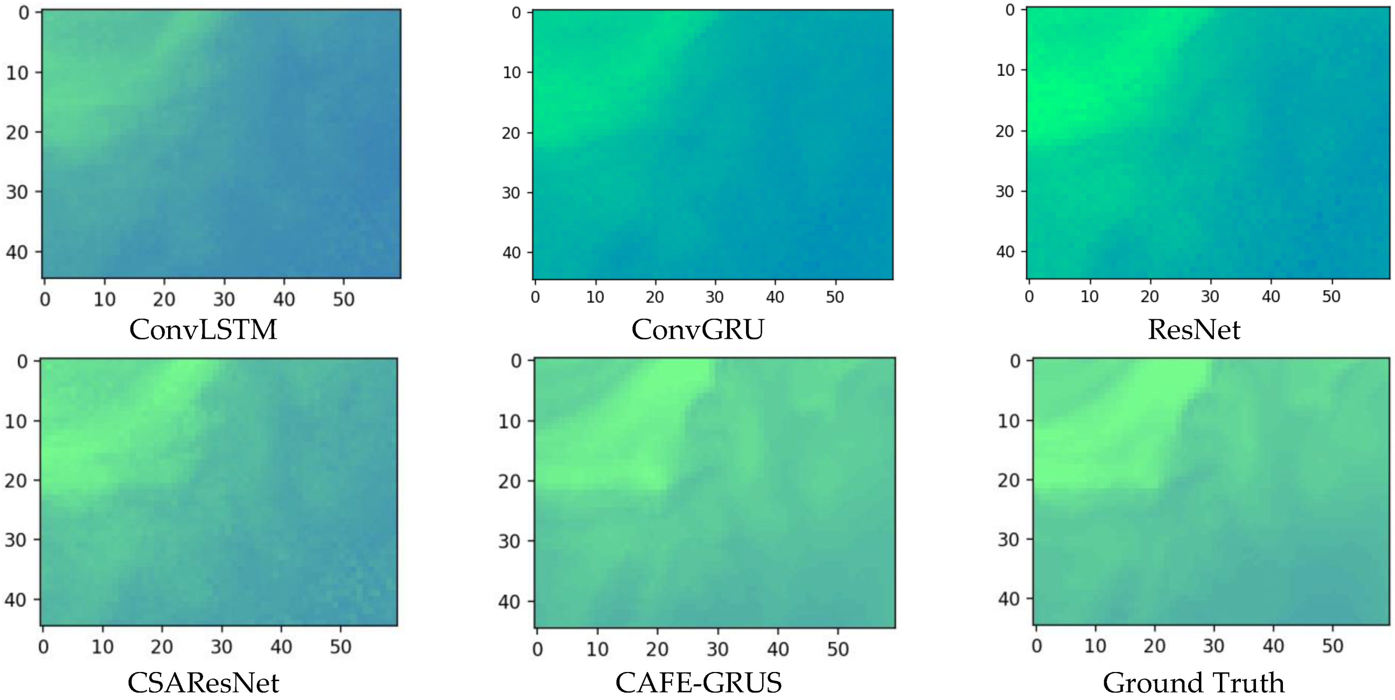
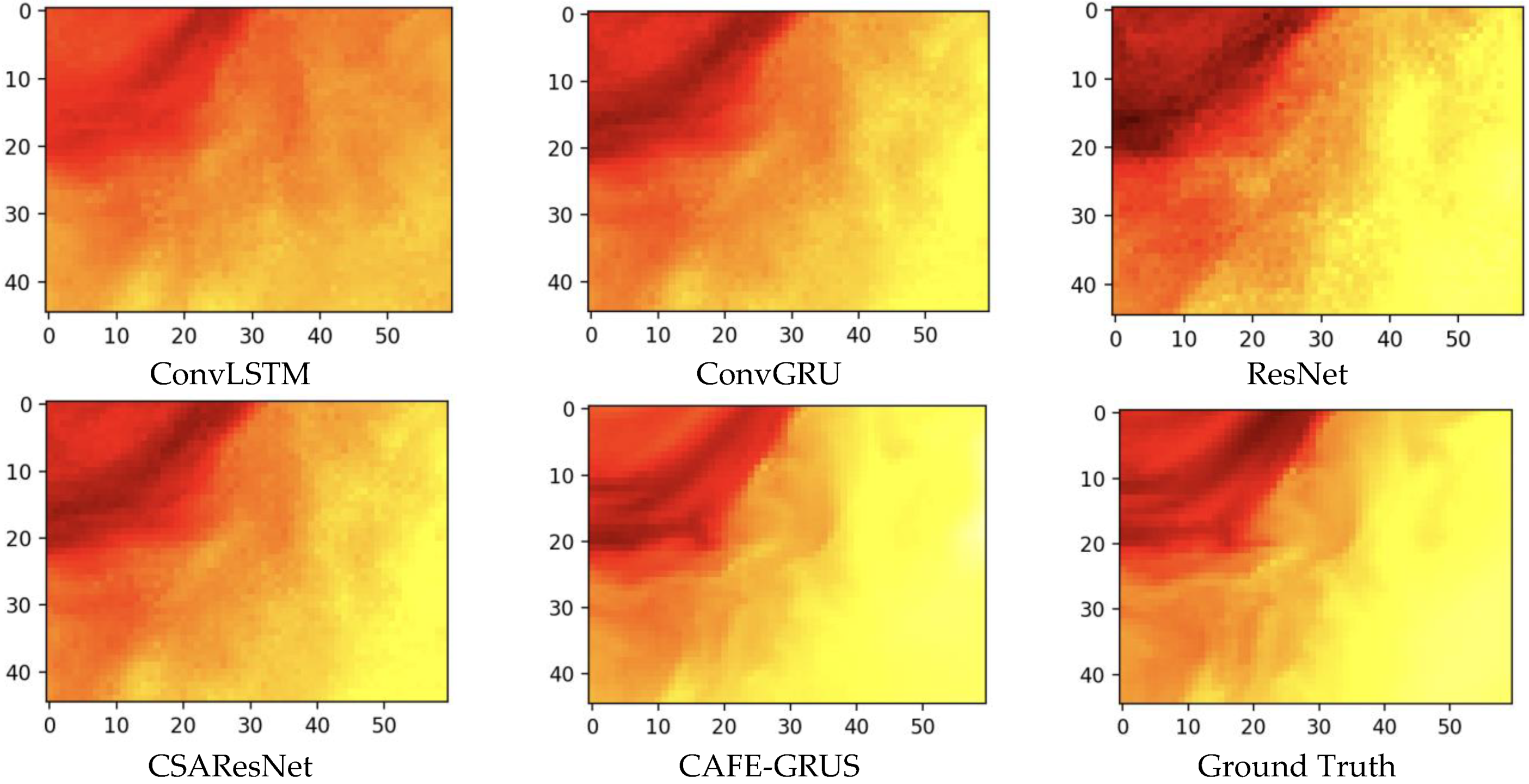
The quality of the reconstructed images mainly depends on the quality of the raw data and the accuracy of the reconstruction model. To clearly demonstrate the reconstruction performance using the proposed CAFE-GRUS model, the reconstructed image series of (1) from STF to SSF and (2) from STF to SAP are chosen for display. The results refer to the reconstructed images at the last time step of the network output. Figure 7 shows examples of the reconstructed images using CAFE-GRUS on STF to SSF task in testing. Figure 8 shows examples of the reconstructed images using CAFE-GRUS on SSF to STF task in testing. As shown in these figures, among all the compared models, the reconstructed images of the proposed model can provide more accurate images compared with the ground truth images. These figures provide the real testing results with visual representation, which can be interpreted towards the algorithm performance.

Furthermore, the reconstruction results of CAFE-GRUS at each time step are considered in the experiments.

Table 3. Experimental results of compared and proposed models for cross-variable reconstruction ($\mu \pm \sigma$).

CAFE-GRUS	STF to SSF 10−6 Psu-m/s	SSF to STF 10−6 °C-m/s	STF to SAP Pa	SAP to STF 10−6 °C-m/s	SSF to SAP Pa	SAP to SSF 10−6 Psu-m/s
Time Step 1	4.11 ± 0.98	5.63 ± 1.55	59 ± 9	6.24 ± 4.32	69 ± 10	8.03 ± 5.12
Time Step 2	3.45 ± 0.92	5.58 ± 1.43	59 ± 7	6.22 ± 3.98	69 ± 9	7.97 ± 4.96
Time Step 3	3.44 ± 0.92	5.59 ± 1.38	55 ± 7	6.21 ± 3.95	66 ± 7	7.99 ± 4.81
Time Step 4	3.40 ± 0.91	5.57 ± 1.38	54 ± 6	6.18 ± 3.95	64 ± 8	7.93 ± 4.82
Time Step 5	3.37 ± 0.88	5.50 ± 1.32	52 ± 5	6.12 ± 3.90	62 ± 7	7.91 ± 4.71

shows the accuracy of the reconstruction over time steps using CAFE-GRUS. The results show the specific reconstruction accuracy with respect to each time step in testing. As can be seen, the error and the standard deviation are relatively similar, which means the reconstruction performance are reliable for each time step. There are only slight differences between steps that the later steps perform slightly better than the former steps. This is because the later ones share more temporal information from the former time steps.

6. Discussion

To determine the component contribution to the overall neural network model, an ablation study is conducted by removing certain components of CAFE-GRUS. The ablation study can evaluate the performance of the proposed components in CAFE-GRUS. The models of the ablation study are configured as:

• ConvGRU: The basic backbone with convolutional and GRU neural network with a loss function of basic mean absolute error;
• ConvGRU with MDTW: The convolutional and GRU neural network with the proposed MDTW loss function;
• CAFE-GRUS: The proposed CAFE-GRUS model with a loss function of basic mean absolute error;
• CAFE-GRUS with MDTW: The full version of the proposed CAFE-GRUS model with the proposed MDTW loss function.

Table 4. Ablation study results of proposed models for cross-variable reconstruction ($\mu \pm \sigma$).

Compared Model	STF to SSF 10−6 Psu-m/s	SSF to STF 10−6 °C-m/s	STF to SAP Pa	SAP to STF 10−6 °C-m/s	SSF to SAP Pa	SAP to SSF 10−6 Psu-m/s
ConvGRU	8.85 ± 2.91	10.32 ± 4.82	94 ± 23	12.93 ± 5.28	98 ± 25	12.39 ± 7.38
ConvGRU with MDTW	6.92 ± 2.19	85 ± 17	11.42 ± 3.97	99 ± 21	10.43 ± 5.85	11.86 ± 7.27
CAFE-GRUS	5.43 ± 1.94	78 ± 14	9.72 ± 3.83	96 ± 19	9.32 ± 5.28	10.53 ± 6.11
CAFE-GRUS with MDTW	3.43 ± 0.91	5.57 ± 1.35	55 ± 6	6.20 ± 3.97	68 ± 8	7.93 ± 4.82

provides the experimental results of all the compared ablation models and the full version of the proposed CAFE-GRUS model. The results show how the network components affect the performance of cross-variable reconstruction. In the table, the best performance is achieved by the full version of CAFE-GRUS. Among the other ablation models, both CRNN with MDTW and CAFE-GRUS outperform the basic backbone model of CRNN. The ablation study results validate the effectiveness of the proposed network components for cross-variable reconstruction. The proposed feature extractor and the loss function enable the recurrent stacks to be trained more accurately, which effectively improve the reconstruction performance.

The proposed model is particularly useful when dealing with large datasets that have missing values or when trying to estimate values for variables that are difficult or expensive to measure directly. This manner can be used in a variety of fields in remote sensing and monitoring programs.

In general applications, image series of remote sensing have been implemented for estimation or prediction using a single environmental variable. This study addresses the problem of image series reconstruction from one source variable to another target variable.

The application of cross-variable reconstruction is used to estimate incomplete data in a dataset by using information from other variables in the same dataset.

7. Conclusions

Image reconstruction of target variables from source variables could provide useful information for environmental monitoring programs. This article introduced a novel deep neural network model that was focused on cross-variable image reconstruction of remote sensing. The proposed model exploited high-resolution images of environmental data through convolutional and spatial attention to learn the relationships between the source and the target data. To demonstrate its performance, experiments on real-world datasets were conducted. The experimental results validate the superior performance of the proposed model for cross-variable reconstruction. The efforts of the proposed model contributed to provide precise reconstruction of environmental image series, leading planners and administrations to make proper decision-making. In the future work, the problem of image reconstruction can be extended to achieve multi-variable reconstruction simultaneously within one deep learning architecture.

References

1. Yuan, Q.; Shen, H.; Li, T.; Li, Z.; Li, S.; Jiang, Y.; Xu, H.; Tan, W.; Yang, Q.; Wang, J.; et al. Deep learning in environmental remote sensing: Achievements and challenges. Remote Sens. Environ. 2020, 241, 111716. [Google Scholar]
2. Zeng, C.; Shen, H.; Zhong, M.; Zhang, L.; Wu, P. Reconstructing MODIS LST based on multitemporal classification and robust regression. IEEE Geosci. Remote Sens. Lett. 2014, 12, 512–516. [Google Scholar] [CrossRef]
3. Zeng, C.; Long, D.; Shen, H.; Wu, P.; Cui, Y.; Hong, Y. A two-step framework for reconstructing remotely sensed land surface temperatures contaminated by cloud. ISPRS J. Photogramm. Remote Sens. 2018, 141, 30–45. [Google Scholar] [CrossRef]
4. Hong, F.; Zhan, W.; Göttsche, F.M.; Liu, Z.; Zhou, J.; Huang, F.; Lai, J.; Li, M. Comprehensive assessment of four-parameter diurnal land surface temperature cycle models under clear-sky. ISPRS J. Photogramm. Remote Sens. 2018, 142, 190–204. [Google Scholar] [CrossRef]
5. Li, J.; Yu, Z.; Yu, L.; Cheng, P.; Chen, J.; Chi, C. A Comprehensive Survey on SAR ATR in Deep-Learning Era. Remote Sens. 2023, 15, 1454. [Google Scholar]
6. Zhang, L.; Zhang, L.; Du, B. Deep learning for remote sensing data: A technical tutorial on the state of the art. IEEE Geosci. Remote Sens. Mag. 2016, 4, 22–40. [Google Scholar] [CrossRef]
7. Hochreiter, S.; Schmidhuber, J. Long short-term memory. Neural Comput. 1997, 9, 1735–1780. [Google Scholar] [CrossRef]
8. Cho, K.; Van Merriënboer, B.; Gulcehre, C.; Bahdanau, D.; Bougares, F.; Schwenk, H.; Bengio, Y. Learning phrase representations using RNN encoder-decoder for statistical machine translation. arXiv 2014, arXiv:1406.1078. [Google Scholar]
9. Shi, X.; Chen, Z.; Wang, H.; Yeung, D.Y.; Wong, W.K.; Woo, W.C. Convolutional LSTM network: A machine learning approach for precipitation nowcasting. Adv. Neural Inf. Process. Syst. 2015, 28, 1–9. [Google Scholar]
10. Shi, X.; Gao, Z.; Lausen, L.; Wang, H.; Yeung, D.Y.; Wong, W.K.; Woo, W.C. Deep learning for precipitation nowcasting: A benchmark and a new model. Adv. Neural Inf. Process. Syst. 2017, 30, 1–11. [Google Scholar]
11. Malek, S.; Melgani, F.; Bazi, Y.; Alajlan, N. Reconstructing cloud-contaminated multispectral images with contextualized autoencoder neural networks. IEEE Trans. Geosci. Remote Sens. 2017, 56, 2270–2282. [Google Scholar] [CrossRef]
12. Zhang, Q.; Yuan, Q.; Zeng, C.; Li, X.; Wei, Y. Missing data reconstruction in remote sensing image with a unified spatial–temporal–spectral deep convolutional neural network. IEEE Trans. Geosci. Remote Sens. 2018, 56, 4274–4288. [Google Scholar] [CrossRef] [Green Version]
13. Li, T.; Gu, Y. Progressive spatial–spectral joint network for hyperspectral image reconstruction. IEEE Trans. Geosci. Remote Sens. 2021, 60, 1–4. [Google Scholar] [CrossRef]
14. Zhang, W.; Li, J.; Hua, Z. Attention-based tri-UNet for remote sensing image pan-sharpening. IEEE J. Sel. Top. Appl. Earth Obs. Remote Sens. 2021, 14, 3719–3732. [Google Scholar] [CrossRef]
15. Ebel, P.; Xu, Y.; Schmitt, M.; Zhu, X.X. SEN12MS-CR-TS: A remote-sensing data set for multimodal multitemporal cloud removal. IEEE Trans. Geosci. Remote Sens. 2022, 60, 1–4. [Google Scholar] [CrossRef]
16. Bellman, R.; Kalaba, R. On adaptive control processes. IRE Trans. Autom. Control. 1959, 4, 1–9. [Google Scholar] [CrossRef]
17. Fan, L.; Yang, J.; Sun, X.; Zhao, F.; Liang, S.; Duan, D.; Chen, H.; Xia, L.; Sun, J.; Yang, P. The effects of Landsat image acquisition date on winter wheat classification in the North China Plain. ISPRS J. Photogramm. Remote Sens. 2022, 187, 1–13. [Google Scholar] [CrossRef]
18. Lu, F.; Chen, B.; Zhou, X.D.; Song, D. STA-VPR: Spatio-temporal alignment for visual place recognition. IEEE Robot. Autom. Lett. 2021, 6, 4297–4304. [Google Scholar] [CrossRef]
19. Cai, X.; Xu, T.; Yi, J.; Huang, J.; Rajasekaran, S. Dtwnet: A dynamic time warping network. Adv. Neural Inf. Process. Syst. 2019, 32, 2–11. [Google Scholar]
20. Cuturi, M.; Blondel, M. Soft-dtw: A differentiable loss function for time-series. In Proceedings of the International Conference on Machine Learning PMLR, New York, NY, USA, 20–22 April 2017; pp. 894–903. [Google Scholar]
21. Rath, T.M.; Manmatha, R. Lower-bounding of dynamic time warping distances for multivariate time series. Univ. Mass. Amherst Tech. Rep. MM 2002, 40, 1–4. [Google Scholar]
22. Shokoohi-Yekta, M.; Hu, B.; Jin, H.; Wang, J.; Keogh, E. Generalizing DTW to the multi-dimensional case requires an adaptive approach. Data Min. Knowl. Discov. 2017, 31, 1–31. [Google Scholar] [CrossRef] [PubMed] [Green Version]
23. Zhang, X.; Gao, Y.; Lin, J.; Lu, C.T. Tapnet: Multivariate time series classification with attentional prototypical network. In Proceedings of the AAAI Conference on Artificial Intelligence, Online, 3 April 2020; Volume 34, pp. 6845–6852. [Google Scholar]
24. Shen, D.S.; Chi, M. TC-DTW: Accelerating multivariate dynamic time warping through triangle inequality and point clustering. Inf. Sci. 2023, 621, 611–626. [Google Scholar] [CrossRef]
25. Li, H.; Wan, J.; Liu, S.; Sheng, H.; Xu, M. Wetland Vegetation Classification through Multi-Dimensional Feature Time Series Remote Sensing Images Using Mahalanobis Distance-Based Dynamic Time Warping. Remote Sens. 2022, 14, 501. [Google Scholar] [CrossRef]
26. The Regional NCOM AMSEAS 2D Dataset. Available online: https://www.ncei.noaa.gov/erddap/griddap/NCOM_amseas_latest2d.html (accessed on 22 May 2023).
27. Kingma, D.P.; Ba, J. Adam: A method for stochastic optimization. arXiv 2014, arXiv:1412.6980. [Google Scholar]
Figure 1. An execution example of the DTW process for univariate time series. (a) Corresponding data points of two time series, (b) heat map and the generated shortest path (the green line).
Remotesensing 15 03552 g001
Figure 2. Study field of interest and data examples. The gray arrow area in the left figure indicates the study area, while the color area in the right figure indicates the surface temperature flux [26].
Remotesensing 15 03552 g002
Figure 3. The structure of the proposed convolution and attention feature extractor.
Remotesensing 15 03552 g003
Figure 4. The overall architecture of the proposed neural network model. The architecture achieves the cross-variable feature extraction and field reconstruction.
Remotesensing 15 03552 g004
Figure 5. The execution example of the proposed MDTW process. (a) Initial diagonal region, (b) expanded diagonal region, (c) final MDTW shortest path.
Remotesensing 15 03552 g005
Figure 6. Examples of data samples in the dataset. (a) Surface temperature flux, (b) surface salinity flux, (c) surface atmospheric pressure [26].
Remotesensing 15 03552 g006
Figure 7. Reconstruction results using the compared and proposed models on STF to SSF task.
Remotesensing 15 03552 g007
Figure 8. Reconstruction results using the compared and proposed models on SSF to STF task.
Remotesensing 15 03552 g008