Article

Investigation of Temperature Effects into Long-Span Bridges via Hybrid Sensing and Supervised Regression Models

1
Department of Civil and Environmental Engineering, Politecnico di Milano, Piazza L. da Vinci 32, 20133 Milano, Italy
2
Finnish Meteorological Institute (FMI), Erik Palménin Aukio 1, FI-00560 Helsinki, Finland
*
Author to whom correspondence should be addressed.
Remote Sens. 2023, 15(14), 3503; https://doi.org/10.3390/rs15143503
Submission received: 9 May 2023 / Revised: 27 June 2023 / Accepted: 4 July 2023 / Published: 12 July 2023
(This article belongs to the Special Issue Remote Sensing and SAR for Building Monitoring)

Abstract

:
Temperature is an important environmental factor for long-span bridges because it induces thermal loads on structural components that cause considerable displacements, stresses, and structural damage. Hence, it is critical to acquire up-to-date information on the status, sustainability, and serviceability of long-span bridges under daily and seasonal temperature fluctuations. This paper intends to investigate the effects of temperature variability on structural displacements obtained from remote sensing and represent their relationship using supervised regression models. In contrast to other studies in this field, one of the contributions of this paper is to leverage hybrid sensing as a combination of contact and non-contact sensors for measuring temperature data and structural responses. Apart from temperature, other unmeasured environmental and operational conditions may affect structural displacements of long-span bridges separately or simultaneously. For this issue, this paper incorporates a correlation analysis between the measured predictor (temperature) and response (displacement) data using a linear correlation measure, the Pearson correlation coefficient, as well as nonlinear correlation measures, namely the Spearman and Kendall correlation coefficients and the maximal information criterion, to determine whether the measured environmental factor is dominant or other unmeasured conditions affect structural responses. Finally, three supervised regression techniques based on a linear regression model, Gaussian process regression, and support vector regression are considered to model the relationship between temperature and structural displacements and to conduct the prediction process. Temperature and limited displacement data related to three long-span bridges are used to demonstrate the results of this research. The aim of this research is to assess and realize whether contact-based sensors installed in a bridge structure for measuring environmental and/or operational factors are sufficient or if it is necessary to consider further sensors and investigations.

1. Introduction

Bridges are vital civil structures that play significant roles in transportation, social life, and economics. During their long-term service life, bridges may be subjected to various unpredictable excitation sources such as earthquakes, wind, floods, typhoons, etc. Apart from such conditions, temperature is an important environmental factor that can induce considerable loads to bridge structures and cause large displacements or deformations. To preserve such vital structures from any type of irreparable damage and undesirable serviceability, structural health monitoring (SHM) has emerged in civil engineering. This technology aims to provide a practical process for continuously monitoring civil structures, particularly bridges [1,2,3,4,5], and to warn of any abnormal event caused by any source of excitations.
Due to advancement in sensing technology, computer systems, and computational techniques, particularly in the field of artificial intelligence, an SHM strategy is often implemented under machine learning algorithms [6,7]. In this regard, it suffices to measure raw structural responses through various sensors, store and transmit measured data, extract meaningful information/features (i.e., feature extraction), and apply machine learning methods for decision-making (i.e., classification, regression, prediction, anomaly detection, etc.). Sensing technology is an important part of an SHM strategy [8,9]. The classical sensing techniques concentrate on contact sensors (e.g., accelerometers, strain gages, fiber optic sensors, temperature sensors, anemometers, etc.) with the aids of wired or wireless data transformation systems. In addition to this technology, the measurement of structural responses can be implemented by next-generation sensors via devices such as digital cameras, video cameras, high-speed cameras, and smartphones [10]. The major goal of this technology is to provide optical images and videos and to extract structural responses (e.g., displacements).
Despite the applicability of both contact and non-contact sensing systems, it is not always trivial to utilize them, especially in long-term SHM programs on large structures, due to recording and storing massive SHM data and the limitation of a dense sensor network for capturing all possible conditions. Recently, the technology of spaceborne remote sensing via synthetic aperture radar (SAR) images from satellites has received increasing attention among civil engineers for SHM applications [11,12,13,14,15,16,17]. The main objective of this technology is to prepare SAR images from a satellite (e.g., COSMO-SkyMed, TerraSar-X, Sentinel-1) and utilize interferometric synthetic aperture radar (InSAR) techniques [18] in order to extract displacement data as the main structural responses/features from target points marked on the structure. The great advantage of the SAR-based SHM is the possibility of obtaining prior information or archived images of civil structures regarding their initial or normal conditions. The other benefit of this strategy is to measure sufficient structural responses in terms of small data for a long-term monitoring program. Furthermore, it is feasible to cover a wide area of the earth and a huge structure (e.g., dams and long-span bridges) without considering a dense sensor network.
Apart from the structural responses, it is possible to measure some important environmental data such as temperature, humidity, and wind speed and direction by some contact-based sensors [19]. In fact, the feasibility of the measurement of environmental data is a great advantage of the contact-sensing technique. Using such measurements, one can gain deep realization into the relationship between the structural responses and environmental conditions. One of the significant challenges in long-term SHM is the influence of temperature on long-span bridges. This is because such an environmental factor changes daily and seasonally, in which case temperature variability may induce thermal loads on the bridges, leading to large displacements/deformations and undesirable stresses [20]. Thermal loads can cause cracking if the structure or structural part is restrained from movement (e.g., clamped boundary conditions). Accurate thermal load values must therefore be used in bridge design based on knowledge of the actual temperature distribution in the bridge. On the other hand, among all environmental variability cases, it has been proven that daily and seasonal temperature fluctuations have the highest influences on the structural properties [21,22]. An important effect of thermal loads is that they can influence long-span structures when operating normally or even when closed to traffic. This means that, in contrast to other excitation loads such as earthquakes, typhoons, etc., the thermal loads are applied to the bridge permanently. In particular, large-scale and long-span bridge structures in open environment are often subjected to periodically time-varying solar radiation and unceasing structural heat exchange. For these reasons, it is indispensable to investigate structural performance and behavior under temperature effects.
Studies on temperature effects are often conducted under three categories: (1) correlation analysis between structural responses (i.e., displacements, modal data, etc.) and temperature, (2) modeling the relationship between structural response and temperature data, and (3) residual extraction in terms of data normalization. In the first category, one attempts to determine the rate of correlation or dependence between the temperature and structural responses [23,24]. The main requirement for this process is to measure the environmental data (temperature) and utilize a correlation measure. The correlation analysis allows us to deeper realize the main reasons for structural changes. A high correlation means that temperature or thermal loads are the key structural variability. In contrast, a low correlation indicates that other unmeasured environmental or excitation conditions affect the structure. However, the major challenge in this process is the poor performance of linear correlation measures for correctly representing the nonlinear correlation between temperature and structural responses such as modal frequencies. Accordingly, one of the issues considered in this paper is to introduce a nonlinear correlation measure.
The second category is the primary step of the residual analysis and data normalization. In this process, one needs to model the relationship between the temperature and structural responses. Due to the measurement of temperature data, supervised regression techniques are the most appropriate choices [25]. Finally, the third category exploits the outputs of the previous steps in order to remove temperature-induced effects from structural responses and provide normalized data insensitive to environmental (temperature) variability. In the context of SHM, this strategy is called data normalization [26]. One of the important merits of this process is to provide valuable information sensitive to structural properties. On this basis, any change in the normalized structural responses can be interpreted as damage. Data normalization is dependent on the possibility of measuring environmental and/or operational data, which is decomposed into input-output (supervised) [27,28] and output-only (unsupervised) [29,30,31,32,33] algorithms, for which the terms “input” and “output” refer to the environmental (e.g., temperature) and structural response data, respectively.

1.1. Related Works and Challenges

The influence of temperature variability on large-scale structures is a critical issue in SHM. This issue relates to two important facts. First, daily and seasonal temperature fluctuations can produce thermal loads, which can cause critical structural responses. Second, the temperature changes can lead to variability in structural responses and such changes may mistakenly interpreted as damage, which is known as a false-positive error [34]. In some cases, such as freezing weather, the intensity of variability in structural responses is significantly larger than conditions caused by damage [32]. Therefore, it is indispensable to study the effect of temperature on the structural responses of large-scale structures, such as long-span bridges, in numerical studies [35,36,37] and through experimental and field monitoring data [38,39,40,41].
Having considered the strong influences of temperature and thermal loads on structural responses, modeling of the temperature and structural responses can provide deep insights into structural behavior, as well as comprehensive understanding of the temperature distribution and its variability in civil structures and the development of their design, maintenance, and rehabilitation procedures. For these purposes, supervised regression methods provide tried-and-tested algorithms. These methods can not only model the relationship between any environmental/operational condition and structural responses but also implement the problem of prediction. Having considered some dynamic features, such as modal frequencies and strains, the commonly used supervised regression techniques for modeling and prediction include some non-parametric regressors such as multiple regression models [23,42,43] and elaborate parametric regressors, such as various artificial neural networks (ANNs) [25,44], support vector regression (SVR), regression trees, and random forests [25,45].
Despite the considerable studies on modeling the temperature and structural responses from contact-based sensing systems and well-known structural features such as modal frequencies, one of the main shortcomings in this field relates to the scarce research using new structural responses such as displacement data acquired from remote-sensing technology. Huang et al. [46] studied the influences of the ambient temperature on limited displacement samples from 29 SAR images of Sentinel-1 on a long-span bridge. In their research, the authors only applied linear regression models to measure the correlation between the displacement and temperature data. Qin et al. [47] investigated the temperature variations in limited displacement points from SAR images of COSMO-SkyMed and Sentinel-1 on a steel arch bridge. Similarly, linear regression models were used to perform the correlation analysis between the displacement and temperature data. Apart from such little research on the important field of temperature effects on structural responses, the other shortcoming is related to the problem of limited data for regression modeling and prediction. It is well known that SAR-based SHM is a process performed with small or limited data compared to other SHM projects [12], especially those based on contact-based sensing systems.
Finally, the major challenge in long-term SHM via remote sensing is the influences of other unmeasured environmental and/or operational factors. Although the equipment of long-span bridges with various contact-based sensors for measuring different environmental and/or operational factors (e.g., temperature, humidity, wind speed and direction, traffic, etc.) is prevalent [48,49,50], some restrictions, such as total costs, difficulties in data measurement, transmission, and management, sensor malfunctions, etc., can make it unattainable to measure all environmental and/or operational parameters. Under such circumstances, the use of supervised regression models with insufficient predictor data (inputs) may be problematic with erroneous results. Therefore, this research intends to investigate whether bridge structural behavior and responses in conjunction with the remote-sensing technology are influenced by measured environmental factor (i.e., temperature in this study) or other unmeasured environmental and/or operational conditions are influential. In simple terms, this research enables us to find whether the environmental/operational sensors installed in a bridge structure are adequate or whether it is necessary to use further sensors and information.

1.2. Objectives

This paper focuses on three main categories to address some major challenges related to long-term SHM and to enhance this process using hybrid sensing as a combination of contact and spaceborne remote sensors. The three categories include (1) determining the correlation between the temperature and limited displacement data obtained from SAR images, (2) modeling the structural responses under temperature variability and thermal loads by supervised regression methods and then predicting the SAR-based displacement data, and (3) analyzing whether temperature sensors are sufficient or whether the bridge structure under study needs further contact-based sensors for measuring other environmental and/or operational conditions or additional investigations related to the probability of existence of damage. For the first category, the correlation analysis began using a linear measure the Pearson linear correlation coefficient. In the case of nonlinear correlation between the temperature and structural responses, such linear measure may fail in correctly estimating the correlation patterns. To address this drawback, this paper investigates the use of the Spearman correlation coefficient, Kendall correlation coefficient, and the maximal information criterion (MIC), all suitable for nonlinear cases. Regarding the second category, three supervised regression techniques, including a linear regression model (LRM), Gaussian process regression (GPR), and support vector regression (SVR), were applied to model the relationship between the temperature and limited displacement data. Since GPR and SVR are parametric algorithms, Bayesian hyperparameter optimization was considered to optimize the main hyperparameters of these models. Once the supervised regression models were established, the limited displacement data retrieved from a few SAR images were predicted through the single predictor data (i.e., temperature records). The third category involves the installed contact-based sensors in the bridge structure. In essence, it reflects the outputs of the previous two categories. If there is a correlation between the temperature and displacement data or a supervised regression method yields a high prediction (regression) accuracy, one can realize that the environmental/operational sensors (i.e., temperature sensors in this research) installed in the structure are sufficient, and other contact-based sensors are unnecessary for structural behavior assessment and displacement monitoring. In contrast, if there is not a correlation or the supervised regression method fails in yielding a high prediction accuracy, one can conclude that the environmental/operational sensors are insufficient, and it is necessary to install further sensors for measuring other environmental and/or operational conditions. In this case, an early damage assessment may be needed to determine whether the poor correlation is caused by damage. For the verification of the three categories, three kinds of long-span bridge structures with limited displacement data from well-known satellites (i.e., COSMO-SkyMed, TerraSar-X, and Sentinel-1) were considered to conduct this study.

1.3. Contributions

The major contributions of this research can be summarized as: (1) performing a comprehensive study on the influence of temperature variability on limited displacement data of some real-world long-span bridges via various approaches, (2) leveraging the idea of hybrid sensing by two different sensing techniques, (3) using nonlinear correlation measures for cases when there is a nonlinear relationship between temperature and displacement data, and (4) making a decision on the sufficiency of contact-based sensors for measuring the single environmental factor, i.e., temperature. In relation to the first contribution, this paper incorporates three steps of correlation analysis, supervised regression models for representing the relationship between the temperature and displacement data, and prediction. Compared to most of the research studies focusing on modal data identified from acceleration time histories, limited displacement samples extracted from SAR images were utilized to evaluate the thermal effects on long-span bridges. One of the great advantages of the correlation analysis is that it allows us to realize whether the temperature is the dominant variability factor or whether other environmental and/or operational factors affect structural responses (displacement data). Regarding the second contribution, the key novel part of this research is to leverage two kinds of sensing techniques, including contact-based temperature sensors for recording temperature variability and non-contact remote sensors in satellites and SAR images for structural displacement data. For the third contribution, the proposed MIC measure, in addition to the Spearman and Kendall correlation coefficients, can deal with the limitation of the linear correlation coefficient for determining the nonlinear correlation pattern between the temperature and displacement data.

2. Long-Span Bridges

2.1. Dashengguan Bridge

This civil structure is a long-span high-speed railway steel bridge that crosses over Yangtze River in Nanjing, China. Figure 1a shows an actual image of this bridge. The construction of this structure began in 2006 and ended in 2010 to handle a speed of 300 km/h. The bridge consists of a large-span continuous steel arch truss with a total length of 1615 m. This research considers the six main parts of the bridge with the total length of 1272 m (i.e., 108, 192, 336, 336, 192, and 108 m) as depicted in Figure 1b. These parts are separated by seven piers (Piers #4–10) mounted on deep piles. The two main spans over the major navigation channels of the Yangtze River are steel arch trusses with lengths of 336 m and a maximum height of 74 m. The non-curved parts of the bridge have a constant height of 16 m [46]. The arches are comprised of three truss planes above the deck. The main truss has a welded, monolithic joint. The members and gusset plates were welded together in the fabrication yard and then transported to the site and spliced outside the joint with high-strength bolts.
For the investigation of the temperature effects, this paper utilized limited displacement samples extracted from 29 SAR images of Sentinel-1A acquired between 25 April 2015 and 5 August 2016. Indeed, these samples were obtained from the research by Huang et al. [46] based on the persistent scatterer interferometry (PSI) technique for extracting the displacement data on the six piers (i.e., Piers #4–6 and #8–10) by determining the light-of-sight (LOS) deformation time series. Moreover, some contact-based temperature sensors were installed in the bridge to record temperature data during the monitoring time. Figure 2a shows the 29 displacement samples (i.e., in the unit of mm) at the six pier locations, and Figure 2b indicates their corresponding air temperature (°C).

2.2. Lupu Bridge

This civil structure is a steel arch bridge that crosses the Huangpu River in Shanghai, China. Construction of this bridge began in 2000, and the bridge opened to traffic in 2003. Figure 3a shows an actual image of the Lupu Bridge. The main bridge structure has a total length of 750 m, including two side spans of 100 m and a main span of 550 m, as shown in Figure 3b. The girder in the side span (i.e., above the arch rib) is a closed steel box with a width of 41 m and a height of 2.7 m. The box-girder is fixed with the arch ribs, columns, and an end crossbeam of the side spans. The girder of the main span is an open steel box-beam including double main box-girders connected by open crossbeams. The width and height of the main span girder are 39.5 m and 2.7 m, respectively. The girder of the main span is supported on the arch rib by suspenders and connected to the integral arch and girder segment of the side span by bearings at the two ends. In order to balance the huge horizontal thrust of the main span, strong horizontal cables were placed between the two ends of both side span arches. The stiffening girders are supported either directly on the arch rib or by columns from below or by suspenders from above. The stiffening girders of the side spans are fixed with the ribs of the side arch and main arch, while the girder of the main span is supported with sliding bearings on the crossbeams at the intersections of the arch rib and girder.
Due to the sensitivity of the Lupu Bridge to geological and environmental conditions, a SAR-based SHM strategy was carried out to extract displacements of the main span and dome using 38 Stripmap images of TerraSAR-X between 2013 and 2016 [47]. Figure 4a,b indicates the displacement samples of the bridge dome and its main span, respectively. Some contact-based temperature sensors were also considered to record temperature data during the monitoring period. Figure 4c illustrates the recorded temperature data utilized in this paper obtained from the research by Qin et al. [47].

2.3. Rainbow Bridge

This civil structure is a long-span concrete-filled steel tubular arch bridge in Tianjin, China. The bridge was built in 1996 and then opened to traffic at the end of 1998. Figure 5a shows an actual image of the Rainbow Bridge. The total length of this bridge corresponds to 1215.69 m, while the main bridge structure contains three spans with lengths of 164, 168, and 164.7 m, with a width of 32 m. The structure of the Rainbow Bridge includes a rigid arch system with a simple supported down-bearing flexible tie rod. The upper and lower chords along with the arch skewback are filled with micro-expansive concrete. There are eight K-shape transverse bracings of each span. Each arch contains 18 pairs of suspenders with a spacing of 8.3 m, and each suspender is composed of 91 galvanized prestressed steel wires. The deck system consists of prestressed concrete middle cross girder, reinforced concrete T-shaped stiffened longitudinal girder, and T-shaped longitudinal girder [51].
Due to the long-term passage of overweight vehicles for exceeding the design load, serious damage patterns have affected the performance and serviceability of the Rainbow Bridge. Hence, some cracks were detected at a longitudinal concrete beam of the bridge, which caused varying levels of damage in the two adjacent longitudinal concrete beams. In the following, all longitudinal concrete beams were replaced to increase the bridge structural performance and to avoid any catastrophic events such as failure and collapse. A long-term SAR-based SHM study was implemented by Qin et al. [47] to use 53 SAR images from Sentinel-1A between 2015 and 2017. Figure 6a,b illustrates the displacement samples in Piers 1–4 and Spans 1–3, respectively. Moreover, Figure 6c displays the temperature records during the monitoring time. It should be pointed out that a multi-temporal DInSAR technique was incorporated to extract the displacement data. The temperature values were measured by a contact-based sensor on the bridge.

3. Correlation Analysis

The initial step after measuring the environmental data and structural responses is to detect the relationship between them. The great advantage of this process is that one can determine whether the measured environmental data affects the structural responses, or whether the other environmental condition or even damage leads to changes in the structural responses. This strategy also helps us to find the most appropriate data normalization technique for removing the environmental and environmental effects. Accordingly, the measured temperature data acquired from contact-based sensors, along with limited displacement samples from some SAR images, were considered to find their relationships. For this purpose, the most effective and efficient choice was to exploit non-parametric correlation analysis methods.
In statistics, correlation analysis is a statistical technique to measure the strength of the relationship between two variables and compute their association. Simply speaking, this technique computes the level of change in one variable due to the change in the other one. A high correlation level indicates a strong relationship between the two variables, while a low correlation means that the variables are weakly associated. Pearson’s linear correlation coefficient is the most used technique for correlation analysis due to its simplicity and efficiency. Pearson’s correlation coefficient is defined as the covariance of two variables divided by the product of their standard deviations. For the two variables (vectors) x and y with n data points, the sample version of the Pearson’s linear correlation coefficient is given by:
ρ = i = 1 n x i x ¯ y i y ¯ i = 1 n x i x ¯ 2 i = 1 n y i y ¯ 2 1 2
where x ¯ and y ¯ denote the means of the vectors x and y, respectively. The values of ρ vary in the range from −1 to 1, where −1 and 1 represent perfect linear negative and positive correlations. Moreover, in the case of independence of the two variables, ρ = 0, but the vice versa is not necessarily true. The Spearman correlation coefficient is a non-parametric rank-based measure of correlation that aims to measure the strength of association between two variables. In contrast to the Pearson linear correlation coefficient, the Spearman correlation assesses linear and non-linear relationships between the variables x and y. In addition, in the absence of the Pearson coefficient (which has problems of existence linked to the existence of the second-order moments of the variables x and y), the Spearman coefficient always exists [52], according to Salvadori et al. (2007). Equation (2) provides the sample version of the Spearman correlation coefficient:
ρ S = 1 6 δ 2 n n 2 1
where δ denotes the difference between the rank of the variables (vectors) x and y. Similar to the Pearson correlation coefficient, ρ S can range from −1 to 1, where the former indicates a perfect negative correlation, and the latter refers to a perfect positive correlation. In addition, in the case of the independence of the two variables, ρ S = 0, but the vice versa is not necessarily true. Similarly to the Spearman coefficient, the Kendall correlation coefficient is a non-parametric rank-based measure of correlation. In addition, the Kendall coefficient always exists. Given the vectors x and y with n data points, the sample version of the Kendall’s correlation coefficient is given by:
τ = 2 K n n 1
where
K = i = 1 n 1 j = i + 1 n ξ x i , x j , y i , y j
and
ξ x i , x j , y i , y j = 1 i f x i x j y i y j > 0 0 i f x i x j y i y j = 0 1 i f x i x j y i y j < 0
Similarly, the Kendall coefficient ranges from −1 to 1. A value of −1 implies a perfect negative relationship, while a value of 1 indicates that the two variables have a perfect positive association. In the case of the independence of the two variables, τ = 0, but the vice versa is not necessarily true. It should be pointed that, in the absence of the Pearson correlation coefficient, the Kendall and Spearman correlation coefficients assess the statistical associations based on the ranks of datasets.
One of the main drawbacks of the Pearson linear correlation coefficient is related to measuring only the linear correlation between two variables. To address this limitation, Reshef et al. [53] proposed the idea of MIC. This technique is a non-parametric measure of the degree of linear or nonlinear association between two variables. The key premise behind the MIC is based on maximal information theory. Intuitively, MIC is inspired by the idea that if a relationship exists between two variables, it is possible draw a grid on the scatter plot of the two variables that partitions the data to encapsulate that relationship. Hence, one can explore all grids up to a maximal grid resolution for every pair of x and y, dependent on the sample size, to calculate the MIC. In this regard, the largest possible mutual information achievable by any x-by-y grid applied to the data is equal to the MIC value between the variables x and y. For simplicity and correlation analysis, the normalized values of the mutual information are considered to ensure a fair comparison between grids of different dimensions and obtain the modified MIC quantities, which vary between 0 and 1, where MIC = 1 refers to a strong linear or nonlinear correlation and MIC ≈ 0 means no correlation. We assumed that Mxy is the characteristic matrix containing the highest normalized mutual information achieved by any x-by-y grid, defined here as mxy. The entry in the characteristic matrix can be expressed as follows:
m x y = m a x I G l o g m i n x i , y i
where IG denotes the mutual information of the probability distribution induced on the boxes of G, where the probability of a box is proportional to the number of data points falling inside the box. On this basis, the MIC is the maximum of mxy such that xiyi < B, where B = n0.6.

4. Supervised Regression Models

4.1. Linear Regression Model

A LRM is the simplest regression method that aims at describing the linear relationship between a dependent variable or output y and an independent variable or input x. Assuming that both the input and output datasets contain n data samples, the LRM was defined as follows:
y = β 0 + k = 1 n β k x k + e
where βk is the kth coefficient; β0 denotes the constant term in the model; and n is the number of predictor and response data. xk is the kth sample of the predictor data. Moreover, e is the noise or random error term in the linear regression, which is the same residual function. The coefficients of the regression model are estimated by minimizing the mean squared error (MSE) between the prediction y ^ and the real response y. Apart from this criterion, the R-squared (R2) value is a statistical measure that presents a goodness-of-fit of the regression models. This statistic indicates the rate of variance in the dependent variable (output) that the independent variable explains collectively. On this basis, it can help to understand how well the model fits the data and represent the strength of the relationship between the linear model and the output in the range of 0–1. The R-squared value assesses the scatter of the data samples around the fitted regression model/line. In this regard, a higher R-squared value represents a smaller difference between the observed data and the fitted values. Having considered the real and predicted data, the R-squared value was formulated as follows:
R 2 = 1 S S R S S T
where SSR and SST stand for the residual sum of squares and total sum of squares, respectively. These expressions can be defined as:
S S R = i = 1 n y i y ^ i 2
S S T = i = 1 n y i y ¯ 2
where y ¯ refers to the mean value of the real response y. In the best condition, the estimated or predicted values match the observed or real values exactly, which results in SSR = 0 and R2 = 1. Once the best model has been developed, which leads to the best regression coefficients, the predicted data can be derived from the following equation:
y ^ = β 0 + k = 1 n β k x k
Note that training and test ratios equal to 80% and 20% were considered to develop a LRM and predict the displacement data.

4.2. Gaussian Process Regression

For performing the regression and prediction issues, the GPR introduces a probabilistic kernel-based supervised regressor [54]. The Gaussian process theory is the basis of the GPR modeling. This theory refers to a stochastic process that aims at representing the observations of random samples. In simple terms, in statistics, a set of random samples is called Gaussian process if any portion of these samples is mutually Gaussian. In this regard, a GPR model can make predictions incorporating prior knowledge (kernels) and provide uncertainty measures over predictions [55].
In the regression problem via the GPR, it is considered that this model intends to model the relationship between the response data y by having the predictor data x in the following form:
y = f x + e
where e is the model residual or noise. Although Equation (12) resembles a linear regression, in the GPR, one supposes that f(x) is also a random variable which follows a particular distribution. In other words, the GPR and its theory (i.e., the Gaussian process) consider a Gaussian distribution. On this basis, Equation (12) can be rewritten as follows:
f x = G P μ x , Σ x
In this case, the Gaussian process GP is a distribution over functions and is defined by the mean μ(x) and covariance Σ(x) functions. The mean function reflects the expected function (𝔼) value at the input, and it is expressed as:
μ x = E f x
In the GPR modeling, the covariance matrix is defined by a kernel function:
Σ x = κ x i , x j
where κ(xi,xj) is the main kernel function (matrix) for i,j = 1, …, n. The kernel function models the dependence between the function values at different input points. The selection of a proper kernel function lies in assumptions such as smoothness and patterns to be expected in the predictor data. Hence, one can realize that the GPR is a parametric supervised regressor; therefore, some unknown parameters (i.e., hyperparameters), such as the type of kernel function and the kernel coefficients, should be determined.
The type of kernel in the GPR model can be selected from some functions, including the squared exponential kernel (κS), rational quadratic kernel (κR), and exponential kernel (κE). Equations (16)–(18) mathematically express these functions:
κ S x i , x j = σ S 2 e x p 1 2 x i x j T x i x j λ S 2
κ R x i , x j = σ R 2 1 + x i x j T x i x j 2 η λ R 2 η
κ E x i , x j = σ E 2 e x p x i x j T x i x j 1 2 λ E
where (.)T refers to the transpose operation in the mathematics. Note that the input data x are univariate, the expression (xixj)T(xixj) is equivalent to (xixj)2. In these equations, σS, σR, and σE as well as λS, λR, and λE denote the standard deviations and kernel scales of the squared exponential, rational quadratic, and exponential kernel functions, respectively. Furthermore, in Equation (17), η is the scale mixture parameter of the rational quadratic function. Once the GPR model has been developed, one can predict the output data and determine the prediction data y ^ , which is the output of the function f(x). Note that training and test ratios equal to 80% and 20% were considered to train the GPR model and predict the displacement data.

4.3. Supervised Vector Regression

The SVR is a branch of the well-known support vector machine (SVM) for the regression problem [56]. This regressor can represent the dependency of the input and output data and establish the relationship between them [57]. The basis of the SVM is to transform the original dataset into a higher-dimensional space by a kernel function and use an optimization approach to identify a hyper-plane that attempts to correctly divide the relevant dataset in the new space. For the issue of regression, the SVR follows the same strategy by dividing the predictor data (input) into support vectors and transforming them into high-dimensional space, establishing a function based on estimated parameters, and solving it by an optimization algorithm.
Given the response data y and the predictor data x, the SVR intends to model a regression expression similar to Equation (12), where the function f(x) is given by:
f x = w T ϕ x + b
where w stands for the weight vector; b denotes a bias constant; and ϕ(x) is the transforming function that maps the predictor data into the new high-dimensional space through a kernel function. To solve Equation (19), one can write it as a convex optimization problem:
minimum   1 2 w 2 subject   to   y w T ϕ x b ε w T ϕ x + b y ε
Based on this optimization problem, the main aim of the SVR is to determine the weight vector w and bias by selecting an appropriate kernel function along with estimating its unknown parameters. In the SVR modeling, it is possible to exploit some kernel functions, including the linear kernel (κL), Gaussian kernel (κG), and polynomial kernel (κP) functions, which are expressed in Equations (22) and (23), respectively:
κ L x i , x j = x i T x j
κ G x i , x j = e x p x i x j 2 s
κ P x i , x j = x i T x j + 1 q
where s and q are the Gaussian kernel parameter of κG and the polynomial order of κP, respectively. Moreover, each of the kernel functions in these equations is equivalent to ϕ(x). Once the SVR model is established, one can predict the response data as y ^ = wTϕ(x) + b. Note that training and test ratios equal to 80% and 20% were considered to train the SVR model and predict the displacement data.

5. Results

5.1. Dashengguan Bridge

To begin the process of correlation analysis, we initially attempted to graphically analyze the relationship between the displacement and temperature data by observing their scatter plots, as illustrated in Figure 7. As can be seen, there were strong linear correlations between the displacement data of the six piers and temperature data. For further investigation, Table 1 lists the amounts of the correlation coefficients. From the data in this table, although all measures reached high coefficient values close to −1 and 1, it was discerned that the MIC, Pearson, and Spearman correlation coefficients could better show the linear correlation compared to the Kendall correlation coefficient. In the next step, the input-output supervised regression methods were used to initially model the relationship between the displacement and temperature data and then conduct the prediction problem. Accordingly, Figure 8 displays the LRMs fitted to the displacement and temperature data. As can be seen, the LRMs were fitted properly to the data, implying reliable regression modeling.
To develop the GPR and SVR models, one needs to determine their hyperparameters. According to Bayesian hyperparameter optimization, Figure 9 and Figure 10 show the outputs of this process for the GPR and SVR models, respectively. It needs to be mentioned that the squared exponential ( κ S ) and linear ( κ L ) kernel functions were optimized for all GPR and SVR models, respectively. Once all supervised regression models were developed, the prediction problem was carried out by feeding the test points concerning the predictor (temperature) data into the trained model to predict the displacement samples. Accordingly, Figure 11, Figure 12 and Figure 13 compare the real and predicted displacements of the Dashengguan Bridge based on the LRM, GPR, and SVR, respectively. Note that although 20% of the whole temperature points were considered to the produce the test data, we showed the predicted displacement samples related to 80% and 20% of the training and test points, respectively, in order to better verify the prediction procedure. In the aforementioned figures, it can be perceived that the predicted displacement samples were in good agreement with their real displacement points, implying reliable predictions.

5.2. Lupu Bridge

Using the scatter plots between the displacement and temperature data regarding the Lupu Bridge, the correlations between these parameters were evaluated, as shown in Figure 14. As can be seen in Figure 14b, there was a roughly linear correlation pattern between the temperature and displacement data of the bridge span. However, it is difficult to reach this conclusion according to the scatter plot of Figure 14a regarding the bridge dome. This conclusion verifies the importance of numerical correlation analyses, especially the MIC, which is suitable for both linear and nonlinear cases, instead of a graphical approach. On this basis, Table 2 lists the correlation coefficients of the MIC, Pearson, Spearman, and Kendall measures. As can be seen, the displacement data of the dome had a low correlation with the temperature. Apart from the linear correlation measures, one can observe that the MIC yielded a small correlation value, which confirms this conclusion. This means that the other environmental and/or operational conditions most likely affected the displacement data of the bridge dome. In contrast to the dome, one can see that the displacement data of the main span and temperature produced the linear correlation. In this regard, except for the Kendall correlation coefficient, the other measures verified this conclusion by obtaining correlation coefficients close to one.
To model the relationship between the displacement and temperature data and then perform the prediction problem, the supervised regressors were trained. Figure 15 illustrates the LRMs fitted to the displacement and temperature data of the Lupu Bridge. The values of R2 were also inserted in this figure to assess the goodness-of-fit of the regression modeling. Unlike the LRM regarding the bridge dome, as shown in Figure 15a, one can see that the LRM of the main span could reasonably model the relationship between the displacement and temperature data. Using the fitted LRMs, Figure 16 compares the real and predicted displacement points of the Lupu Bridge. From Figure 16a, it is clear that the real and predicted samples were not consistent with each other, implying the poor prediction performance of the LRM, as its low R2 value also confirms this conclusion. Nonetheless, the prediction performance of the LRM of the bridge span in Figure 16b was roughly reliable, indicating that temperature was the influential environmental factor affecting the bridge span.
Regarding the parametric supervised regression methods, Bayesian hyperparameter optimization was implemented to determine their unknown components. For the GPR models, the optimum kernel function is the squared exponential kernel ( κ S ). Accordingly, the kernel parameters σS and λS were identical to 12.08 and 2.72 regarding the bridge dome and 18.61 and 9.08 related to the bridge span. In addition, both SVR models are designed using the polynomial kernel function ( κ P ) with the kernel parameter (q) equal to 3. For these models, the optimum number of support vectors and the model bias values corresponded to 2 and −1.79 for the bridge dome and 38 and 11.22 at the bridge span, respectively. Using the optimized hyperparameters, the GPR and SVR models were trained to predict the displacement responses as shown in Figure 17 and Figure 18. In relation to the bridge dome, Figure 17a and Figure 18a show that there were discrepancies between the real and predicted displacement samples, implying poor prediction performances. In contrast, the GPR and SVR models had better performances in predicting the displacement points of the main span of the Lupu Bridge, as can be observed in Figure 17b and Figure 18b, compared to the corresponding points related to the bridge dome.

5.3. Rainbow Bridge

Using the extracted displacement samples from 53 SAR images of Sentinel-1A and the temperature records, the graphical and numerical correlation analyses were performed to understand the relationship between the displacement and temperature data of the Rainbow Bridge. Figure 19 and Figure 20 show the scatter plots of the displacement versus temperature data points associated with the piers and spans, respectively. In addition, Table 3 presents the MIC, Pearson, Spearman, and Kendall correlation coefficients of these points. In contrast to the piers, one can realize that the displacement and temperature data of the three spans had roughly linear correlations. The amounts of the correlation coefficients, particularly MIC, Pearson, and Spearman correlation measures, emphasize this conclusion. This also shows the worse performance of the Kendall correlation measure. Regarding the outputs of the piers, one can observe that Pier 1 showed a relatively good correlation between the displacement and temperature data. Based on the MIC, a weak correlation was available for Pier 2. However, the other piers could not provide such correlation patterns.
Having considered the measured temperature data as the input and the extracted displacement data as the output, the supervised regression techniques were applied to model the relationship between the input and output datasets and then perform the prediction process. Figure 21 and Figure 22 illustrate the LRMs fitted to these datasets concerning the four piers and three spans of the Rainbow Bridge, respectively. It is seen that the LRMs could not appropriately represent the relationship between the displacement and temperature data. For the prediction problem, Figure 23 and Figure 24 compare the real and predicted displacement points of the bridge piers and spans based on the LRMs. As can be seen in Figure 23, there were differences between the real and predicted displacement points in the piers. This means that the other variability conditions influenced the displacements of the piers. On the other hand, one can discern in Figure 24 that there was reasonable compatibility between the real and predicted displacement data of the three spans.
Subsequently, the GPR and SVR models were trained using the displacement and temperature samples. Utilizing Bayesian hyperparameter optimization, Figure 25 and Figure 26 present the main hyperparameters of the GPR and SVR models, respectively, where the squared exponential ( κ S ) and polynomial ( κ P ) kernel functions are the optimum kernel functions for the GPR and SVR models, respectively. Note that, in Figure 25b, the kernel parameter σS related to Piers 2 and 3 correspond to 0.0011 and 0.0052, and the kernel parameter λS concerning Pier 4 is identical to 0.0001. Moreover, the kernel parameter q concerning the optimized polynomial kernel function is equal to 3 at all elements. Based on the optimized hyperparameters of the GPR models, Figure 27 and Figure 28 compare the real and predicted displacement samples of the four piers and three spans of the Rainbow Bridge, respectively. The same outputs regarding the SVR models are shown in Figure 29 and Figure 30. From Figure 27a, one can perceive that the GPR model fitted to the displacement samples of the first pier could not predict them properly. In Figure 27d, the predicted values are constant, which may be related to the performance of Bayesian hyperparameter optimization. Nevertheless, it is obvious that the GPR models fitted to the displacement data of the second and third piers of the Rainbow Bridge have accurately predicted the real data. On the other hand, the results of the GPR modeling related to the displacement data of the spans, as shown in Figure 28, resemble the LRMs.
In Figure 29, the SVR models could not predict the displacement data of the piers and there are large errors. However, as Figure 30 shows, the SVR models concerning the three spans of the Rainbow Bridge attained more reasonable results than the piers. In Figure 30, as well as in Figure 24 and Figure 28, one can discern that although the forms of the predicted displacement points resemble the real ones (i.e., both the real and displacement samples showed seasonal variability patterns similar to temperature records), large errors were influential. This means that the ambient temperature may have affected the displacements of the bridge span; however, other factors such as structural damage may have caused the difference between the real and predicted displacement data.

5.4. Discussions on Sufficiency of Environmental/Operational Sensors

The results of the correlation analyses and supervised regression modeling contain important notes that enable us to realize the sufficiency of sensors for measuring environmental and/or operational conditions and the possibility of the existence of structural damage. As explained earlier, it is well known to equip long-span bridges with various sensing and data acquisition systems to prepare rich information about structural behavior and responses [48,49,50]. Although most of such systems are comprised of contact-based sensors, this research demonstrates that it is possible to take advantage of the benefit of more affordable sensing systems, such as spaceborne remote sensing, not only for extracting structural responses (displacements) but also evaluating the sufficiency of contact-based environmental/operational sensors.
Despite some poor performances in correlation analyses and the prediction problem, especially regarding the Rainbow Bridge, it does not mean an unfavorable consequence of this research. In contrast, it is feasible to exploit the results of such procedures to realize the sufficiency of the temperature sensors installed in the three bridges. In other words, when the correlation analyses indicate high linear or nonlinear correlation rates and a regression model reaches a reliable and high prediction (regression) accuracy, it can be justified that the temperature sensors are sufficient. Therefore, one does not need to consider further sensors for measuring other types of environmental and/or operational factors such as wind speed and direction via anemometers, humidity via humidity sensors, and traffic via weight-in-motion systems. On the contrary, if the correlation analyses indicate low linear or nonlinear correlation rates or the regression model reaches an unreliable prediction (regression) accuracy, one can understand that the installed temperature sensors are insufficient. Under such circumstances, it is essential to install or incorporate further sensors for measuring other environmental and/or operational conditions. The other important issue in this case is the possibility of damage occurring in the structure. For this case, the implementation of early damage detection with tried-and-tested SHM methods (e.g., vibration-based techniques) or visual inspection are necessary.
With these descriptions, Table 4 presents the final decision of the sufficiency of temperature sensors installed on the Dashengguan, Lupu, and Rainbow Bridge. As the correlation rates and prediction accuracy regarding the Dashengguan Bridge are high, one can conclude that the temperature sensors are sufficient for this structure. In relation to the Lupu Bridge, the correlation and prediction results of the bridge dome have verified that the temperature is not the key influential factor, and one needs to equip that part of the bridge with further sensors or evaluate the probability of the existence of damage. In contrast, the temperature sensors mounted on the bridge deck were sufficient. For Piers 1 and 4 of the Rainbow Bridge, it is clear that the temperature sensors were not sufficient. However, the other elements require further interpretations. In relation to Piers 2 and 3, although the correlation measures indicated low rates, we could obtain reliable prediction results via GPR modeling. Hence, one can deduce that the temperature sensors were sufficient at these areas of the Rainbow Bridge. Concerning the bridge spans, the correlation measures approximately presented high rates (>70%); however, there were considerable differences between the real and predicted displacement points in spite of similar variability forms. In this case, the occurrence of damage was the main probability. Hence, we used the label “insufficient” for these areas of the Rainbow Bridge.

6. Conclusions

This paper conducted a comprehensive and practical investigation into the effects of temperature on limited displacement data obtained from SAR images based on the technology of remote sensing. Since the temperature variability may cause misleading changes in the inherent physical properties of a civil structure and may also lead to thermal loads on important structural elements, it is indispensable to evaluate temperature and other environmental/operational variability conditions in long-term SHM, monitor structural responses under such cases, and remove variability conditions in an effort to prepare normalized data. The first step for these issues is to determine the correlation between the measured temperature data and extracted displacement samples. Hence, several correlation coefficient measures were introduced. In order to address the limitation of the linear relationship between the temperature and displacement data, this paper proposed the MIC as an alternative of some well-known linear correlation coefficients. To model the temperature and displacement data and then extract normalized displacement responses, three supervised regression models developed from the LRM, GPR, and SVR were considered. To study and demonstrate the effects of temperature and/or thermal loads, this research considered limited long-term displacement data of three long-span bridges extracted from a few SAR images and recorded temperature data from the contact sensors installed in these bridges. Based on the results of this paper, the following conclusions can be summarized as:
(1)
When any environmental data are available, it is necessary to perform a correlation analysis to realize relationships between the structural responses. Based on the four correlation analysis methods investigated in this paper, the proposed MIC method provided more reasonable results than the other ones due to its consideration of both the linear and nonlinear correlation patterns.
(2)
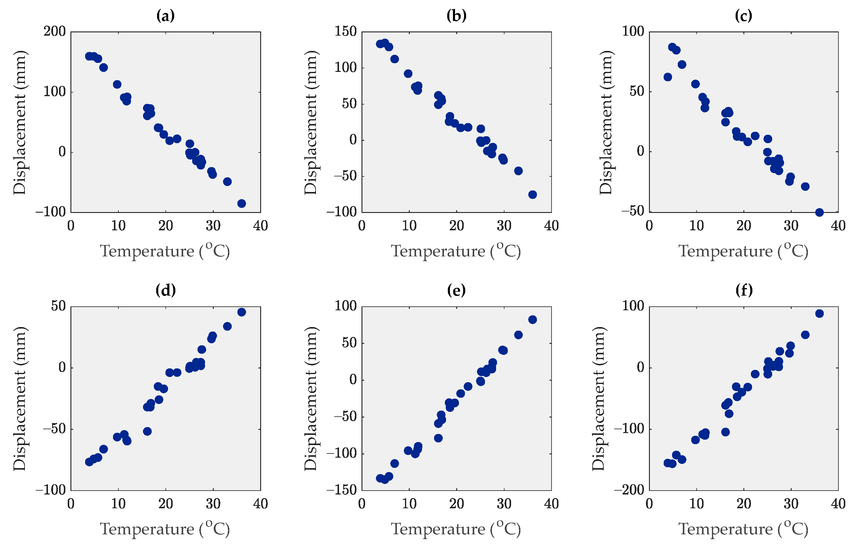
In the problem of the Dashengguan Bridge, where the single measured environmental factor (temperature) and SAR-based displacement data had a strong linear correlation, Kendall’s correlation coefficient could not yield appropriate outputs as good as the MIC, Pearson’s, and Spearman’s correlation coefficient methods. Hence, this correlation measure can be disregarded in further applications.
(3)
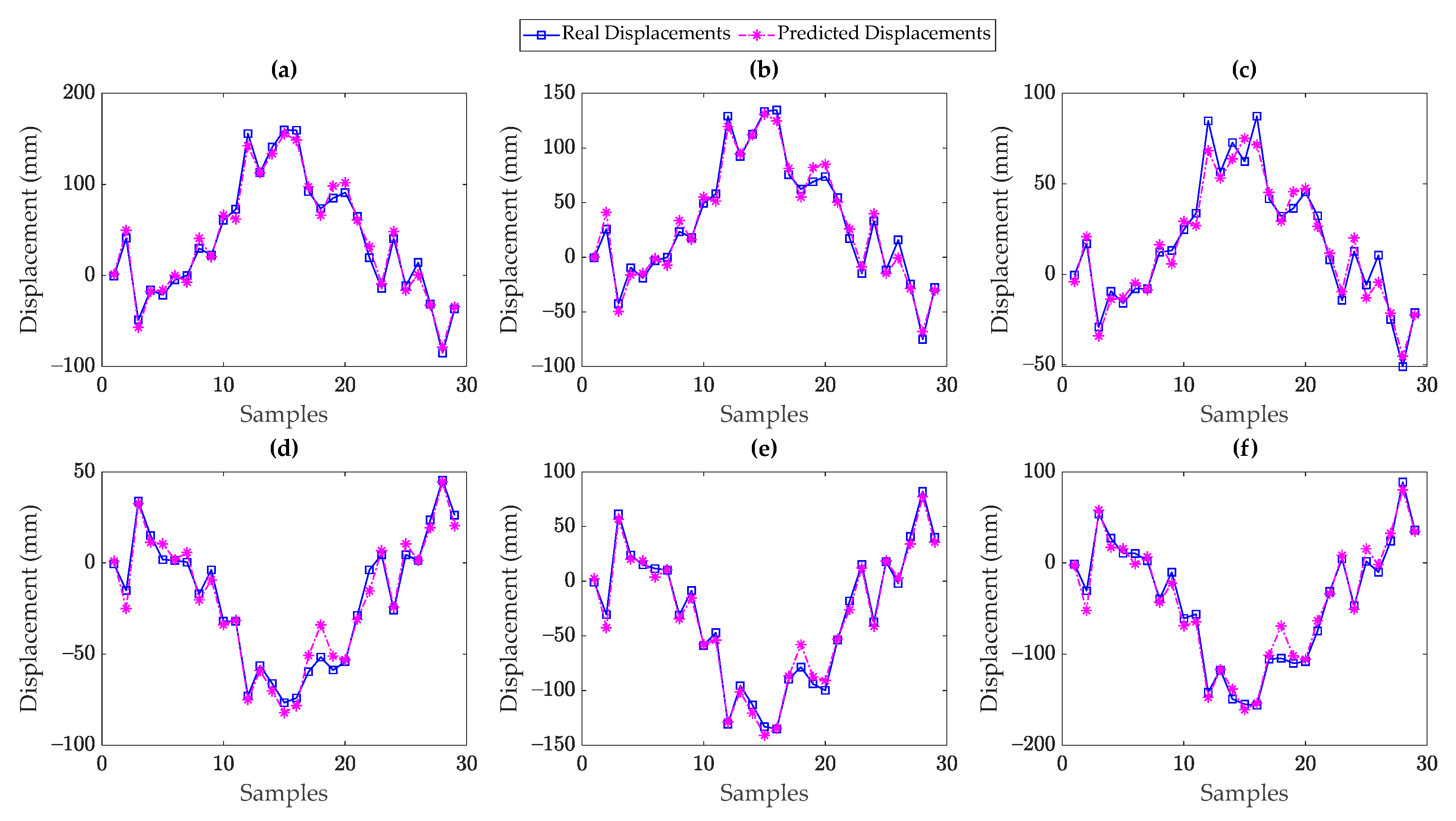
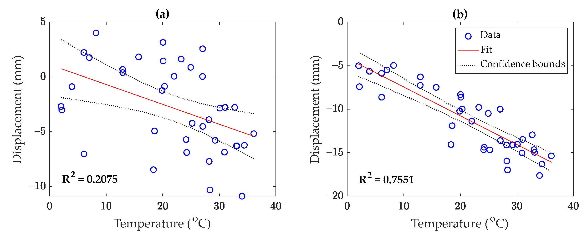
The supervised regression techniques could perform well when there is a high correlation between the displacement and temperature data. These techniques failed in providing accurate and reliable results when the temperature and displacement data had a low correlation. This was most likely due to the fact that the other unmeasured environmental and/or operational conditions or even structural damage impacted the displacement data. Since such conditions were not incorporated into the supervised regression models, those could not properly predict the measured (real) displacement data.
(4)
The low correlation rates and poor prediction performances mean that the environmental/operational sensors (i.e., temperature sensors in this research) in a bridge structure are not sufficient, and one needs to consider further sensors for measuring other environmental and/or operational conditions such as humidity, wind speed and direction, traffic, etc. Moreover, it is important to investigate the possibility of existing any structural damage by visual inspection or tried-and-test techniques for early damage assessment.

Author Contributions

Conceptualization, B.B., A.E. and C.D.M.; methodology, B.B., A.E. and C.D.M.; software, B.B. and A.E.; validation, B.B. and A.E.; formal analysis, B.B., A.E., C.D.M. and A.N.A.; investigation, B.B., A.E., C.D.M. and A.N.A.; resources, B.B. and A.E.; data curation, B.B. and A.E.; writing—original draft preparation, B.B. and A.E.; writing—review and editing, B.B., A.E., C.D.M. and A.N.A.; visualization, B.B., A.E., C.D.M. and A.N.A.; supervision, C.D.M. and A.N.A.; project administration, B.B., A.E., C.D.M. and A.N.A. All authors have read and agreed to the published version of the manuscript.

Funding

This research was partially funded by the European Space Agency (ESA) under ESA contract no. 4000132658/20/NL/MH/ac.

Data Availability Statement

Data is unavailable due to privacy or ethical restrictions.

Conflicts of Interest

The authors declare no conflict of interest.

References

  1. Rizzo, P.; Enshaeian, A. Challenges in Bridge Health Monitoring: A Review. Sensors 2021, 21, 4336. [Google Scholar] [CrossRef] [PubMed]
  2. Chen, Q.; Jiang, W.; Meng, X.; Jiang, P.; Wang, K.; Xie, Y.; Ye, J. Vertical Deformation Monitoring of the Suspension Bridge Tower Using GNSS: A Case Study of the Forth Road Bridge in the UK. Remote Sens. 2018, 10, 364. [Google Scholar] [CrossRef] [Green Version]
  3. Gonen, S.; Erduran, E. A Hybrid Method for Vibration-Based Bridge Damage Detection. Remote Sens. 2022, 14, 6054. [Google Scholar] [CrossRef]
  4. Entezami, A.; Sarmadi, H.; Behkamal, B.; De Michele, C. On continuous health monitoring of bridges under serious environmental variability by an innovative multi-task unsupervised learning method. Struct. Infrastruct. Eng. 2023, in press. [CrossRef]
  5. Daneshvar, M.H.; Sarmadi, H. Unsupervised learning-based damage assessment of full-scale civil structures under long-term and short-term monitoring. Eng. Struct. 2022, 256, 114059. [Google Scholar] [CrossRef]
  6. Gordan, M.; Sabbagh-Yazdi, S.-R.; Ismail, Z.; Ghaedi, K.; Carroll, P.; McCrum, D.; Samali, B. State-of-the-art review on advancements of data mining in structural health monitoring. Measurement 2022, 193, 110939. [Google Scholar] [CrossRef]
  7. Azimi, M.; Eslamlou, A.D.; Pekcan, G. Data-driven structural health monitoring and damage detection through deep learning: State-of-the-art review. Sensors 2020, 20, 2778. [Google Scholar] [CrossRef]
  8. Shen, N.; Chen, L.; Liu, J.; Wang, L.; Tao, T.; Wu, D.; Chen, R. A Review of Global Navigation Satellite System (GNSS)-Based Dynamic Monitoring Technologies for Structural Health Monitoring. Remote Sens. 2019, 11, 1001. [Google Scholar] [CrossRef] [Green Version]
  9. Ferreira, P.M.; Machado, M.A.; Carvalho, M.S.; Vidal, C. Embedded Sensors for Structural Health Monitoring: Methodologies and Applications Review. Sensors 2022, 22, 8320. [Google Scholar] [CrossRef]
  10. Sony, S.; Laventure, S.; Sadhu, A. A literature review of next-generation smart sensing technology in structural health monitoring. Struct. Control Health Monit. 2019, 26, e2321. [Google Scholar] [CrossRef]
  11. Biondi, F.; Addabbo, P.; Ullo, S.L.; Clemente, C.; Orlando, D. Perspectives on the Structural Health Monitoring of Bridges by Synthetic Aperture Radar. Remote Sens. 2020, 12, 3852. [Google Scholar] [CrossRef]
  12. Entezami, A.; Arslan, A.N.; De Michele, C.; Behkamal, B. Online hybrid learning methods for real-time structural health monitoring using remote sensing and small displacement data. Remote Sens. 2022, 14, 3357. [Google Scholar] [CrossRef]
  13. Cigna, F.; Lasaponara, R.; Masini, N.; Milillo, P.; Tapete, D. Persistent Scatterer Interferometry Processing of COSMO-SkyMed StripMap HIMAGE Time Series to Depict Deformation of the Historic Centre of Rome, Italy. Remote Sens. 2014, 6, 12593–12618. [Google Scholar] [CrossRef] [Green Version]
  14. Gama, F.F.; Mura, J.C.; Paradella, W.R.; de Oliveira, C.G. Deformations Prior to the Brumadinho Dam Collapse Revealed by Sentinel-1 InSAR Data Using SBAS and PSI Techniques. Remote Sens. 2020, 12, 3664. [Google Scholar] [CrossRef]
  15. Jänichen, J.; Schmullius, C.; Baade, J.; Last, K.; Bettzieche, V.; Dubois, C. Monitoring of Radial Deformations of a Gravity Dam Using Sentinel-1 Persistent Scatterer Interferometry. Remote Sens. 2022, 14, 1112. [Google Scholar] [CrossRef]
  16. Milillo, P.; Giardina, G.; DeJong, M.J.; Perissin, D.; Milillo, G. Multi-Temporal InSAR Structural Damage Assessment: The London Crossrail Case Study. Remote Sens. 2018, 10, 287. [Google Scholar] [CrossRef] [Green Version]
  17. Milillo, P.; Giardina, G.; Perissin, D.; Milillo, G.; Coletta, A.; Terranova, C. Pre-collapse space geodetic observations of critical infrastructure: The Morandi Bridge, Genoa, Italy. Remote Sens. 2019, 11, 1403. [Google Scholar] [CrossRef] [Green Version]
  18. Pepe, A.; Calò, F. A Review of Interferometric Synthetic Aperture RADAR (InSAR) Multi-Track Approaches for the Retrieval of Earth’s Surface Displacements. Appl. Sci. 2017, 7, 1264. [Google Scholar] [CrossRef] [Green Version]
  19. Deng, Y.; Li, A. Structural Health Monitoring for Suspension Bridges: Interpretation of Field Measurements; Springer: Beijing, China, 2018. [Google Scholar]
  20. Ma, P.; Lin, H.; Wang, W.; Yu, H.; Chen, F.; Jiang, L.; Zhou, L.; Zhang, Z.; Shi, G.; Wang, J. Toward Fine Surveillance: A review of multitemporal interferometric synthetic aperture radar for infrastructure health monitoring. IEEE Geosci. Remote Sens. Mag. 2022, 10, 207–230. [Google Scholar] [CrossRef]
  21. Xia, Y.; Chen, B.; Weng, S.; Ni, Y.-Q.; Xu, Y.-L. Temperature effect on vibration properties of civil structures: A literature review and case studies. J. Civ. Struct. Health Monit. 2012, 2, 29–46. [Google Scholar] [CrossRef] [Green Version]
  22. Han, Q.; Ma, Q.; Xu, J.; Liu, M. Structural health monitoring research under varying temperature condition: A review. J. Civ. Struct. Health Monit. 2020, 11, 149–173. [Google Scholar] [CrossRef]
  23. Farreras-Alcover, I.; Chryssanthopoulos, M.K.; Andersen, J.E. Regression models for structural health monitoring of welded bridge joints based on temperature, traffic and strain measurements. Struct. Health Monit. 2015, 14, 648–662. [Google Scholar] [CrossRef] [Green Version]
  24. Maes, K.; Van Meerbeeck, L.; Reynders, E.P.B.; Lombaert, G. Validation of vibration-based structural health monitoring on retrofitted railway bridge KW51. Mech. Syst. Sig. Process. 2022, 165, 108380. [Google Scholar] [CrossRef]
  25. Laory, I.; Trinh, T.N.; Smith, I.F.C.; Brownjohn, J.M.W. Methodologies for predicting natural frequency variation of a suspension bridge. Eng. Struct. 2014, 80, 211–221. [Google Scholar] [CrossRef] [Green Version]
  26. Wang, Z.; Yang, D.-H.; Yi, T.-H.; Zhang, G.-H.; Han, J.-G. Eliminating environmental and operational effects on structural modal frequency: A comprehensive review. Struct. Control Health Monit. 2022, 29, e3073. [Google Scholar] [CrossRef]
  27. Dervilis, N.; Worden, K.; Cross, E.J. On robust regression analysis as a means of exploring environmental and operational conditions for SHM data. J. Sound Vib. 2015, 347, 279–296. [Google Scholar] [CrossRef] [Green Version]
  28. Roberts, C.; Cava, D.G.; Avendaño-Valencia, L.D. Addressing practicalities in multivariate nonlinear regression for mitigating environmental and operational variations. Struct. Health Monit. 2022, 22, 1237–1255. [Google Scholar] [CrossRef]
  29. Entezami, A.; Mariani, S.; Shariatmadar, H. Damage detection in largely unobserved structures under varying environmental conditions: An autoregressive spectrum and multi-level machine learning methodology. Sensors 2022, 22, 1400. [Google Scholar] [CrossRef]
  30. Sarmadi, H.; Entezami, A.; De Michele, C. Probabilistic data self-clustering based on semi-parametric extreme value theory for structural health monitoring. Mech. Syst. Sig. Process. 2023, 187, 109976. [Google Scholar] [CrossRef]
  31. Daneshvar, M.H.; Sarmadi, H.; Yuen, K.-V. A locally unsupervised hybrid learning method for removing environmental effects under different measurement periods. Measurement 2023, 208, 112465. [Google Scholar] [CrossRef]
  32. Entezami, A.; Sarmadi, H.; Behkamal, B. Long-term health monitoring of concrete and steel bridges under large and missing data by unsupervised meta learning. Eng. Struct. 2023, 279, 115616. [Google Scholar] [CrossRef]
  33. Sarmadi, H.; Entezami, A.; Magalhães, F. Unsupervised data normalization for continuous dynamic monitoring by an innovative hybrid feature weighting-selection algorithm and natural nearest neighbor searching. Struct. Health Monit. 2023, in press. [CrossRef]
  34. Sarmadi, H.; Yuen, K.-V. Structural health monitoring by a novel probabilistic machine learning method based on extreme value theory and mixture quantile modeling. Mech. Syst. Sig. Process. 2022, 173, 109049. [Google Scholar] [CrossRef]
  35. Xu, X.; Huang, Q.; Ren, Y.; Zhao, D.-Y.; Yang, J.; Zhang, D.-Y. Modeling and Separation of Thermal Effects from Cable-Stayed Bridge Response. J. Bridge Eng. 2019, 24, 04019028. [Google Scholar] [CrossRef]
  36. Teng, J.; Tang, D.-H.; Hu, W.-H.; Lu, W.; Feng, Z.-W.; Ao, C.-F.; Liao, M.-H. Mechanism of the effect of temperature on frequency based on long-term monitoring of an arch bridge. Struct. Health Monit. 2021, 20, 1716–1737. [Google Scholar] [CrossRef]
  37. Murphy, B.; Yarnold, M. Temperature-driven structural identification of a steel girder bridge with an integral abutment. Eng. Struct. 2018, 155, 209–221. [Google Scholar] [CrossRef]
  38. Zhou, Y.; Sun, L. Effects of environmental and operational actions on the modal frequency variations of a sea-crossing bridge: A periodicity perspective. Mech. Syst. Sig. Process. 2019, 131, 505–523. [Google Scholar] [CrossRef]
  39. Mao, J.-X.; Wang, H.; Feng, D.-M.; Tao, T.-Y.; Zheng, W.-Z. Investigation of dynamic properties of long-span cable-stayed bridges based on one-year monitoring data under normal operating condition. Struct. Control Health Monit. 2018, 25, e2146. [Google Scholar] [CrossRef]
  40. Yang, D.-H.; Yi, T.-H.; Li, H.-N.; Zhang, Y.-F. Monitoring and analysis of thermal effect on tower displacement in cable-stayed bridge. Measurement 2018, 115, 249–257. [Google Scholar] [CrossRef]
  41. Xia, Q.; Zhang, J.; Tian, Y.; Zhang, Y. Experimental Study of Thermal Effects on a Long-Span Suspension Bridge. J. Bridge Eng. 2017, 22, 04017034. [Google Scholar] [CrossRef]
  42. Moser, P.; Moaveni, B. Environmental effects on the identified natural frequencies of the Dowling Hall Footbridge. Mech. Syst. Sig. Process. 2011, 25, 2336–2357. [Google Scholar] [CrossRef]
  43. Hu, W.H.; Cunha, Á.; Caetano, E.; Rohrmann, R.; Said, S.; Teng, J. Comparison of different statistical approaches for removing environmental/operational effects for massive data continuously collected from footbridges. Struct. Control Health Monit. 2016, 24, e1955. [Google Scholar] [CrossRef]
  44. Qin, Y.; Li, Y.; Liu, G. Separation of the Temperature Effect on Structure Responses via LSTM-Particle Filter Method Considering Outlier from Remote Cloud Platforms. Remote Sens. 2022, 14, 4629. [Google Scholar] [CrossRef]
  45. Jang, J.; Smyth, A.W. Data-driven models for temperature distribution effects on natural frequencies and thermal prestress modeling. Struct. Control Health Monit. 2020, 27, e2489. [Google Scholar] [CrossRef]
  46. Huang, Q.; Crosetto, M.; Monserrat, O.; Crippa, B. Displacement monitoring and modelling of a high-speed railway bridge using C-band Sentinel-1 data. ISPRS J. Photogramm. Remote Sens. 2017, 128, 204–211. [Google Scholar] [CrossRef]
  47. Qin, X.; Zhang, L.; Yang, M.; Luo, H.; Liao, M.; Ding, X. Mapping surface deformation and thermal dilation of arch bridges by structure-driven multi-temporal DInSAR analysis. Remote Sens. Environ. 2018, 216, 71–90. [Google Scholar] [CrossRef]
  48. Li, S.; Li, H.; Liu, Y.; Lan, C.; Zhou, W.; Ou, J. SMC structural health monitoring benchmark problem using monitored data from an actual cable-stayed bridge. Struct. Control Health Monit. 2014, 21, 156–172. [Google Scholar] [CrossRef]
  49. Ding, Y.; Ye, X.W.; Guo, Y. Data set from wind, temperature, humidity and cable acceleration monitoring of the Jiashao bridge. J. Civ. Struct. Health Monit. 2023, 13, 579–589. [Google Scholar] [CrossRef]
  50. Fenerci, A.; Kvåle, K.A.; Petersen, Ø.W.; Rønnquist, A.; Øiseth, O. Data Set from Long-Term Wind and Acceleration Monitoring of the Hardanger Bridge. J. Struct. Eng. 2021, 147, 04721003. [Google Scholar] [CrossRef]
  51. Niu, Y.; Ye, Y.; Zhao, W.; Duan, Y.; Shu, J. Identifying Modal Parameters of a Multispan Bridge Based on High-Rate GNSS-RTK Measurement Using the CEEMD-RDT Approach. J. Bridge Eng. 2021, 26, 04021049. [Google Scholar] [CrossRef]
  52. Salvadori, G.; De Michele, C.; Kottegoda, N.T.; Rosso, R. Extremes in Nature: An Approach Using Copulas; Springer: Berlin/Heidelberg, Germany, 2007. [Google Scholar]
  53. Reshef, D.N.; Reshef, Y.A.; Finucane, H.K.; Grossman, S.R.; McVean, G.; Turnbaugh, P.J.; Lander, E.S.; Mitzenmacher, M.; Sabeti, P.C. Detecting novel associations in large data sets. Science 2011, 334, 1518–1524. [Google Scholar] [CrossRef] [PubMed] [Green Version]
  54. Schulz, E.; Speekenbrink, M.; Krause, A. A tutorial on Gaussian process regression: Modelling, exploring, and exploiting functions. J. Math. Psychol. 2018, 85, 1–16. [Google Scholar] [CrossRef]
  55. Rasmussen, C.E.; Williams, C.K.I. Gaussian Processes for Machine Learning; MIT Press: Cambridge, MA, USA, 2005. [Google Scholar]
  56. Pisner, D.A.; Schnyer, D.M. Support vector machine. In Machine Learning; Mechelli, A., Vieira, S., Eds.; Academic Press: Cambridge, MA, USA, 2020; pp. 101–121. [Google Scholar] [CrossRef]
  57. Smola, A.J.; Schölkopf, B. A tutorial on support vector regression. Stat. Comput. 2004, 14, 199–222. [Google Scholar] [CrossRef] [Green Version]
Figure 1. (a) The Dashengguan Bridge, (b) the side view and main dimensions.
Remotesensing 15 03503 g001
Figure 2. The Dashengguan Bridge: (a) limited displacement data from remote sensing, (b) temperature data from contact sensing.
Remotesensing 15 03503 g002
Figure 3. (a) The Lupu Bridge, (b) the side view and main dimensions.
Remotesensing 15 03503 g003
Figure 4. The limited displacements of the Lupu Bridge from 38 SAR images of TerraSAR-X between 2013–2016: (a) the dome, (b) the main span, (c) the temperature data.
Remotesensing 15 03503 g004
Figure 5. (a) The Rainbow Bridge, (b) the side view and main dimensions.
Remotesensing 15 03503 g005
Figure 6. The limited displacements of the Lupu Bridge from 53 SAR images of Sentinel-1A between 2015–2017: (a) Piers #1–4, (b) Spans #1–3, (c) temperature data.
Remotesensing 15 03503 g006
Figure 7. Scatter plots of the displacement versus temperature data in the problem of the Dashengguan Bridge: (a) Pier #4, (b) Pier #5, (c) Pier #6, (d) Pier #8, (e) Pier #9, (f) Pier #10.
Remotesensing 15 03503 g007
Figure 8. LRMs fitted to the displacement and temperature data of the Dashengguan Bridge: (a) Pier 4, (b) Pier 5, (c) Pier 6, (d) Pier 8, (e) Pier 9, (f) Pier 10.
Remotesensing 15 03503 g008
Figure 9. Bayesian hyperparameter optimization of the kernel parameters of κ S related to the GPR models of Piers 4–6 and 8–10 of the Dashengguan Bridge: (a) σS, (b) λS.
Remotesensing 15 03503 g009
Figure 10. Bayesian hyperparameter optimization of the SVR models related to Piers 4–6 and 8–10 of the Dashengguan Bridge: (a) the number of support vectors, (b) the model bias values.
Remotesensing 15 03503 g010
Figure 11. Real and predicted displacement data of the Dashengguan Bridge based on the LRMs: (a) Pier 4, (b) Pier 5, (c) Pier 6, (d) Pier 8, (e) Pier 9, (f) Pier 10.
Remotesensing 15 03503 g011
Figure 12. Real and predicted displacement data of the Dashengguan Bridge based on the GPR models: (a) Pier 4, (b) Pier 5, (c) Pier 6, (d) Pier 8, (e) Pier 9, (f) Pier 10.
Remotesensing 15 03503 g012
Figure 13. Real and predicted displacement data of the Dashengguan Bridge based on the SVR models: (a) Pier 4, (b) Pier 5, (c) Pier 6, (d) Pier 8, (e) Pier 9, (f) Pier 10.
Remotesensing 15 03503 g013
Figure 14. Scatter plots of the displacement and temperature data of the Lupu Bridge: (a) the dome, (b) the main span.
Remotesensing 15 03503 g014
Figure 15. LRMs fitted to the displacement and temperature data of the Lupu Bridge: (a) the dome, (b) the main span.
Remotesensing 15 03503 g015
Figure 16. Real and predicted displacement data of the Lupu Bridge based on the LRMs: (a) the dome, (b) the main span.
Remotesensing 15 03503 g016
Figure 17. Real and predicted displacement data of the Lupu Bridge based on the GPR models: (a) the dome, (b) the main span.
Remotesensing 15 03503 g017
Figure 18. Real and predicted displacement data of the Lupu Bridge based on the SVR models: (a) the dome, (b) the main span.
Remotesensing 15 03503 g018
Figure 19. Scatter plots of the displacement and temperature data of the Rainbow Bridge: (a) Pier 1, (b) Pier 2, (c) Pier 3, (d) Pier 4.
Remotesensing 15 03503 g019
Figure 20. Scatter plots of the displacement and temperature data of the Rainbow Bridge: (a) Span 1, (b) Span 2, (c) Span 3.
Remotesensing 15 03503 g020
Figure 21. LRMs fitted to the displacement and temperature data of the Rainbow Bridge: (a) Pier 1, (b) Pier 2, (c) Pier 3, (d) Pier 4.
Remotesensing 15 03503 g021
Figure 22. LRMs fitted to the displacement and temperature data of the Rainbow Bridge: (a) Span 1, (b) Span 2, (c) Span 3.
Remotesensing 15 03503 g022
Figure 23. Real and predicted displacement data of the Rainbow Bridge based on the LRMs: (a) Pier 1, (b) Pier 2, (c) Pier 3, (d) Pier 4.
Remotesensing 15 03503 g023
Figure 24. Real and predicted displacement data of the Rainbow Bridge based on the LRMs: (a) Span 1, (b) Span 2, (c) Span 3.
Remotesensing 15 03503 g024
Figure 25. Bayesian hyperparameter optimization of the kernel parameters of κ S related to the GPR models of Piers 1–4 and Spans 1–3 of the Rainbow Bridge: (a) σS, (b) λS.
Remotesensing 15 03503 g025
Figure 26. Bayesian hyperparameter optimization of the SVR models related to Piers 1–4 and Spans 1–3 of the Rainbow Bridge: (a) the number of support vectors, (b) the model bias values.
Remotesensing 15 03503 g026
Figure 27. Real and predicted displacement data of the Rainbow Bridge based on the GPR models: (a) Pier 1, (b) Pier 2, (c) Pier 3, (d) Pier 4.
Remotesensing 15 03503 g027
Figure 28. Real and predicted displacement data of the Rainbow Bridge based on the GPR models: (a) Span 1, (b) Span 2, (c) Span 3.
Remotesensing 15 03503 g028
Figure 29. Real and predicted displacement data of the Rainbow Bridge based on the SVR models: (a) Pier 1, (b) Pier 2, (c) Pier 3, (d) Pier 4.
Remotesensing 15 03503 g029
Figure 30. Real and predicted displacement data of the Rainbow Bridge based on the SVR models: (a) Span 1, (b) Span 2, (c) Span 3.
Remotesensing 15 03503 g030
Table 1. Correlation analysis between limited displacement and temperature data regarding the Dashengguan Bridge.
Pier No.MICCorrelation Coefficient Metrics
PearsonSpearmanKendall
41.00−0.9928−0.9931−0.9507
51.00−0.9899−0.9896−0.9310
61.00−0.9776−0.9822−0.9064
81.000.98500.99010.9359
91.000.99430.99400.9507
101.000.98770.98760.9211
Table 2. Correlation analysis between limited displacement and temperature data regarding the Lupu Bridge.
ComponentCorrelation Coefficient Metrics
MICPearsonSpearmanKendall
Dome0.56−0.4555−0.4925−0.3285
Span0.90−0.8689−0.8483−0.6557
Table 3. Correlation analysis between the limited displacement data related to the piers and spans of the Rainbow Bridge and temperature records.
ElementsMICCorrelation Coefficient Metrics
PearsonSpearmanKendall
Pier 10.720.60810.62890.4296
Pier 20.610.41940.41510.2946
Pier 30.330.25210.24390.1625
Pier 40.390.37450.36120.2481
Span 10.75−0.7140−0.7184−0.5326
Span 20.70−0.6793−0.7005−0.5195
Span 30.74−0.7165−0.7281−0.5442
Table 4. The decision on the sufficiency of temperature sensors for structural response evaluation.
Bridge NameElementsCorrelation RatePrediction AccuracyDecision
LinearNonlinear
DashengguanPiers 4–6 & 8–10HighHighHighSufficient
LupuDomeLowLowLowInsufficient
SpanHighHighHighSufficient
RainbowPier 1LowLowLowInsufficient
Pier 2LowLowHigh *Sufficient *
Pier 3LowLowHigh *Sufficient *
Pier 4LowLowLowInsufficient
Span 1HighHighLowInsufficient **
Span 2HighHighLowInsufficient **
Span 3HighHighLowInsufficient **
Note: The expressions “High *” and “Sufficient *” are based on the prediction via the GPR. Moreover, the term “Insufficient **” refers to the possibility of the existence of structural damage. The green color refers to the high correlation rate, high prediction accuracy, and sufficient sensor numbers. The red color refers to the low correlation rate, low prediction accuracy, and insufficient sensor numbers.
Disclaimer/Publisher’s Note: The statements, opinions and data contained in all publications are solely those of the individual author(s) and contributor(s) and not of MDPI and/or the editor(s). MDPI and/or the editor(s) disclaim responsibility for any injury to people or property resulting from any ideas, methods, instructions or products referred to in the content.

