Article

A Novel Framework for Stratified-Coupled BLS Tree Trunk Detection and DBH Estimation in Forests (BSTDF) Using Deep Learning and Optimization Adaptive Algorithm

1
Institute of Forest Resource Information Techniques, Chinese Academy of Forestry, Beijing 100091, China
2
Experimental Center of Subtropical Forestry, Chinese Academy of Forestry, Fenyi 336600, China
3
Key Laboratory of Forestry Remote Sensing and Information System, NFGA, Beijing 100091, China
*
Author to whom correspondence should be addressed.
Remote Sens. 2023, 15(14), 3480; https://doi.org/10.3390/rs15143480
Submission received: 20 April 2023 / Revised: 30 June 2023 / Accepted: 7 July 2023 / Published: 10 July 2023

Abstract

:
Diameter at breast height (DBH) is a critical metric for quantifying forest resources, and obtaining accurate, efficient measurements of DBH is crucial for effective forest management and inventory. A backpack LiDAR system (BLS) can provide high-resolution representations of forest trunk structures, making it a promising tool for DBH measurement. However, in practical applications, deep learning-based tree trunk detection and DBH estimation using BLS still faces numerous challenges, such as complex forest BLS data, low proportions of target point clouds leading to imbalanced class segmentation accuracy in deep learning models, and low fitting accuracy and robustness of trunk point cloud DBH methods. To address these issues, this study proposed a novel framework for BLS stratified-coupled tree trunk detection and DBH estimation in forests (BSTDF). This framework employed a stratified coupling approach to create a tree trunk detection deep learning dataset, introduced a weighted cross-entropy focal-loss function module (WCF) and a cosine annealing cyclic learning strategy (CACL) to enhance the WCF-CACL-RandLA-Net model for extracting trunk point clouds, and applied a (least squares adaptive random sample consensus) LSA-RANSAC cylindrical fitting method for DBH estimation. The findings reveal that the dataset based on the stratified-coupled approach effectively reduces the amount of data for deep learning tree trunk detection. To compare the accuracy of BSTDF, synchronous control experiments were conducted using the RandLA-Net model and the RANSAC algorithm. To benchmark the accuracy of BSTDF, we conducted synchronized control experiments utilizing a variety of mainstream tree trunk detection models and DBH fitting methodologies. Especially when juxtaposed with the RandLA-Net model, the WCF-CACL-RandLA-Net model employed by BSTDF demonstrated a 6% increase in trunk segmentation accuracy and a 3% improvement in the F1 score with the same training sample volume. This effectively mitigated class imbalance issues encountered during the segmentation process. Simultaneously, when compared to RANSAC, the LSA-RANCAC method adopted by BSTDF reduced the RMSE by 1.08 cm and boosted R2 by 14%, effectively tackling the inadequacies of RANSAC’s filling. The optimal acquisition distance for BLS data is 20 m, at which BSTDF’s overall tree trunk detection rate (ER) reaches 90.03%, with DBH estimation precision indicating an RMSE of 4.41 cm and R2 of 0.87. This study demonstrated the effectiveness of BSTDF in forest DBH estimation, offering a more efficient solution for forest resource monitoring and quantification, and possessing immense potential to replace field forest measurements.

1. Introduction

Diameter at breast height (DBH, 1.30 m high) is one of the key indices for forest inventory, reflecting forest growth conditions and carbon storage distribution, and constituting an essential component of foundational forestry data [1]. Light detection and ranging (LiDAR), an active remote sensing technology, can provide high-resolution descriptions of forest trunk structures and possesses significant advantages in DBH estimation [1,2,3,4,5,6]. Currently, LiDAR systems mainly include terrestrial laser scanners (TLS), airborne laser scanners (ALS), and mobile laser scanners (MLS). High-density point cloud data acquired by TLS enables the measurement of millimeter-precision 3D tree structures, such as tree height, DBH, and crown diameter [7]. However, in practical applications, single-site TLS scanning exhibits a relatively high trunk non-detection rate (17.4–32%) [8,9], while multi-site scanning necessitates higher processing costs and is unsuitable for large-scale forest parameter acquisition. ALS can rapidly obtain extensive forest point clouds, but in dense stands, the light beams are often obstructed by tree crowns [4], which hinders tree trunk detection and DBH estimation. MLS systems offer powerful tools for addressing tree occlusion and immobility issues, effectively reducing time and labor costs [10]. However, the accuracy of MLS data is typically lower than that of multi-site TLS data [8], and the application conditions of MLS are susceptible to the GNSS signal, terrain, and other objective environmental factors [9]. With the rapid reduction in size and weight of laser scanners and the development of GNSS technology, the emergence of Backpack LiDAR systems (BLS) has compensated for the limitations of other LiDAR technologies. As a backpack-style form of MLS, BLS collects data by walking and exhibits higher scanning efficiency [5], making it highly suitable for large-scale forest tree trunk detection and DBH information extraction.
At present, there are numerous methods for estimating DBH based on LiDAR, including least squares (geometric) circle fitting (LS) [11,12], cylindrical fitting (CF) [13], Hough transform (HT) [14], convex hull algorithm (CHA) [11], and random sample consensus (RANSAC) [3]. These methods are prone to interference from factors such as noise and foliage occlusion during the fitting process, which can lead to reduced fitting accuracy. Consequently, optimizing the fitting methods to enhance accuracy and robustness is crucial. In the DBH fitting process, typical steps include “ground point identification—trunk localization—point cloud slicing at DBH—DBH estimation” [2,8,10,15,16,17]. In this process, separating trunk point cloud data from non-trunk point cloud data is one of the key steps that aim to eliminate noise interference and prevent the misestimation of DBH. However, achieving accurate and efficient tree trunk detection in forest BLS data still presents challenges. Visual interpretation is the most accurate method for eliminating non-trunk point clouds, yet this approach requires skilled professionals and is more labor-intensive. Utilizing a computer to extract the linear spatial features of tree trunk point clouds for cylindrical detection has proven efficient [18,19], yet its precision diminishes in the face of complex forest spatial structures. As such, the development of a tree trunk detection framework or method adaptable to forest scenarios has become pressing. After all, tree trunk detection lays the groundwork for calculating forest resources, such as DBH [20], volume estimation, and individual tree segmentation [21].
Computers based on deep learning technology possess strong memory and learning capabilities [16,20,21,22,23], effectively addressing the limitations of traditional DBH estimation methods in extracting forest DBH information, such as their difficulty in point cloud noise recognition, insufficient robustness, and low extraction efficiency. By learning trunk features, repeatable and scalable trunk recognition and localization tasks with large amounts of data can be achieved. Currently, mainstream deep learning methods such as PointNet [23,24], KPConv [25], DCNN [26], and PointCNN [27] have been applied to point cloud segmentation. Most of these methods use the farthest point sampling (FPS) to retain point cloud spatial features as much as possible, but the processing speed is slow for larger datasets (1.0 × 10⁵ and above). In summary, for tree trunk detection and DBH estimation in complex forests, researchers can improve processing capabilities and extraction accuracy by focusing on dataset creation, deep learning models, and DBH fitting algorithms.
In a bid to overcome the challenges mentioned earlier, we put forth a novel framework for deep learning-based tree trunk detection and diameter at breast height (DBH) estimation, leveraging BLS hierarchical coupling (BSTDF). This innovation facilitated effective tree trunk identification and DBH estimation from MLS point cloud data. Furthermore, we delved into the impact of varying MLS scanning distance levels on the precision of tree trunk detection and DBH estimation. The main contributions of the proposed framework are as follows:
(1)
In light of the substantial volume of point cloud data in forest scenarios, we introduced a novel approach to constructing a deep learning tree trunk detection dataset, which is predicated on hierarchical coupling. This approach effectively curtails the data volume necessary during the tree trunk detection process;
(2)
To rectify the issue of uneven class accuracy in point cloud segmentation within the RandLA-Net model for tree trunk detection scenarios, we introduced an enhanced RandLA-Net semantic segmentation model with dual modules (WCF and CACL). By increasing the model’s attention towards the target classes and employing more flexible learning strategies, we improved the segmentation accuracy for the tree trunk class, ultimately leading to an elevated detection rate;
(3)
We enhanced the RANCAC algorithm by implementing an adaptive approach and a least squares optimization algorithm. These meticulously devised strategies served to optimize the fitting model parameters and boost the convergence of model error, thereby significantly elevating the accuracy of the DBH fitting within forest scenarios;
(4)
Lastly, having conducted a comparative analysis of the precision of tree trunk detection and DBH fitting at different MLS scanning distance levels, we proposed a recommended distance for MLS scanning, which offers a balance between data quality and scanning efficiency.

2. Materials and Methods

2.1. Study Area

The study area for this paper encompasses a series of forest stands on both sides of the main road in the Tree Garden of the Subtropical Forestry Experiment Center, part of the Chinese Academy of Forestry. The study area has an average slope of 5°, with higher elevation in the south and lower elevation in the north. Covering a total area of 65,000 m2 (650 m × 100 m) and extending in a north–south direction, it is located in the northwestern part of Fenyi County, Jiangxi Province (Figure 1A,B). With abundant forest resources, Fenyi County has a forest coverage rate of 65.76%. The main tree species in the area include Chinese fir, Masson pine, Schima superba, camphor, and Machilus thunbergii, which are typical tree species in southern China. The regional vegetation is characterized by mid-subtropical evergreen broad-leaved forests, with a frost-free period of 240–307 days. The annual average rainfall ranges from 1500 to 1700 mm, while the annual average temperature lies between 11.6 and 19.3 °C. The lowest temperature in January is 3.2 to 4.7 °C, and the highest temperature in July is 29.8 to 38.3 °C.

2.2. Data

2.2.1. Field Survey Data

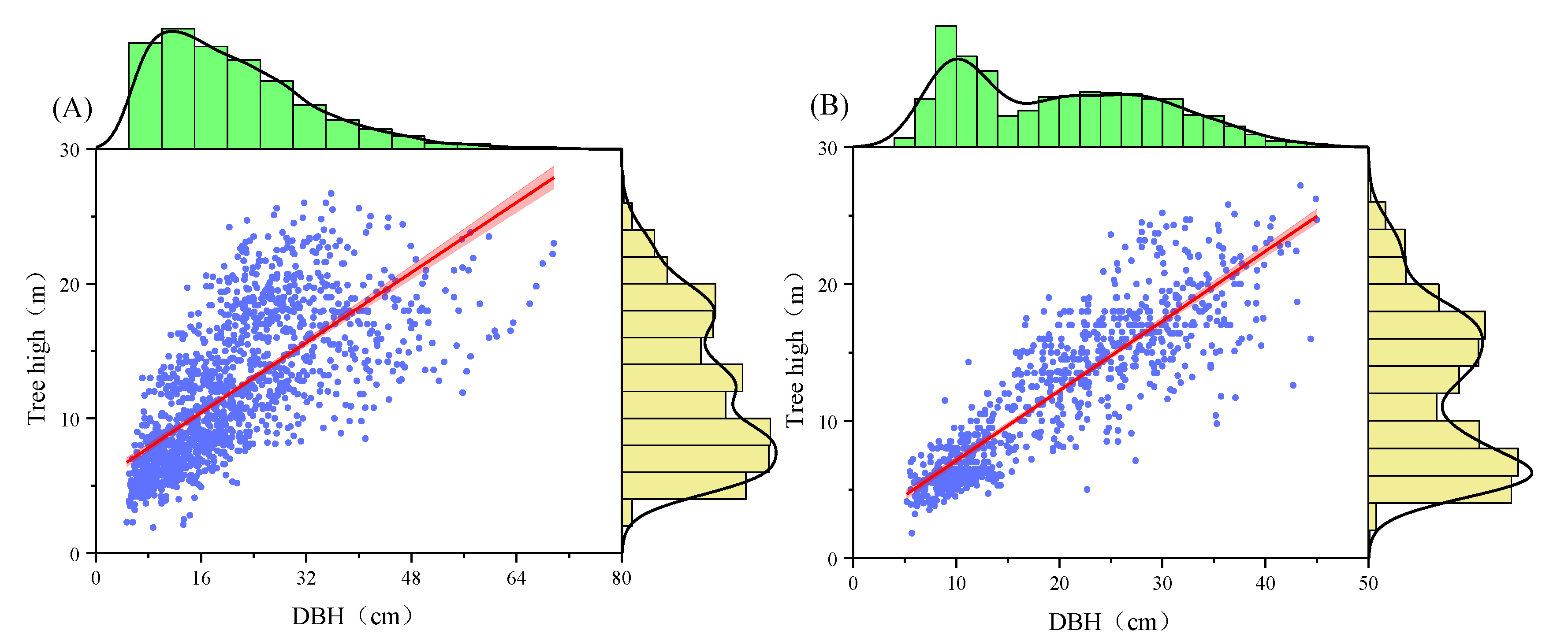
Field surveys were undertaken in April and May of 2022. A comprehensive inventory was completed on a tree-by-tree basis within the study area, using the Real-Time Kinematic Global Navigation Satellite System (RTK-GNSS) to determine the location of each sample tree. Our inventory criteria were set for trees with a diameter at breast height (DBH) greater than 5 cm, and we measured and recorded tree height, DBH, crown width, tree species, and location information. Both the DBH and crown width were gauged using a tape measure, while tree height was measured with a laser rangefinder and various environmental factors of the plot were recorded. Figure 1C illustrates the spatial distribution characteristics of trees within the study area. Table 1 presents the statistical features of trees in the study area. Figure 2A displays the scatter distribution of broadleaf tree DBH and trunk fitting within the study area, while Figure 2B exhibits the scatter distribution of conifer tree DBH and trunk fitting within the study area. The data revealed that there were 2303 trees in the study area, comprising 47 broad-leaved species and 15 coniferous species. The principal broad-leaved species included Michelia, camphor, birch, Eucalyptus, and osmanthus, while the main coniferous species consisted of cypress, Cryptomeria, Taxodium, and Thuja. The average DBH values of various tree species ranged from 9.08 cm to 32.77 cm. In this paper, field measurement results will serve as validation data for the experimental results.
Dividing the dataset is a foundational step in training deep learning models. In our research, we categorized the trees surveyed within the entire research area into training, validation, and testing zones based on their functional regions.
Within the training zone, there were a total of 453 trees, with an average DBH of 21.34 cm and an average standard deviation of DBH at 9.83 cm. The validation zone comprised 220 trees, with an average DBH of 19.24 cm and an average standard deviation of DBH of 9.52 cm. The testing zone included 1851 trees, with an average DBH of 20.78 cm and an average standard deviation of DBH of 11.20 cm. The types of trees and the diameter distribution across all three functional zones were relatively balanced, providing representative samples. Table 1 displays the data features of the trees in each functional zone within the research area.

2.2.2. BLS Data

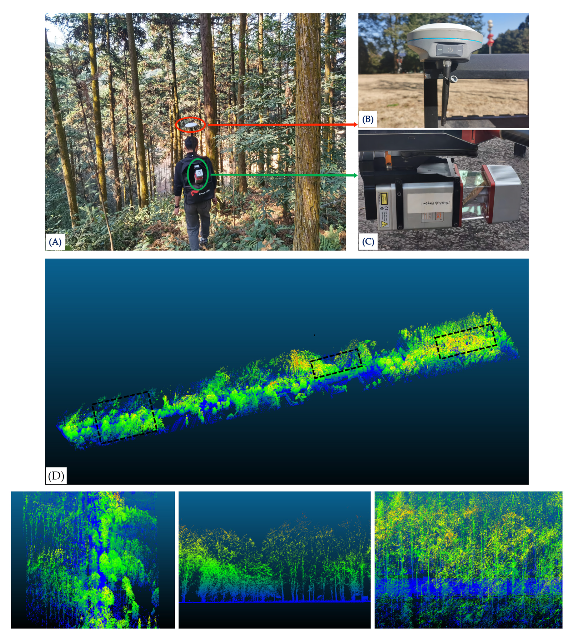
The BLS used in this study was the RIEGL miniVUX 1UAV (Figure 3C), equipped with the RIEGL miniVUX 3D laser scanner and Trimble APX-15 GNSS Inertial Navigation OEM (Figure 3B). The measurement trajectory of the BLS is shown in Figure 1C. The scanner system was initialized within the plot, and the plot was covered by a single pass of a rectangular transect. The BLS system’s positioning relies on SLAM systems, GNSS positioning, and an inertial measurement unit. During the data collection process, the operator walked at a speed of 5 km/h, generating a high-density BLS data point cloud of approximately 600 points/m2.

2.3. Methods

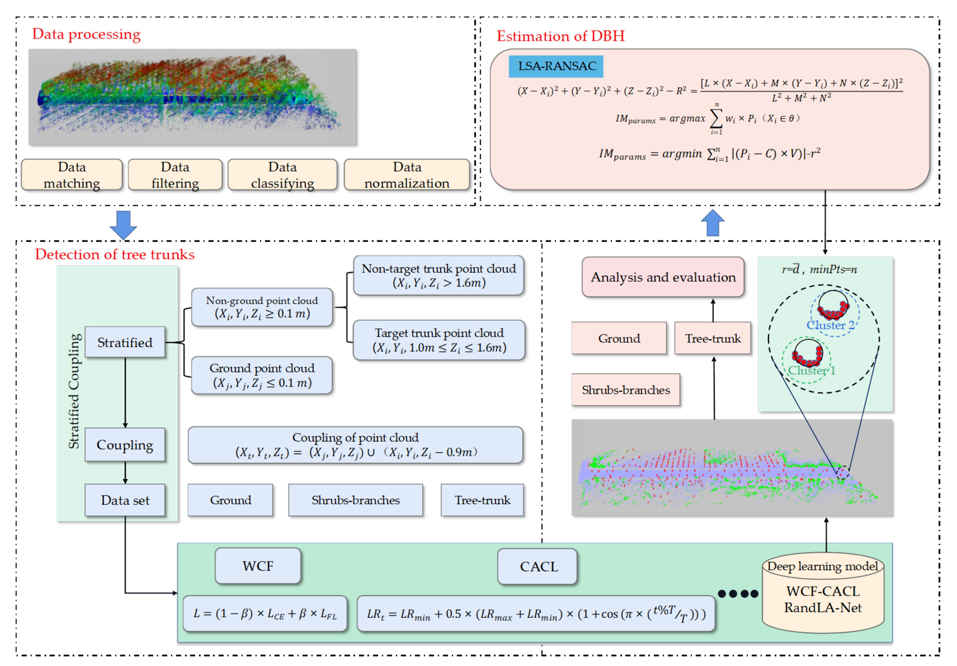
In this study, we created a stratified coupled tree trunk detection deep learning dataset based on BLS data and improved the WCF-CACL-RandLA-Net model and LSA-RANSAC algorithm to achieve tree trunk detection (Objective 1) and DBH estimation (Objective 2) within the study area. The flowchart of this study is shown in Figure 4.

2.3.1. Creation of the Tree Trunk Detection Deep Learning Dataset Based on Stratified Coupling

Using BLS as the base data and referencing the basic requirements of the RandLA-Net model for the dataset, we applied a novel stratified coupling method to create the tree trunk detection deep learning dataset to reduce data volume and enhance model learning efficiency. Through this method, we reduced the point cloud count from the original forest point cloud of 1.43 × 10⁸ to the stratified coupling dataset of 6.14 × 10⁶.
Step 1: BLS data preprocessing. We set the initial data input as ( X i , Y i , Z i ). However, we noted that the point cloud contained many noise points, which were filtered out using a density-based criterion. The filtered point cloud data were classified into a ground point cloud and a vegetation point cloud. Finally, we normalized the vegetation point cloud using a high-precision DEM model.
Step 2: Stratification of the normalized point cloud. We stratified the normalized point cloud into three categories, including a ground point cloud layer ( X j ,   Y j ,   Z j ), a target point cloud layer ( X t , Y t , Z t ), and a non-target point cloud layer ( X n , Y n , Z n ).
( X j , Y j , Z j ) = ( X i , Y i , Z i < 0.1   m )
( X t , Y t , z t ) = ( X i , Y i , 1.0   m Z i 1.6   m )
( X n , Y n , Z n ) = ( X i , Y i , Z i < 1.0   m     Z i > 1.6   m )
Step 3: Coupling of the stratified point clouds. To ensure the spatial structural continuity of the stratified point clouds and improve the deep learning model’s training efficiency, we coupled the stratified point clouds. The coupled point cloud output was set as (X, Y, Z).
( X t , Y t , Z t ) = ( X j , Y j , Z j )   ( X t , Y t , Z t 0.9   m )
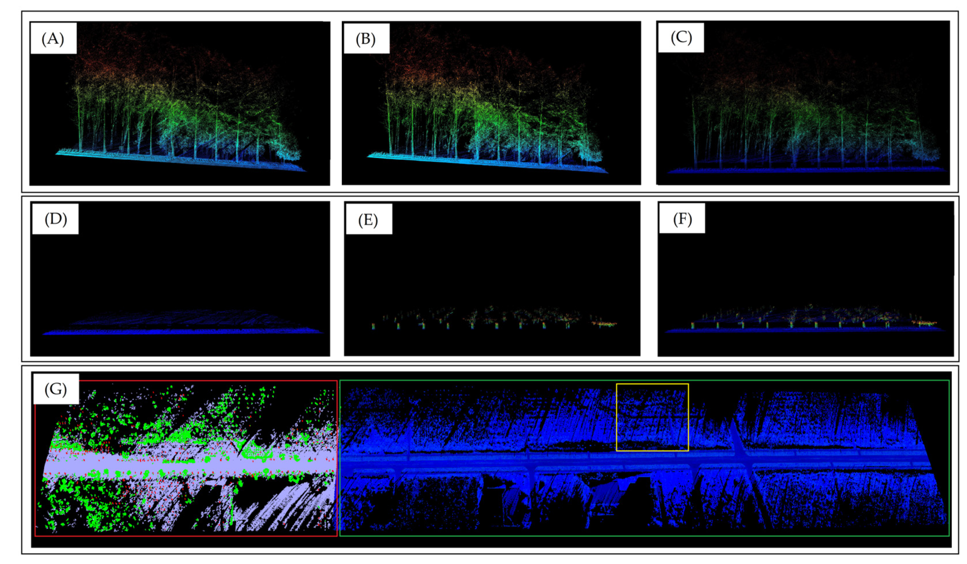
Step 4: Dataset partitioning. The total number of BLS point clouds after stratified coupling was 6.14 × 10⁶, divided into the training dataset (TDS), validation dataset (VDS), and partition dataset (PDS), with quantities of 2.12 × 10⁶, 1.02 × 10⁴, and 4.01 × 10⁶, respectively. In the training and validation data, we manually annotated three types using CloudCompare 2.11.3, including (1) tree trunk point clouds (Tree-trunk), (2) shrub and tree branch point clouds (Shrubs-branches), and (3) ground and understory vegetation point clouds (Ground). Statistics show that in TDS, the number of Tree-trunk, Shrubs-branches, and Ground were 6.08 × 10⁴, 1.53 × 10⁵, and 1.90 × 10⁶, respectively. In the VDS, the numbers were 0.95 × 10⁴, 1.74 × 10⁴, and 7.23 × 10⁴, respectively. Figure 5 displays the dataset creation process and Figure 5G shows the spatial distribution of TDS, VDS, and PDS dataset partitioning.
Step 5: Data augmentation. Point cloud data augmentation refers to the transformation and processing of the original point cloud data to increase the training samples, enhancing the model’s generalization capability and accuracy. Data augmentation helps to address issues such as data scarcity, uneven sample distribution, and overfitting. In this study, we enhanced training samples using rotation and scaling, where rotation was performed clockwise around the X, Y, and Z axes by 180°, and the scaling factor was set to 0.8 and 1.2. After data augmentation, the training samples were expanded by 6 times to 1.27 × 10⁷.

2.3.2. Construction of the WCF-CACL-RandLA-Net Model

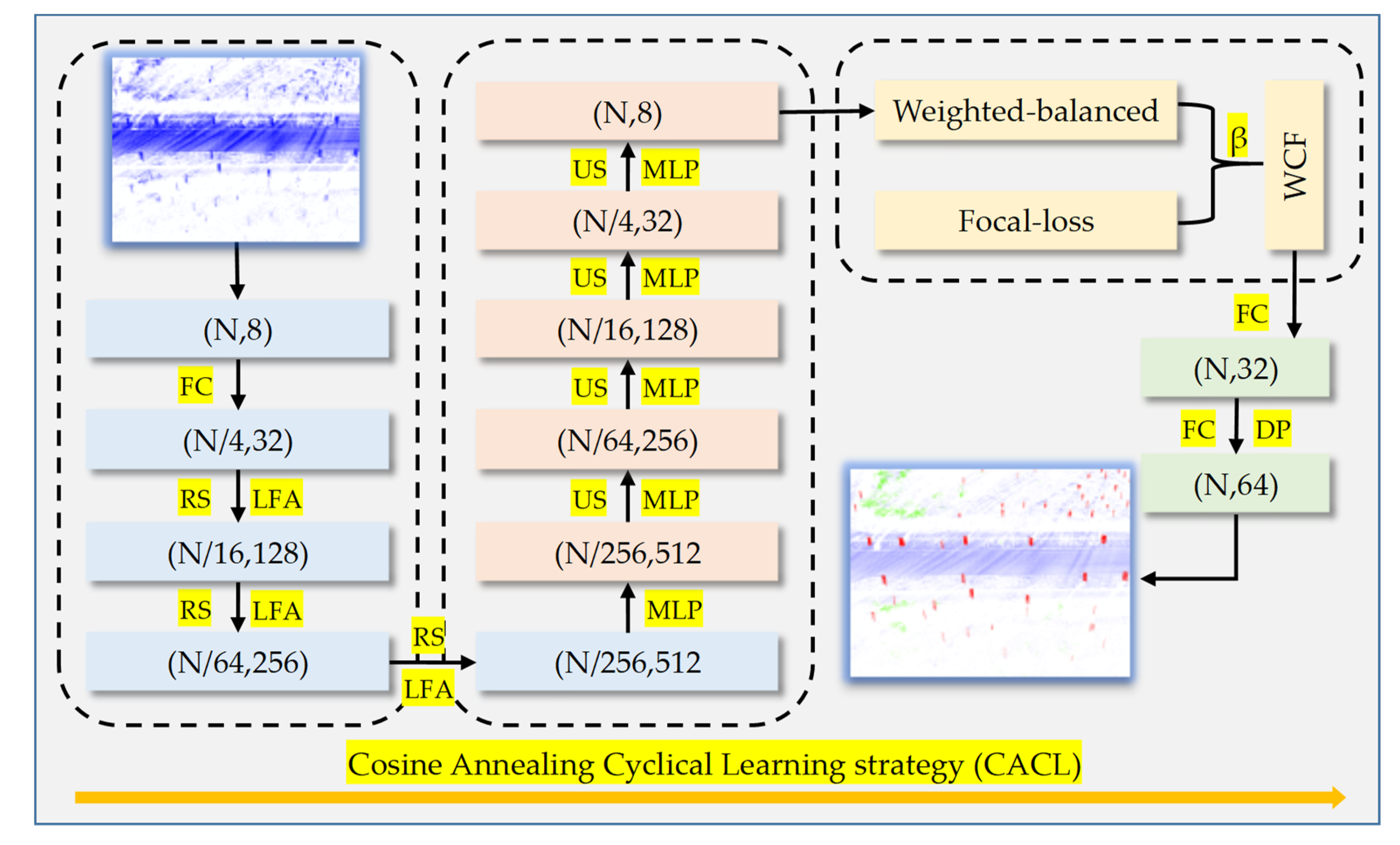
In this study, the method used for tree trunk detection is the improved WCF-CACL-RandLA-Net model based on the RandLA-Net model. RandLA-Net [28] is an advanced deep learning (DL) model for large-scale point cloud semantic segmentation, which employs efficient random sampling (RS) and local feature aggregation (LFA). Its network structure is similar to the encoder–decoder network structure (first downsampling, then upsampling). To enhance the performance of the RandLA-Net model for tree trunk detection, we improved the loss function and learning strategy in RandLA-Net by introducing the weighted cross-entropy focal-loss module (WCF) and the cosine annealing cyclic learning strategy (CACL). WCF, through the integration of the weighted cross-entropy loss function (WCL) and the focal loss function (FL), strengthens the model’s generalization ability while increasing the model’s attention weight on target classes during the training process, which is beneficial for addressing class imbalance issues. CACL enables the dynamic adjustment of the model’s learning rate throughout the training process. The cyclically varying learning decay strategy significantly enhances the exploration of model parameters, helps the model escape local optima, and avoids overfitting during training. Figure 6 displays the network framework of the WCF-CACL-RandLA-Net model.
(1)
Weighted Cross-Entropy Focal-Loss (WCF)
The dataset used for tree trunk detection exhibits features such as class imbalance and a smaller proportion of target classes. The weighted cross-entropy loss function employed by RandLA-Net is insufficient to focus on less represented classes. In the training samples of this study, the target point cloud accounts for 3% of the total number of point clouds trained. To address this issue, we proposed a loss function that combines weighted cross-entropy loss and focal loss to enhance the model’s focus on underrepresented classes.
Weighted cross-entropy loss is a variation of the standard cross-entropy loss function, adjusting the importance of each class in loss computation by assigning different weights to different classes. Focal loss is a loss function designed to address the class imbalance by introducing a modulating factor that increases the loss of difficult-to-classify samples, thereby making the model more attentive to these challenging samples. We combine weighted cross-entropy loss and focal loss to form a new loss function (WCF).
L C E = i = 1 N c = 1 C W c × Y i c × l o g P i c
L F L = i = 1 N c = 1 C Y i c × 1 P i c γ × l o g P i c
L = 1 β × L C E + β × L F L
In the formula, “ N ” represents the number of point clouds; “C”represents the number of classes; “ W c ” represents the weight of class “C”; “ Y i c ” represents the actual label count of point cloud “ i ” belonging to class “C”; “ P i c ” represents the predicted probability of point cloud “ i ” belonging to class “C”; “ γ ” represents the modulating factor, used to control the weight of easy and difficult samples; “ L C E ” represents weighted cross-entropy loss; " L F L ” represents focal loss; and “ β ” represents the weight coefficient. By adjusting “ β ”, we can find the optimal balance point between the two loss functions.
WCF can mitigate class imbalance issues and enhance the performance of the model when dealing with datasets exhibiting different class distribution characteristics. It takes full advantage of weighted cross-entropy loss and focal loss. Finally, by adjusting the weight coefficient “ β ” and the modulating factor “ γ ”, the performance of the RandLA-Net can be further optimized.
(2)
Cosine Annealing Cyclic Learning Strategy (CACL)
RandLA-Net employed a fixed linear decay learning strategy. Although this approach helped the model converge quickly in the early stages of training, it sometimes led to the model becoming trapped in local optima during the later stages, thereby affecting its generalization ability. To address this issue, this study introduced the cosine annealing cyclic learning strategy (CACL). CACL utilized a dynamic learning rate adjustment method, periodically adjusting the learning rate during training, enabling the model to explore the parameter space at different learning rates. Based on the cosine annealing scheduler, the learning rate fluctuated following a cosine function. CACL facilitated the RandLA-Net model’s escape from local optima, accelerated convergence speed, and reduced sensitivity to the initial learning rate and learning rate decay, rendering the model more suitable for large-scale training datasets and complex training tasks.
L R t = L R m i n + 0.5 × L R m a x + L R m i n × 1 + c o s π × t % T T
In the formula, “ L R t ” represents the learning rate at training step “t”, while “ L R m i n ” and “ L R m a x ” denote the minimum and maximum learning rates, respectively. “T” indicates the period of learning rate adjustment, with % symbolizing modulo operation.
The deep learning environment for this study included an I7-1900 processor with 32 GB of memory and an NVIDIA RTX A4000 16 G graphics card, utilizing CUDA 11.0 for GPU computing acceleration. The deep learning framework was TensorFlow-GPU 1.13.0, based on Python 3.5.6. The input TDS point number amounted to 1.27 × 10⁷. The nearest point “K” value was set to 16, the initial learning rate to 0.01, and “T” to 4. The model featured 40 epochs, with 500 steps per epoch. The values of “c” and “d” were set to 0.0001 and 0.01, respectively. Random sampling rates for each layer were (4, 4, 4, 2), and the feature dimensions were (16, 64, 128, 256, 512).

2.3.3. DBH Estimation Method Based on LSA-RANSAC

The WCF-CACL-RandLA-Net model generates classified point clouds with three types of labels. However, further processing is required for the clustering of individual tree trunk point clouds and DBH calculations. In this study, we designed and implemented the least squares adaptive RANSAC DBH estimation method (LSA-RANSAC). LSA-RANSAC is a point cloud DBH calculation method that integrates the adaptive RANSAC algorithm and least squares optimization. LSA-RANSAC can find the optimal parameters and the corresponding values within the desired range and define the error function by calculating the distance between the cylindrical model and the point cloud data to obtain the best-fitting cylindrical model. LSA-RANSAC takes full advantage of the robustness of the RANSAC algorithm [3] in handling noise and outliers, as well as the parameter search capability and model error convergence of adaptive methods and least squares optimization algorithms, making the entire fitting process more stable and efficient. The implementation steps of DBH calculation based on LSA-RANSAC are as follows:
Step 1: Implement the density-based spatial clustering of applications with noise (DBSCAN) [29] without specified cluster numbers by setting the minimum number of cluster points (Min-Pts) and neighborhood radius (Eps) parameters.
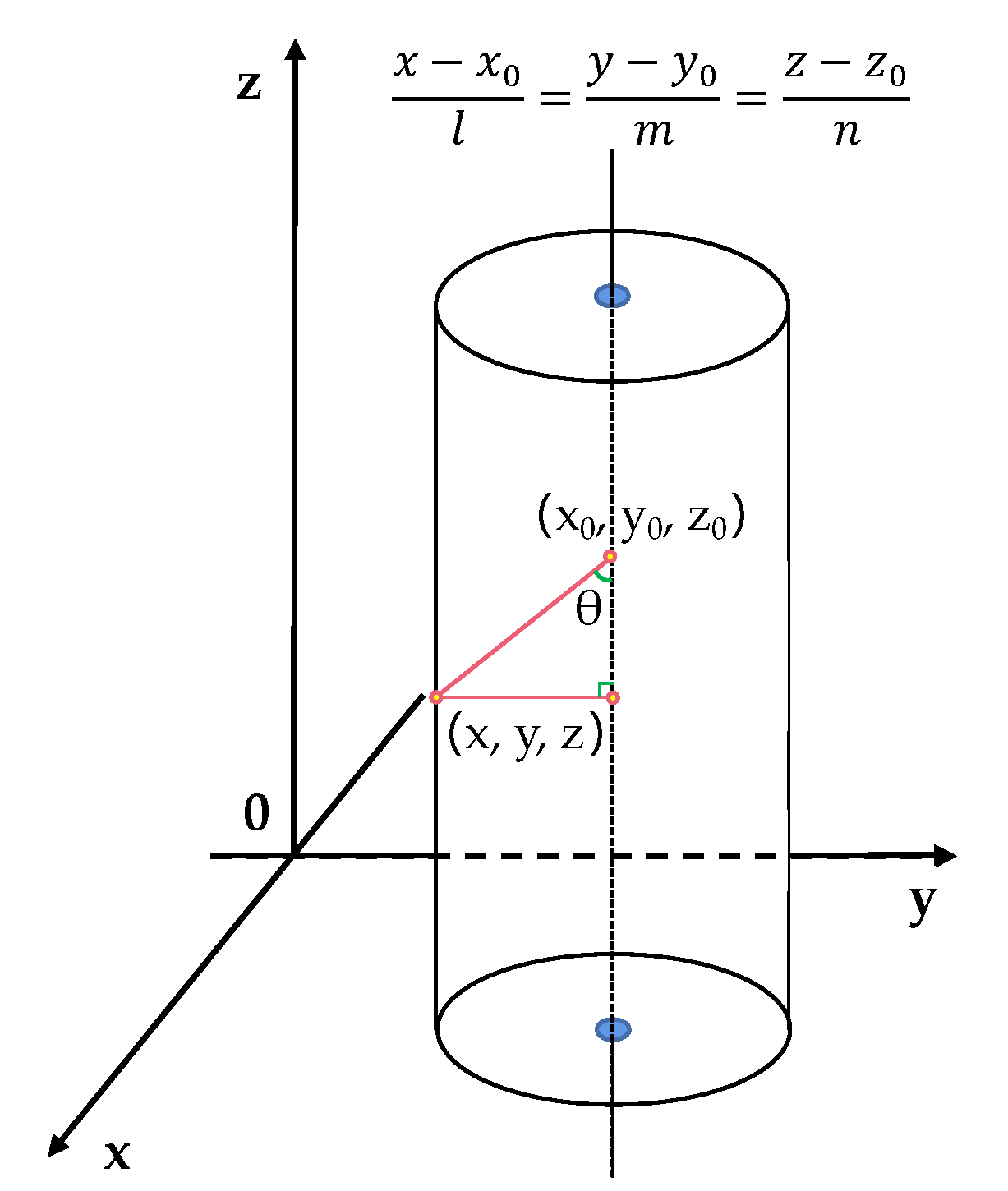
Step 2: Fit each tree trunk class using the LSA- RANSAC algorithm. First, determine the use of cylinders for DBH fitting. The equation for the fitted cylindrical model is given in Formula 9. Figure 7 illustrates the spatial schematic of the fitted cylinder.
X X i 2 + Y Y i 2 + Z Z i 2 r 2 = L × X X i + M × Y Y i + N × Z Z i 2 L 2 + M 2 + N 2
In the formula, (X, Y, Z) represented a point on the fitted cylindrical axis; (L, M, N) was the vector in the L direction of the cylindrical axis; and “r” was the radius of the circle. The cylindrical equation could be determined by these seven parameters.
The iterative fitting process of the LSA-RANSAC for the cylindrical model was as follows:
(1)
Initialize parameters: the maximum distance from the point cloud to the model, the desired inlier probability, maximum iterations, and minimum inlier count were set. The best initial inlier count and the best initial model were initialized;
(2)
Calculate the sample size based on the desired inlier probability;
(3)
Determine the best initial model parameters iteratively: randomly select a sample point cloud from the point cloud according to the current sample size. The cylindrical model was fit using the selected sample point cloud, returning the model parameters and inlier indices. The inlier count was calculated and compared with the current best initial inlier count. If the inlier count was greater than the current best initial inlier count, the best initial inlier count, the best initial model, sample size, and iteration count were updated. The adjustment process adaptively updated the sample size and iteration count based on the current inlier count;
(4)
Extract the best initial model parameters, I M p a r a m s : obtain the center point, axis direction, radius, and height of the cylinder from the best initial model acquired by the adaptive RANSAC algorithm;
(5)
Define the fitting error function by calculating the distance between the best initial model parameter I M p a r a m s and the point cloud data;
(6)
Perform nonlinear least-squares optimization on I M p a r a m s , using the Levenberg–Marquardt optimization method to solve for the minimum value of the fitting error function and obtain the best-fit cylindrical model parameters.
I M p a r a m s = a r g m a x   i = 1 n w i × p i X i θ
B M p a r a m s = a r g m i n i = 1 n ( X i - C × V r 2
In the formula, “ I M p a r a m s ” represented the best cylindrical model parameters, “ n ” represented the number of sample points, “ X i ” represented the ith point in the point cloud, “ w i ” represented the weight of the sample point, “ p i X i θ ” represented the probability of the sample point “ X i ” being fitted by the cylindrical model “ θ ”. “C” represented the center point of the cylinder; “ V ” represented the axis direction of the cylinder, and “ r ” represented the radius of the cylinder. The final result was to find the best cylindrical parameter B M p a r a m s   that minimized the sum of distances from all points to the cylinder surface.
Throughout the experiment, the segmented trunk point cloud results were used as input data. “Min-Pts” was set to 50, and “Eps” was set to 0.2. The maximum distance was set to 0.01; the desired probability was set to 0.50. The iteration count was capped at a maximum of 100, and concurrently, the floor for the inlier count was established at 15.

2.4. Comparison Method

The BSTDF framework primarily consists of two parts: tree trunk detection and DBH fitting. In this study, the KPConv [25], RandLA-Net [28], PointNet++ [30], and (the tree trunk extraction method based on vector features) VF [18] were chosen as the comparison method for the WCF-CACL-RandLA-Net model tree trunk detection deep learning model, utilizing the training samples from Section 2.3.1 for synchronous detection. Simultaneously, we chose locally optimal RANSAC [3], LS [11,12], and CHA [11] as the comparative method for LSA-RANSAC to estimate DBH. RANSAC achieves local optimality by iteratively selecting the cylindrical fitting model with the highest number of inliers. Consistent data is maintained throughout the entire fitting experiment process. The accuracy results are the average of three repeated experiments.

3. Results

3.1. Segmentation Results of Point Cloud Based on WCF-CACL-RandLA-Net Model

3.1.1. Evaluation Metrics

To assess the performance of RandLA-Net in trunk segmentation, we employed four overall benchmark metrics, including overall accuracy (OA), intersection over union (IoU), F1 Score (F1), and tree trunk detection rate (ER) to evaluate segmentation accuracy. “TP”, “TN”, “FP”, and “FN”, denoted true positives, true negatives, false positives, and false negatives, respectively. “n” represented the number of detected tree trunks, and “N” represented the actual number of surveyed trees in the sample plot.
O A = T N + T P T P + F N + T N + F P
I o U = T P T P + F P
R = T P T P + F N
F 1 = 2 × I o U × R I o U + R
E R = n N × 100 %

3.1.2. Training Loss and Elapsed Time

During the training process of deep learning algorithms, we used training accuracy and loss functions to assess the convergence of the model training process, which might also reflect the error between the final segmentation results of the point cloud segmentation model and the true values. Figure 8A illustrates the increase in training accuracy over time. After 40 training iterations, both WCF-CACL-RandLA-Net and RandLA-Net training accuracies stabilized between 0.99 and 1.00. Within the same training duration, WCF-CACL-RandLA-Net demonstrated higher training accuracy and better convergence than RandLA-Net. Figure 8B depicts the change in loss functions for both models during the training period. As the models were trained, the loss functions gradually converged, and after 40 training iterations, the training losses for both models stabilized between 0 and 0.05. The WCF-CACL-RandLA-Net training process required 3 h and 2 min, while the RandLA-Net model training process took 3 h, indicating that WCF and CACL did not increase the training burden.

3.1.3. Quantitative and Qualitative Evaluation

As previously mentioned, Table 2 displays the quantitative and visual inspection evaluation results of the tree trunk detection process for both models. The OA, IoU, and F1 for the WCF-CACL-RandLA-Net model were 0.98, 0.88, and 0.92, respectively. Compared to RandLA-Net, the OA of the WCF-CACL-RandLA-Net model did not change significantly due to the point cloud count of the ground category accounting for over 80% of the total category point cloud count. However, the segmentation accuracy metrics IoU increased from 0.85 to 0.88, and F1 increased from 0.90 to 0.92, achieving higher segmentation accuracy; particularly for Tree-trunk and Shrubs-branches, the segmentation accuracy improved by 6% and 5%, respectively, while F1 increased by 3% for both. The aforementioned results indicate that the WCF effectively improved the segmentation accuracy of the RandLA-Net model when processing imbalanced the point cloud datasets. During the training process, the WCF module emphasized the model’s attention to trunk class point clouds, helping the model to perform well in identification and localization tasks even in sparse and occluded situations, thus, making the model’s segmentation accuracy more balanced and enhancing its generalization ability. Simultaneously, CACL allowed the model to have more flexible learning rate variation and parameter exploration capabilities; through end-to-end training, it improved the segmentation performance of the RandLA-Net model for objects easily confused between trunks and leaves.

3.1.4. Comparative Studies

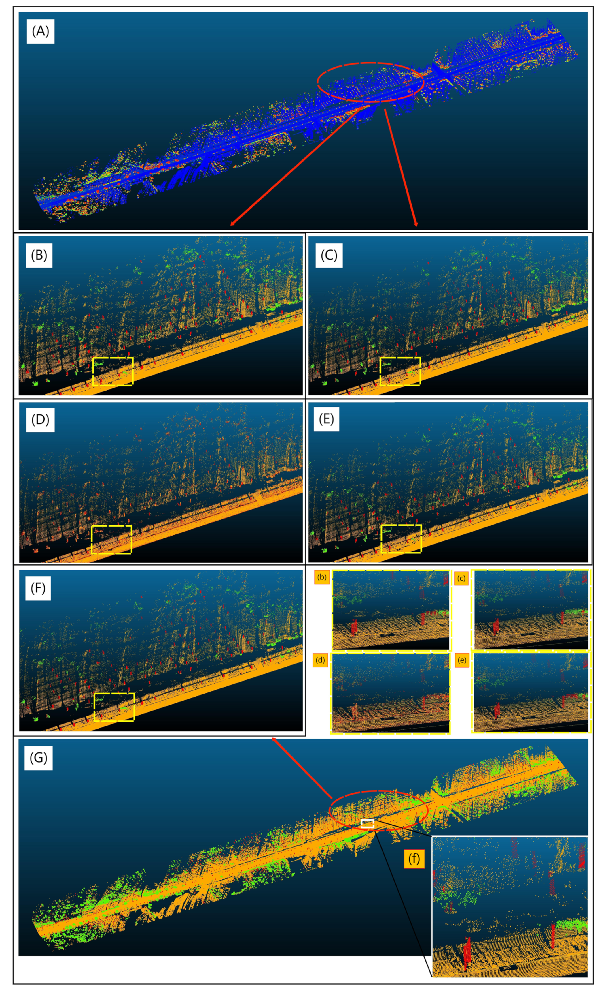
In order to demonstrate the efficacy of the proposed method qualitatively for segmenting tree trunks within complex forest MLS point cloud scenarios, we designed a number of experiments and compared it with selected popular methods, including one traditional method (VF) [18] and three deep learning approaches (KPConv [25], RandLA Net [28], and PointNet++ [30]). We tabulated the precision results of various methods in Table 3, with selected visual result examples showcased in Figure 9. Notably, our proposed method currently registered the highest mIoU score of 0.89, followed by RandLA-Net, trailing by roughly 4%. KPConv sat slightly below RandLA-Net by around 2%, with the lowest trunk segmentation precision attributed to PointNet++. It is worth emphasizing that all four aforementioned methods substantially outperformed traditional feature vector-based trunk detection methods.All deep-learning methods delivered satisfactory results for tree trunk point clouds with pronounced trunk shapes. However, for complex location distributions, such as scenarios where multiple trees are distributed in queues with severe spatial overlap, both PointNet++ and KPConv tended to generate omissions in trunk detection, often misclassifying surrounding branches and leaves as trunks. While RandLA-Net does show some improvement in reducing trunk omission errors, the misclassification of branches and leaves as trunks still remains prevalent. The training and testing duration for PointNet++ and KPConv outlasts that of RandLA-Net and WCF-CACL-RandLA-Net. The traditional method, although quick, is plagued by severe omissions or debugging errors, primarily due to its strong dependence on the integrity of the tree trunk annular point cloud and the spatial features of adjacent woods. The network structure and parameters of deep learning methods are able to implicitly articulate the spatial interactions between trunks, branches, leaves, and ground point clouds, facilitating feature representation, such as segmentation. Despite the added computational complexity introduced by deep learning methods, such shifts should be tolerated when performing trunk extraction and DBH estimation in large-scale MLS point clouds [20].

3.1.5. Ablation Experiments

In the forthcoming experiments, we delved into the influence of the weighted cross entropy focal loss function module (WCF) and the cosine annealing cycle learning strategy (CACL) on the segmentation precision of the RandLA-Net model during the process of tree trunk identification, leveraging the technique of ablation studies. Empirical findings highlight the positive contributions of both WCF and CACL to the segmentation capabilities of the RandLA-Net model. As illustrated in Table 4, during the segmentation of the hierarchically-coupled tree trunk identification dataset, WCF effectively mitigated discrepancies in segmentation precision induced by imbalanced point cloud class quantities. With the utilization of the WC-RandLA-Net, the recognition precision for tree trunks and shrubs within the point cloud data eclipsed the standard RandLA-Net model by 5% and 3%, respectively. Moreover, when the mean intersection over union (IoU) exceeded 80%, the step count amounted to 2000 and 3500 for the CACL-RandLA-Net and the RandLA-Net, respectively. This evidence corroborates the notion that CACL accelerates the convergence of deep learning models and exerts a propitious influence on segmentation precision.

3.1.6. Impact of Laser Scanning Distance Level on Tree Trunk Detection Rate (ER)

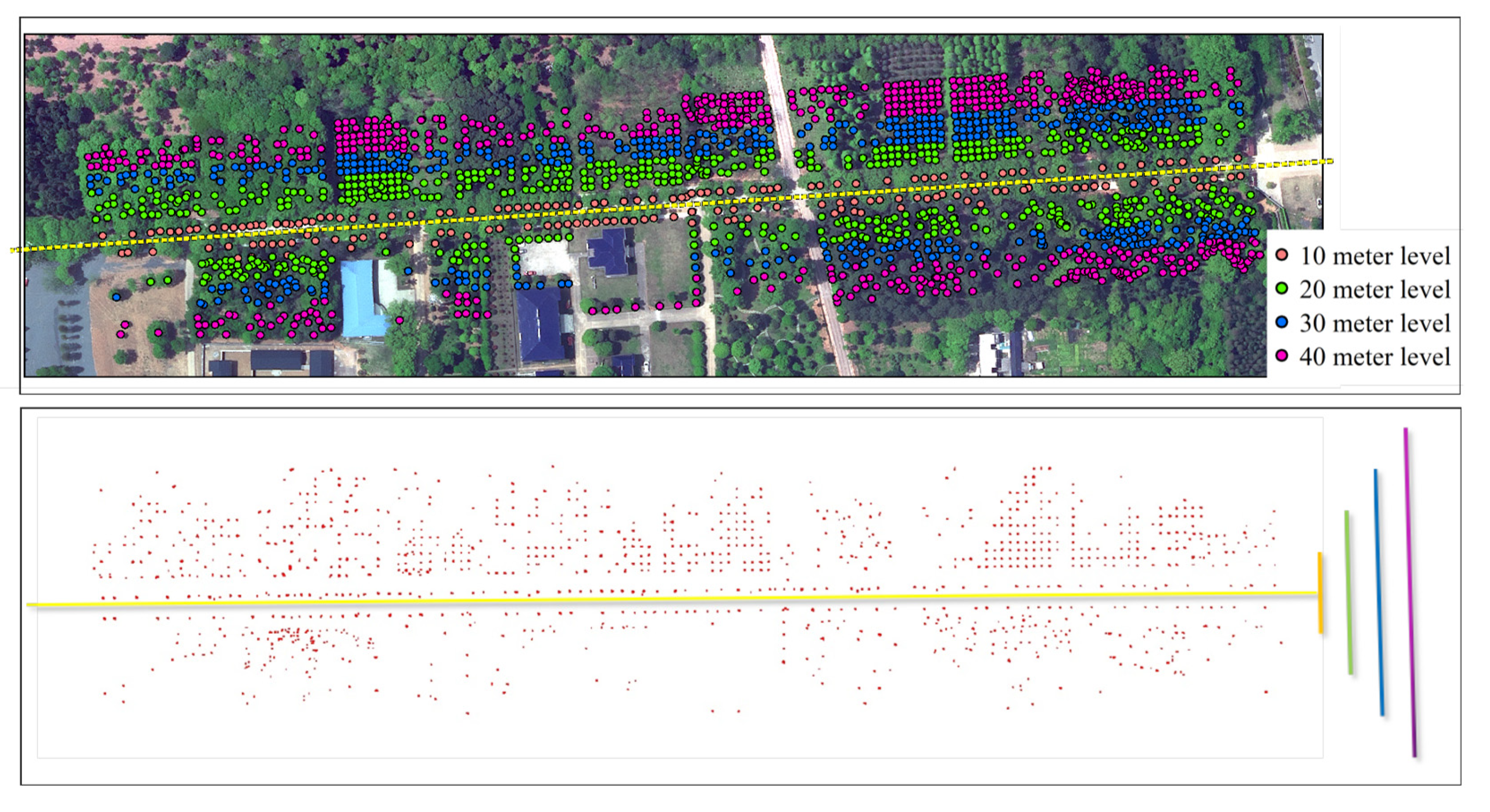
Similar to other tree trunk detection segmentation methods [8,9,15,16], irregular trunk shapes and point cloud scarcity caused by obstacles and laser scanning distance in the forest remain the primary factors affecting accurate measurements [23,31,32]. To determine the impact of scanning distance on ER, we divided trees into four distance levels (0–10 m, 10–20 m, 20–30 m, and 30–45 m) based on the horizontal distance between the trees and the scanning path (Figure 10) and compared the ER values within different distance levels. The results, as shown in Table 5, indicated that ER decreased as the distance level increased. The closer the samples were to the scanning path, the higher the ER value. The ER values for the 10 m, 20 m, 30 m, and 40 m levels were 97.70%, 83.36%, 68.09%, and 32.47%, respectively, with an average ER of 70.41%. The distance level with an ER above 80% was 20 m, and the average ER value at this distance level was 90.53%. Increasing the density of the LiDAR scanner’s path in the forest was an effective way to improve ER values. Considering accuracy and efficiency, we recommend that the BLS data collection distance level for tree trunk detection and recognition should not exceed 20 m, and the optimal bandwidth (the parallel distance between two adjacent scanning paths) of multiple parallel paths should not exceed 40 m.

3.2. DBH Estimation Results Based on LSA-RANSAC

3.2.1. Evaluation Metrics

The evaluation metrics for DBH fitting accuracy are the coefficient of determination (R2), root mean square error (RMSE), and residuals between measured and estimated values (Residual).
R 2 = 1 i = 1 n R 2 i = 1 n y i y ¯ 2
R M S E = 1 n y i y i ^ 2 n
R e s i d u a l = y i y i ^
In the formula, “ y i ” represents the ith measured value, “ y i ^ ” represents the ith predicted value, “ y ¯ ” represents the average measured DBH, and “ n ” represents the number of detected trunks.

3.2.2. Fitting Accuracy Comparison

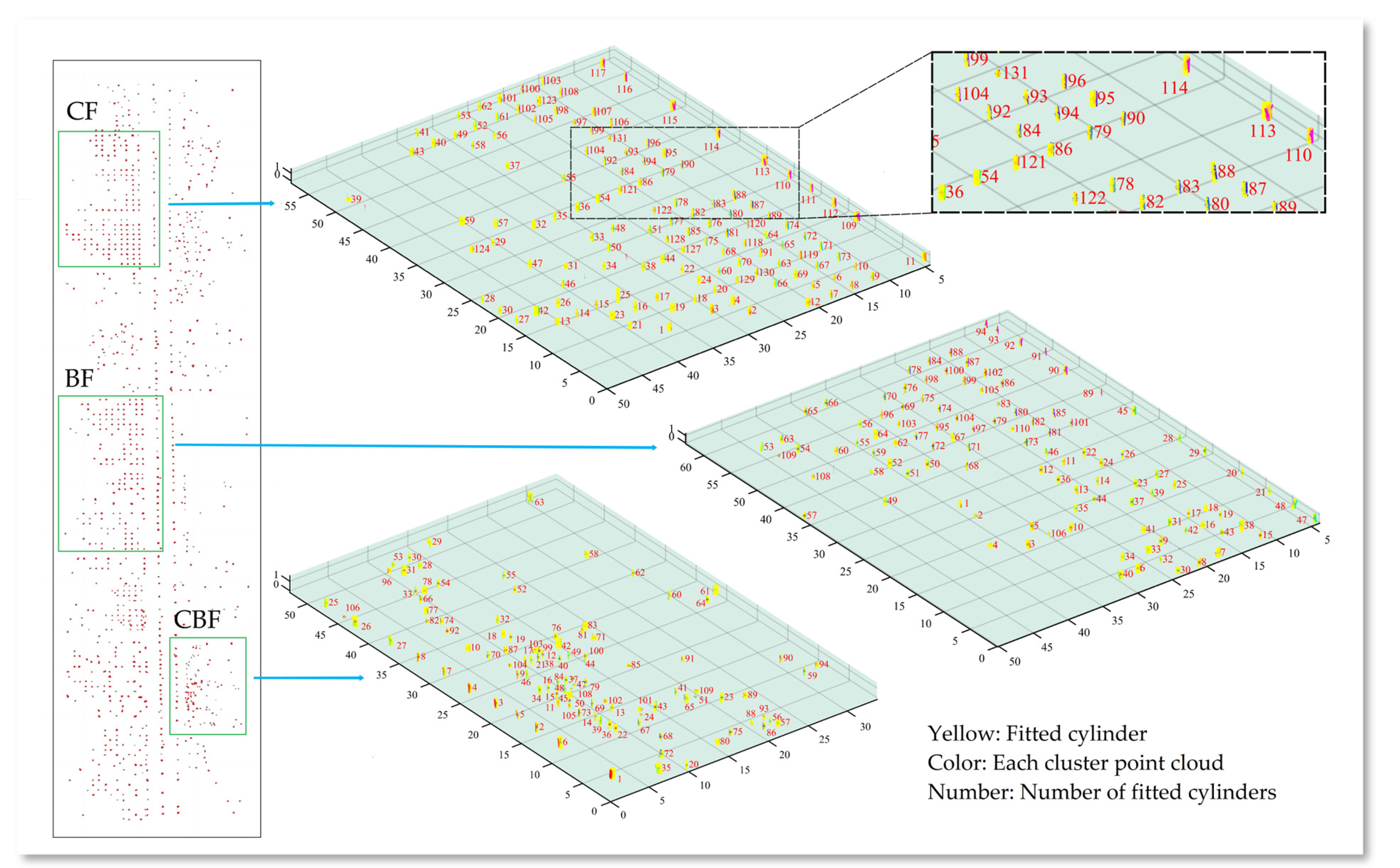
To verify the accuracy and effectiveness of the DBH estimation results, three subplots were set up within the plot area (Figure 11), including a coniferous forest sampling plot (CF: 50 m × 60 m), a broadleaf forest sampling plot (BF: 50 m × 60 m), and a coniferous-broad mixed forests sampling plot (CBF: 40 m × 60 m). The closure degrees of the three subplots were 0.90, 0.85, and 0.95, respectively, with a stand density of 666.7 trees/ha, 426.6 trees/ha, and 504 trees/ha. The DBH fitting results of all trees within the three subplots (Figure 11) were statistically analyzed (Table 6). The statistics showed that the coefficient of determination (R2) for the LSA-RANSAC based DBH estimation was 0.77, 0.74, and 0.73, with RMSE values of 6.37 cm, 6.20 cm, and 6.92 cm. The residual values of all sample plots were uniformly distributed around the X-axis (Figure 12). In well-distributed coniferous and broadleaf forests, DBH estimation accuracy was higher than in randomly distributed mixed forests. The DBH estimation accuracy in coniferous forests was slightly higher than in broadleaf forests, which might be due to some trunks in broadleaf forests having bifurcations, causing cylinder overfitting and affecting DBH estimation accuracy. Compared to RANSAC, the average R2 of LSA-RANSAC increased by 14%, and the average RMSE decreased by 1.08 cm. The lower DBH estimation accuracy of the RANSAC method was due to widespread cylinder underfitting. The LSA-RANSAC method effectively reduced error values during fitting by iteratively updating the selection of points and inliers and constraining the objective function of cylinder parameters, thus improving the DBH fitting accuracy of the RANSAC method. Although LSA-RANSAC showed effectiveness in DBH estimation, we still compared it with the least squares (LS) [11,12] and convex hull (CHA) [11] fitting methods. It is worth noting that the cylindrical fitting method based on RANSAC was generally significantly superior to the CHA and LS methods for estimating chest diameter. This is because the CHA and LS methods were more sensitive to missing cylindrical point clouds.

3.2.3. Analysis of Tree Trunk Detection Accuracy Based on LiDAR Scanning Distance Level

To evaluate the impact of scanning distance on DBH estimation, the estimated DBH values of the three subplots using LSA-RANSAC were statistically analyzed according to the distance level (Table 7), and the estimation accuracy of the DBH at different distance levels was compared. In the three forest types, the distance levels with DBH estimation accuracy above 80% were 30 m for the coniferous forest, 20 m for the broadleaf forest, and 10 m for the coniferous–broadleaf mixed forest. The DBH estimation accuracy in the mixed forest subplot was lower than that in the coniferous and broadleaf forest subplots due to the uniform distribution of trees in the coniferous and broadleaf forest subplots, while the trees in the broadleaf forest subplot were densely and centrally distributed. Overall, the R2 of the DBH values estimated by the LSA-RANSAC method was negatively correlated with the LiDAR scanning distance level, while the RMSE was positively correlated. The average DBH estimation accuracy for the three forest types at distance levels within 20 m was above 80%. Within the 0–20 m range, the R2 was 0.87, and the RMSE was 4.41 cm. Taking accuracy and efficiency into consideration, we also recommend that the range of BLS data collection for DBH estimation should not exceed 20 m, and the optimal bandwidth for multiple parallel paths should not exceed 40 m.

4. Discussion

In this study, we focused on the importance of accurate assessment and scientific management of forest resources in the context of exacerbated global climate change and ecological environmental issues. We combined remote sensing technology and computer algorithms to propose a novel framework for forest tree trunk detection and DBH estimation based on BLS, called the BLS-based tree-trunk detection framework (BSTDF). Firstly, we created a reusable tree trunk detection deep learning dataset using a stratified coupling method. Secondly, we improved the learning strategy and loss function of the RandLA-Net model to adapt to tree trunk detection tasks in large-scale forests and address the issue of class imbalance in segmentation. Lastly, we introduced the LSA-RANSAC method to enhance the accuracy of DBH estimation. The effectiveness of the BSTDF was validated in a 65,000 m2 forest at the Subtropical Forestry Experiment Center of the Chinese Academy of Forestry Sciences.
To fully harness the potential of mobile laser scanning (MLS), one of the primary focuses of this research lies in the construction of a tree trunk detection dataset for deep learning. In previous studies [20,23,25,33], the datasets used for forest point cloud segmentation predominantly comprised entire forest trees. While not all researchers regard direct segmentation of complete forest scenes as unacceptable, reducing the quantity of non-target point clouds is vital to enhancing segmentation efficiency and accuracy. Accordingly, we have adopted a novel hierarchically-coupled method to establish a dataset suitable for tree trunk detection based on deep learning. By dividing the full forest point cloud into four strata: ground point cloud layer (0.0 m to 0.1 m), non-target point cloud layer 1 (0.1 m to 1.0 m), target point cloud layer (1.0 m to 1.6 m), and non-target point cloud layer 2 (1.6 m and above), we couple the ground layer and target trunk layer based on coordinate calculations, thus, forming the foundational dataset for trunk detection. This data processing method dramatically trims the data volume within the detection point cloud, enhancing the learning efficiency of deep learning algorithms and providing substantial reference value in dataset creation.
In this study, we used the improved WCF-CACL-RandLA-Net model, which is suitable for large-scale point cloud segmentation, for tree trunk detection. Compared to other deep learning models [23,24,25,26,27], the RandLA-Net model employs a random sampling (RS) method that can process one million points at a time, and through the LFA structural design, it achieves aggregation of local features. This overcomes the problem of insufficient sparse keypoints information caused by RS. The study findings reveal that KPConv is marginally inferior to RandLA-Net by approximately 2%, with PointNet++ falling short in terms of trunk segmentation precision. These observations resonate with the findings of Wang et al. [20] and Hu et al. [28,34], who found RandLA-Net’s segmentation prowess outshone other leading semantic segmentation methods. By introducing the WCF and CACL, the WCF-CACL-RandLA-Net model demonstrates better performance in tree trunk detection tasks compared to the RandLA-Net model. Firstly, the introduction of the WCF enables the model to learn trunk features more effectively, which helps eliminate the impact of point cloud noise and occlusion and improves tree trunk detection accuracy. Secondly, the introduction of the CACL helps the model adaptively adjust the learning rate during training, ensuring a suitable learning speed at different stages. This helps to avoid the model falling into local optima and enhances its generalization performance.
Traditional trunk detection methodologies, such as those reliant on vector features (VF) [18,19], geometric circle fitting [35], cylinder fitting [36], and cross-section detection [37], are excessively sensitive to incomplete trunk point clouds and lack robustness. In contrast, deep learning algorithms demonstrate notable superiority in detection accuracy. For instance, our framework method outperforms VF in trunk point cloud recognition precision by 48%. Moreover, our approach exhibits greater robustness when handling large-scale forest data without necessitating point cloud-raster data conversion [37] or manual elimination of non-target point clouds. In addition, compared to other deep learning-based improved methods, our model shows higher accuracy and stability in tree trunk detection tasks, with an IOU segmentation accuracy of 0.88 for the hierarchically coupled data layer, which is superior to the segmentation performance of RandLA-Net on other datasets [29,37]. In future research, we may consider further enhancing the model’s performance in handling large-scale tree trunk detection tasks by improving the model structure or employing distributed computing techniques.
Of course, the fitting method for DBH also affects the accuracy of DBH estimation. In previous studies [12,13,14,38], circle fitting-based DBH estimation has developed into a mature approach. Different methods have their respective strengths and weaknesses. Least squares (LS) [11,12] can achieve satisfactory fitting results when processing simple and regular point clouds, but its ability to handle outliers is limited. Hough transform (HT) [14] has a high computational complexity, is sensitive to parameters, and requires manual selection of appropriate parameters, resulting in limited robustness. The convex hull algorithm (CHA) [11] may perform poorly when processing data from densely populated forest areas and is susceptible to noise and occlusion. RANSAC [3] has certain advantages in handling noise and occlusion issues but requires manual parameter settings, such as inlier threshold and iteration count, and is sensitive to parameter selection. In view of these shortcomings, this research proposes a LSA-RANCAC method. The experimental results show that this method combines the fitting accuracy of the least squares method with the robustness of the RANSAC method, providing a strong outlier processing capability, adaptive parameter settings, and high fitting accuracy, which is significantly better than RANSAC, LS, and CHA fitting methods. Of course, there is still room for improvement in the LSA-RANSAC method used in this study. For example, Duanmu, J. et al. [2] proposed an adjacent point distribution analysis (ANPDA) method to reduce noisy point clouds, which could be an effective way to further enhance the LSA-RANSAC method.
In this study, the forest stand density of our test area was set at 394 stems per hectare, and 1270 trees were detected using our method. When the LiDAR scanning distance level was set at 20 m, the average ER was 90.03%, significantly higher than the 17.4–32% reported in other studies [2,11]. Considering the three forest types established in this study—mixed coniferous, mixed broadleaf, and mixed coniferous–broadleaf forests—the forest type also has an impact on the accuracy on BLS-based DBH estimation. The trunk extraction and fitting accuracy of mixed coniferous and mixed broad-leaved forests are higher than that of mixed coniferous and broad-leaved forests, possibly due to higher spatial clustering and wider diameter distribution in mixed coniferous–broadleaf forests. If the accuracy of individual tree trunk detection is guaranteed, BLS will be the most suitable solution for estimating mountain forest parameters. This is because BLS offers greater portability and excellent penetration capabilities, with the highest accuracy in the main tree trunk detection and DBH estimation through a single scan [5,39].

5. Conclusions

This study presented a novel framework for forest tree trunk detection and DBH estimation based on BLS (BSTDF), aimed at addressing the difficulty and low accuracy of obtaining large-scale forest DBH information. In BSTDF, a stratified coupling method using BLS was employed to construct a tree trunk detection dataset, significantly reducing the dataset size, improving computational efficiency, and enhancing the generalization capability of deep learning models. BSTDF improved the RandLA-Net deep learning algorithm by introducing WCF and CACL, effectively mitigating class imbalance issues in the tree trunk detection process, accelerating model convergence, and enhancing model stability and accuracy. Furthermore, BSTDF estimated DBH by using the cylindrical fitting method of LSA-RANSAC, fully leveraging the parameter search capabilities of adaptive methods and least squares optimization algorithm, and model error convergence, making the entire DBH fitting process more accurate. The experimental results showed that the OA, IoU, and F1 of the WCF-CACL-RandLA-Net model were 0.98, 0.88, and 0.92, respectively. Better than segmentation algorithms such as KPConv, PointNet++, and VF. Compared to RandLA-Net, the IoU increased from 0.85 to 0.88, and the F1 increased from 0.90 to 0.92. Particularly, the segmentation accuracy of the trunk category improved by 6%, and the F1 increased by 3%, effectively addressing the class accuracy imbalance issue when RandLA-Net segmented trunks. The overall tree trunk detection rate was 70.41%. RMSE and R2 for the overall DBH estimation accuracy of LSA-RANSAC were 6.50 cm and 0.75, respectively. Compared to RANSAC, RMSE decreased by 1.08 cm, and R2 increased by 14%, indicating that LSA-RANSAC effectively mitigated RANSAC’s underfitting problem and improved DBH estimation accuracy. Both ER and DBH estimation accuracy were negatively correlated with the LiDAR scanning distance (bandwidth). Considering the accuracy and efficiency, the optimal distance level for single-path BLS data collection was 20 m, and the optimal scanning bandwidth for multiple parallel paths should not exceed 40 m. Under these conditions, the average ER of BSTDF was 90.03%, with a DBH estimation accuracy of RMSE 4.41 cm and R2 0.87.
In conclusion, the BSTDF provided effective technical support for large-scale forest trunk identification and DBH estimation. We recommended applying the proposed method in other forests to evaluate its performance and limitations when encountering different environments. Additionally, by testing under various terrain conditions, BSTDF could be further optimized and improved, making it more versatile and adaptable.

Author Contributions

Conceptualization, H.Z. (Huacong Zhang) and H.Z. (Huaiqing Zhang); methodology, H.Z. (Huacong Zhang) and H.Z. (Huaiqing Zhang); software, H.Z. (Huacong Zhang); validation, H.Z. (Huacong Zhang); formal analysis, H.Z. (Huacong Zhang); investigation, K.X., Y.L., and L.W.; resources, H.Q. and L.Y.; data curation, H.Z. (Huacong Zhang); writing—original draft preparation, H.Z. (Huacong Zhang); writing—review and editing, H.Z. (Huaiqing Zhang); visualization, K.X. and R.L.; supervision, H.Z. (Huaiqing Zhang) and Y.L.; project administration, H.Z. (Huaiqing Zhang); funding acquisition, H.Z. (Huaiqing Zhang). All authors have read and agreed to the published version of the manuscript.

Funding

This research was funded by the Fundamental Research Funds of Chinese Academy of Forestry (CAF), grant number CAFYBB2021ZE005, CAFYBB2019SZ004.

Data Availability Statement

Not applicable.

Acknowledgments

This work is supported by Artificial Intelligence and Visualization Team in IRIFIT, CAF. Special thanks to the teammates at the Experimental Center of Subtropical Forestry for their assistance in collecting and processing field data.

Conflicts of Interest

The authors declare that there are no conflict of interest.

References

  1. Liu, C.; Xing, Y.; Duanmu, J.; Tian, X. Evaluating Different Methods for Estimating Diameter at Breast Height from Terrestrial Laser Scanning. Remote Sens. 2018, 10, 513. [Google Scholar] [CrossRef] [Green Version]
  2. Duanmu, J.; Xing, Y. Annular Neighboring Points Distribution Analysis: A Novel PLS Stem Point Cloud Preprocessing Algorithm for DBH Estimation. Remote Sens. 2020, 12, 808. [Google Scholar] [CrossRef] [Green Version]
  3. Olofsson, K.; Holmgren, J.; Olsson, H. Tree Stem and Height Measurements using Terrestrial Laser Scanning and the RANSAC Algorithm. Remote Sens. 2014, 6, 4323–4344. [Google Scholar] [CrossRef] [Green Version]
  4. Brede, B.; Lau, A.; Bartholomeus, H.M.; Kooistra, L. Comparing RIEGL RiCOPTER UAV LiDAR Derived Canopy Height and DBH with Terrestrial LiDAR. Sensors 2017, 17, 2371. [Google Scholar] [CrossRef] [Green Version]
  5. Oveland, I.; Hauglin, M.; Giannetti, F.; Schipper Kjørsvik, N.; Gobakken, T. Comparing Three Different Ground Based Laser Scanning Methods for Tree Stem Detection. Remote Sens. 2018, 10, 538. [Google Scholar] [CrossRef] [Green Version]
  6. Wang, Z.; Lu, X.; An, F.; Zhou, L.; Wang, X.; Wang, Z.; Zhang, H.; Yun, T. Integrating Real Tree Skeleton Reconstruction Based on Partial Computational Virtual Measurement (CVM) with Actual Forest Scenario Rendering: A Solid Step Forward for the Realization of the Digital Twins of Trees and Forests. Remote Sens. 2022, 14, 6041. [Google Scholar] [CrossRef]
  7. Van Leeuwen, M.; Nieuwenhuis, M. Retrieval of forest structural parameters using LiDAR remote sensing. Eur. J. For. Res. 2010, 129, 749–770. [Google Scholar] [CrossRef]
  8. Liang, X.; Kukko, A.; Kaartinen, H.; Hyyppä, J.; Yu, X.; Jaakkola, A.; Wang, Y. Possibilities of a Personal Laser Scanning System for Forest Mapping and Ecosystem Services. Sensors 2014, 14, 1228–1248. [Google Scholar] [CrossRef]
  9. Bauwens, S.; Bartholomeus, H.; Calders, K.; Lejeune, P. Forest Inventory with Terrestrial LiDAR: A Comparison of Static and Hand-Held Mobile Laser Scanning. Forests 2016, 7, 127. [Google Scholar] [CrossRef] [Green Version]
  10. Chen, S.; Liu, H.; Feng, Z.; Shen, C.; Chen, P. Applicability of personal laser scanning in forestry inventory. PLoS ONE 2019, 14, e0211392. [Google Scholar] [CrossRef]
  11. Pueschel, P.; Newnham, G.; Rock, G.; Udelhoven, T.; Werner, W.; Hill, J. The influence of scan mode and circle fitting on tree stem detection, stem diameter and volume extraction from terrestrial laser scans. ISPRS J. Photogramm. Remote Sens. 2013, 77, 44–56. [Google Scholar] [CrossRef]
  12. Calders, K.; Newnham, G.; Burt, A.; Murphy, S.; Raumonen, P.; Herold, M.; Culvenor, D.; Avitabile, V.; Disney, M.; Armston, J.; et al. Nondestructive estimates of above-ground biomass using terrestrial laser scanning. Methods Ecol. Evol. 2015, 6, 198–208. [Google Scholar] [CrossRef]
  13. Trochta, J.; Krucek, M.; Vrska, T.; Kral, K. 3D forest: An application for descriptions of three-dimensional forest structures using terrestrial lidar. PLoS ONE 2017, 12, e0176871. [Google Scholar] [CrossRef] [Green Version]
  14. Sun, H.; Wang, G.; Lin, H.; Li, J.; Zhang, H.; Ju, H. Retrieval and accuracy assessment of tree and stand parameters for chinese fir plantation using terrestrial laser scanning. IEEE Geosci. Remote Sens. Lett. 2015, 12, 1993–1997. [Google Scholar] [CrossRef]
  15. Del Perugia, B.; Giannetti, F.; Chirici, G.; Travaglini, D. Influence of Scan Density on the Estimation of Single-Tree Attributes by Hand-Held Mobile Laser Scanning. Forests 2019, 10, 277. [Google Scholar] [CrossRef] [Green Version]
  16. Angermueller, C.; Pärnamaa, T.; Parts, L.; Stegle, O. Deep learning for computational biology. Mol. Syst. Biol. 2016, 12, 878. [Google Scholar] [CrossRef]
  17. Olofsson, K.; Holmgren, J. Single Tree Stem Profile Detection Using Terrestrial Laser Scanner Data, Flatness Saliency Features and Curvature Properties. Forests 2016, 7, 207. [Google Scholar] [CrossRef]
  18. Wang, X.; Yang, Z.; Cheng, X.; Stoter, J.; Xu, Z.; Wu, Z.; Nan, L. GlobalMatch: Registration of forest terrestrial point clouds by global matching of relative stem positions. ISPRS J. Photogramm. Remote Sens. 2023, 197, 71–86. [Google Scholar] [CrossRef]
  19. Li, J.; Cheng, X.; Xiao, Z. A branch-trunk-constrained hierarchical clustering method for street trees individual extraction from mobile laser scanning point clouds. Measurement 2022, 189, 110440. [Google Scholar] [CrossRef]
  20. Wang, P.; Tang, Y.; Liao, Z.; Yan, Y.; Dai, L.; Liu, S.; Jiang, T. Road-Side Individual Tree Segmentation from Urban MLS Point Clouds Using Metric Learning. Remote Sens. 2023, 15, 1992. [Google Scholar] [CrossRef]
  21. Liu, Y.; Zhang, H.; Cui, Z.; Lei, K.; Zuo, Y.; Wang, J.; Hu, X.; Qiu, H. Very High Resolution Images and Superpixel-Enhanced Deep Neural Forest Promote Urban Tree Canopy Detection. Remote Sens. 2023, 15, 519. [Google Scholar] [CrossRef]
  22. Armitage, S.; Awty-Carroll, K.; Clewley, D.; Martinez-Vicente, V. Detection and Classification of Floating Plastic Litter Using a Vessel-Mounted Video Camera and Deep Learning. Remote Sens. 2022, 14, 3425. [Google Scholar] [CrossRef]
  23. Ning, X.; Ma, Y.; Hou, Y.; Lv, Z.; Jin, H.; Wang, Y. Semantic Segmentation Guided Coarse-to-Fine Detection of Individual Trees from MLS Point Clouds Based on Treetop Points Extraction and Radius Expansion. Remote Sens. 2022, 14, 4926. [Google Scholar] [CrossRef]
  24. Chen, X.; Jiang, K.; Zhu, Y.; Wang, X.; Yun, T. Individual Tree Crown Segmentation Directly from UAV-Borne LiDAR Data Using the PointNet of Deep Learning. Forests 2021, 12, 131. [Google Scholar] [CrossRef]
  25. Thomas, H.; Qi, R.; Deschaud, E.; Marcotegui, B.; Goulette, F.; Guibas, L. Kpconv: Flexible and deformable convolution for point clouds. In Proceedings of the IEEE/CVF International Conference on Computer Vision, Seoul, Republic of Korea, 27 October–2 November 2019; pp. 6411–6420. [Google Scholar]
  26. Aloysius, N.; Geetha, M. A Review on Deep Convolutional Neural Networks. In Proceedings of the 2017 International Conference on Communication and Signal Processing (ICCSP 2017), Chennai, India, 6–8 April 2017; pp. 588–592. [Google Scholar] [CrossRef]
  27. Lee, H.; Slatton, K.C.; Roth, B.E.; Cropper, W.P. Adaptive clustering of airborne LiDAR data to segment individual tree crowns in managed pine forests. Int. J. Remote Sens. 2010, 31, 117–139. [Google Scholar] [CrossRef]
  28. Hu, Q.; Yang, B.; Xie, L.; Rosa, S.; Guo, Y.; Wang, Z.; Trigoni, N.; Markham, A. RandLA-Net: Efficient Semantic Segmentation of Large-Scale Point Clouds. In Proceedings of the 2020 IEEE/CVF Conference on Computer Vision and Pattern Recognition (CVPR), Seattle, WA, USA, 13–19 June 2020; pp. 11105–11114. [Google Scholar]
  29. Ester, M.; Kriegel, P.; Sander, J.; Xu, X. A Density-Based Algorithm for Discovering Clusters in Large Spatial Databases with Noise; AAAI Press: Washington, DC, USA, 1996; Volume 34, pp. 226–231. [Google Scholar] [CrossRef]
  30. Qi, C.R.; Yi, L.; Su, H.; Guibas, L.J. PointNet++: Deep hierarchical feature learning on point sets in a metric space. In Proceedings of the Advances in Neural Information Processing Systems, Long Beach, CA, USA, 4–9 December 2017; pp. 5099–5108. [Google Scholar]
  31. Demol, M.; Calders, K.; Krishna Moorthy, S.M.; Van den Bulcke, J.; Verbeeck, H.; Gielen, B. Consequences of vertical basic wood density variation on the estimation of aboveground biomass with terrestrial laser scanning. Trees 2021, 35, 671–684. [Google Scholar] [CrossRef]
  32. Xu, D.; Chen, G.; Jing, W. A Single-Tree Point Cloud Completion Approach of Feature Fusion for Agricultural Robots. Electronics 2023, 12, 1296. [Google Scholar] [CrossRef]
  33. Luo, H.; Khoshelham, K.; Chen, C.; He, H. Individual tree extraction from urban mobile laser scanning point clouds using deep pointwise direction embedding. ISPRS J. Photogramm. Remote Sens. 2021, 175, 326–339. [Google Scholar] [CrossRef]
  34. Hu, Q.; Yang, B.; Khalid, S.; Xiao, W.; Trigoni, N.; Markham, A. Towards Semantic Segmentation of Urban-Scale 3D Point Clouds: A Dataset, Benchmarks and Challenges. In Proceedings of the 2021 IEEE/CVF Conference on Computer Vision and Pattern Recognition (CVPR), Nashville, TN, USA, 20–25 June 2021; pp. 4977–4987. [Google Scholar]
  35. Liang, X.; Litkey, P.; Hyyppä, J.; Matikainen, L. Automatic stem mapping using single-scan terrestrial laser scanning. IEEE Trans. Geosci. Remote Sens. 2012, 50, 661–670. [Google Scholar] [CrossRef]
  36. Dassot, M.; Constant, T.; Fournier, M. The use of terrestrial LiDAR technology in forest science: Application fields, benefits and challenges. Ann. For. Sci. 2011, 68, 959–974. [Google Scholar] [CrossRef] [Green Version]
  37. Zhang, Y.; Tan, Y.; Onda, Y.; Hashimoto, A.; Gomi, T.; Chiu, C.; Inokoshi, S. A tree detection method based on trunk point cloud section in dense plantation forest using drone LiDAR data. For. Ecosyst. 2023, 10, 100088. [Google Scholar] [CrossRef]
  38. Hackel, T.; Savinov, N.; Ladicky, L.; Wegner, J.D.; Schindler, K.; Pollefeys, M. Semantic3D.Net: A New Large-Scale Point Cloud Classification Benchmark. arXiv 2017, arXiv:1704.03847. [Google Scholar] [CrossRef] [Green Version]
  39. Giannetti, F.; Puletti, N.; Quatrini, V.; Travaglini, D.; Bottalico, F.; Corona, P.; Chirici, G. Integrating terrestrial and airborne laser scanning for the assessment of single-tree attributes in Mediterranean forest stands. Eur. J. Remote Sens. 2018, 51, 795–807. [Google Scholar] [CrossRef] [Green Version]
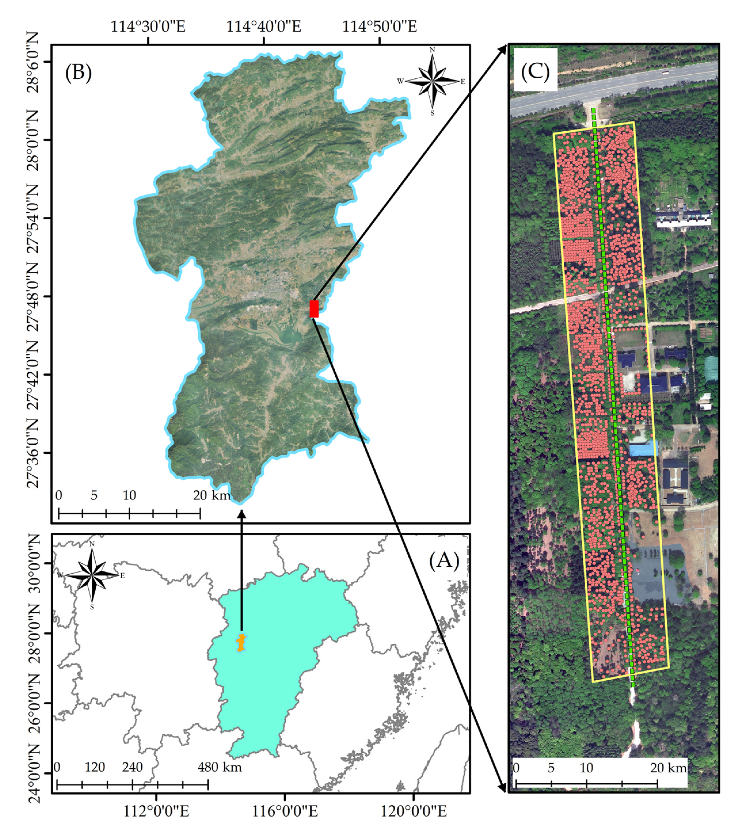
Figure 1. Study area: (A) the location of the study area in Jiangxi province; (B) the location of the study area in Fenyi County; (C) the red represents the distribution of trees, and the green dotted line represents the one-way route of LiDAR data acquisition.
Remotesensing 15 03480 g001
Figure 2. Distribution statistics of tree height and DBH of conifers and broad-leaved trees in the study area: (A) broad-leaved trees; (B) coniferous trees.
Remotesensing 15 03480 g002
Figure 3. BLS data collection equipment: (A) operation method under the forest; (B) GNNS receiver for enhanced positioning; (C) LiDAR scanner RIEGL miniVUX-1UAV; (D) point cloud in the research area.
Remotesensing 15 03480 g003
Figure 4. The flowchart of this study.
Remotesensing 15 03480 g004
Figure 5. Data processing of this study: (A,B,C) preprocessing of data; (D,E,F) stratified and coupled of data; (G) classification of the data set (the red box represents TDS; the green box represents PDS; the yellow box represents VDS).
Remotesensing 15 03480 g005
Figure 6. The network structure of WCF-CACL-RandLA-Net. (N, D) represents the number and characteristic dimension of points, respectively. FC represents the fully connected layer; LFA represents the local feature aggregation; RS represents the random sampling; MLP represents the shared multi-layer perceptron; US represents the upsampling; DP represents the dropout.
Remotesensing 15 03480 g006
Figure 7. Schematic diagram of fitting cylindrical space of LSA-RANSAC.
Remotesensing 15 03480 g007
Figure 8. The training process of two deep learning models: (A) the change process of training accuracy; (B) the training loss change process. Black represents RandLA-Net. The red color in the figure represents WCF-CACL-RandLA-Net.
Remotesensing 15 03480 g008
Figure 9. Segmentation results using different methods. Orange represents the ground, red represents the Tree-trunk category, and green represents the Shrub-branch category. (A) Point cloud to be segmented after Stratified-Coupled processing; (B,b) Segmentation results based on KPConv [25]; (C,c) segmentation results based on PointNet++ [30]; (D,d) segmentation results based on VF [18]; (E,e) segmentation results based on RandLA-Net [28]; (F,f) segmentation results based on WCF-CACL-RandLA-Net, (G) Research area segmentation results based on WCF-CACL-RandLA-Net.
Remotesensing 15 03480 g009
Figure 10. Distance level division and tree distribution map for tree trunk detection rate statistics.
Remotesensing 15 03480 g010
Figure 11. Tree distribution fitting DBH based on LSA-RANCAC.
Remotesensing 15 03480 g011
Figure 12. Comparison of the accuracy of DBH estimation results for three forest types based on LSA-RANCAC.
Remotesensing 15 03480 g012
Table 1. Descriptive statistics of field measurements (species, number, DBH, and TH) in this study.
Dataset Function Partition TypeArea (m2)Species Name of TreeNumber of TreesDBH (cm)TH (m)
MeanStdMeanStd
Training sample area19,600Yulania denudata (Desrousseaux) D. L. Fu; Magnolia officinalis Rehd.et Wils., Michelia L.; Cupressus funebris Endl.; Pinus massoniana Lamb.; Cryptomeria japonica var. sinensis Miquel.45321.349.8311.283.68
Validation sample area5000Betula luminifera H.Winkl.; Osmanthus sp., Michelia L.; Pinus massoniana Lamb.; Taxus wallichiana var. chinensis (Pilg.) Florin.22019.249.5212.336.17
Experimental sample area45,400Michelia L., Osmanthus sp.; Cinnamomum camphora (L.) presl; Nageia nagi (Thunberg) Kuntze; Taxodium distichum (L.) Rich.; Taxodium distichum var. imbricatum (Nuttall) Croom.185120.7811.2012.396.13
Total65,000Michelia L., Osmanthus sp.; Cinnamomum camphora (L.) presl; Cupressus funebris Endl.; Taxus wallichiana var.chinensis (Pilg.) Florin; Taxodium distichum (L.) Rich.230321.226.5812.763.06
Table 2. Comparison of segmentation accuracy between two deep learning models.
Classification of the Point Cloud O A I o U F 1
WCF-CACL
RandLA-Net
RandLA-NetWCF-CACL
RandLA-Net
RandLA-NetWCF-CACL
RandLA-Net
RandLA-Net
Tree trunk0.990.990.840.780.880.85
Shrub and branch0.980.980.860.810.900.87
Ground0.960.960.970.970.970.98
Total/Mean0.980.980.880.850.920.90
Table 3. Quantitative evaluation of multiple trunk segmentation methods (mOA, mIoU, and IoU for each class; all Values in %). Best results in bold.
ReferencesTime of TrainTime of TestIOU of Tree TrunkIOU of Shrub-BranchIOU of GroundmIOUmOA
KPconv2.90.800.710.790.980.83 0.97
PointNet++3.501.100.600.710.980.76 0.95
Randlanet2.900.100.780.810.970.85 0.98
VF----0.36----0.36
Ours2.930.100.840.860.970.890.98
Table 4. Comparison of ablation experimental results.
ModelIOU of Tree TrunkIOU of Shrub-BranchIOU of GroundMean IOUStep of Mean IOU ≥ 0.8
RandLA-Net0.780.810.970.833500
WCF-RandLA-Net0.820.840.970.873500
CACL-RandLA-Net0.790.820.970.862000
WCF-CACL-RandLA-Net0.840.860.970.882000
Table 5. ER at different distance levels based on WCF-CACL-RandLA-Net segmentation results.
Evaluating IndicatorER at Different Distance Levels
0–10 m10–20 m20–30 m30–45 m
ER97.70%83.36%68.09%32.47%
Measured number of trees174535468627
Table 6. Precision statistics of evaluation indicators for DBH estimation models of three forest types.
Species Type of ForestySpecies Name of TreeNumber of TreesLSA-RANSACRANSACCHALS
R2RMSER2RMSER2RMSER2RMSE
Coniferous forestTaxodium distichum (L.) Rich. andTaxodium distichum var. imbricatum (Nuttall) Croom1290.776.370.607.100.3910.580.5310.23
Broadleaf forestBetula luminifera H.Winkl. and Liriodendron chinense (Hemsl.) Sargent.1080.746.200.617.120.339.890.428.91
Coniferous–broad forestsCinnamomum camphora (Linn) Presl, Michelia maudiae Dunn, Cedrus deodara (Roxb.) G. Don and Abies fabri (Mast.) Craib1060.736.920.598.530.2011.190.2313.70
Total/Mean3430.756.500.617.580.31 10.55 0.39 10.95
Table 7. DBH estimation accuracy of different distance levels in three forest types.
Species Type of ForestyEvaluating IndicatorDBH Estimation Accuracy at Different Distance Levels
0–10 m 10–20 m20–30 m30–45 m
Coniferous forestR20.970.830.810.67
RMSE2.353.677.019.75
Nmber of tree10514325
Broad-leaved forestR20.980.820.610.76
RMSE2.535.048.566.99
Nmber of tree14543010
Coniferous–broad-leaved mixed forestsR20.830.750.580.47
RMSE5.946.918.949.11
Nmber of tree424897
Total/MeanR20.93 0.80 0.67 0.63
RMSE3.61 5.21 8.17 8.62
Nmber of tree661538242
Disclaimer/Publisher’s Note: The statements, opinions and data contained in all publications are solely those of the individual author(s) and contributor(s) and not of MDPI and/or the editor(s). MDPI and/or the editor(s) disclaim responsibility for any injury to people or property resulting from any ideas, methods, instructions or products referred to in the content.