Article

Understanding Spatial-Temporal Interactions of Ecosystem Services and Their Drivers in a Multi-Scale Perspective of Miluo Using Multi-Source Remote Sensing Data

1
College of Landscape Architecture, Central South University of Forestry and Technology, Changsha 410004, China
2
Hunan Institute of Science and Technology, Yueyang 414006, China
3
Hunan Provincial Big Data Engineering Technology Research Center of Natural Protected Areas Landscape Resources, Changsha 410004, China
4
Yuelushan Laboratory Carbon Sinks Forests Variety Innovation Center, Yueyang 414006, China
5
Institute of Urban and Rural Landscape Ecology, Central South University of Forestry and Technology, Changsha 410004, China
6
State Key Laboratory of Remote Sensing Science, Faculty of Geographical Science, Beijing Normal University, Beijing 100875, China
7
Institute of Remote Sensing Science and Engineering, Faculty of Geographical Science, Beijing Normal University, Beijing 100875, China
8
School of Business Administration, Northeastern University, Shenyang 110189, China
*
Author to whom correspondence should be addressed.
Remote Sens. 2023, 15(14), 3479; https://doi.org/10.3390/rs15143479
Submission received: 25 May 2023 / Revised: 27 June 2023 / Accepted: 30 June 2023 / Published: 10 July 2023

Abstract

:
In the face of rapid urbanization and global climate change, understanding the trade-offs and synergies of wetland city ecosystem services is vital for mitigating regional ecological and environmental risks, and enhancing human well-being. The Dongting Lake Basin is an ecologically fragile area of global significance. Uncontrolled resource utilization and intensive human activities have severely damaged the ecological environment, including in Miluo. Thus, it is of paramount research importance to uncover the trade-offs and synergies of ecosystem services and their driving mechanisms in Miluo. To achieve this, we classified Miluo’s land use data over the past two decades using a random forest model and Landsat imagery. We quantified the major ecosystem services in Miluo by employing ecological process models such as InVEST, RUSLE, and CASA. Additionally, we examined the trade-offs and synergies between ecosystem services at different scales and identified the driving mechanisms using multi-source remote sensing data. The results revealed that forests exhibited the highest level of ecosystem services, while urban ecosystem services experienced a significant decline. Over the past two decades, Miluo displayed notable trade-offs and synergies between ecosystem services, with synergies prevailing as the dominant pattern, particularly at the county scale. Furthermore, human activities emerged as the primary driver of changes in Miluo’s ecosystem services during the 20-year period. Therefore, it is imperative for scientists, policymakers, and civil society to develop effective and scientifically sound strategies to mitigate the ecological risks resulting from rapid urbanization and climate change in the future.

1. Introduction

Ecosystem services (ESs) were conceptualized in the 1960s [1] as the benefits that ecosystem structures, functions, and processes provide for human well-being and survival [2]. ESs encompass provisioning, regulating, cultural, and supporting services [3], reflecting the multifaceted contributions of ecosystems to human societies. The dynamic evolution and nonlinearity of relationships between ESs arise from their functional complexity, diversity, spatial heterogeneity, and uneven distribution [4]. When one ecosystem service experiences an increase or decrease, it often leads to a corresponding decrease or increase in another ecosystem service. This phenomenon is known as a trade-off relationship between the two ecosystem services. Conversely, a synergistic relationship occurs when changes in one ecosystem service result in corresponding changes in another ecosystem service in the same direction [5]. Given the rapid pace of urbanization and the challenges posed by global climate change, it is of paramount importance to thoroughly investigate the trade-offs and synergies inherent in ESs. Understanding these dynamics and promoting the enhancement of ESs benefits can play a vital role in mitigating regional ecological and environmental risks, as well as fostering human well-being [6].
In recent years, the investigation of trade-offs and synergies among ESs has garnered significant interest among ecologists, geographers, and stakeholders [7,8]. The progress in remote sensing technology and the abundance of multi-source spatial data have facilitated research on the spatialization and microcosm of ESs [9,10]. Commonly employed approaches to explore the trade-offs and synergistic relationships between ESs include statistical methods, spatial mapping analysis, and ES flow analysis methods [11]. However, while numerous studies have examined the quantitative variability of ESs at the regional level, they often overlook the expression of internal microscopic spatial and temporal linkages [12]. As a result, the findings from region-wide analyses are challenging to apply to local ecological conservation and restoration needs, hampering the integration of these findings into regional ecological conservation strategies [13]. Moreover, static studies alone are insufficient for comprehensively understanding the regional patterns of trade-offs and synergies in the evolution of ESs over time [14]. There is a clear pattern of spatial heterogeneity in the distribution of ESs and their trade-offs both within and between regions [15]. However existing studies often overlook the gradient effects of ES trade-offs/synergies by topography, vegetation cover, and human activities [16]. Moreover, this study primarily investigates the mechanisms behind trade-offs and synergies among ESs by conducting a comparative analysis of ES changes and their spatial characteristics in specific regions. However, it does not encompass a quantitative analysis of the influence of natural and human activities on the dynamics of ES trade-offs and synergies. Further analysis is required to comprehend the correlation between these dynamics and environmental as well as socioeconomic factors [17].
The Dongting Lake Basin [18] holds global significance as an ecologically fragile zone and a sensitive area for global environmental change. It plays a vital role as an ecological security barrier and a water-conserving area for the Yangtze River Basin and the South–North Water Diversion Recipient Area [19]. Additionally, it is of strategic importance in major national initiatives such as the development of the Western Region and the Yangtze River Economic Belt [20]. However, since the reform and opening up period [21], the region has experienced rapid economic growth, which has resulted in disorderly resource use and overexploitation, leading to severe soil erosion and biodiversity loss in the watershed [22]. Among the regions, Miluo emerges as a typical example [23]. Understanding the strengths and limitations of the ecosystem in Miluo is crucial for both current and future economic development. Miluo, with its strong agricultural foundation, serves as a significant commercial grain production base and a major county for pig transfer [24]. Furthermore, it is worth noting that Miluo ranked as the 95th largest county in Sadie’s top 100 counties in terms of investment competitiveness, and was among the top 10 advanced counties in the province for high-quality county economic development in 2021 [25]. As an important city within the 1-h economic circle of Changzhutan and a vital node in the ecological economic zone of Dongting Lake, examining the spatial and temporal characteristics of Miluo’s ecosystem services over the past few decades, as well as the trade-offs and synergies between them, and identifying the driving mechanisms influenced by natural and human activities, can provide a theoretical foundation and decision-making support for ecological protection in the region and economic development in Miluo. This approach can lead to a harmonious win-win situation for the regional ecology, economy, and society.
This study aimed to investigate the spatial and temporal variability of ESs in Miluo from 2000 to 2020. To achieve this, we utilized multiple spatial data sources, including remote sensing data and reanalysis data, and employed statistical analysis, model simulations, and GIS spatial mapping techniques. The main objective was to analyze the trade-offs and synergistic relationships among different ESs and uncover the driving mechanisms influenced by natural and human activities.

2. Materials and Methods
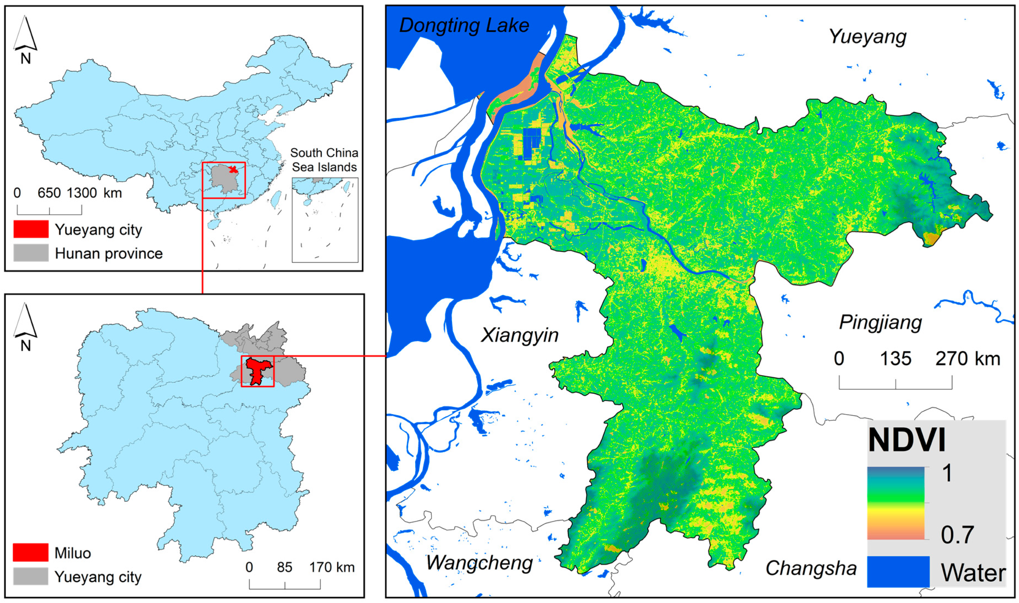
2.1. Study Area

Miluo is a county-level city located on the lower reaches of the Miluo River in Hunan Province, China. It is bounded by Dongting Lake to the west, Pingjiang County to the east, Changsha County, and Wangcheng District in Changsha City to the south, and Xiangyin County and Yuanjiang City to the west (Figure 1) [24] As an important ecological barrier for Dongting Lake, the Miluo River National Wetland Park covers an area of 2954.1 hectares. Miluo is situated in a subtropical monsoon climate zone, characterized by four distinct seasons, abundant heat, and concentrated rainfall. It receives a total annual precipitation of 1345.4 mm and has an average annual temperature of 17 °C [25]. The favorable combination of light, heat, and water makes Miluo an ideal location for the growth and maturation of double-season rice and subtropical economic forestry, providing a favorable climatic environment for agricultural production [26]. Miluo has a resident population of over 630,000, according to the 7th Chinese census [27]. The city’s agricultural economy is well established, producing a wide range of high-quality agricultural products and high yield, and is designated as a national base county for commercial grain production.

2.2. Datasets

The present study utilized various types of data, including Landsat remote sensing satellite imagery [28], the Harmonized world soil database (HWSD) [29], temperature data [30], precipitation data [30], normalized difference vegetation index (NDVI) data, elevation data, and Terraclimate reanalysis data [31]. The data preprocessing process entailed converting all spatial data to the WGS 1984 coordinate system and aggregating monthly data to annual data. For Landsat image data, declouding was performed using the CFMASK model [32]; stitching and median synthesis were conducted for summer data, and Google Earth Engine [33] was utilized to process the data. To obtain the Miluo land use/cover change (LUCC) data, a random forest model was used to calculate the data, with 10,734 sample points of different feature types collected each year, based on Google historical imagery, and an average overall accuracy of >95%. Supplementary Table S1 provides more detailed information about the study data.

2.3. Methods

The methodological approach for this study is presented in Figure 2 and consists of three main parts. Firstly, we employed the Google Earth Engine (GEE) platform to integrate all available Landsat image data for Miluo across each year (June, July, and August). These images were then processed through declouding, equalization, and median synthesis techniques to generate annual synthetic image data. Taking into consideration previous studies and the unique characteristics of the study area, we selected a suitable set of variables and utilized a random forest model to map Miluo’s LUCC at five-year intervals from 2000 to 2020. Secondly, we employed multiple models, including InVEST, CASA, and RUSLE, in conjunction with multi-source data (see Supplementary Text S1) to quantify Miluo’s ecosystem services (water retention, habitat quality, soil retention, food production, carbon retention, and climate regulation) over the past two decades. Finally, we conducted correlation analysis to examine the trade-offs and synergistic relationships among Miluo’s ecosystem services at both the pixel and county levels. Additionally, we investigated the drivers of Miluo’s ecosystem services, such as human activities and natural factors, using reanalysis data and multi-source remote sensing data. The study data can be found in Supplementary Table S1.

2.3.1. Land Use/Cover Change (LUCC) Classification

This study used a random forest (RF) model for land use classification, which is an integrated learning algorithm based on the formation of multiple decision trees and is widely used in ES research. Compared to other classification models, RF has several significant advantages. Not only does it perform well when dealing with outliers and noise, but also when dealing with multidimensional data, and the higher accuracy of the classification is also a unique advantage of the RF model [34,35]. In addition, recent studies have shown that the RF model was the most popular classifier among the many GEE-based studies in the past decade [36], and therefore, we chose RF as the classification model for LUCC in this study. Based on Google Earth and Planet Lab, we collected a sample set of 10,734 features using visual interpretation, of which we set 80% as training samples and the other 20% as validation samples. Twelve variables were selected as feature variables in the RF model. The 12 feature variables were blue band (Blue), green band (Green), red band (Red), near infrared band (NIR), shortwave infrared 1 band (SWIR1), shortwave infrared 2 band (SWIR2), NDVI [37], normalized difference building index (NDBI) [38], normalized difference water index (NDWI) [39], modified normalized difference water index (MNDWI) [40], elevation (ELE), and slope (SLO).

2.3.2. Optimal Granularity of Ecosystem Type

Previous research has shown that ESs are spatially granularity-dependent [41,42], so determining the optimal granularity is crucial for ES-based policy options research [43]. The sensitivity of landscape pattern indices to different granularities is now commonly used by scholars to determine the optimal scale for ESs [44]. One of the more commonly used indicators is the coefficient of variation (CV) [45,46], which is a relative indicator used to quantify the dispersion of multidimensional data. The higher the CV of a landscape pattern index, the more sensitive that landscape pattern index is to spatial granularities. Then, by plotting the trend of the sensitive landscape pattern index against spatial granularities, the abrupt change point of the trend line of each landscape pattern index change is extracted, which is the optimal granularity for that index.
In view of the actual spatial extent characteristics of Miluo and previous studies [47], this study calculated the CV of different landscape pattern indices in the range of 30 m–300 m at an interval of 10 m. We selected 17 representative landscape pattern indices in terms of the shape index, aggregation index, diversity index, and edge index. All landscape pattern indices were calculated in Fragstats software. For more information about them, please see Supplementary Table S1.

2.3.3. Quantification of Trade-Offs/Synergies between ESs

This study analyzed the trade-offs and synergistic relationships between Miluo ESs using statistical methods based on pixel and country scales. Spearman correlation coefficients [48] were used to quantify the degree of correlation between ESs at the 0.05 level, and when the correlation coefficient between the two was negative, this indicated that the ES pair had a trade-off relationship, and vice versa for a synergistic relationship.
R m n = i = 1 x ( m i m ) ( n i n ) i = 1 x ( m i m ) 2 i = 1 x ( n i n ) 2
where Rmn is the correlation coefficient between m and n variables, mi and ni are the ESs for year i, x is the year, and x is 5 in this paper.

2.3.4. Mann-Kendall Test

The Mann-Kendall test was used to test the significance of trends in changes in ESs:
s g n ( X j X i ) = + 1 i f   ( X j X i ) > 0   0 i f   ( X j X i ) = 0 1 i f   ( X j X i ) < 0  
V a r ( S ) = 1 18 n ( n 1 ) ( 2 n + 5 ) p = 1 q t p ( t p 1 ) ( 2 t p + 5 )
Z M K = S 1 V a r ( S ) i f   S > 0 0 i f   S = 0 S + 1 V a r ( S ) i f   S < 0
where n is 5, and the value of ZMK is within (−∞, +∞). At a given significance level α, when |ZMK| > Z1−α/2, the changing trend is significant in the time series at the 0.05 level.

3. Results

3.1. Optimal Granularity

Table 1 shows the CV of each landscape pattern index for Miluo from 2000 to 2020. As seen from the Table 1, the sum of all landscape pattern indices is the largest in 2020. In addition, indicators with higher CV values are more sensitive to spatial granularity, and with reference to previous studies [47], landscape pattern indices with CVs greater than 10% were identified as sensitive indicators. Therefore, this study plots the trends of NP, PD, LPI, ED, LSI, PLADJ, SPLIT, and AI with spatial granularity in 2020 (Figure 3).
Figure 3 shows that the change of LSI, PD, ED, NP, AI, and PLADJ generally showed a decreasing trend. Among them, LSI, PD, ED, and NP did not show abrupt change points, while the abrupt change points of AI and PLADJ both appeared at 180 m. In addition, SPLIT and LPI showed fluctuating change trends in general, and abrupt change points appeared at 40 m and 50 m, respectively. Therefore, to satisfy all landscape pattern index rules, we finally used 40 m as the best granularity for Miluo’s ESs from 2000 to 2020.

3.2. Ecosystem Pattern (LUCC)

We collected land survey samples from Miluo for five years and mapped Miluo’s ecosystem distribution pattern based on the RF model. Figure 4 and Supplementary Tables S3–S5 show the results of the accuracy validation of the LUCC data in this study. From Figure 4a and Supplementary Table S3, it can be seen that the user accuracies for all ecosystem types were higher than 0.8, and most of them exceeded 0.9 during 2000–2020. On the other hand, Figure 4c and Supplementary Table S4 show that the producer accuracy for most ecosystem types was higher than 0.8, with the highest user accuracy for the cropland and the lowest user accuracy for the grassland. In addition, the overall accuracy and kappa for all five years were above 0.9. These results indicate that the LUCC data produced in this study have high precision and can be accurately applied to the study of ESs in Miluo.
In the past two decades, Miluo’s ecosystem type has been dominated by cropland and forest. In 2020, the areas of cropland and forest were 716.15 km2 and 525.15 km2, respectively, and the area percentages were 42.93% and 31.48%, respectively, for a total of 74.41%. For spatial distribution, cropland was mainly distributed in the northwest. In contrast, forest was mainly distributed in the mountainous areas in the northeast and south. Among all the ecosystem types, the areas of garden, bareland, and wetland were the smallest, with values of 44.18 km2, 18.93 km2, and 20.89 km2, respectively, and the total proportion of their area was only 5.03%. The water was mainly located in Dongting Lake in northeastern Miluo, which, as shown in Figure 5, has shown an upwards trend in the last 20 years, directly due to the gradual conversion of wetlands to water (Figure 6), which was probably due to the influence of variables such as precipitation, surface runoff, and evapotranspiration that have changed the water balance in the region. From 2000 to 2020, forest and wetland mostly decreased, with decreases of 78.74 km2 and 28.26 km2, respectively. In addition, the area of built-up land showed a rapid growth trend, with an increase of 117.56 km2, and as shown in Figure 6, the expansion of built-up land was mainly through encroachment on cropland.

3.3. Distribution Patterns and Change in ESs

Referring to the method of Supplementary Text S1, we estimated the water retention (WR), habitat quality (HQ), soil retention (SR), food production (FP), carbon retention (CR), and climate regulation (CE) of Miluo City from 2000 to 2020 (Figure 7a). It can be seen from Figure 7 that although the ESs function has significant spatial heterogeneity, it generally presents a stable state in the time dimension. In addition, there was a strong spatial consistency between different ES pairs. CR, SR, WR, and HQ all showed the characteristics of high values located in mountainous areas and low values located in urban areas. In contrast, the spatial distribution of FP showed obvious differences. The high-value areas of FP were mainly located in cropland (northwest of Miluo), while the low-value areas were located in the northeast and southern mountainous areas, which are high-value areas of other ES. Overall, all five categories of ESs, with the exception of food production, show high values for forest. In contrast, the high-value areas of FP were mainly located in the central and northwestern regions. Miluo’s CE function increased by 50.45% from 2000 to 2020, with a rapid upwards trend of 261.46% between 2010 and 2020. CR services have risen by 4.36% in the last 20 years. FP increased by 9.23%, while WR, SR, and HQ all showed declines of −4.03%, −1.58%, and −9.12%, respectively. Although the ESs function of Miluo showed an overall downwards trend, the change range was small.

3.4. Tradeoffs and Synergies of ESs

Based on the pixel scale, we quantified the trade-offs and synergistic relationships for Miluo’s six ESs using the Spearman coefficient (Figure 8), resulting in a total of 15 trade-offs and synergistic effects. Among them, there were 10 synergistic relationships and five trade-off relationships. Fourteen of these 15 relationships passed the significance test (p < 0.05) and were statistically significant. Of all the relationships, the strongest synergy was WR-HQ, while the strongest trade-off was FP-HQ. The FP-related ES pairs all showed trade-offs, while other ES pairs were synergistic, suggesting that the rise in Miluo’s FP function over the last 20 years has led to a decline in other ES functions. For example, the heavy use of pesticides or fertilizers in agricultural production to increase FP often leads to problems such as biodiversity loss and water pollution [49]. Second, large amounts of agricultural irrigation not only affect surface runoff, but also reduce the WR of the land [50].
Figure 8 shows that in the static dimension, FP presented a trade-off with other ESs, i.e., there was an either/or relationship in terms of their spatial distribution [51]. In fact, ES trade-offs and synergies tend to exhibit a certain gradient effect due to differences in topography and climatic conditions [52]. This means that there is a clear pattern of spatial variation in ES and trade-offs/synergies. The gradient response of ES trade-offs and synergies to different drivers has still not been effectively explored. The results of regional-scale studies are, therefore, still somewhat flawed in terms of the fine-grained management of ecosystems. Here, we used the natural breakpoint method [53] to classify Miluo’s altitude, precipitation, and temperature into five categories, and analysed the ES trade-off/synergy relationship on the environmental factor gradient effect. To further elaborate the rationality of the gradient classification, we plotted the variation in precipitation and temperature composition with altitude gradient (Figure 9d), which shows that there are very large differences in precipitation and temperature composition on different altitude gradients, and the distribution of temperature and precipitation on different altitude gradients is regularly consistent with the results of the natural breakpoint method.
In the altitude gradient effect (Figure 9a), the WR, CR, CE, HQ, and SR functions gradually increased with increasing altitude, while FP showed a decreasing trend. Consistent with the results in Figure 8, FP showed a trade-off relationship with all other ESs, indicating that the higher the elevation, the weaker the FP function and the stronger the other ES. This is because the higher the altitude is, the steeper the terrain, the higher the precipitation, and the lower the temperature (Figure 9d). These factors may not only increase the difficulty of farmers’ farming practices, but also exacerbate the climatic risks of agricultural production [54]. Conversely, the higher the altitude, the less human activity there is, and the lower the potential ecological risk. In addition, the abundant precipitation brought by high altitude promotes the growth of vegetation, which not only enhances the vegetation’s carbon sequestration capacity, but also consolidates the soil’s water and soil conservation function [55]. Similarly, in the gradient effect of the precipitation factor (Figure 9b), ES showed a positive effect, except for FP. There was a trade-off relationship between FP and all other ESs. Finally, in the temperature factor gradient effect (Figure 9c), only FP showed an increasing trend with increasing temperature, while all other ESs showed a decreasing trend. Higher temperatures can effectively increase the phenological period of crops, resulting in higher food production [56]. On the other hand, higher temperatures increase the transpiration and respiration of vegetation water, leading to a decrease in surface water and soil water content, and an increase in carbon production from the heterotrophic respiration of vegetation [57].
Figure 10 shows a pixel-scale map of Miluo’s 15 ES trade-off/synergy relationships and area during 2000–2020. As shown in Figure 10, at the pixel scale (time dimension), FP showed a trade-off with CR, WR, HQ, and SR. In addition, SR showed trade-offs with most ES functions (except WR). This is inconsistent with the results of the trade-off/synergy analysis for the static dimension (Figure 8). This suggests that there was no uniformity in the trade-off/synergistic relationship between ES functions in Miluo under static and dynamic dimensions. This is because, under the static dimension, LUCC is the dominant factor driving the spatial distribution of ES [58]. In contrast, under the dynamics dimension, interactions between ESs are driven more by physical processes involving energy exchange and material cycling between vegetation, hydrology, and meteorology [59]. In the case of SR, for example, in the static dimension, the areas of high SR values were mainly located in forest (Figure 7), and the areas of high CR service values were also located in forest areas. In contrast, under the dynamic dimension, SR was the more stable ES [60], showing a slight downwards trend over the past 20 years (Figure 7), while CR was mainly influenced by the growth state of vegetation, showing a more substantial strengthening trend, probably due to the lagging changes in vegetation influenced by climatic factors (temperature, rainfall, etc.) [61]. The same phenomenon also occurred between HQ and WR. Unlike the pixel-scale results, synergy between ESs at the country scale is dominant (Figure 11). Only a trade-off relationship was shown between SR and WR. (Figure 11b). The relationship between the eight ES pairs was optimized (trade-off to synergistic relationship) compared to the results at the pixel scale.

3.5. Drive Analysis

This study explored the time series drivers of Miluo’s ESs based on multiple linear regression using multi-source remote sensing datasets with TerraClimate reanalysis data. Eleven variable indicators were selected for evaluation, including precipitation (PRE), soil moisture (SOIL), actual evapotranspiration (AET), climate water deficit (DEF), air temperature (TEMP), surface runoff (SR), potential evapotranspiration (PET), actual evapotranspiration (AET), population density (POP), electricity consumption (EC), and carbon emissions (CM). Figure 12 shows the ranking of the temporal drivers (in descending order) for CE, CR, FP, HQ, SR, and WR. Human activities play a dominant role in the temporal variation in all ESs, with CE, FP, and WR being dominated by population density, and CR and HQ being dominated by EC. In terms of natural factors, surface runoff and soil moisture are the main drivers; for example, the dominant factor for SR was soil moisture. Second, PDSI, AET, PET, and DEF had less influence on Miluo’s ESs. Our analysis suggests that the nexus effect of human activities and natural factors (climate change) has a broad impact on Miluo’s ESs.
Based on the findings of this study, we propose the following recommendations. In the future, the region’s pursuit of multiple development goals will attract a diverse range of stakeholders with varying development aspirations. Consequently, the inherent conflict between development goals and conservation will persist. To align with international benchmarks in terms of ecological and environmental quality, it is crucial to address the challenges associated with construction land and make decisions considering ESs perspectives. This approach will enhance the synergy between conservation and development. In areas with high ES values, the continued strict implementation of ecological mitigation and protection policies is essential. In urban land use areas, it is imperative to adopt scientifically informed and rational urban planning strategies based on the concept of smart growth. This entails maximizing the efficiency of urban land use to curb the rapid expansion of urban areas, while vigorously fostering the development of new industries and reducing resource consumption. Furthermore, strict control over the allocation of land for construction is necessary. It is important to reasonably allocate ecological land to build a green ecological pattern that promotes harmony and unity between the ecological environment and human activities.

3.6. Exposure Analysis

We investigated the relationship between ESs trends and changes in CM, EC, and POP during this period at the county scale and the pixel scale. In 27 counties, the ESs trend was greater than zero. The highest ESs trend was found in Fan-SFQ (14.01 × 10⁻³), which was composed of four villages and is a tea demonstration farm in Miluo. It was followed by Huangshi (12.11 × 10⁻³) and Dajing (10.41 × 10⁻³). In the past 20 years, those counties exposed to the increasing trend of ESs increased a total of 59 × 103 tons of CM (Figure 13b), 260 × 106 Kwh of EC (Figure 13a), and 53 × 103 of POP (Figure 13c). The 10 counties exposed to a decreasing trend in ESs increased by 59 × 103 tons of CM (Figure 13b), 300 × 106 Kwh of EC (Figure 13a), and 50 × 103 of POP (Figure 13c).
In 2020, there was a strong linear relationship between CM, EC and POP at the county scale (Figure 13d,e). However, the ESs trend varied greatly among counties. Xinshi’s ESs trend over the past 20 years reached −11.35 × 10⁻³, ranking third from the bottom among all counties. in 2020, Xinshi consumed 69.46 × 10⁶ Kwh of EC (Figure 13b), accounting for 8.13% of Miluo’s total EC, and produced 30.39 × 10³ tons of CM (Figure 13a), which contributed 9.16% to Miluo’s total CM, indicating that Xinshi was in a rapid development stage and may face significant challenges to the ecological environment. In addition, as the main urban area of Miluo, the ESs trends of Chengjiao and Chengguan were −7.53 × 10⁻³ and −11.35 × 10⁻³, respectively. In 2020, their POP, EC, and CM accounted for 10.45%, 21.20%, and 14.11% of Miluo’s total, respectively. Then, in 2020, we investigated the exposure of CM, EC, and POP to ESs trends under static conditions. The increasing ESs trend affected one-half of the total CM (48.07%) (Figure 13f), total EC (48.33%) (Figure 13g), and total POP (52.47%) (Figure 13h). In addition, pixels exposed to the ESs decreasing trend had higher mean CM (Figure 13g), EC (Figure 13f), and POP (Figure 13h) than those exposed to the ESs increasing trend. Therefore, according to the environmental Kuznets hypothesis [62], Miluo’s urbanization was still in a rapid development stage in the past 20 years and has a long way to go before mature urbanization.

4. Discussion

This study investigated the trade-off and synergistic mechanisms of ESs in wetland city, using Miluo, China as an example, and based on multiple ecophysical process models. Unlike previous studies, this research adopted a multi-scale perspective. Firstly, we generated the most accurate high-resolution land-use dataset available for Miluo, by utilizing a random forest algorithm and a large collection of measured sample datasets. Furthermore, we observed a clear synergistic relationship among ESs in Miluo over the past 20 years, at both the pixel and county scales. However, we also identify a trade-off relationship between food production (FP) and other ESs. Moreover, this relationship holds true for elevation, precipitation, and temperature gradients.

4.1. ESs Accuracy Verification

The accuracy of ESs has important implications for study results. Here, we selected WR, CR and HQ for accuracy validation, considering the availability of validation data. First, we used human footprint data [63] to validate the accuracy of HQ. Human activities are the main cause of HQ degradation, so there is a negative correlation between human footprint and HQ. We fitted the correlation between HQ and human footprint based at the county scale (Figure 14a). Then, we verified the accuracy of WR using the MNDWI (Figure 14a). Finally, we verified the accuracy of CR using the NPP product of MOD17A3 [64] (Figure 14c). As can be seen from Figure 14, the HQ, WR and CR simulated in this study can reflect the major ecosystem services of Miluo well.

4.2. Limitations and Priorities for Future Work

The significance of remote sensing data in ES research has been widely acknowledged; however, the uncertainty between different sources of the same indicator data is still unclear. Furthermore, the application of machine learning-based land use and land cover (LUCC) classification introduces a certain level of uncertainty to the study, as it inherently entails the presence of classification errors. This study used CM, POP, and EC as the main indicators of human activities, which is inadequate in future studies. We will comprehensively expand the connotation of human activities in the future. In addition, the driving mechanisms and relationships between natural factors and human activities on ESs need to be further explored. Finally, constrained by the limited validation data, we did not validate the accuracy of the simulated CE, SR, and FP. We believe that future collaborative research with geographers and ecologists will effectively address these limitations and facilitate dynamic monitoring and precise control of ESs in practice.

4.3. Policy Recommendations

The analysis of ESs trade-offs/synergies and their drivers reflects the basic ecosystem local conditions for Miluo. The conclusions drawn from this study suggest that strict control measures should be implemented in the nature reserve areas such as wetlands and lakes, and that any production and business activities should be strictly prohibited in the area. In addition the natural ecological landscape should be maintained and the restoration of the ecologically fragmented surface of the rivers in the Dongting Lake area and Miluo River area should be strengthened to protect the ecological security of the upstream water source of the Miluo River in Bai Sugar Town. In addition, the forest area is also a key area for ecological control. For this region, a graded protection and specific management approach for forest land should be implemented, and a compensation mechanism for forest land protection should be formed and improved. As for the arable land area, it should develop efficient agriculture, carry out the construction of high-standard basic farmland and intensify farmland. Urban areas should pay attention to the harmonious development of man and nature, strengthen the management of urban vegetation for human enhancement, and promote the construction of urban environment.

5. Conclusions

In the context of increased human activity and global climate change, understanding the changes in Miluo’s ESs is crucial for maintaining biodiversity stability and ecosystem balance in the Dongting Lake Basin. Therefore, we utilized multi-source data to estimate Miluo’s major ESs (water retention, habitat quality, soil retention, food production, carbon retention, and climate regulation) from 2000 to 2020 using multiple ES assessment models. We analyzed the spatiotemporal variability of Miluo’s ESs over the past 20 years and explored the trade-offs and synergies between ESs at both the pixel scale and county scale.
The findings revealed several key points. Firstly, arable land dominated Miluo’s ecosystem type, covering 42.93% of the city’s total area. Urban expansion, particularly the conversion of farmland and forest, was the most significant change observed in the past two decades, while other ecosystem types remained relatively stable. Secondly, woodlands exhibited the highest levels of ESs over the studied period. However, all six ESs experienced varying degrees of decline, with urban ESs showing a sharp decrease.
In terms of the static dimension dominated by land use and land cover (LUCC) data, food production (FP) demonstrated trade-offs with other ESs, whereas the remaining ESs exhibited synergistic relationships with each other. Notably, in the dynamic dimension at the pixel scale, soil retention (SR) displayed trade-offs with most ES functions, except for water retention (WR). At the county scale, eight pairs of ESs exhibited optimized relationships, transitioning from trade-offs to synergistic relationships. Finally, human activities emerged as the dominant factor driving the changes in Miluo’s ESs over the past 20 years.

Supplementary Materials

The following supporting information can be downloaded at: https://www.mdpi.com/article/10.3390/rs15143479/s1, Text S1: Ecosystem service estimates; Figure S1: Importance of feature variables based on RF model in Miluo during 2000–2020; Figure S2: Distribution maps LUCC classification sample in Miluo during 2000–2020; Table S1: Detailed description of the data. Table S2: Details of the 17 landscape pattern indices; Table S3: User accuracy of LUCC data; Table S4: Producer accuracy of LUCC data. Table S5: Overall accuracy and Kappa of LUCC data; Table S6: Ecosystem mean runoff coefficient. 22 references [65,66,67,68,69,70,71,72,73,74,75,76,77,78,79,80,81,82,83,84,85,86] are included in the Supplementary Materials.

Author Contributions

Conceptualization, S.C.; Funding acquisition, X.H.; Investigation, S.C.; Methodology, D.X.; Project administration, X.H.; Resources, Y.W.; Software, C.C.; Validation, S.C.; Writing—original draft, S.C.; Writing—review & editing, T.B. All authors have read and agreed to the published version of the manuscript.

Funding

This research was funded by the Key Disciplines of State Forestry Administration of China (Grant No. 21 of Forest Ren Fa, 2016), Hunan Province “Double First-class” Cultivation discipline of China (No. 469 of Xiang Jiao Tong, 2018), Subjects of the Hunan Provincial Social Science Assessment Committee (Grant XSP21YBC408), and the Key Laboratory of Environmental Change and Natural Disaster of Ministry of Education, Beijing Normal University (Grant No. 2022-KF-13).

Data Availability Statement

Not applicable.

Acknowledgments

This work was partly supported by the Key Disciplines of State Forestry Administration of China (Grant No. 21 of Forest Ren Fa, 2016), Hunan Province “Double First-class” Cultivation discipline of China (No. 469 of Xiang Jiao Tong, 2018), Subjects of the Hunan Provincial Social Science Assessment Committee (Grant XSP21YBC408), and the Key Laboratory of Environmental Change and Natural Disaster of Ministry of Education, Beijing Normal University (Grant No. 2022-KF-13).

Conflicts of Interest

The authors declare no conflict of interest.

References

  1. Bennett, E.M.; Peterson, G.D.; Gordon, L.J. Understanding relationships among multiple ecosystem services. Ecol. Lett. 2009, 12, 1394–1404. [Google Scholar] [CrossRef] [PubMed]
  2. Daily, G.C.; Matson, P.A. Ecosystem services: From theory to implementation. Proc. Natl. Acad. Sci. USA 2008, 105, 9455–9456. [Google Scholar] [CrossRef]
  3. Uddin, M.S.; van Steveninck, E.R.; Stuip, M.; Shah, M.A.R. Economic valuation of provisioning and cultural services of a protected mangrove ecosystem: A case study on Sundarbans Reserve Forest, Bangladesh. Ecosyst. Serv. 2013, 5, 88–93. [Google Scholar] [CrossRef]
  4. Ernstson, H. The social production of ecosystem services: A framework for studying environmental justice and ecological complexity in urbanized landscapes. Landsc. Urban Plan. 2013, 109, 7–17. [Google Scholar] [CrossRef] [Green Version]
  5. Haase, D.; Schwarz, N.; Strohbach, M.; Kroll, F.; Seppelt, R. Synergies, trade-offs, and losses of ecosystem services in urban regions: An integrated multiscale framework applied to the Leipzig-Halle Region, Germany. Ecol. Soc. 2012, 17, 22. [Google Scholar] [CrossRef] [Green Version]
  6. Bennett, E.M.; Cramer, W.; Begossi, A.; Cundill, G.; Diaz, S.; Egoh, B.N.; Geijzendorffer, I.R.; Krug, C.B.; Lavorel, S.; Lazos, E.; et al. Linking biodiversity, ecosystem services, and human well-being: Three challenges for designing research for sustainability. Curr. Opin. Environ. Sustain. 2015, 14, 76–85. [Google Scholar] [CrossRef]
  7. Feng, Z.; Jin, X.; Chen, T.; Wu, J. Understanding trade-offs and synergies of ecosystem services to support the decision-making in the Beijing–Tianjin–Hebei region. Land Use Policy 2021, 106, 105446. [Google Scholar] [CrossRef]
  8. Liu, H.; Zheng, L.; Wu, J.; Liao, Y.H. Past and future ecosystem service trade-offs in Poyang Lake Basin under different land use policy scenarios. Arab. J. Geosci. 2020, 13, 46. [Google Scholar] [CrossRef] [Green Version]
  9. Xu, D.; Yang, F.; Yu, L.; Zhou, Y.; Li, H.; Ma, J.; Huang, J.; Wei, J.; Xu, Y.; Zhang, C.; et al. Quantization of the coupling mechanism between eco-environmental quality and urbanization from multisource remote sensing data. J. Clean. Prod. 2021, 321, 128948. [Google Scholar] [CrossRef]
  10. Xu, D.; Cheng, J.; Xu, S.; Geng, J.; Yang, F.; Fang, H.; Xu, J.; Wang, S.; Wang, Y.; Huang, J.; et al. Understanding the Relationship between China’s Eco-Environmental Quality and Urbanization Using Multisource Remote Sensing Data. Remote Sens. 2022, 14, 198. [Google Scholar] [CrossRef]
  11. Zhai, T.; Zhang, D.; Zhao, C. How to optimize ecological compensation to alleviate environmental injustice in different cities in the Yellow River Basin? A case of integrating ecosystem service supply, demand and flow. Sustain. Cities Soc. 2021, 75, 103341. [Google Scholar] [CrossRef]
  12. Gonzalez, A.; Germain, R.M.; Srivastava, D.S.; Filotas, E.; Dee, L.E.; Gravel, D.; Thompson, P.L.; Isbell, F.; Wang, S.P.; Kefi, S.; et al. Scaling-up biodiversity-ecosystem functioning research. Ecol. Lett. 2020, 23, 757–776. [Google Scholar] [CrossRef] [PubMed] [Green Version]
  13. Milder, J.C.; Hart, A.K.; Dobie, P.; Minai, J.; Zaleski, C. Integrated landscape initiatives for African agriculture, development, and conservation: A region-wide assessment. World Dev. 2014, 54, 68–80. [Google Scholar] [CrossRef]
  14. Zhang, J.; Guo, W.; Cheng, C.; Minai, J.; Zaleski, C. Trade-offs and driving factors of multiple ecosystem services and bundles under spatiotemporal changes in the Danjiangkou Basin, China. Ecol. Indic. 2022, 144, 109550. [Google Scholar] [CrossRef]
  15. Cord, A.F.; Bartkowski, B.; Beckmann, M.; Dittrich, A.; Hermans-Neumann, K.; Kaim, A.; Lienhoop, N.; Locher-Krause, K.; Priess, J.; Schroter-Schlaack, C.; et al. Towards systematic analyses of ecosystem service trade-offs and synergies: Main concepts, methods and the road ahead. Ecosyst. Serv. 2017, 28, 264–272. [Google Scholar] [CrossRef]
  16. Yang, M.; Gao, X.; Zhao, X.; Wu, P. Scale effect and spatially explicit drivers of interactions between ecosystem services—A case study from the Loess Plateau. Sci. Total Environ. 2021, 785, 147389. [Google Scholar] [CrossRef]
  17. Howe, C.; Suich, H.; Vira, B.; Mace, G.M. Creating win–wins from trade-offs? Ecosystem services for human well-being: A meta-analysis of ecosystem service trade-offs and synergies in the real world. Glob. Environ. Change 2014, 28, 263–275. [Google Scholar] [CrossRef] [Green Version]
  18. Yuan, B.; Fu, L.; Zou, Y.; Zhang, S.; Chen, X.; Li, F.; Deng, Z.; Xie, Y. Spatiotemporal change detection of ecological quality and the associated affecting factors in Dongting Lake Basin based on RSEI. J. Clean. Prod. 2021, 302, 126995. [Google Scholar] [CrossRef]
  19. Jiang, X.; Ma, R.; Ma, T.; Sun, Z. Modelling the effects of water diversion projects on surface water and groundwater interactions in the central Yangtze River basin. Sci. Total Environ. 2022, 830, 154606. [Google Scholar] [CrossRef]
  20. Chen, J.X.; Zhang, Y.; Zheng, S. Ecoefficiency, environmental regulation opportunity costs, and interregional industrial transfers: Evidence from the Yangtze River Economic Belt in China. J. Clean. Prod. 2019, 233, 611–625. [Google Scholar] [CrossRef]
  21. Lai, Z.; Chen, M.; Liu, T. Changes in and prospects for cultivated land use since the reform and opening up in China. Land Use Policy 2020, 97, 104781. [Google Scholar] [CrossRef]
  22. Gao, Y. Yangzi Waters: Transforming the Water Regime of the Jianghan Plain in Late Imperial China; Brill: Leiden, The Netherlands, 2022. [Google Scholar]
  23. Xu, X.; Su, Y.; Shao, H.; Huang, S.; Liu, G. Evaluation of symbiotic of waste resources ecosystem: A case study of Hunan Miluo Recycling Economy Industrial Park in China. Environ. Dev. Sustain. 2022, 25, 1131–1150. [Google Scholar] [CrossRef]
  24. Wang, C.; Lu, F.; Sun, Q.; Zuo, L.; Geng, H. How do policies take effect in the development of the urban mining industry? A local capability perspective: Evidence from Miluo, China (2000–2017). J. Clean. Prod. 2019, 240, 118216. [Google Scholar] [CrossRef]
  25. Xiao, K.Q.; Dong, H.G.; Guo, J.; Li, Y.; Chen, B. Study on Spatial Variability of Farmland Soil Nutrients in Miluo City, Hunan Province. South China Geol. 2021, 37, 369–376. [Google Scholar]
  26. Liang, J.Y.; Chien, Y.H. Effects of feeding frequency and photoperiod on water quality and crop production in a tilapia–water spinach raft aquaponics system. Int. Biodeterior. Biodegrad. 2013, 85, 693–700. [Google Scholar] [CrossRef]
  27. Xu, H.; Zhou, H.; Xu, Y. Development of educational attainment and gender equality in China: New evidence from the 7th National Census. China Popul. Dev. Stud. 2022, 6, 425–451. [Google Scholar] [CrossRef]
  28. Irons, J.R.; Dwyer, J.L.; Barsi, J.A. The next Landsat satellite: The Landsat data continuity mission. Remote Sens. Environ. 2012, 122, 11–21. [Google Scholar] [CrossRef] [Green Version]
  29. Nachtergaele, F.; Velthuizen, H.V.; Verelst, L. Harmonized World Soil Database (HWSD); Food and Agriculture Organization of the United Nations: Rome, Italy, 2009. [Google Scholar]
  30. Peng, S.; Ding, Y.; Liu, W.; Li, Z. 1 km monthly temperature and precipitation dataset for China from 1901 to 2017. Earth Syst. Sci. Data 2019, 11, 1931–1946. [Google Scholar] [CrossRef] [Green Version]
  31. Abatzoglou, J.T.; Dobrowski, S.Z.; Parks, S.A.; Hegewisch, K.C. TerraClimate, a high-resolution global dataset of monthly climate and climatic water balance from 1958–2015. Sci. Data 2018, 5, 170191. [Google Scholar] [CrossRef] [Green Version]
  32. Foga, S.; Scaramuzza, P.L.; Guo, S.; Zhu, Z.; Dilley, R.D.; Beckmann, T.; Schmidt, G.L.; Dwyer, J.L.; Hughes, M.J.; Laue, B. Cloud detection algorithm comparison and validation for operational Landsat data products. Remote Sens. Environ. 2017, 194, 379–390. [Google Scholar] [CrossRef] [Green Version]
  33. Gorelick, N.; Hancher, M.; Dixon, M.; Ilyushchenko, S.; Moore, R. Google Earth Engine: Planetary-scale geospatial analysis for everyone. Remote Sens. Environ. 2017, 202, 18–27. [Google Scholar] [CrossRef]
  34. Rodriguez-Galiano, V.F.; Chica-Rivas, M. Evaluation of different machine learning methods for land cover mapping of a Mediterranean area using multiseasonal Landsat images and Digital Terrain Models. Int. J. Digit. Earth 2014, 7, 492–509. [Google Scholar] [CrossRef]
  35. Abdel-Rahman, E.M.; Mutanga, O.; Adam, E.; Ismail, R. Detecting Sirex noctilio grey-attacked and lightning-struck pine trees using airborne hyperspectral data, random forest and support vector machines classifiers. ISPRS J. Photogramm. Remote Sens. 2014, 88, 48–59. [Google Scholar] [CrossRef]
  36. Tamiminia, H.; Salehi, B.; Mahdianpari, M.; Quackenbush, L.; Adeli, S.; Brisco, B. Google Earth Engine for geo-big data applications: A meta-analysis and systematic review. ISPRS J. Photogramm. Remote Sens. 2020, 164, 152–170. [Google Scholar] [CrossRef]
  37. Pettorelli, N. The Normalized Difference Vegetation Index; Oxford University Press: Oxford, UK, 2013. [Google Scholar]
  38. Zhao, H.; Chen, X. Use of normalized difference bareness index in quickly mapping bare areas from TM/ETM+. Int. Geosci. Remote Sens. Symp. 2005, 3, 1666. [Google Scholar]
  39. Gao, B.C. NDWI—A normalized difference water index for remote sensing of vegetation liquid water from space. Remote Sens. Environ. 1996, 58, 257–266. [Google Scholar] [CrossRef]
  40. Xu, H. Modification of normalized difference water index (NDWI) to enhance open water features in remotely sensed imagery. Int. J. Remote Sens. 2006, 27, 3025–3033. [Google Scholar] [CrossRef]
  41. Mayer, A.L.; Rietkerk, M. The dynamic regime concept for ecosystem management and restoration. BioScience 2004, 54, 1013–1020. [Google Scholar] [CrossRef] [Green Version]
  42. Fonseca, M.; Whitfield, P.E.; Kelly, N.M.; Bell, S.S. Modelling seagrass landscape pattern and associated ecological attributes. Ecol. Appl. 2002, 12, 218–237. [Google Scholar] [CrossRef]
  43. Briscoe, G.; Sadedin, S.; De Wilde, P. Digital ecosystems: Ecosystem-oriented architectures. Nat. Comput. 2011, 10, 1143–1194. [Google Scholar] [CrossRef] [Green Version]
  44. Guan, D.; Jiang, Y.; Cheng, L. How can the landscape ecological security pattern be quantitatively optimized and effectively evaluated? An integrated analysis with the granularity inverse method and landscape indicators. Environ. Sci. Pollut. Res. 2022, 29, 41590–41616. [Google Scholar] [CrossRef] [PubMed]
  45. Curto, J.D.; Pinto, J.C. The coefficient of variation asymptotic distribution in the case of noniid random variables. J. Appl. Stat. 2009, 36, 21–32. [Google Scholar] [CrossRef]
  46. Jalilibal, Z.; Amiri, A.; Castagliola, P.; Khoo, M. Monitoring the coefficient of variation: A literature review. Comput. Ind. Eng. 2021, 161, 107600. [Google Scholar] [CrossRef]
  47. Song, Y.; Zhang, Z.; Niu, B.; Li, X. Temporal and spatial patterns of landscape pattern vulnerability in the Yellow River Delta from 2005–2018. Soil Water Conserv. Bull. 2021, 41, 258–266. [Google Scholar] [CrossRef]
  48. Myers, L.; Sirois, M.J. Spearman correlation coefficients, differences between. Encycl. Stat. Sci. 2004, 12. [Google Scholar] [CrossRef]
  49. Ongley, E.D. Control of Water Pollution from Agriculture; Food & Agriculture Organization: Rome, Italy, 1996. [Google Scholar]
  50. Pimentel, D.; Houser, J.; Preiss, E.; White, O.; Fang, H.; Mesnick, L.; Barsky, T.; Tariche, S.; Schreck, J.; Alpert, S. Water resources: Agriculture, the environment, and society. BioScience 1997, 47, 97–106. [Google Scholar] [CrossRef] [Green Version]
  51. Teng, Y.; Zhan, J.; Liu, W.; Chu, X.; Zhang, F.; Wang, C.; Wang, L. Spatial heterogeneity of ecosystem services trade-offs among ecosystem service bundles in an alpine mountainous region: A case-study in the Qilian Mountains, Northwest China. Land Degrad. Dev. 2022, 33, 1846–1861. [Google Scholar] [CrossRef]
  52. Lin, S.; Wu, R.; Yang, F.; Wang, J.; Wu, W. Spatial trade-offs and synergies among ecosystem services within a global biodiversity hotspot. Ecol. Indic. 2018, 84, 371–381. [Google Scholar] [CrossRef]
  53. Xiao, W.; Lv, X.; Zhao, Y.; Sun, H.; Li, J. Ecological resilience assessment of an arid coal mining area using index of entropy and linear weighted analysis: A case study of Shendong Coalfield, China. Ecol. Indic. 2020, 109, 105843. [Google Scholar] [CrossRef]
  54. Uddin, M.N.; Bokelmann, W.; Entsminger, J.S. Factors affecting farmers’ adaptation strategies to environmental degradation and climate change effects: A farm level study in Bangladesh. Climate 2014, 2, 223–241. [Google Scholar] [CrossRef] [Green Version]
  55. Yang, W.; Min, Z.; Yang, M.; Yan, J. Exploration of the Implementation of Carbon Neutralization in the Field of Natural Resources under the Background of Sustainable Development—An Overview. Int. J. Environ. Res. Public Health 2022, 19, 14109. [Google Scholar] [CrossRef] [PubMed]
  56. Hatfield, J.L.; Prueger, J.H. Temperature extremes: Effect on plant growth and development. Weather. Clim. Extrem. 2015, 10, 4–10. [Google Scholar] [CrossRef] [Green Version]
  57. Cramer, W.; Bondeau, A.; Woodward, F.I.; Prentice, I.; Ramankutty, N. Global response of terrestrial ecosystem structure and function to CO2 and climate change: Results from six dynamic global vegetation models. Glob. Change Biol. 2001, 7, 357–373. [Google Scholar] [CrossRef] [Green Version]
  58. Zhou, R.; Lin, M.; Gong, J.; Wu, Z. Spatiotemporal heterogeneity influencing mechanism of ecosystem services in the Pearl River Delta from the perspective of, LUCC. J. Geogr. Sci. 2019, 29, 831–845. [Google Scholar] [CrossRef] [Green Version]
  59. Archer, S.R.; Predick, K.I. An ecosystem services perspective on brush management: Research priorities for competing land-use objectives. J. Ecol. 2014, 102, 1394–1407. [Google Scholar] [CrossRef] [Green Version]
  60. Palm, C.; Blanco-Canqui, H.; DeClerck, F.; Gatere, L.; Grace, P. Conservation agriculture and ecosystem services: An overview. Agric. Ecosyst. Environ. 2014, 187, 87–105. [Google Scholar] [CrossRef] [Green Version]
  61. Lal, R. Digging deeper: A holistic perspective of factors affecting soil organic carbon sequestration in agroecosystems. Glob. Change Biol. 2018, 24, 3285–3301. [Google Scholar] [CrossRef]
  62. Dinda, S. Environmental Kuznets curve hypothesis: A survey. Ecol. Econ. 2004, 49, 431–455. [Google Scholar] [CrossRef] [Green Version]
  63. Mu, H.; Li, X.; Wen, Y.; Huang, J.; Du, P.; Su, W.; Miao, S.; Geng, M. A global record of annual terrestrial Human Footprint dataset from 2000 to 2018. Sci. Data 2022, 9, 176. [Google Scholar] [CrossRef]
  64. Running, S.; Mu, Q.; Zhao, M. Mod17a3h Modis/Terra net Primary Production Yearly l4 Global 500 m sin grid v006. 2015, Distributed by Nasa Eosdis Land Processes Daac. Available online: https://lpdaac.usgs.gov/products/mod17a3hv006/ (accessed on 23 January 2023).
  65. Wilder, T.C.; Rheinhardt, R.D.; Noble, C.V. A Regional Guidebook for Applying the Hydrogeomorphic Approach to Assessing Wetland Functions of Forested Wetlands in Alluvial Valleys of the Coastal Plain of the Southeastern United States; Engineer Research and Development Center Vicksburg MS Environmental Lab: Vicksburg, MS, USA, 2013. [Google Scholar]
  66. Zeng, C.; Wanyu, Q.; Mao, Y.; Liu, R.; Yu, B.; Dong, X. Study on Water Conservation Ecological Service Function and Its Value Response Mechanism in Nested Area of Water Conservancy Project. Front. Environ. Sci. 2022, 720, 887040. [Google Scholar] [CrossRef]
  67. Nippgen, F.; McGlynn, B.L.; Emanuel, R.E.; Vose, J.M. Watershed memory at the Coweeta Hydrologic Laboratory: The effect of past precipitation and storage on hydrologic response. Water Resour. Res. 2016, 52, 1673–1695. [Google Scholar] [CrossRef] [Green Version]
  68. Xiao, Y.; Xiong, Q.L.; Liang, P.H.; Xiao, Q. Potential risk to water resources under eco-restoration policy and global change in the Tibetan Plateau. Environ. Res. Lett. 2021, 16, 094004. [Google Scholar] [CrossRef]
  69. Rao, E.; Xiao, Y.; Ouyang, Z.Y.; Zheng, H. Spatial characteristics of soil conservation service and its impact factors in Hainan Island. Acta Ecol. Sin. 2013, 33, 746–755. (In Chinese) [Google Scholar] [CrossRef] [Green Version]
  70. Ganasri, B.P.; Ramesh, H. Assessment of soil erosion by RUSLE model using remote sensing and GIS-A case study of Nethravathi Basin. Geosci. Front. 2016, 7, 953–961. [Google Scholar] [CrossRef] [Green Version]
  71. Renard, K.G.; Foster, G.R.; Weesies, G.A.; McCool, D.K.; YoDer, D.C. Predicting Soil Erosion by Water: A Guide to Conservation Planning with the Revised Universal Soil Loss Equation (RUSLE); Handbook No. 703; U.S. Department of Agriculture: Washington, DC, USA, 1997.
  72. Xiao, Y.; Xiao, Q.; Xiong, Q.; Yang, Z. Effects of ecological restoration measures on soil erosion risk in the Three Gorges Reservoir area since the 1980s. GeoHealth 2020, 4, e2020GH000274. [Google Scholar] [CrossRef]
  73. Fayas, C.M.; Abeysingha, N.S.; Nirmanee, K.G.S.; Samaratung, D.; Mallawatantri, A. Soil loss estimation using rusle model to prioritize erosion control in KELANI river basin in Sri Lanka. Int. Soil Water Conserv. Res. 2019, 7, 130–137. [Google Scholar] [CrossRef]
  74. Williams, J.R.; Renard, K.G.; Dyke, P.T. EPIC: A new method for assessing erosion’s effect on soil productivity. J. Soil Water Conserv. 1983, 38, 381–383. [Google Scholar]
  75. Xiao, Y.; Ouyang, Z.Y.; Xu, W.H.; Xiao, Y.; Zheng, H.; Xian, C.F. Optimizing hotspot areas for ecological planning and management based on biodiversity and ecosystem services. Chin. Geogr. Sci. 2016, 26, 256–269. [Google Scholar] [CrossRef] [Green Version]
  76. Law, B.E.; Waring, R.H.; Anthoni, P.M.; Aber, J.D. Measurements of gross and net ecosystem productivity and water vapour exchange of a Pinus ponderosa ecosystem, and an evaluation of two generalized models. Glob. Change Biol. 2000, 6, 155–168. [Google Scholar] [CrossRef]
  77. Bond-Lamberty, B.; Wang, C.; Gower, S.T. A global relationship between the heterotrophic and autotrophic components of soil respiration? Glob. Change Biol. 2004, 10, 1756–1766. [Google Scholar] [CrossRef]
  78. Wu, L.; Sun, C.; Fan, F. Estimating the characteristic spatiotemporal variation in habitat quality using the invest model—A case study from Guangdong-Hong Kong-Macao Greater Bay Area. Remote Sens. 2021, 13, 1008. [Google Scholar] [CrossRef]
  79. Gong, J.; Xie, Y.; Cao, E.; Huang, Q.; Li, H. Integration of InVEST-habitat quality model with landscape pattern indexes to assess mountain plant biodiversity change: A case study of Bailongjiang watershed in Gansu Province. J. Geogr. Sci. 2019, 29, 1193–1210. [Google Scholar] [CrossRef] [Green Version]
  80. Xia, H.; Yuan, S.; Prishchepov, A.V. Spatial-temporal heterogeneity of ecosystem service interactions and their social-ecological drivers: Implications for spatial planning and management. Resour. Conserv. Recycl. 2023, 189, 106767. [Google Scholar] [CrossRef]
  81. Chen, S.; Huang, Y.; Zou, J.; Shen, Q.; Hu, Z.; Qin, Y.; Chen, H.; Pan, G. Modeling interannual variability of global soil respiration from climate and soil properties. Agric. For. Meteorol. 2010, 150, 590–605. [Google Scholar] [CrossRef]
  82. Tardy, B.; Rivalland, V.; Huc, M.; Hagolle, O.; Marcq, S.; Boulet, G. A software tool for atmospheric correction and surface temperature estimation of Landsat infrared thermal data. Remote Sens. 2016, 8, 696. [Google Scholar] [CrossRef] [Green Version]
  83. Chen, J.; Gao, M.; Cheng, S.; Hou, W.; Song, M.; Liu, X.; Liu, Y. Global 1 km × 1 km gridded revised real gross domestic product and electricity consumption during 1992–2019 based on calibrated nighttime light data. Sci. Data 2022, 9, 202. [Google Scholar] [CrossRef]
  84. Tatem, A.J. WorldPop, open data for spatial demography. Sci. Data 2017, 4, 170004. [Google Scholar] [CrossRef]
  85. Oda, T.; Maksyutov, S.; Andres, R.J. The Open-source Data Inventory for Anthropogenic CO2, version 2016 (ODIAC2016): A global monthly fossil fuel CO2 gridded emissions data product for tracer transport simulations and surface flux inversions. Earth Syst. Sci. Data 2018, 10, 87–107. [Google Scholar] [CrossRef]
  86. Gong, S.; Xiao, Y.; Zheng, H.; Xiao, Y.; Ouyang, Z.Y. Spatial characteristics of water-conserving ecosystems in China and their influencing factors. J. Ecol. 2017, 37, 2455–2462. (In Chinese) [Google Scholar]
Figure 1. Study area. NDVI was from Landsat 8 for the summer of 2020. Water body data from Open Street Map (OSM).
Remotesensing 15 03479 g001
Figure 2. The method flow chart of this study. The six ESs include water retention (WR), habitat quality (HQ), soil retention (SR), food production (FP), carbon retention (CR), and climate regulation (CE). The methodological process comprised three primary components. Firstly, the land use and land cover change (LUCC) data of Miluo City spanning the period from 2000 to 2020 were extracted utilizing a random forest model. Subsequently, the ecological process model was employed to map the data pertaining to six ecosystem services in Miluo City over the past two decades. Lastly, an assessment was conducted to quantify the trade-offs and synergistic relationships between the six ecosystem services and their respective driving forces.
Remotesensing 15 03479 g002
Figure 3. Trends in sensitive landscape pattern indices with spatial granularity in Miluo during 2000–2020. The blue dashed line represents the spatial granularity at the point of the first abrupt change in the trend of the landscape pattern index. The granularity range in this study spans from 30 to 300 m, with a step size of 10 m.
Remotesensing 15 03479 g003
Figure 4. User accuracy (a), overall accuracy (b), producer accuracy (c) and kappa (d) of LUCC data in Miluo during 2000–2020.
Remotesensing 15 03479 g004
Figure 5. Spatial distribution (ae) and area change (f) of LUCC data during 2000–2020 in Miluo.
Remotesensing 15 03479 g005
Figure 6. Characteristics of LUCC area shifts at 10-year intervals in Miluo, 2000–2020.
Remotesensing 15 03479 g006
Figure 7. Spatial distribution map (a) and change diagram (b) of 6 ESs functions in Miluo from 2000 to 2020.
Remotesensing 15 03479 g007
Figure 8. Miluo trade-offs and synergies for 2000, 2010, 2020, and the last two decades of average ESs. In (d), the green arrows indicate positive correlations between ecosystem services, while the yellow arrows indicate negative correlations.
Remotesensing 15 03479 g008
Figure 9. Elevation (a), precipitation (b), and temperature (c) gradient effects for six ESs in Miluo during 2000–2020; and the elevation gradient effect of temperature and precipitation (d). In this section, all ecosystem services are standardized.
Remotesensing 15 03479 g009
Figure 10. Spatial distribution maps (a) and area diagrams (b) of ES trade-offs/synergies at the pixel scale.
Remotesensing 15 03479 g010
Figure 11. Spatial distribution maps (a) and area diagrams (b) of ES trade-offs/synergies at the county scale.
Remotesensing 15 03479 g011
Figure 12. Analysis of the drivers of six ESs in Miluo, 2000–2020. This study quantifies the importance of each natural factor and human activity on changes in Miluo ESs by utilizing the absolute values of standardized regression coefficients and employing multiple regression methods on a pixel scale. The bars in the figure represent the total area of pixels where each driver dominates the change in ESs.
Remotesensing 15 03479 g012
Figure 13. Relationship between CM, EC, POP and the ESs trend. (a), Relationship between EC change and the ESs trend from 2000 to 2020 at the county scale. (b), Relationship between the CM change and the ESs trend from 2000 to 2020 at the county scale. (c), Relationship between POP change and the ESs trend from 2000 to 2020 at the county-scale level. (d), Relationship between CM and POP at the county-scale level in 2020. (e), Relationship between EC and POP at the county-scale level in 2020. (f), Relationship between EC and the ESs trend at the pixel scale in 2020. (g), Relationship between CM and the ESs trend at the pixel scale in 2020. (h), Relationship between POP and the ESs trend at the pixel scale in 2020. PCCS is the Pearson correlation coefficient.
Remotesensing 15 03479 g013
Figure 14. HQ (a), WR (b), CR (c) accuracy verification results.
Remotesensing 15 03479 g014
Table 1. CV of the landscape pattern index in Miluo during 2000–2020.
NameCV2000CV2005CV2010CV2015CV2020
TA0.0370.0370.0370.0370.037
NP126.859122.989125.907122.504123.133
PD126.860122.990125.909122.505123.135
LPI31.05728.11618.39623.54434.208
ED51.81649.78952.03251.87951.902
LSI49.89447.90950.16149.99450.229
SHAPE_MN1.1601.1601.0161.0000.983
PAFRAC2.5152.4792.6412.9723.051
CONTAG6.4846.3596.6676.3807.730
PLADJ10.01310.49110.50510.36212.535
IJI2.0372.8191.7160.9680.944
COHESION0.7930.7360.5540.5380.809
DIVISION3.3573.1844.4655.8064.016
SPLIT31.95737.00130.99133.50334.687
SHDI0.2850.1610.1660.2560.218
SHEI0.2850.1620.1640.2570.219
AI9.63610.11410.1359.99912.142
SUM455.045446.494441.461442.503459.978
Disclaimer/Publisher’s Note: The statements, opinions and data contained in all publications are solely those of the individual author(s) and contributor(s) and not of MDPI and/or the editor(s). MDPI and/or the editor(s) disclaim responsibility for any injury to people or property resulting from any ideas, methods, instructions or products referred to in the content.

