Forest Clearing Dynamics and Its Relation to Remotely Sensed Carbon Density and Plant Species Diversity in the Puuc Biocultural State Reserve, Mexico

Abstract

The Puuc Biocultural State Reserve (PBSR) is a unique model for tropical dry forest conservation in Mexico. Preserving forest biodiversity and carbon within the PBSR depends on maintaining low-impact productive activities coordinated by multiple communal and private landowners. In this study, we used state-of-the-art remote sensing data to investigate past spatial patterns in forest clearing dynamics and their relation to forest carbon density and forest plant species richness and diversity in the context of the forest conservation goals of the PBSR. We used a Landsat-based continuous change detection product for the 2000–2021 period and compared it to carbon density and tree species richness models generated from ALOS-2 PALSAR 2 imagery and national scale forest inventory data. The estimated error-adjusted area of detected annual forest clearings from the year 2000 until the year 2021 was 230,511 ha in total (±19,979 ha). The analysis of annual forest clearing frequency and area suggests that although forest clearing was significantly more intensive outside of the PBSR than within the PBSR during the entire 2000–2021 period, there is no evidence suggesting that the frequency and magnitude of forest clearing changed over the years after the creation of the PBSR in 2011. However, an emergent hotspot analysis shows that high spatiotemporal clustering of forest clearing events (hotspots) during the 2012–2021 period was less common than prior to 2011, and these more recent hotspots have been confined to areas outside the PBSR. After comparing forest clearing events to carbon density and tree species richness models, the results show that landowners outside the PBSR often clear forests with lower carbon density and species diversity than those inside the PBSR. This suggests that, compared to landowners outside the PBSR, landowners within the PBSR might be practicing longer fallow periods allowing forests to attain higher carbon density and tree species richness and hence better soil nutrient recovery after land abandonment. In conclusion, our results show that the PBSR effectively acted as a stabilizing forest management scheme during the 2012–2021 period, minimizing the impact of productive activities by lowering the frequency of forest clearing events and preserving late secondary forests within the PBSR. We recommend continuing efforts to provide alternative optimal field data collection strategies and modeling techniques to spatially predict key tropical forest attributes. Combining these models with continuous change detection datasets will allow for underlying ecological processes to be revealed and the generation of information better adapted to forest governance scales.

1. Introduction

It is estimated that about 30% of terrestrial species have been globally threatened or driven to extinction since the 13th century, a process caused by habitat destruction resulting from the expansion of anthropogenic land uses and ecosystem disturbances. Refs. [1,2] estimated that the current rate of massive conversion and degradation of ecosystems by humans further threatens the extinction of up to 30% of all extant species by the mid-21st century, an event comparable to some of the mass extinctions that occurred in the past from climatic or geological events. The transformation of ecosystems into anthropogenic land uses is the result of an increasing demand for productive lands all around the globe, driven in part by national and international policies for the reduction of poverty and food security. In the face of this ongoing loss, our cultural response has been to increase the number of protected areas to set aside remnants of biological diversity from human-dominated areas [3].

More than 200,000 protected areas exist today, and although the number of protected areas has been increasing globally, these protect only 15% of the planet’s lands and between 10 and 14% of the planet’s water [3].

Due to the current climate change and biodiversity crisis [3], the conservation of global forested lands have been prioritized for their capacity to sequester carbon and preserve biological diversity [4,5]. Cadman et al. [4], for example, report that deforestation and forest degradation account for nearly 20% of global greenhouse gas (GHG) emissions. Tropical forest reserves are especially important in this context since they preserve 68% of the global carbon stored in terrestrial ecosystems and harbor the highest degree of biological diversity on the planet [6,7].

The effectiveness of protected areas or tropical reserves in reducing or eliminating forest loss and preserving carbon stocks and biodiversity depends on specific regional and/or local factors; however, there is evidence that protected areas have been effective overall. Bruner et al. [8] suggested that the majority of parks in tropical countries have been successful at stopping land clearing and mitigating logging, hunting, fire, and grazing. A national-level study by Blackman et al. [9] in Mexico, as well as global studies by Laurance et al. [7] and Coetzee et al. [10], provided evidence that parks have preserved species and their tropical forest habitats.

Nonetheless, tropical protected areas are often criticized for not providing adequate protection for biodiversity. Data published by Laurance et al. [7] revealed that about half of all reserves have been effective or performed passably, but the rest are experiencing an erosion of biodiversity, often alarmingly widespread taxonomically and functionally. As stated by Rodriguez and Rodriguez-Clark [11], underfunded and understaffed park agencies are challenged by pressure exerted by human populations living around and within national parks and other protected areas. The fact is that these protected areas, once isolated from highly populated areas and distant from threats, are now embedded in social–ecological land systems characterized by patches of preserved or managed natural ecosystems in a ‘matrix’ of urban, agricultural and livestock ranching that has expanded rapidly, increasing land conflicts between stakeholders as well as degradation outside and inside the protected areas.

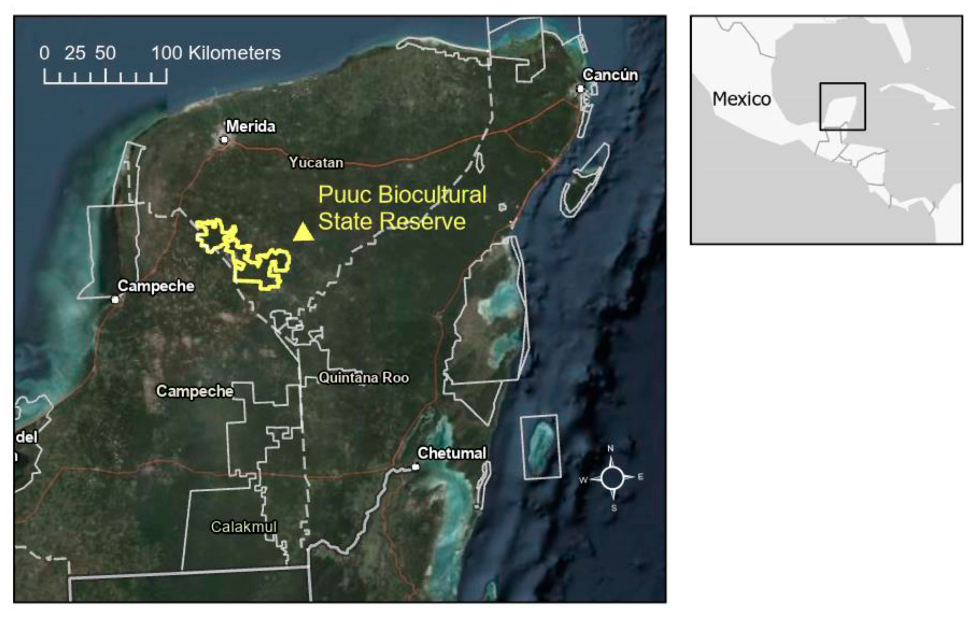
In the case of the Puuc Biocultural State Reserve (PBSR), a tropical dry forest-dominated reserve located in the Central Yucatan Peninsula, Mexico, effectiveness depends on coordinating multiple communities and entities that form this special state park. The PBSR was established in 2011 by the Yucatan State Government primarily as a means to preserve the biological diversity of this tropical dry forest landscape, its carbon sequestration capacity, its historical value for Mayan culture and the sustainable livelihoods persisting in the region [12]. This type of reserve is the first of its kind in Mexico. It covers the territory of five municipalities that have historically been inhabited by low-density human populations dedicated to small traditional agricultural practices (milpas) and cattle ranching in the form of communal properties (ejidos) and private properties. Some of these communities implement sustainable forestry projects as well. The PBSR was established as a corridor connecting the forested areas of the south of Campeche, and Quintana Roo states with the Celestún Biosphere Reserve in northeastern Yucatan [12].

The main activities that cause forest disturbances in the PBSR are agricultural activities such as cattle ranching (which is concentrated in small areas in the north and southeast of the reserve), the cultivation of vegetables such as corn, beans, sorghum and citric fruits, and forestry activities related to charcoal production and house construction. These activities are mostly implemented in milpa systems. Milpa systems are traditional Mayan land management schemes that involve slash-and-burn agriculture of multiple crops. Crops are followed by fallow after at least 4 years, which allows for forest regrowth and soil nutrient recovery (a period called ‘barbecho’).

The PBSR management plan requires community-based planning of all productive activities coordinated by an inter-municipal board. It is important to note that 55% of the reserve is managed by ejidos while the rest are private properties. All activities are planned to minimize environmental impact and safeguard the ecological sustainability needed to preserve the ecosystem services that the region provides to its inhabitants and the surrounding communities [12]. Before its creation, more than 86,000 hectares had been reported as forested areas within the reserve, which represents more than 63% of its extent. The PBSR strives to maintain a tight balance between productive activities and forest conservation through community-based governance. However, the intermunicipal board has also identified threats to this balance. The PBSR has documented forest loss and disturbance through the expansion of cattle ranching (often incentivized by government subsidies), unsustainable forestry and hunting activities, road construction and increased forest clearing due to the shortening of the barbecho or fallow period. The extent to which these activities have transformed the landscape after the creation of the PBSR has not been assessed. More than 10 years after its creation, an assessment of the forest cover dynamics before and after the creation of the reserve can help understand the role of the PBSR in this socioecological system.

Over the past several years, there have been significant advances in the design of continuous land cover change (CLCC) mapping algorithms that take advantage of the high-quality Landsat data archive that became freely available in 2008 [13,14]. CLCC algorithms produce annual land cover change maps showing the location and extent of deforestation events occurred in every single year. In addition, numerous applications have used the power of multispectral and hyperspectral optical, radar, and LiDAR sensors for mapping ecosystem age, biomass and carbon stocks, alpha and beta diversity, biochemical heterogeneity, tree height, vertical structure, and complexity, among other attributes [15]. In tropical forests, state-of-the-art methodologies using multispectral, hyperspectral imagery and/or LiDAR usually achieve R2 values of ~0.5–0.7 for canopy functional trait mapping, while categorical maps of plant functional types can achieve overall accuracies of ~0.8 [16].

In this study, we integrated state-of-the-art remote sensing tools and products for assessing forest clearing dynamics in the context of the forest conservation goals of the PBSR. We analyzed forest clearing dynamics using an original forest loss product derived from the analysis of the time series of Landsat 5, 7 and 8 from the year 2000 until 2021. We compared it to spatially explicit models of carbon density and tree species richness derived by using L-band radar backscatter data, radar texture metrics, and climatic and field data [17]. In the context of the PBSR management objectives, the goal of the study is to answer the following questions: (a) How has the creation of the PBSR impacted the frequency and area of forest loss within its boundaries? (b) Are productive activities contemplated in the PBSR governance model compatible with the maintenance of carbon density and species richness?

2. Methods

2.1. Study Area

The study area was defined as the area within the PBSR boundaries and the adjacent and wider landscape around the reserve (Figure 1). This area was defined by all municipalities intercepting a 25 km area of influence around the PBSR. This included municipalities immediately adjacent to the PBSR and municipalities adjacent to these. Some municipalities extend far beyond the 25 km area of influence and therefore were only represented partially in the analysis. Municipalities completely included in the study area were Oxkutzcab, Santa Elena, Muna, Ticul, Akil and Dzan in the Yucatan state. The study area included partial coverage of the municipalities Hopelchen, Calkini and Hecelchakan in Campeche state and the municipalities of Tekax, Tzucacab, Chacsinkin, Tixmehuac, Teabo, Mani, Mama, Chapab, Sacalum, Abala, Opichen, Kopoma, Maxcanu and Halacho in the Yucatan state.

The vegetation communities in this region are predominantly secondary semi-deciduous forests that can reach a canopy tree height of 15–20 m, losing 50–75% of their leaves during the dry season. Annual rainfall ranges from 1000 to 1500 mm with an annual temperature of 25.9 °C to 26.6 °C. The elevation of the terrain in the area ranges from 60 to 250 m above sea level. The dominant species are Neomillspaughia emarginata, Gymnopodium floribundum, Bursera simaruba, Piscidia piscipula and Lysiloma latisiliquum. The local geomorphology combines flat areas with limestone hills of moderate slopes. The landscape consists mainly of forest land (94% of the area), mostly dominated by forest stands of different successional ages.

2.2. Semi-Automated Forest Disturbance Detection from 2000 to 2021

2.2.1. Generation of a Baseline Map

The detection and mapping of forest loss events were performed using a semi-automated continuous change detection method that involves the user verification of change thresholds for each time step. Overall, the method consisted of detecting changes in vegetation index values every three months over known forested areas (post-classification change detection) from the year 2000 until the end of the year 2021.

First, we produced a baseline forest cover map for an initial time step in the year 2000. We downloaded a cloud-free (<5%) Landsat 5 (L5) scene (20/46) surface reflectance product for a single date (28 March) for the year 2000 using the USGS EROS Science Processing Architecture (ESPA) online interface. Then, we used R packages (raster, rpart, randomForest, gdal and rgeos) for image pre-processing, cloud masking and supervised classification using the Random Forest algorithm.

For classification, we collected training data through on-screen interpretation of the L5 scene in an RGB453 false color composite and very high-resolution imagery available in ArcGIS Online (ESRI), in combination with the INEGI VI Series Land Cover Classification map. We arbitrarily chose a quantity of ~800 locations as the target for training data collection. The number of training polygons per class was calculated through proportional allocation using the original land cover proportions in the INEGI land cover map. The proportional allocation equation used was Sh = (Nh/N) ∗ n, where Sh is the sample size per class, Nh is the class size, N is the total landscape size, and n is the desired total number of samples. A total of 836 polygons were digitized, with 595 polygons for the forest class and 241 polygons for the Non-Forest class. The forest class represented all forest types defined in the INEGI land cover map, and the Non-Forest Class represented anthropogenic land covers and water features. Finally, the Random Forest classifier was performed using visible, near-infrared and short-wave infrared bands as well as a Normalized Difference Moisture Index (NDMI) and a Normalized Burn Ratio 2 (NBR2) products from the L5 scene.

To evaluate the accuracy of the baseline map, we implemented a stratified random sampling approach for generating validation points and an area-based error matrix [18,19]. Through this method, we calculated the overall user’s and producer’s accuracy with error-adjusted area estimates calculated at a 95% confidence interval. Based on the extent of forest/non-forest land covers, we estimated the optimal size of samples per class for accuracy assessment. We used the proportional allocation formula to estimate the number of samples per class. We targeted a total of 800 samples for validation purposes as a match to the number of samples used for training the image classification. The proportional allocation formula resulted in 621 samples for the forest cover and 179 samples for the non-forest cover. Samples were collected using a 250 × 250 m grid over the baseline map in ArcGIS 10.7. Cell grids per class were randomly selected, and each cell’s centroid point was generated. These centroid points were used for map-to-reference data comparisons using Google Earth Pro.

2.2.2. Post-Classification Change Detection

We used a post-classification change detection approach in order to minimize error propagation over the 20-year time series [14]. For post-classification change detection, we used the Normalized Burn Ratio 2 (NBR2) vegetation index products from Landsat 5, Landsat 7 and Landsat 8 SR tier 1 image collections. We used the NBR2, given its overall better performance than other indices in detecting a change in tropical dry forests, as evidenced by Smith et al. [20] for the same study area. Other authors have also reported improved performance from using NBR2 for detecting forest change in time series of remotely sensed data [21,22]. Using Google Earth Engine (GEE), we filtered Landsat imagery to four quarters every year from 31 January to March (Q1), 1 April to 30 June (Q2), 7 July to 30 September (Q3) and 1 October to 31 December (Q4). For each quarter, we selected only clear observations, masking clouds and cloud shadows to every scene using the pixel qa product, and generated a composite of maximum NBR2 values for every quarter.

Each NBR2 quarter composite was inspected in ArcGIS, and a threshold for values that were <−1.5 standard deviations from the mean was applied in order to isolate non- or little vegetated surfaces. The threshold was a generalized approximation to the 1.65 thresholds used by Hamunyela et al. [23]. We inspected the ability of the 1.65 thresholds to depict non-vegetated areas and determined that 1.5 was slightly more conservative and provided a better delineation of non-vegetated areas using the NBR2 product. This process was done interactively through visual inspection and manual thresholding in ArcGIS. In some cases, thresholds were slightly adjusted to values between <−0.5 and <−1.5 standard deviations to match the exact dimensions of non-vegetated surfaces. Variations of this standard deviation threshold were used to improve the delineation of areas with negative NBR2 values that appear to be probable forest disturbance events. Binary maps of vegetated (0) and non-vegetated surfaces (1) were generated. These products, however, did not represent the final forest disturbances for a given year.

We subtracted these rasters from the forest mask of the previous year in order to isolate forest disturbances. We then added all quarter forest disturbance masks in order to produce annual forest disturbance maps. Following Hamunyela et al. [23], we flagged forest disturbances only after two or more consecutive observations of low NBR2 values, and in some cases, we allowed all possible observations to be included in the annual product. This was done given that cloud contamination and L7 missing data affect the probability of detecting consecutive observations. Changes in quarter NBR2 values following the cultivation of recently cleared land can also mask the detection of these consecutive observations. Isolated pixels were successfully filtered using a focal 3 × 3 majority filter leaving the more regularly shaped forest disturbances intact. For every time step, we achieved a final annual product only after satisfactory visual inspections. Final deforestation polygons were limited to areas larger than 0.18 ha in order to eliminate spurious isolated pixels.

To assess the accuracy of the annual forest-clearing product, we implemented a two-stage cluster sampling design to generate validation locations. Using a 5 km × 5 km grid, we calculated the percentage of forest clearings detected per cell using the combined annual forest clearing dataset. This allowed us to generate a grid with forest clearing percentages. We categorized the grid using the Jenks optimization method (Natural breaks) in ArcGIS in four classes stable forest or no loss (128 cells), low forest loss (1005 cells), intermediate forest loss (194 cells) and high forest loss (29 cells). We then used the Neyman optimal allocation formula [24], which takes into account the number of cells and the standard deviation of forest cleared area per cell, to calculate the number of sampling points per class needed for validation in 25% of the landscape. We targeted 800 samples for validation purposes as a match to the number of samples used for training the image classification and for validation of the baseline map. The Neyman optical allocation method estimated that proper representativeness of the landscape would require selecting 9 cells in the stable forest class, 627 in the low clearing class, 124 in the intermediate clearing class and 40 in the high clearing class. Within these sets of cells, we re-calculated the area with stable land use and land cover (no forest cover change) and with forest change (forest clearings) and further estimated the number of sampling points needed for validation by proportional allocation. This resulted in 593 sampling points generated to cover stable land cover and 207 sampling points to cover the forest-loss class (for a total of 800 validation points). Each of the samples was individually inspected in Google Earth Pro, and using the historical imagery tool, we looked for evidence of change between 2000–2021 to validate the map class. An area-weighted confusion matrix was used to compute overall producer’s and user’s accuracies, along with standard errors and forest clearing areas estimated at a 95% confidence interval [25,26].

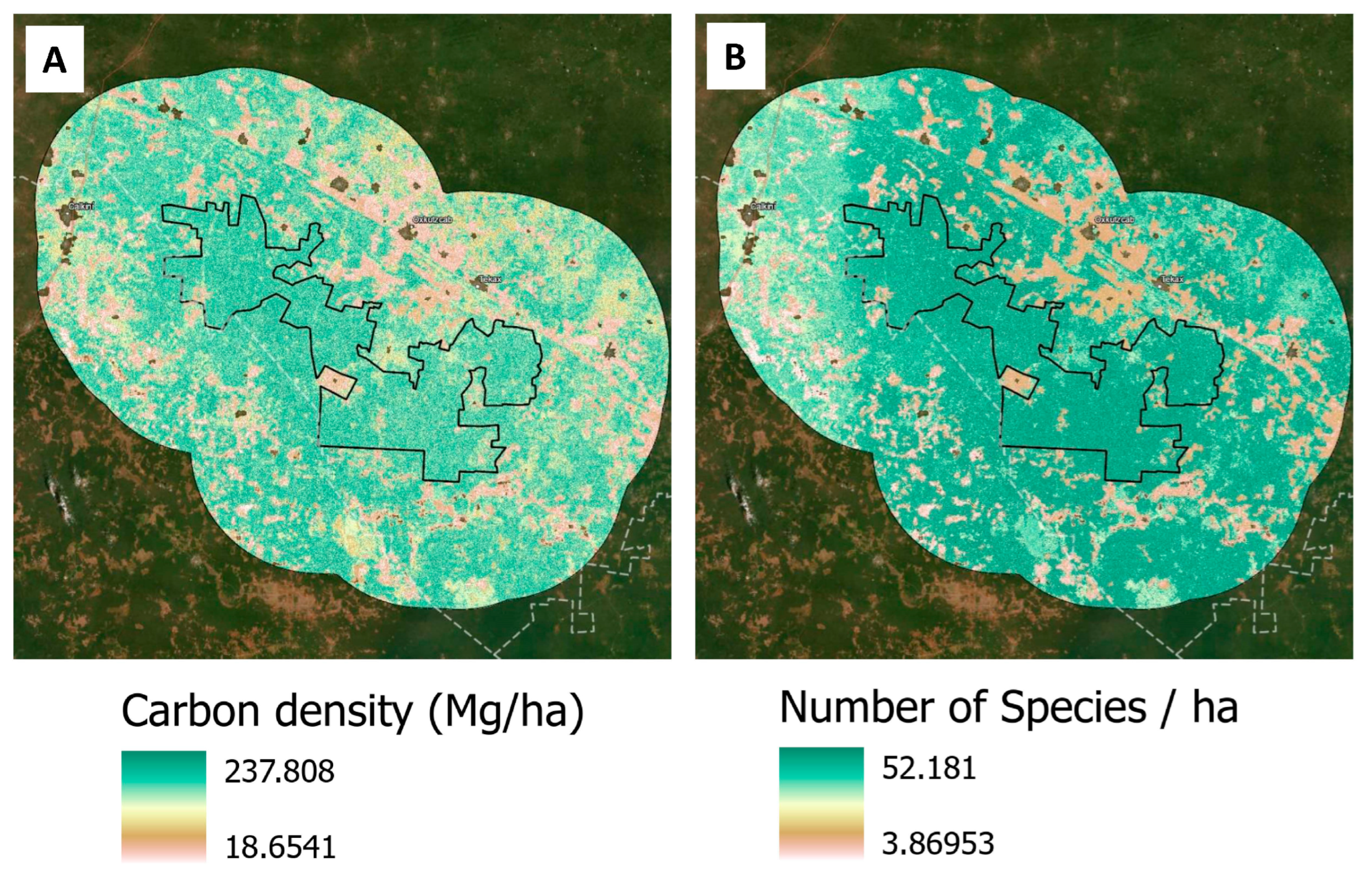
2.3. Carbon Density and Tree Species Richness Models

The methodology to derive carbon density and species richness maps for the study area is thoroughly explained in Hernandez-Stefanoni et al. [17]. In their study, authors generated spatial models of tree species richness and carbon density for the entire Yucatan Peninsula of Mexico (Figure 2). Field data on tree species richness and aboveground biomass (Mg/ha; used as a measure of carbon density) was obtained from the National Forest Inventory (NFI) of Mexico from surveys conducted between 2009 and 2014. A total of 2847 plots were used, and these were distributed in the forested areas in a stratified sampling scheme depending on the vegetation type. Each field plot consisted of four circular 400 m² sub-plots distributed within an area of 1 ha. All trees with a diameter at breast height (DBH, 1.3 m) ≥7.5 cm were identified at the species level, and their diameters and heights were measured. AGB stocks per plot were calculated in standard units (Mg ha⁻¹) using local and regional allometric equations, which were developed by vegetation type, plant growth form and DBH size.

The study used ALOS-2 PALSAR-2 (Advanced Land Observing Satellite Phased Array L-band Synthetic Aperture Radar) mosaic tiles for the year 2015—with 25 m resolution and dual polarization (HH and HV) preprocessed for orthorectification, slope correction, and radiometric calibration. It used backscatter coefficients (γ°) and Normalized Difference Backscatter Index (NDBI) products, as well as variability in backscatter values among pixels using texture metrics and climatic water deficit (CWD) data. This process generated 24 variables, considering eight texture metrics and three bands (HH, HV and NDBI) that were used for AGB and species richness estimations. A random forest regression model was used to estimate the spatial distribution of AGB and tree species richness from all explanatory variables. Model validation of the regional maps obtained herein using an independent data set of plots resulted in a coefficient of determination (R²) of 0.28 and 0.31 and a relative mean square error of 38.5% and 33.0% for aboveground biomass and species richness, respectively, at the pixel level.

2.4. Statistical Analysis

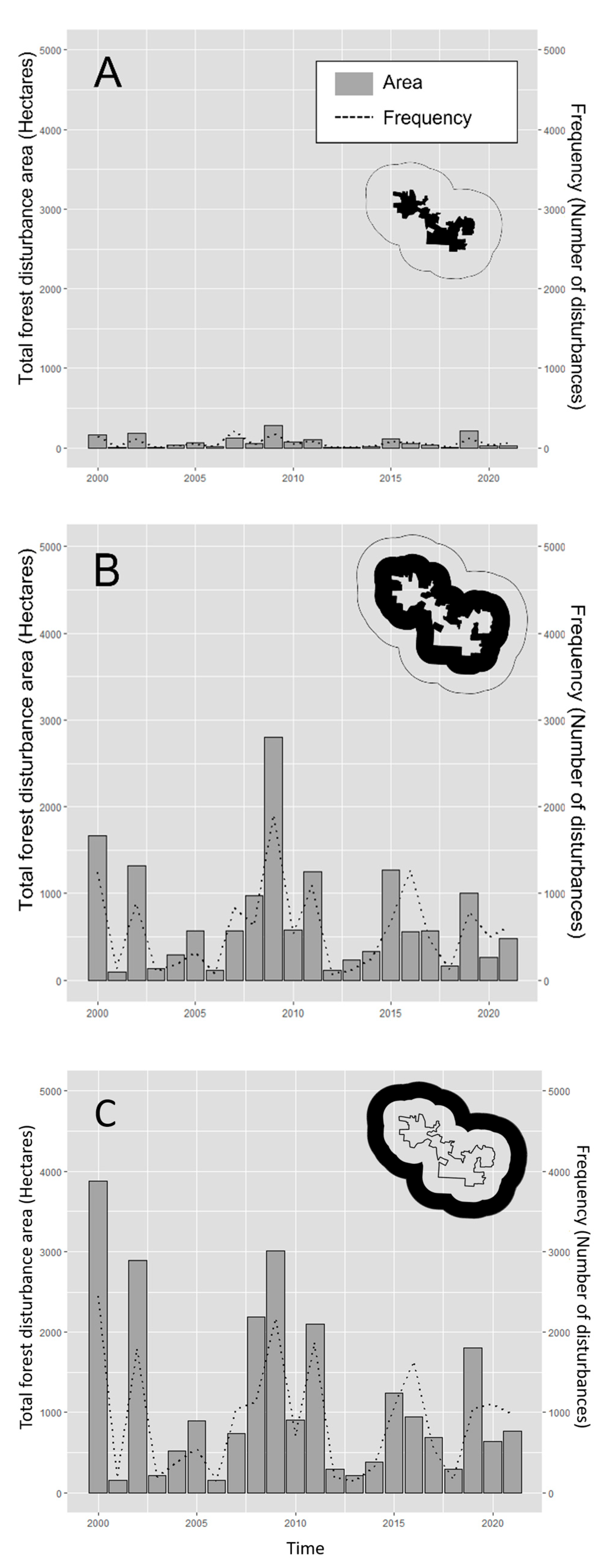
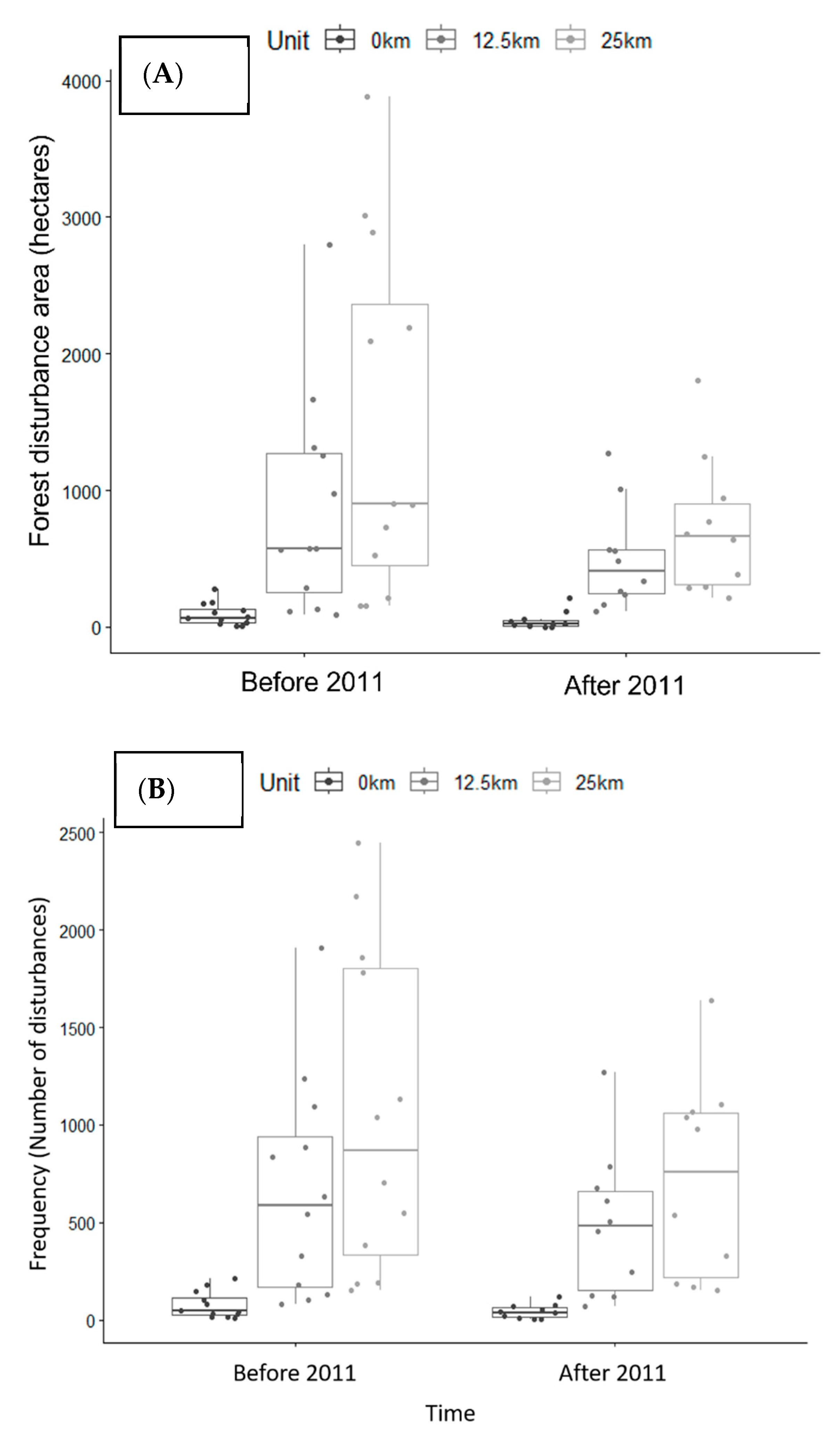
In order to assess whether the creation of the PBSR has impacted the frequency and area of forest loss within its boundaries, we calculated basic statistics on the number of forest clearing events per year (frequency) and forest loss per year (in hectares/year) in three different geographic analysis units before and after the year 2011 (date of its creation): inside the PBSR boundaries, in a 12.5 km buffer ring around the PBSR boundaries and in a 25 km buffer ring around the PBSR. The two buffer distances were arbitrarily selected in order to compare forest clearing dynamics in the communities within the PBSR and the communities around it. We then performed pairwise comparisons between geographic analysis units before and after 2011 using the Kruskal–Wallis rank sum test (kruskal.test()) in R software version 2023.03.0.

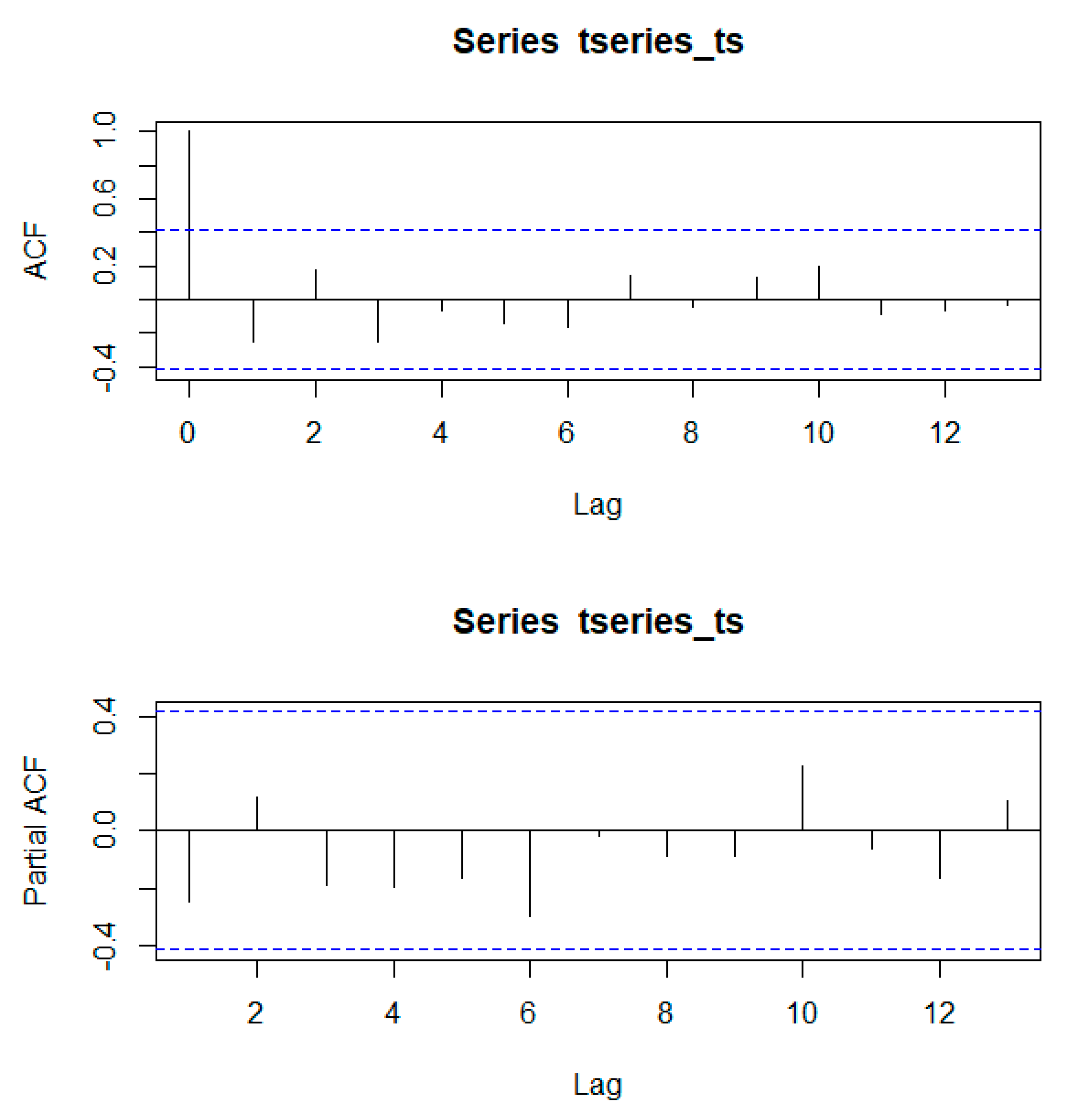
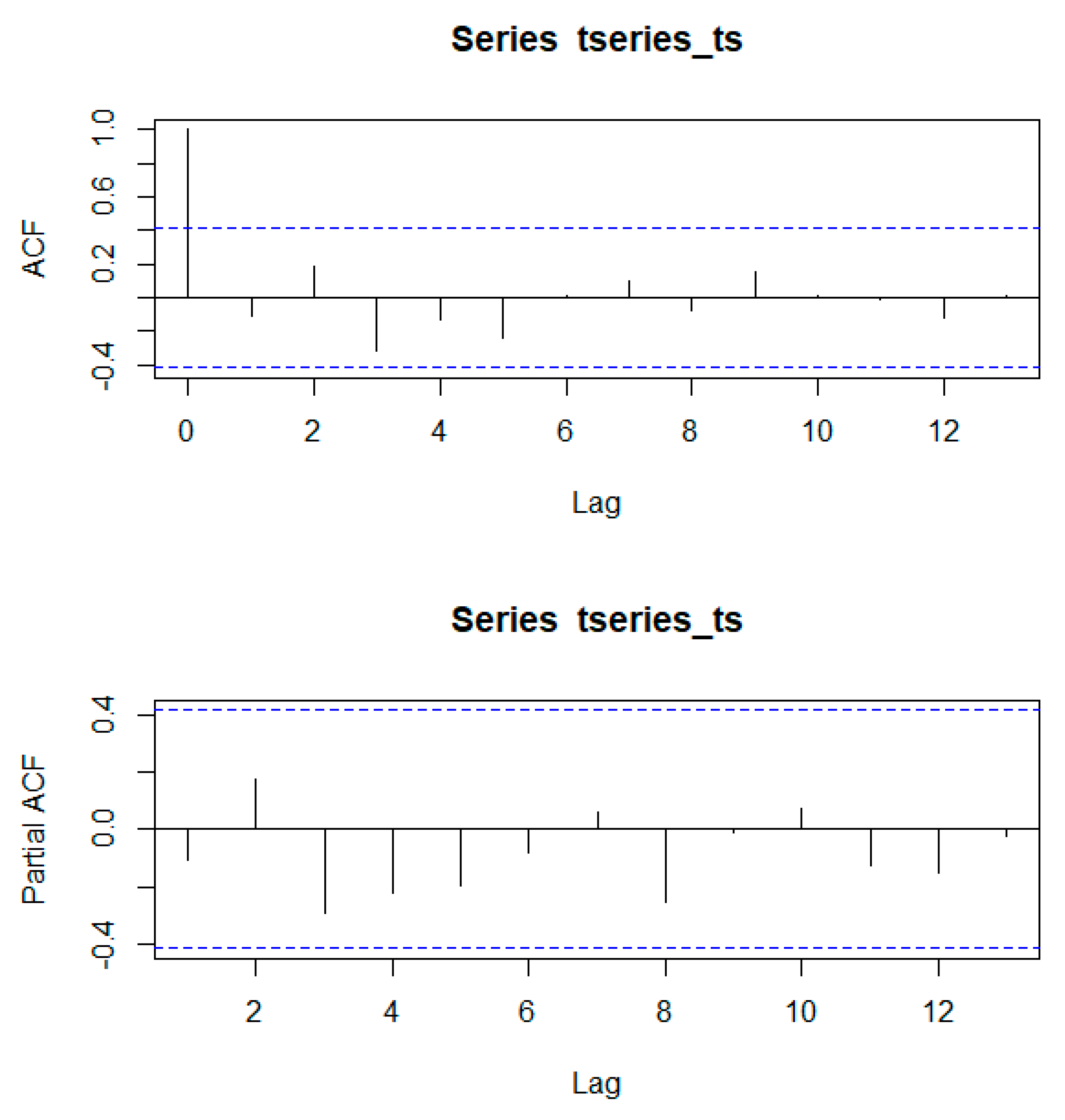
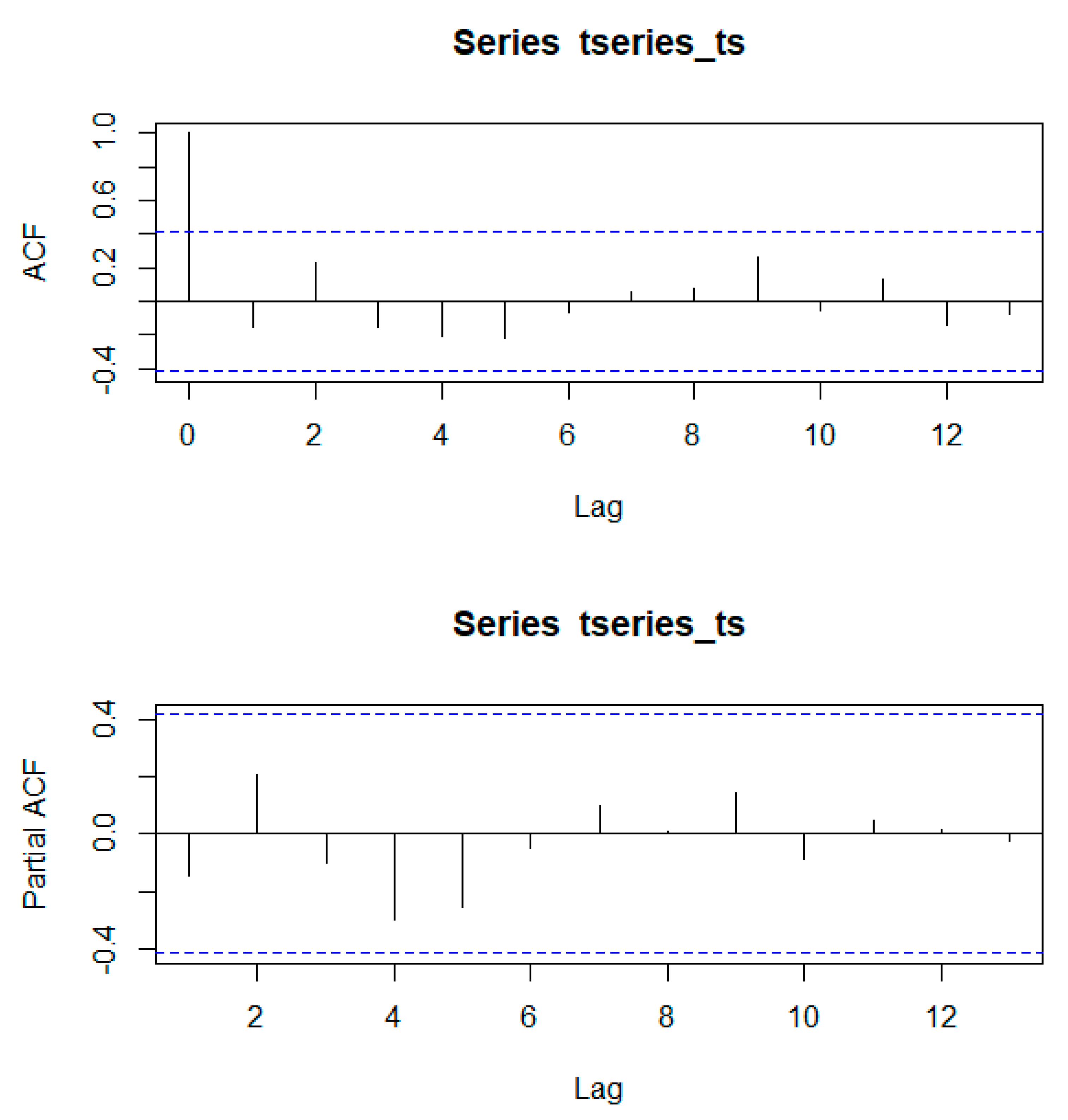
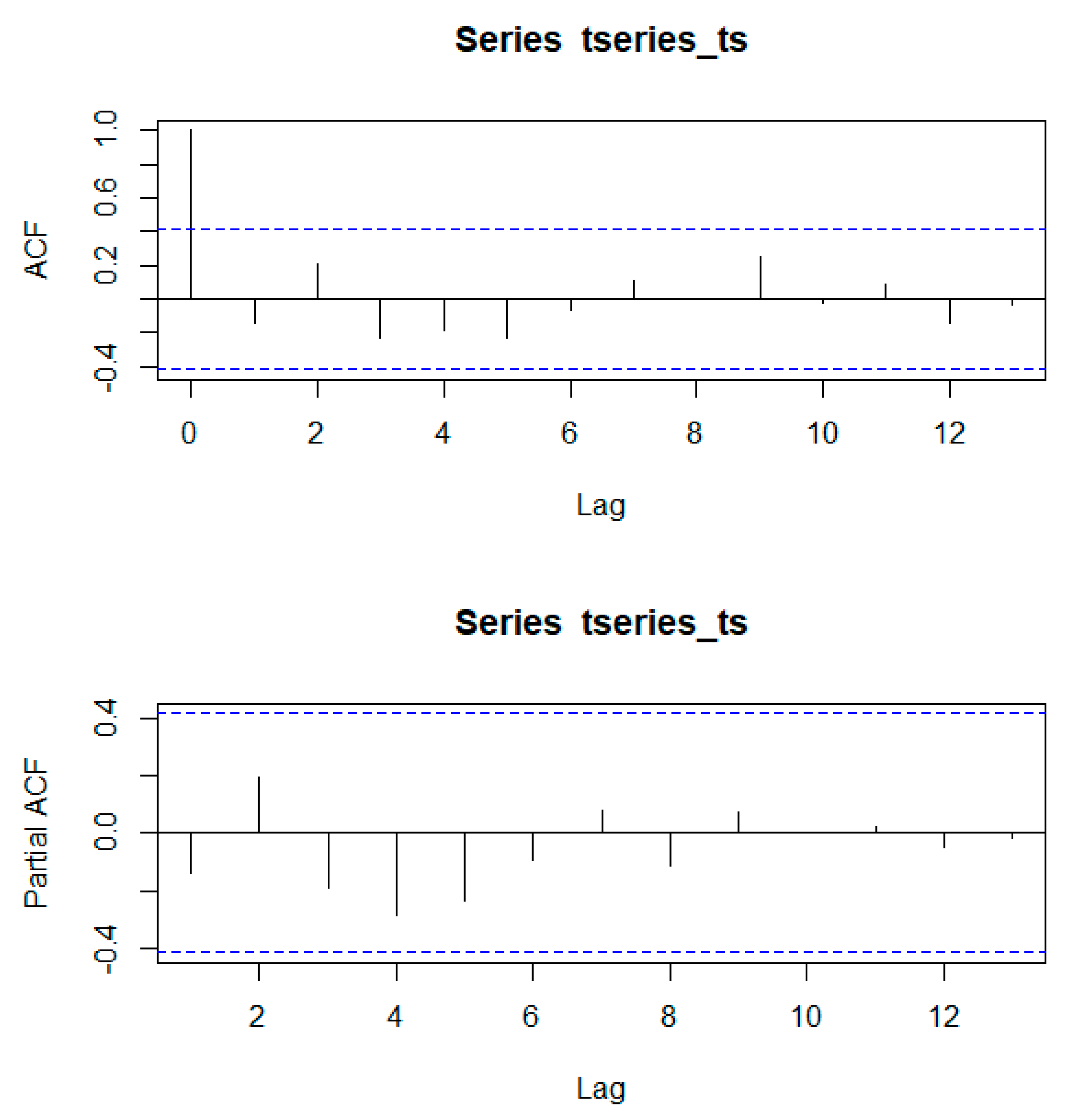
Using the Mann–Kendall trend statistic package (Kendall) in R, we also investigated if there were significant trends in the time series of annual forest area and evaluated whether these trends were different before and after the creation of the PBSR. Before its application, we used the acf() and pacf() functions in R to test for autocorrelation and partial autocorrelation in the time series. Appendix A shows that autocorrelation present in the series was not significant at any scale.

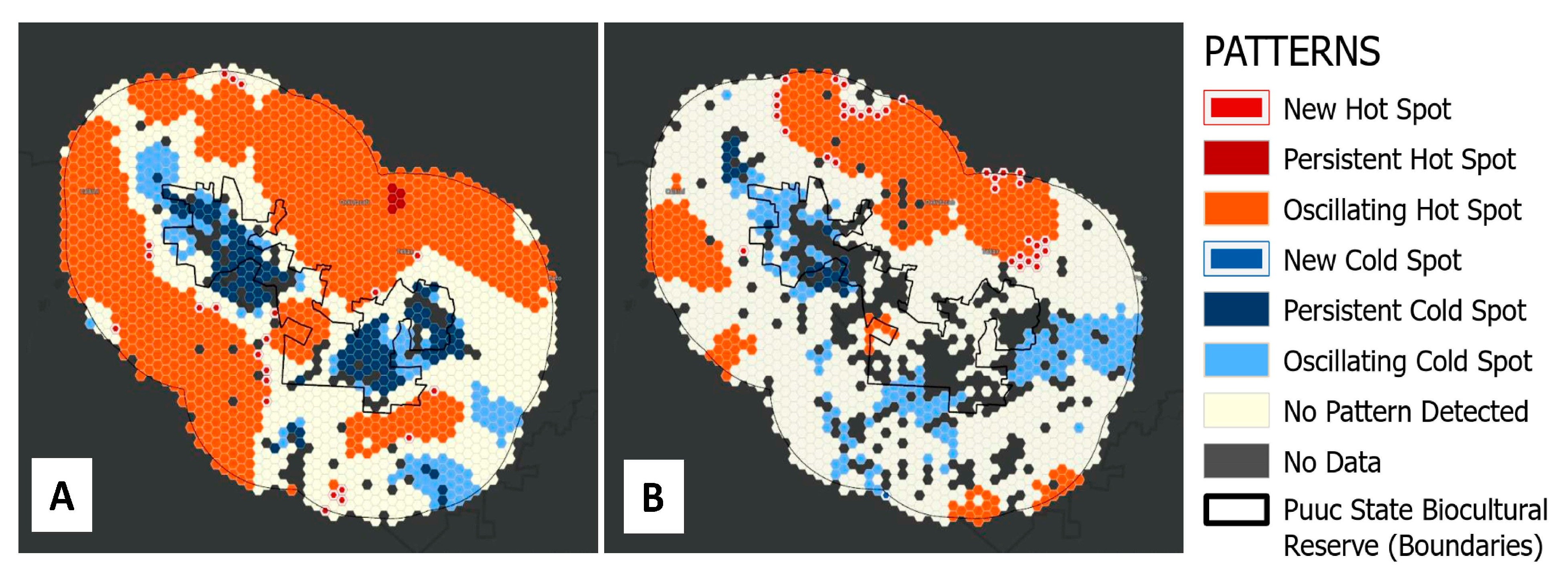
In order to further investigate if there were significant spatiotemporal patterns in the frequency of forest clearing events before and after the creation of the PBSR, we used the ‘Emergent Hotspot Analysis’ or EHSA tool in ArcGIS Pro (ESRI). The EHSA tool aggregates point into space-time bins. Aggregation of points per year was performed at a 2.5 × 2.5 km bin size in one-year intervals using hexagon grid cells. To get a measure of the intensity of feature clustering in each bin, the hotspot analysis uses a space-time implementation of the Getis-Ord Gi* statistic, which considers the value for each bin within the context of the values for neighboring bins in space and in time [27]. We selected only adjacent bins (6) to each hexagon cell as neighboring bins and a temporal frame of three time steps (3 years). The time series of Getis-Ord Gi* z-scores for each bin and its spatiotemporal neighbors is then assessed using the Mann–Kendall statistic. The result from this analysis is a clustering trend z-score, p-value, and binning category for each location. Binning categories are based on the intensity of the clustering (Z-scores and p-values) for a high number of forest clearing events (hotspots) and low numbers of forest clearing events values (cold spots). Hotspots and coldspots are automatically classified into new, consecutive, intensifying, persistent, diminishing, sporadic and oscillating bin categories based on clustering patterns in time and space.

We then assessed whether the PBSR governance model minimizes the impact of productive activities on forest carbon density and tree species richness. For this, we selected only the annual forest loss detected after 2015 (the year of our reference biomass and diversity map) and calculated the mean carbon density and the mean tree species richness for each forest clearing polygon from 2015 until the year 2021. Using a Kruskal–Wallis rank sum test implemented in R, we tested for differences between the distribution of carbon density and species richness values in forest loss polygons and an equivalent random sample in stable forest areas for two geographic analysis units: within the PBSR and outside of the PBSR up to a surrounding area of 25 km distance from its boundaries.

3. Results

3.1. Forest Cover Baseline and Annual Forest Clearing Dataset

The semi-automated classification of the Landsat 5 scene surface reflectance product for 28 March 2000 allowed us to produce a forest cover map that was used as a baseline for detecting changes in forest cover on an annual basis (Figure 3). The baseline forest map was evaluated using a confusion matrix that showed a high overall accuracy of 94%, with a producer’s accuracy of 62.7% for the forest class, 91.5% for the non-forest class, and a user’s accuracy of 96.8% for the forest class and 82.6% for the non-forest class (

Table 1. Area weighted confusion matrix showing the result of the accuracy assessment performed on the forest baseline map for the year 2000 and the annual forest clearing dataset.

Baseline Forest Cover Map (Year 2000).
	Forests	Non-Forests	Total Area Proportions	Total Number of Samples
Forests	0.77	0.02	0.79	621
Non-forests	0.03	0.17	0.2	179
Estimated Area Proportions	0.81	0.18	0.99	800
Class Area Estimates (hectares)	775,845.40	173,146.82
Standard Error of Area Estimates	0.01	0.01
Standard Error of Area Estimates (hectares)	7653.58	6879.07
95% Confidence Intervals in Ha	15,001.02	13,482.98
Overall Percent Accuracy (%)	94.01
Unbiased Accuracy	User’s Accuracy (%)	Producer’s Accuracy (%)
Forest	96.8	62.7
Non-Forest	82.7	91.5
Annual Forest Clearing Map (2000–2021)
	Forests	Non-forests	Total Area Proportions	Total number of samples
Forests	0.71	0.04	0.75	593
Non-forests	0.05	0.20	0.25	120
Estimated Area Proportions	0.76	0.24	1	713
Class Area Estimates (hectares)	728,066.66	230,511.34
Standard Error of Area Estimates	0.01	0.01
Standard Error of Area Estimates (hectares)	10,706.81	11,687.72
95% Confidence Intervals in Ha	20,985.34	22,907.94
Overall Percent Accuracy (%)	90.95
Unbiased Accuracy	User’s Accuracy (%)	Producer’s Accuracy (%)
Forest	95.9	53.9
Non-Forest	76.9	83.2

). Because the land cover matrix is diverse and includes tree plantations and horticultural crops, pixels representing these land uses would likely be included in the forest class, and vice versa; forest class pixels representing early successional stages would likely be included in the non-forest class. Nonetheless, we considered the accuracy of the map as satisfactory for delineating the overall forest cover distribution by the year 2000.

The map shows that the total error-adjusted estimated area of forest cover for the year 2000 was 775,846 ha (±15,001 ha at a 95% confidence interval), representing 79.9% of the total terrestrial landmass of the study area, which includes the PBSR and a surrounding buffer of 25 km. Forests are distributed evenly across the study area, with the largest continuous fragments found near and within the PBSR. Non-forest areas are represented mostly by rural anthropogenic settlements, towns and small agricultural developments (mostly milpa) along Highway 184 in the northeastern part of the study area in the state of Yucatan. The northwestern part of the study area, in the state of Campeche, also has large areas of non-forested land represented mostly by intensive agriculture developments and towns along Highway 180.

The annual deforestation dataset was successfully generated with an overall accuracy of 91% (Table 1). The matrix shows that the forest clearing class had a moderate rate of commission errors (user’s accuracy of 76.9%), which means areas of no change were counted as forest cover change on a 23.1% rate, while it shows a lower rate of errors of omission (producer’s accuracy of 83%). We considered the results satisfactory for showing overall forest clearing trends spatially and temporally and comparable to other studies at a similar geographic scale [28,29].

The estimated error-adjusted area of detected annual forest clearings from the year 2000 until the year 2021 was 230,511 ha in total (±19,979 ha). Results also show a mean and median forest clearing patch area of 1.26 ha and 0.54 ha, respectively (Std Dev = 3.36), ranging from patches of 0.20 ha to large forest clearings of 229 ha. The majority of patches (98%) fall within the 0.20–7.27 ha range, with the rest falling mostly under 50 ha and only five patches greater than 100 ha.

3.2. Comparisons by Geographical Unit and Time Period

Over the entire study area, annual forest clearings occurred on an average of 1552 clearings per year with an average area of 1951 ha per year. The extent of deforestation peaked for the year 2009 with 6237 ha of forest cleared in 4272 events. The year with the lowest forest clearing detected was 2001, with only 261 ha of forest cleared. In general, the dynamics of forest removal were highly variable during the whole study period. We observed the highest and the lowest forest area cleared during the first ten years. After 2011, clearings peaked in 2019, with 3154 ha cleared in 1948 events. Spatially, clearings were mostly clustered outside the boundaries of the PBSR and less frequent inside the PBSR (Figure 3). Most of the clearing patches greater or equal to 50 ha (n = 22) were located in the southeastern and eastern part of the study area inside or near the state of Campeche and on the northern part of the study area in the state of Yucatan. In Campeche, all of these corresponded to clearings in landscapes dominated by commercial mechanized agriculture, while in Yucatan state, these corresponded partially to large contiguous patches of milpa agriculture and some dedicated to commercial mechanized agriculture.

When analyzed by geographical unit (inside the PBSR and in buffer rings of 12.5 km and 25 km around the reserve), forest clearing dynamics greatly differed (Figure 4). Dynamics were very low and stable inside the PBSR during the whole study period (Figure 4A). The average forest clearing area inside the PBSR was 73 ha per year from an average of 60 events per year (for an average of 1.21 ha per clearing patch). The maximum area cleared was recorded for 2009, with 280 ha in 180 clearing occurrences. In the 12.5 km buffer, annual forest clearing was higher, with an average of 698 ha cleared per year and an average of 582 clearing occurrences per year (for an average of 1.19 ha per clearing patch). Similarly, the peak forest area cleared was recorded for the year 2009 in the 12.5 km buffer, with 2797 ha cleared in that year. In the 25 km buffer, the magnitude of the area cleared and number of occurrences was higher for the years 2000, 2002, 2008, 2009 and 2019 in comparison to the other geographical units of analysis (Figure 4C), with the largest area cleared registered for the year 2000 and followed by the year 2009. Kruskall–Wallis tests showed that forest clearing area and frequency per year were significantly different between geographical units (

Table 2. Summary of results from Kruskall–Wallis Rank Sum tests and Mann–Kendall trend tests.

Kruskall–Wallis Rank Sum Tests	Χ2	df	p-Value
Forest clearing (ha)
By geographical unit (inside, 12.5 km, 25 km)	37.97	2	<0.001
By time period(before or after 2011)	1.06	1	0.3029
Frequency of forest clearing events
By geographical unit (inside, 12.5 km, 25 km)	38.41	2	<0.001
By time period(before or after 2011)	0.89	1	0.3439
Carbon density (Mg/ha)
In Forest clearings vs. Random selection (Inside PBSR)	60.12	1	<0.001
In Forest clearings vs. Random selection (Outside PBSR)	1213.7	1	<0.001
Number of species per hectare
In Forest clearings vs. Random selection (Inside PBSR)	85.05	1	<0.001
In Forest clearings vs. Random selection (Outside PBSR)	3422.1	1	<0.001
Mann–Kendall trend tests	Score	tau	p-value
Forest clearing (ha)
Inside (Pre 2011)	16	0.24	0.30367
Inside (Post 2011)	4	0.06	0.83701
12.5 km buffer (Pre 2011)	16	0.24	0.30367
12.5 km buffer (Post 2011)	11	0.24	0.37109
25 km buffer (Pre 2011)	12	0.18	0.45067
25 km buffer (Post 2011)	15	0.33	0.2105
All (Pre 2011)	16	0.24	0.30367
All (Post 2011)	15	0.33	0.2105

). Figure 5 shows the differences in the ranges of forest area and frequency between geographical units before and after the creation of the PBSR in 2011. In general, we observed a general shift in the magnitude of forest cleared before and after the creation of the PBSR, especially outside of the PBSR, but the differences were not significant in these two time periods for any of the geographical units (Table 2).

The Mann–Kendall trend tests showed no temporal trends detected in the area cleared during the whole study period for the three geographical units (Table 2). There was also no evidence of significant positive or negative temporal trends in forest area clearing dynamics before and after the creation of the PBSR, either inside of the reserve or in the 12.5 km and the 25 km buffer rings (Table 2).

3.3. Emergent Hotspot Analysis

Emerging trends were assessed using the space-time hotspot analysis in order to investigate whether the creation of the PBSR impacted the spatiotemporal trends in forest clearing. The analysis is presented for forest clearings detected between 2000 and 2011, and between the 2012–2021 period. Figure 6 shows the results of this analysis and depicts the distribution of areas of stable low clearing intensity (e.g., persistent cold spots: low frequencies and clustering maintained in time and space during the period of study) and stable high intensity (e.g., persistent hotspots: high frequency and clustering maintained in time and space during the period of study) of forest loss events. It also shows areas where recent increasing trends and decreasing trends in forest clearing clustering are occurring (e.g., new hotspots and cold spots) and where high clustering occasionally happens (e.g., oscillating hotspots and cold spots). Areas that were not categorized or deemed to have insufficient data did not record any significant trend across the years.

Results indicate a widespread occurrence of oscillating high-intensity areas before 2011, with one cluster of persistent hotspots in the northern part of the study area. Before 2011, newer or recent hotspots were spread out across the study area. Persistent and oscillating low-intensity cold spots were evident in the central part of the study area corresponding with the eastern and western sections of the PBSR. After the creation of the PBSR in 2011, stable high-intensity areas were less frequent and were present in smaller ranges around towns in the northern part of the study area and some locations in the southern area that correspond to the state of Campeche. We observe, after 2011, a reduction of the hotspots in the middle of the PBSR and more empty cells all across the PBSR, which means there were no sufficient forest clearing data to compute the spatiotemporal statistical analysis. There were also fewer persistent cold spots inside the PBSR after 2011. New hotspots after 2011 are mostly located in the northern part of the study area.

3.4. Comparison to Carbon Density and Species Diversity Models

Results show that slash-and-burn activities select areas of lower carbon density and species richness in comparison to what is available. This pattern was detected inside and outside the PBSR. Figure 7 shows histogram comparisons of the frequency of forest clearing events by carbon density and species richness ranges. Frequencies are compared between carbon density and species richness in forest clearing polygons after 2015 and a similar number of random locations in forested areas. Inside the PBSR, forest clearing events cluster around the 99–150 Mg/ha carbon density range and the 33–40 species/ha range. Outside the PBSR, forest clearing is more widespread and occurs around 42–152 Mg/ha. It also occurs in a bimodal pattern in relation to tree species richness with a cluster in the ranges of 11–19 species/ha and 27–41 species/ha. The Kruskall–Wallis tests show that the distribution of forest clearing events is significantly different from random in all pairwise comparisons (Table 2) and is shifted towards lower values in clearings, especially outside the PBSR (Figure 7).

4. Discussion

The implementation of a semi-automated method for mapping annual forest clearings for the 2000–2021 period using the Landsat archive allowed us to accurately quantify forest cover change dynamics inside and outside the PBSR. However, results from the accuracy assessment suggest that omission errors were high for the forest class in the 2000 baseline map (Producer’s accuracy of 62.7%) and for the annual forest clearing dataset (producer’s accuracy of 53.9%). This omission error rate might indicate an underestimation of forest clearing activities and suggest that the conversion of forests to milpa and other anthropogenic land uses might be occurring at a higher frequency. The use of a post-classification change detection method using NBR2 thresholding might have underestimated the occurrence of a forest clearing in some instances. This could happen if, after moderate to high rainfall events or land irrigation, a quarter quantification of the NBR2 threshold does not accurately reflect the separation between forest cover and anthropogenic land uses. This masking effect could occur given that NBR2 uses short-wave infrared bands highly sensitive to surface water content.

In spite of these potentially omitted clearing events, the dataset registered 34,138 forest-clearing events in a pattern consistent with the spatial distribution of slash-and-burn activities expected for landscapes undergoing socioecological processes where a conservation area has been in place. The unbiased (error-adjusted) estimation of the total forest area cleared during the 2000–2021 period was 230,511 ha (±19,979 ha), which adjusts estimates based on omission errors and commission errors calculated in the accuracy assessment.

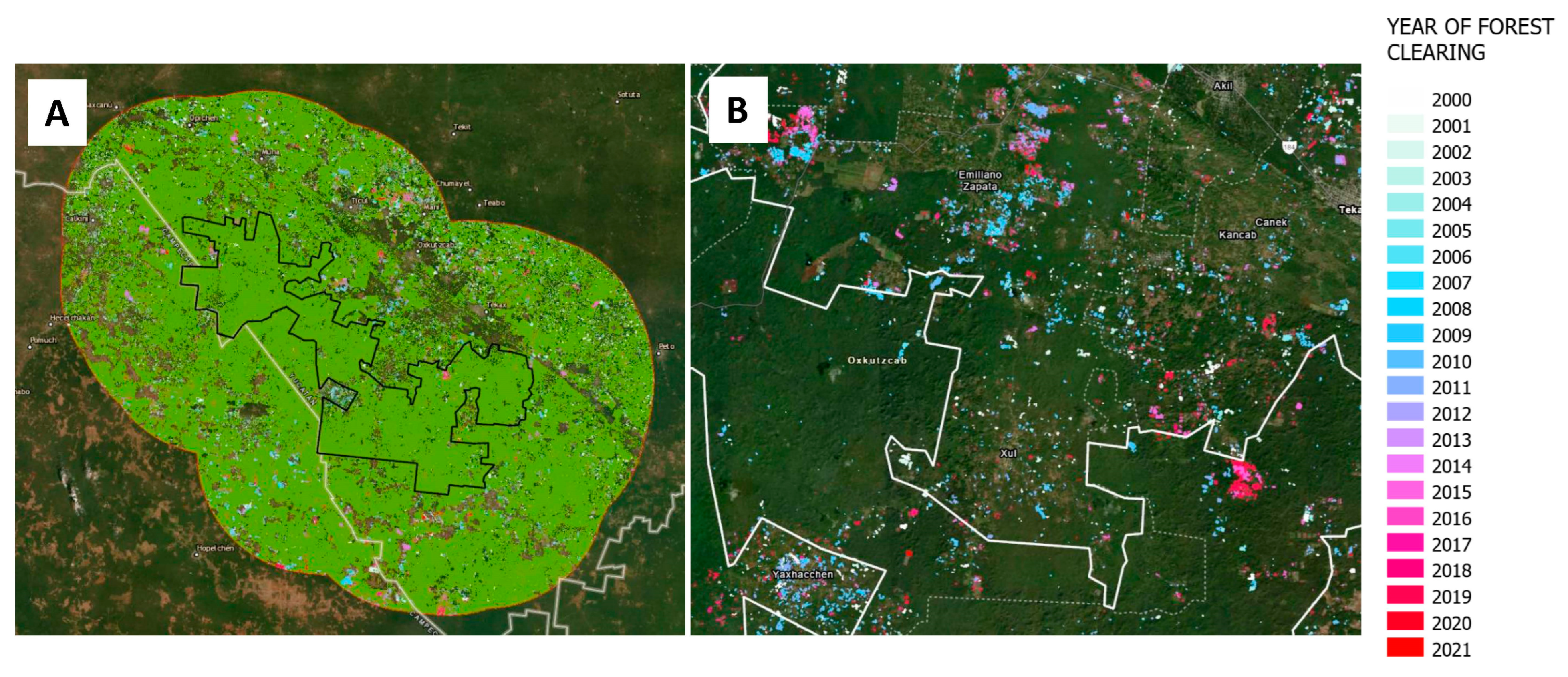
Regarding the impact of the creation of the PBSR on the area and frequency of forest clearings, our results suggest that although forest clearing was significantly more intensive outside of the PBSR than within the PBSR during the entire 2000–2021 period, there is no evidence suggesting that the frequency and magnitude of forest clearing changed over the years after the creation of the PBSR in 2011. Figure 4 and Figure 5 show slight differences in the magnitude of forest-clearing events from 2000 to 2021, but this pattern was evident only for the 25 km buffer ring outside the PBSR. In fact, the Mann–Kendall trend statistics suggest there is no trend in the annual forest clearing time series in any of the geographical units (entire study area, inside PBSR, in the 12.5 km buffer ring and in the 25 km buffer ring) and for any of the time periods (pre-2011 and post-2011). The EHSA analysis does show, however, that forest clearing clustering (hotspots) during the 2012–2021 period was less common than prior to 2011 and that these new hotspots have been confined to areas outside the PBSR (Figure 6). In fact, the EHSA analysis was unable to find sufficient forest clearing data in numerous cells within the boundaries of the PBSR that would yield any significant spatiotemporal trend during the 2012–2021 period, which means forest clearing occurred less often within the PBSR. EHSA results, therefore, suggest lower forest clearing intensity in recent years for the study area, which could be a minimizing effect of the PBSR on the frequency of forest clearing events inside the reserve. However, this could also be a product of landscape-scale processes not linked to the creation of the PBSR, such as migration and socioeconomic processes [12]. Understanding the underlying drivers behind these patterns will need further research.

For the 2000–2021 period, published literature and national reports show mixed results regarding the trends in forest clearing for the Yucatan peninsula. Krylov et al. [30] report a higher annual rate of deforestation for the Yucatan Peninsula in comparison to national rates. Previous research by Portillo-Quintero and Smith [31] also lists the Yucatan Peninsula as one of the largest hotspots of forest clearing in the Mesoamerican region. [32] estimated forest losses of up to 85% in multiple individually managed and parcelized ejidos in the Yucatan state between 1985 and 2016. Nonetheless, Ellis et al. [33] indicate that even though annual deforestation is high in the State of Yucatan, it remains lower than in Quintana Roo and Campeche. When observed at the scale of the PBSR and its surroundings, a rapid report using the public online portal of the Global Forest Watch shows that tree cover loss in the same study area (PBSR and its surroundings) does not follow a negative or positive trend and has been stable since the year 2001 until the year 2021. These results indicate that the study area has experienced lower deforestation rates compared to the reported statewide and regional deforestation processes in the Yucatan peninsula. Our results also show that forest clearing activities have remained low and stable within the PBSR, and although more frequent than within the PBSR, forest clearing has remained stable in the surroundings of the PBSR.

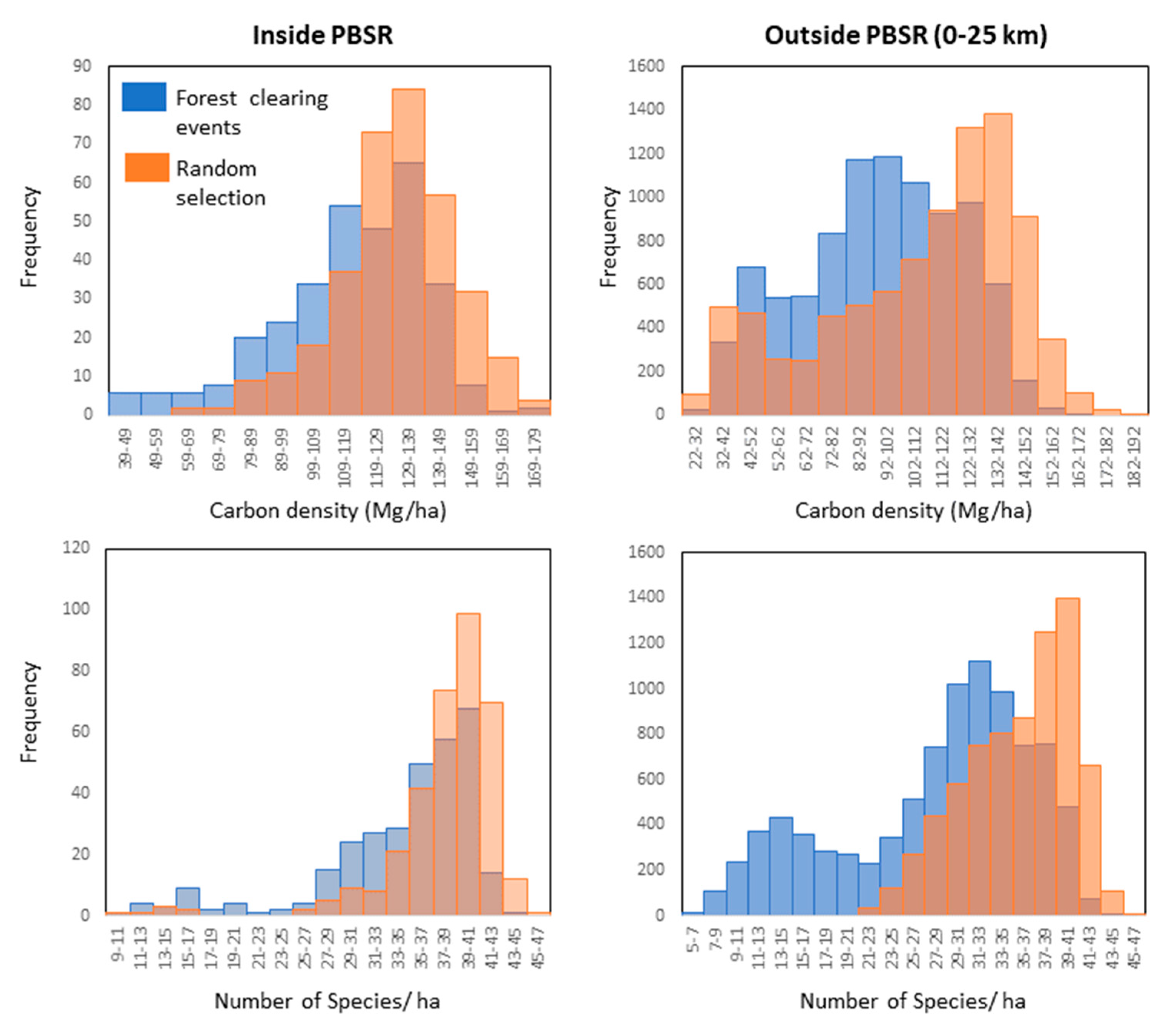
The comparison of the annual forest clearing dataset to remotely sensed carbon density and tree species models further reveals that the PBSR is controlling agricultural dynamics within its boundaries. Our results show that landowners are clearing forests with lower carbon density and tree species diversity in relation to what is available for them at the landscape scale. This is expected given that milpa systems target early to intermediate secondary forests after several years of abandonment (barbecho). However, our data indicate that carbon density and species richness in cleared areas were generally lower (more skewed to the left) relative to random sites outside the PBSR than inside (Figure 7), suggesting that landowners within the PBSR might be practicing longer barbecho periods thereby allowing forests to gain higher carbon density and tree species diversity before slash-and-burn compared to landowners outside the PBSR. Allowing a longer barbecho period is an important component of the traditional shifting cultivation strategy that allows the recovery of soil fertility and results in crops of higher yields [34]. Bray et al. [35] reported similar patterns in the milpa systems of Central Quintana Roo, where longer barbecho periods and the maintenance of late secondary forests are attributed as causes for lower observed deforestation. The PBSR management plan clearly indicates that the practice of short barbecho periods threatens the maintenance of biodiversity and sustainability of agricultural systems in the region and, therefore, promotes the use of longer barbecho periods.

5. Conclusions

Since its creation in 2011, the management goal of the PBSR has been to preserve sustainable livelihoods for the ‘ejidatarios’ and private landowners that are part of it. It also aims to secure the provision of ecosystem services for a human population of more than 130,000 living in its surroundings. By combining products from the analysis and transformation of remotely sensed data (Landsat archive; ALOS-2, PALSAR-2), our study was able to reveal lower forest clearing rates suggesting different underlying socioecological processes occurring in the study area compared to patterns of forest clearing reported at the state and regional scale. Our results suggest that the PBSR effectively acts as a stabilizing forest governance scheme that reduces the impact of productive activities by lowering the frequency of forest clearing events and preserving late secondary forests within its boundaries.

While the integrated analysis of remotely sensed forest attributes such as biomass, carbon density and species richness requires extensive efforts in data collection at significant financial costs, the implementation of continuous change detection methods using the Landsat or Sentinel archive can be accurately achieved with open-source GIS software and cloud-based platforms at low costs. In this study, we combined carbon density and tree species diversity models at 25 m pixel resolution that were generated by leveraging national-scale forest inventory data with a Landsat-based continuous change detection product. Given the urgency for more integrated assessments that can help guide conservation efforts, the remote sensing community should continue to concentrate efforts on providing alternative optimal field data collection strategies and modeling techniques to spatially predict key tropical forest attributes. These efforts should target the minimization of financial costs while still yielding accurate results. Ultimately, integrating remote sensing-based models at sub-national and local scales can speed up the generation of knowledge about the spatial variability in socioecological processes and generate information better adapted to forest governance scales.