An Effective Imputation Method Using Data Enrichment for Missing Data of Loop Detectors in Intelligent Traffic Control Systems
Abstract
1. Introduction
2. State-of-the-Art
3. Preliminaries
4. Proposed Method (EIM-LD)
4.1. Phase 1: Missing and Noisy Data Detection (Preprocessing)
4.2. Phase 2: Data Enrichment
- −
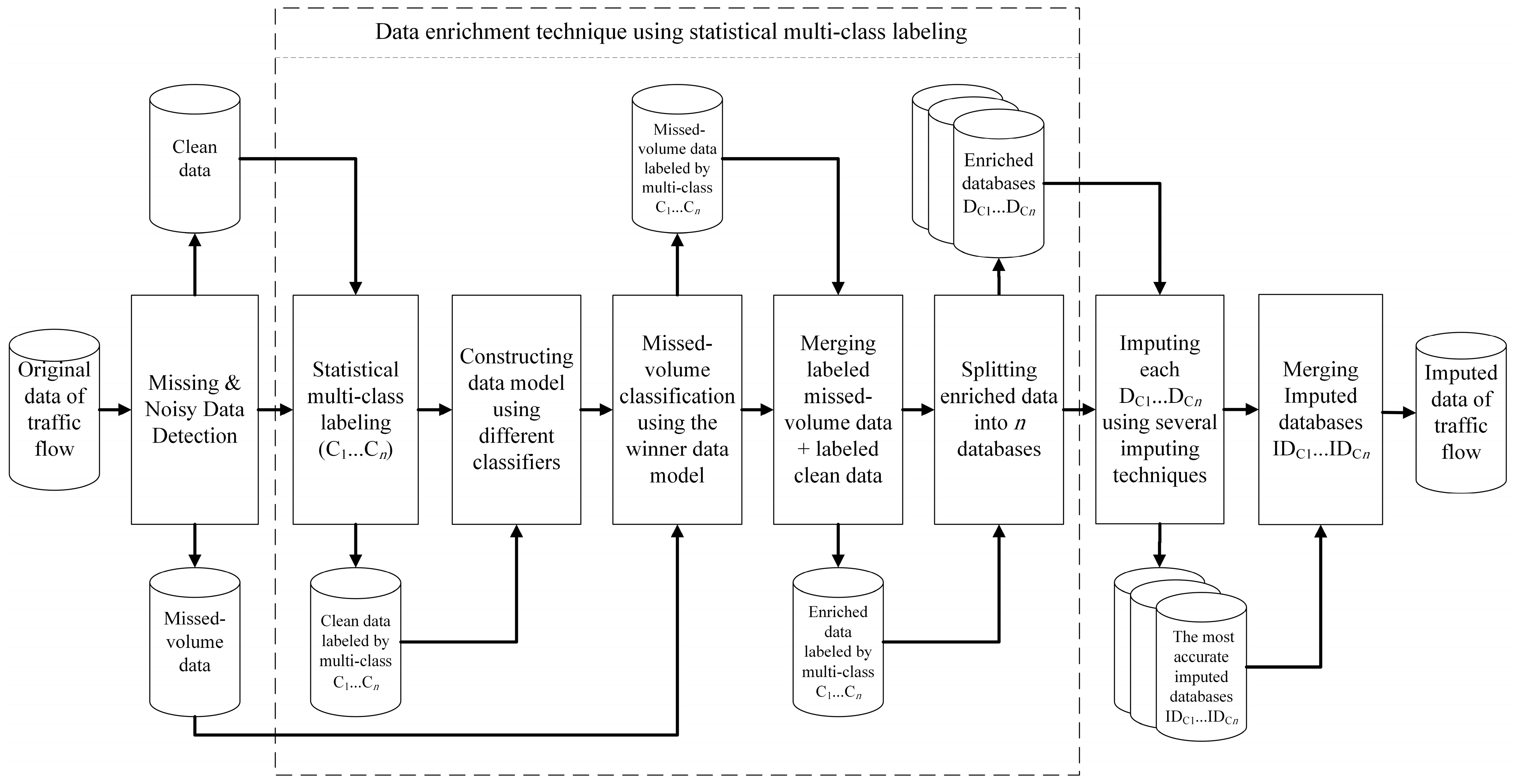
- Statistical labeling: The clean dataset formed in the previous phase is statistically labeled using multi-class C1…Cn. First, similar that of other studies [67,68], we consider five (n = 5) traffic classes named class labels consisting of very low (VL), low (L), medium (M), high (H), and very high (VH). These class labels had been determined by experts of the traffic control department in Isfahan city based on their experiences and historical traffic data.
- −
- Since smaller volume ranges provide specific subclass labels within each of the five class labels and can result in reducing the imputation error, therefore we consider the statistical labeling with subclass labels, for instance, 10 or 20 labels. It is expected that the data model constructed using the subclass labels will provide superior results compared to class labels, if the number of samples in smaller classes of the subclass labels have also sufficient samples to train the data model accurately. Table 2 shows the class labels and a subdivision the subclass labels of them including their ranges used in this study. In this table, µ and σ are the mean and the standard deviation distance.
- −
- Data Model construction: The EIM-LD method constructs data models of the clean dataset, using both class labels and subclass labels. The data models are built using k-fold and different classifiers: k-nearest neighbor (KNN), artificial neural network (ANN), Naïve Bayesian (NB), decision tree (DT), and support vector machines (SVM). The accuracy of each data model is assessed to determine the candidate data model with the highest accuracy.
- −
- Missed-volume classification: In this step, the candidate data model is used to label the samples of the missed-volume dataset to construct the labeled missed-volume dataset. The label added to the missed-volume dataset is an informative indicator which can increase the accuracy of the data model that is used in the imputation step.
- −
- Constructing the labeled dataset: In this step, the missed-volume dataset labeled in the previous step is merged with the labeled clean dataset to build the enriched data, including multi-class C1…Cn. It is expected that the imputation accuracy will be increased using this enriched data instead of using the original dataset because of adding the label to each sample.
- −
- Splitting enriched data: In this step, the enriched data are split into n enriched databases DC1 to DCn. Dividing the enriched data into n databases, each representing specific traffic classes C1…Cn, is anticipated to yield a refined data model. This approach holds the potential to construct more precise data models for split databases.
4.3. Phase 3: Imputation
- −
- Data Imputation: Missing data in databases DC1 to DCn are imputed using five commonly used methods: ARIMA, KF, BN, PPCA, and KNN, as suggested in the literature. This comprehensive approach ensures a more accurate estimation of missing data.
- −
- Merging imputed databases: Finally, the EIM-LD merges imputed databases of IDc1…IDcn by concatenating them to build the imputed data of traffic flow.
| Algorithm 1. Effective imputation method for missing volume of loop detectors (EIM-LD) | |
| Input: Original traffic flow data, n. | |
| Output: Imputed traffic flow data. | |
| 1. | Begin |
| 2. | Splitting the original data into clean and missed-volume datasets by detecting missing and noisy data using Equation (1). |
| 3. | Building the labeled clean dataset using statistical multi-class labeling C1…Cn. |
| 4. | Selecting the candidate data model constructed by several classifiers for the labeled clean dataset. |
| 5. | Determining the class of samples of the missed-volume dataset using the candidate data model. |
| 6. | Merging labeled missed-volume and labeled clean datasets to build the enriched data. |
| 7. | Splitting the enriched data into n databases DC1 to DCn. |
| 8. | For i:1 to n |
| 9. | Imputing DCi using several imputation techniques. |
| 10. | Considering imputed results with the highest accuracy as IDCi. |
| 11. | End |
| 12. | Merging imputed databases IDc1…IDcn to build ID. |
| 13. | Return ID as the imputed traffic flow data. |
| 14. | End |
5. Evaluation of the Proposed Method (EIM-LD)
5.1. Experimental Environment
5.2. Data Description
5.3. Imputation without Data Enrichment (IWDE)
5.4. EIM-LD Using Data Enrichment with Macro Classification (EMAC)
5.5. EIM-LD Using Data Enrichment with Micro Classification (EMIC)
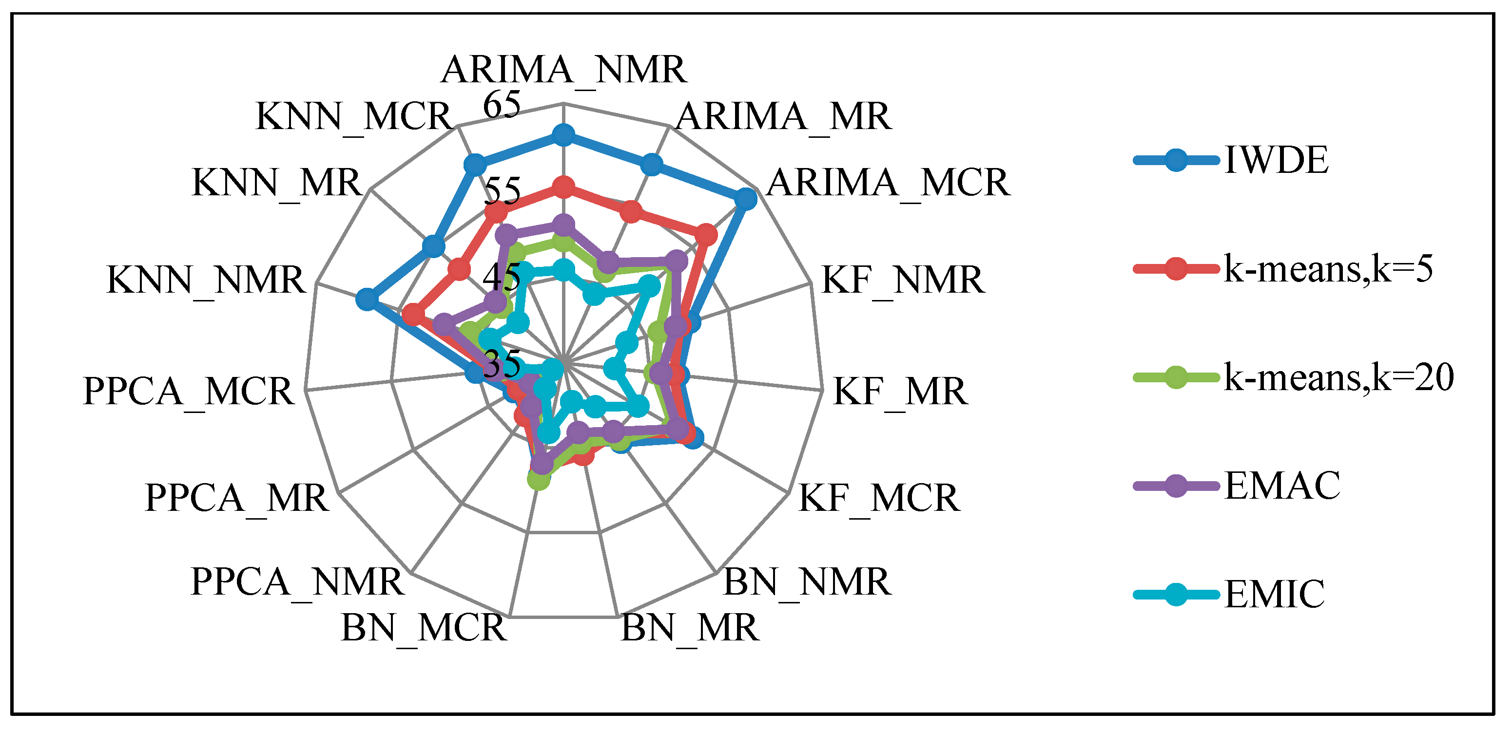
5.6. Impact Analysis of Using EIM-LD vs. Clustering
6. Discussion
7. Conclusions and Future Work
- The proposed EIM-LD method using data enrichment technique with subclass labels is superior to other comparative methods.
- The ANN classifier is more powerful than other classifiers to estimate the missing volumes of traffic flow data.
- Adding the statistical label to the original flow data can increase the training accuracy of data models in the imputing process.
Author Contributions
Funding
Data Availability Statement
Conflicts of Interest
Appendix A

Appendix B
| Classifier | Using the Original Data including Missing and Noisy Data | Using the Original Data without Missing Data | Using the Original Data without Missing and Noisy Data | Using the Enriched Data (The Labeled Clean Data Mereged with the Labeled Missed-Volume Data) |
|---|---|---|---|---|
| KNN | 50.65% | 51.83% | 71.40% | 74.80% |
| ANN | 61.45% | 62.80% | 80.48% | 81.15% |
| NB | 60.79% | 61.73% | 79.46% | 81.02% |
| DT | 56.74% | 56.67% | 76.32% | 77.89% |
| SVM | 54.03% | 56.11% | 70.64% | 72.03% |
Appendix C
| Missing Ratio | Method | Mean | Std. Deviation | Minimum | Maximum | Percentiles | ||
|---|---|---|---|---|---|---|---|---|
| 25th | 50th (Median) | 75th | ||||||
| IWDE | 51.8240 | 7.44962 | 41.59 | 63.33 | 45.1500 | 50.3300 | 60.0600 | |
| K-means, k = 5 | 49.1900 | 5.05404 | 41.00 | 57.15 | 45.1200 | 49.1200 | 54.1400 | |
| 10% | K-means, k = 20 | 45.9293 | 3.71281 | 38.10 | 52.15 | 44.4000 | 46.3200 | 48.8900 |
| EMAC | 46.7260 | 3.88193 | 39.47 | 52.58 | 43.2000 | 46.8200 | 50.1600 | |
| EMIC | 42.5687 | 3.11696 | 36.53 | 48.29 | 40.6800 | 42.7100 | 44.9200 | |
| IWDE | 54.1087 | 7.74029 | 43.51 | 65.89 | 46.7100 | 53.1500 | 62.0400 | |
| K-means, k = 5 | 51.0647 | 5.53795 | 42.19 | 60.85 | 46.0000 | 52.1300 | 56.1900 | |
| 20% | K-means, k = 20 | 47.6380 | 3.66986 | 40.05 | 54.50 | 45.6100 | 47.7300 | 50.5000 |
| EMAC | 48.4467 | 4.01378 | 40.13 | 54.34 | 45.0800 | 48.8300 | 51.7500 | |
| EMIC | 44.8327 | 3.13031 | 38.67 | 50.57 | 42.8400 | 44.8200 | 47.3200 | |
| IWDE | 56.3640 | 8.28219 | 44.91 | 69.00 | 48.1900 | 55.0300 | 65.5900 | |
| K-means, k = 5 | 53.1587 | 5.54627 | 44.00 | 62.15 | 48.0100 | 54.8200 | 58.1800 | |
| 30% | K-means, k = 20 | 49.6567 | 3.47638 | 41.73 | 55.12 | 47.9000 | 49.5900 | 52.2000 |
| EMAC | 50.6680 | 4.20448 | 42.07 | 56.70 | 47.1200 | 50.6800 | 54.2500 | |
| EMIC | 47.2673 | 3.26174 | 40.87 | 52.99 | 45.0400 | 46.9300 | 49.9700 | |
| IWDE-40% | 58.8473 | 8.20820 | 47.05 | 72.17 | 51.3200 | 58.9100 | 67.2500 | |
| K-means, k = 5 | 55.1393 | 5.67917 | 45.93 | 64.40 | 49.1200 | 56.3200 | 60.1500 | |
| 40% | K-means, k = 20 | 51.6567 | 3.48023 | 44.50 | 57.89 | 49.6000 | 51.5900 | 53.7000 |
| EMAC | 53.0293 | 4.51352 | 43.68 | 59.19 | 49.3300 | 53.0300 | 56.9100 | |
| EMIC | 49.5887 | 3.30705 | 43.27 | 55.80 | 47.2500 | 49.0900 | 51.8500 | |
| IWDE | 61.0987 | 8.94094 | 48.15 | 76.15 | 53.1500 | 60.0100 | 69.9900 | |
| K-means, k = 5 | 57.4753 | 5.72749 | 47.13 | 66.15 | 51.9000 | 58.1200 | 62.1500 | |
| 50% | K-means, k = 20 | 53.5140 | 3.31737 | 47.60 | 59.69 | 51.1800 | 53.3200 | 55.5500 |
| EMAC | 54.7087 | 4.25499 | 44.82 | 59.39 | 51.8500 | 55.3500 | 58.3300 | |
| EMIC | 51.8307 | 3.41097 | 45.37 | 58.33 | 49.7800 | 51.3500 | 54.0000 | |
References
- Allam, Z.; Dhunny, Z.A. On big data, artificial intelligence and smart cities. Cities 2019, 89, 80–91. [Google Scholar] [CrossRef]
- Saifuzzaman, M.; Moon, N.N.; Nur, F.N. IoT based street lighting and traffic management system. In Proceedings of the 2017 IEEE Region 10 Humanitarian Technology Conference (R10-HTC), Dhaka, Bangladesh, 21–23 December 2017; pp. 121–124. [Google Scholar]
- Saifuzzaman, M.; Shetu, S.F.; Moon, N.N.; Nur, F.N.; Ali, M.H. IoT based street lighting using dual axis solar tracker and effective traffic management system using deep learning: Bangladesh context. In Proceedings of the 2020 11th International Conference on Computing, Communication and Networking Technologies (ICCCNT), Kharagpur, India, 1–3 July 2020; pp. 1–5. [Google Scholar]
- Studer, L.; Ketabdari, M.; Marchionni, G. Analysis of adaptive traffic control systems design of a decision support system for better choices. J. Civ. Environ. Eng. 2015, 5, 1000195. [Google Scholar] [CrossRef]
- Sun, T.; Zhu, S.; Hao, R.; Sun, B.; Xie, J. Traffic Missing Data Imputation: A Selective Overview of Temporal Theories and Algorithms. Mathematics 2022, 10, 2544. [Google Scholar] [CrossRef]
- Nadimi-Shaharaki, M.H.; Ghahramani, M. Efficient data preparation techniques for diabetes detection. In Proceedings of the IEEE EUROCON 2015-International Conference on Computer as a Tool (EUROCON), Salamanca, Spain, 8–11 September 2015; pp. 1–6. [Google Scholar]
- World Health Organization. Regional Office for Europe: Air Quality Guidelines: Global Update 2005: Particulate Matter, Ozone, Nitrogen Dioxide, and Sulfur Dioxide; World Health Organization: Copenhagen, Denmark, 2006. [Google Scholar]
- Briedis, P.; Samuels, S. The accuracy of inductive loop detectors. In Proceedings of the ARRB Conference, 24th, 2010ARRB Group Limited, Melbourne, Australia, 12–15 October 2010. [Google Scholar]
- van Zuylen, H. Loop Detector Error and Its Impacts on Traffic Control Scheme. 2010. Available online: https://rstrail.nl/wp-content/uploads/2015/02/Jie_Li.pdf (accessed on 20 January 2023).
- Ma, X.; Luan, S.; Du, B.; Yu, B. Spatial copula model for imputing traffic flow data from remote microwave sensors. Sensors 2017, 17, 2160. [Google Scholar] [CrossRef] [PubMed]
- Liu, H.; Li, L. Missing Data Imputation in GNSS Monitoring Time Series Using Temporal and Spatial Hankel Matrix Factorization. Remote Sens. 2022, 14, 1500. [Google Scholar] [CrossRef]
- Qu, L.; Li, L.; Zhang, Y.; Hu, J. PPCA-based missing data imputation for traffic flow volume: A systematical approach. IEEE Trans. Intell. Transp. Syst. 2009, 10, 512–522. [Google Scholar]
- Chen, H.; Grant-Muller, S.; Mussone, L.; Montgomery, F. A study of hybrid neural network approaches and the effects of missing data on traffic forecasting. Neural Comput. Appl. 2001, 10, 277–286. [Google Scholar] [CrossRef]
- Liu, Z.; Sharma, S.; Datla, S. Imputation of missing traffic data during holiday periods. Transp. Plan. Technol. 2008, 31, 525–544. [Google Scholar] [CrossRef]
- Redfern, E.; Watson, S.; Clark, S.; Tight, M.; Payne, G. Modelling Outliers and Missing Values in traffic Count Data Using the ARIMA Model; Institute of Transport Studies, University of Leeds: Leeds, UK, 1993. [Google Scholar]
- Van Lint, J.; Hoogendoorn, S.; van Zuylen, H.J. Accurate freeway travel time prediction with state-space neural networks under missing data. Transp. Res. Part C Emerg. Technol. 2005, 13, 347–369. [Google Scholar] [CrossRef]
- Zhong, M.; Sharma, S.; Lingras, P. Genetically designed models for accurate imputation of missing traffic counts. Transp. Res. Rec. 2004, 1879, 71–79. [Google Scholar] [CrossRef]
- Ni, D.; Leonard, J.D.; Guin, A.; Feng, C. Multiple imputation scheme for overcoming the missing values and variability issues in ITS data. J. Transp. Eng. 2005, 131, 931–938. [Google Scholar] [CrossRef]
- Ni, D.; Leonard, J.D. Markov chain monte carlo multiple imputation using bayesian networks for incomplete intelligent transportation systems data. Transp. Res. Rec. 2005, 1935, 57–67. [Google Scholar] [CrossRef]
- Sun, B.; Cheng, W.; Goswami, P.; Bai, G. Short-term traffic forecasting using self-adjusting k-nearest neighbours. IET Intell. Transp. Syst. 2017, 12, 41–48. [Google Scholar] [CrossRef]
- Xu, D.-W.; Wang, Y.-D.; Jia, L.-M.; Li, H.-J.; Zhang, G.-J. Real-time road traffic states measurement based on Kernel-KNN matching of regional traffic attractors. Measurement 2016, 94, 862–872. [Google Scholar] [CrossRef]
- Jia, X.; Dong, X.; Chen, M.; Yu, X. Missing data imputation for traffic congestion data based on joint matrix factorization. Knowl.-Based Syst. 2021, 225, 107114. [Google Scholar] [CrossRef]
- Chen, X.; Wei, Z.; Li, Z.; Liang, J.; Cai, Y.; Zhang, B. Ensemble correlation-based low-rank matrix completion with applications to traffic data imputation. Knowl.-Based Syst. 2017, 132, 249–262. [Google Scholar] [CrossRef]
- Gang, C.; Qiaoyun, W.; Lei, L. Missing data imputataion for traffic flow based on weighted local least squares. In Proceedings of the International Conference on Automatic Control and Artificial Intelligence (ACAI 2012), Xiamen, China, 3–5 March 2012. [Google Scholar]
- Chang, G.; Zhang, Y.; Yao, D. Missing data imputation for traffic flow based on improved local least squares. Tsinghua Sci. Technol. 2012, 17, 304–309. [Google Scholar] [CrossRef]
- Nguyen, L.N.; Scherer, W.T. Imputation Techniques to Account for Missing Data in Support of Intelligent Transportation Systems Applications; Citeseer: Princeton, NJ, USA, 2003. [Google Scholar]
- Haworth, J.; Cheng, T. Non-parametric regression for space–time forecasting under missing data. Comput. Environ. Urban Syst. 2012, 36, 538–550. [Google Scholar] [CrossRef]
- Li, L.; Li, Y.; Li, Z. Efficient missing data imputing for traffic flow by considering temporal and spatial dependence. Transp. Res. Part C Emerg. Technol. 2013, 34, 108–120. [Google Scholar] [CrossRef]
- Tan, H.; Feng, G.; Feng, J.; Wang, W.; Zhang, Y.-J.; Li, F. A tensor-based method for missing traffic data completion. Transp. Res. Part C Emerg. Technol. 2013, 28, 15–27. [Google Scholar] [CrossRef]
- Chen, C.; Kwon, J.; Rice, J.; Skabardonis, A.; Varaiya, P. Detecting errors and imputing missing data for single-loop surveillance systems. Transp. Res. Rec. J. Transp. Res. Board 2003, 1855, 160–167. [Google Scholar] [CrossRef]
- Henrickson, K.; Zou, Y.; Wang, Y. Flexible and robust method for missing loop detector data imputation. Transp. Res. Rec. 2015, 2527, 29–36. [Google Scholar] [CrossRef]
- Tak, S.; Woo, S.; Yeo, H. Data-Driven Imputation Method for Traffic Data in Sectional Units of Road Links. IEEE Trans. Intell. Transp. Syst. 2016, 17, 1762–1771. [Google Scholar] [CrossRef]
- Smith, B.L.; Scherer, W.T.; Conklin, J.H. Exploring imputation techniques for missing data in transportation management systems. Transp. Res. Rec. 2003, 1836, 132–142. [Google Scholar] [CrossRef]
- Tang, J.; Wang, Y.; Zhang, S.; Wang, H.; Liu, F.; Yu, S. On Missing Traffic Data Imputation Based on Fuzzy C-Means Method by Considering Spatial–Temporal Correlation. Transp. Res. Rec. J. Transp. Res. Board 2015, 2528, 86–95. [Google Scholar] [CrossRef]
- Ahmed, M.S.; Cook, A.R. Analysis of Freeway Traffic Time-Series Data by Using Box-Jenkins Techniques; Transportation Research Board: Washington, DC, USA, 1979. [Google Scholar]
- Karlaftis, M.G.; Vlahogianni, E.I. Statistical methods versus neural networks in transportation research: Differences, similarities and some insights. Transp. Res. Part C Emerg. Technol. 2011, 19, 387–399. [Google Scholar] [CrossRef]
- Vlahogianni, E.I.; Karlaftis, M.G.; Golias, J.C. Optimized and meta-optimized neural networks for short-term traffic flow prediction: A genetic approach. Transp. Res. Part C Emerg. Technol. 2005, 13, 211–234. [Google Scholar] [CrossRef]
- Zhang, T.; Zhang, D.-g.; Yan, H.-r.; Qiu, J.-n.; Gao, J.-x. A new method of data missing estimation with FNN-based tensor heterogeneous ensemble learning for internet of vehicle. Neurocomputing 2021, 420, 98–110. [Google Scholar] [CrossRef]
- Castro-Neto, M.; Jeong, Y.-S.; Jeong, M.-K.; Han, L.D. Online-SVR for short-term traffic flow prediction under typical and atypical traffic conditions. Expert Syst. Appl. 2009, 36, 6164–6173. [Google Scholar] [CrossRef]
- Jin, X.; Zhang, Y.; Yao, D. Simultaneously prediction of network traffic flow based on PCA-SVR. In Proceedings of the International Symposium on Neural Networks, Nanjing, China, 3–7 June 2007; pp. 1022–1031. [Google Scholar]
- Zhang, C.; Sun, S.; Yu, G. A Bayesian network approach to time series forecasting of short-term traffic flows. In Proceedings of the 7th International IEEE Conference on Intelligent Transportation Systems (IEEE Cat. No. 04TH8749), Washington, WA, USA, 3–6 October 2004; pp. 216–221. [Google Scholar]
- Ghosh, B.; Basu, B.; O’Mahony, M. Bayesian time-series model for short-term traffic flow forecasting. J. Transp. Eng. 2007, 133, 180–189. [Google Scholar] [CrossRef]
- Vlahogianni, E.I.; Golias, J.C.; Karlaftis, M.G. Short-term traffic forecasting: Overview of objectives and methods. Transp. Rev. 2004, 24, 533–557. [Google Scholar] [CrossRef]
- Tekler, Z.D.; Ono, E.; Peng, Y.; Zhan, S.; Lasternas, B.; Chong, A. ROBOD, room-level occupancy and building operation dataset. In Building Simulation; Tsinghua University Press: Beijing, China, 2022; pp. 2127–2137. [Google Scholar]
- Li, J.; Van Zuylen, H.J.; Wei, G. Loop detector data error diagnosing and interpolating with probe vehicle data. In Proceedings of the 93rd Annual Meeting Transportation Research Board, Washington, WA, USA, 12–16 January 2014. Authors version. [Google Scholar]
- Chen, C.; Wang, Y.; Li, L.; Hu, J.; Zhang, Z. The retrieval of intra-day trend and its influence on traffic prediction. Transp. Res. Part C Emerg. Technol. 2012, 22, 103–118. [Google Scholar] [CrossRef]
- Li, Y.; Li, Z.; Li, L.; Zhang, Y.; Jin, M. Comparison on PPCA, KPPCA and MPPCA based missing data imputing for traffic flow. In ICTIS 2013: Improving Multimodal Transportation Systems-Information, Safety, and Integration; American Society of Civil Engineers: Reston, VA, USA, 2013; pp. 1151–1156. [Google Scholar]
- Qu, L.; Zhang, Y.; Hu, J.; Jia, L.; Li, L. A BPCA based missing value imputing method for traffic flow volume data. In Proceedings of the 2008 IEEE Intelligent Vehicles Symposium, Eindhoven, The Netherlands, 4–6 June 2008; pp. 985–990. [Google Scholar]
- Goves, C.; North, R.; Johnston, R.; Fletcher, G. Short term traffic prediction on the UK motorway network using neural networks. Transp. Res. Procedia 2016, 13, 184–195. [Google Scholar] [CrossRef]
- Li, Y.; Li, Z.; Li, L. Missing traffic data: Comparison of imputation methods. IET Intell. Transp. Syst. 2014, 8, 51–57. [Google Scholar] [CrossRef]
- Stekhoven, D.J.; Bühlmann, P. MissForest—non-parametric missing value imputation for mixed-type data. Bioinformatics 2012, 28, 112–118. [Google Scholar] [CrossRef] [PubMed]
- Yoon, J.; Jordon, J.; Schaar, M. Gain: Missing data imputation using generative adversarial nets. In Proceedings of the 35th International Conference on Machine Learning, Stockholm, Sweden, 10–15 July 2018; pp. 5689–5698. Available online: https://www.vanderschaar-lab.com/papers/ICML_GAIN.pdf (accessed on 25 January 2023).
- Low, R.; Tekler, Z.D.; Cheah, L. Predicting commercial vehicle parking duration using generative adversarial multiple imputation networks. Transp. Res. Rec. 2020, 2674, 820–831. [Google Scholar] [CrossRef]
- Yin, W.; Murray-Tuite, P.; Rakha, H. Imputing erroneous data of single-station loop detectors for nonincident conditions: Comparison between temporal and spatial methods. J. Intell. Transp. Syst. 2012, 16, 159–176. [Google Scholar] [CrossRef]
- Zhong, M.; Sharma, S.; Liu, Z. Assessing robustness of imputation models based on data from different jurisdictions: Examples of Alberta and Saskatchewan, Canada. Transp. Res. Rec. 2005, 1917, 116–126. [Google Scholar] [CrossRef]
- Williams, B.M. Multivariate vehicular traffic flow prediction: Evaluation of ARIMAX modeling. Transp. Res. Rec. 2001, 1776, 194–200. [Google Scholar] [CrossRef]
- Weijermars, W.; Van Berkum, E. Detection of invalid loop detector data in urban areas. Transp. Res. Rec. J. Transp. Res. Board 2006, 1945, 82–88. [Google Scholar] [CrossRef]
- Lu, X.-Y.; Kim, Z.; Cao, M.; Guo, Z.; Johnston, S.; Spring, J.; Varaiya, P.P.; Horowitz, R. Deliver a Set of Tools for Resolving Bad Inductive Loops and Correcting Bad Data; California PATH, ITS, University of California, Berkeley: Berkeley, CA, USA, 2012. [Google Scholar]
- Xiao, X.; Chen, Y.; Yuan, Y. Estimation of missing flow at junctions using control plan and floating car data. Transp. Res. Procedia 2015, 10, 113–123. [Google Scholar] [CrossRef]
- Bae, B.; Kim, H.; Lim, H.; Liu, Y.; Han, L.D.; Freeze, P.B. Missing data imputation for traffic flow speed using spatio-temporal cokriging. Transp. Res. Part C Emerg. Technol. 2018, 88, 124–139. [Google Scholar] [CrossRef]
- Administration, F.H. Traffic Detector Handbook. FHWA 2006, I, 4–49. [Google Scholar]
- Hox, J.J. A review of current software for handling missing data. Kwant. Methoden 1999, 20, 123–138. [Google Scholar]
- Barnett, V.; Lewis, T. Outliers in Statistical Data; John Wiley and Sons: New York, NY, USA, 1994. [Google Scholar]
- Zhao, N.; Li, Z.; Li, Y. Improving the traffic data imputation accuracy using temporal and spatial information. In Proceedings of the 2014 7th International Conference on Intelligent Computation Technology and Automation, Changsha, China, 25–26 October 2014; pp. 312–317. [Google Scholar]
- Nadimi-Shahraki, M.H.; Mohammadi, S.; Zamani, H.; Gandomi, M.; Gandomi, A.H. A hybrid imputation method for multi-pattern missing data: A case study on type II diabetes diagnosis. Electronics 2021, 10, 3167. [Google Scholar] [CrossRef]
- Saw, J.G.; Yang, M.C.; Mo, T.C. Chebyshev inequality with estimated mean and variance. Am. Stat. 1984, 38, 130–132. [Google Scholar]
- Christantonis, K.; Tjortjis, C.; Manos, A.; Filippidou, D.E.; Mougiakou, Ε.; Christelis, E. Using classification for traffic prediction in smart cities. In Proceedings of the Artificial Intelligence Applications and Innovations: 16th IFIP WG 12.5 International Conference, AIAI 2020, Neos Marmaras, Greece, 5–7 June 2020; pp. 52–61. [Google Scholar]
- Pasindu, H.; Gamage, D.; Bandara, J. Framework for selecting pavement type for low volume roads. Transp. Res. Procedia 2020, 48, 3924–3938. [Google Scholar] [CrossRef]
- Nadimi-Shahraki, M.H.; Fatahi, A.; Zamani, H.; Mirjalili, S. Binary Approaches of Quantum-Based Avian Navigation Optimizer to Select Effective Features from High-Dimensional Medical Data. Mathematics 2022, 10, 2770. [Google Scholar] [CrossRef]
- Nadimi-Shahraki, M.H.; Zamani, H.; Fatahi, A.; Mirjalili, S. MFO-SFR: An enhanced moth-flame optimization algorithm using an effective stagnation finding and replacing strategy. Mathematics 2023, 11, 862. [Google Scholar] [CrossRef]




| Ref | Method Used for IMPUTING | Volume of Data | Volume of Missing Data | Advantages | Disadvantages |
|---|---|---|---|---|---|
| Tekler et al. [44] | Random Forest-based imputation algorithm | 52,128 | 2684 | The ROBOD dataset helps building managers save energy, reduce waste, and cut expenses by providing detailed usage and operation information. | Room-level occupancy and building operation data are the only focus of the ROBOD data set. Sensor location, adjustment, and upkeep can affect data reliability, resulting in potentially incorrect or incomplete results. |
| Briedis et al. [8] | Comparison of field statistics with statistics obtained from SCATS system Using statistical methods and graphing. | 800 | - | Analyzing the inductive detector’s performance involves comparing field results with SCATS and assessing factors such as lane count, traffic type, asphalt condition, vehicle volume, and movement mode. | The simultaneous effect of two factors on the inductive detector accuracy and the lack of its examination. |
| Li et al. [45] | Comparison of field data with system data-error detection algorithm | 408,960 | - | 25% of the tested inductive detectors had an error over 20%. This method measures vehicle flow, monitors queue length, and estimates GPS-equipped vehicles. | The routes need to be reconstructed to reduce the driver’s disorder, which improves the accuracy of the flow estimation on the route. |
| Li et al. [50] | Prediction methods, interpolation methods and statistical learning methods | 12,384 | - | PPCA yields best performance in all aspects and numerical tests demonstrate that it can be used to impute data online before making further and is robust to weather changes. | From a statistical perspective, prediction and MCMC methods are not advisable. |
| Stekhoven et al. [51] | Iterative imputation method (MissForest) based on a random forest algorithm | 10 datasets | 10, 20 or 30% | Miss-Forest is a reliable method for imputing high proportions of missing data in large datasets with many variables and observations. It generates multiple imputations, enabling consideration of imputation uncertainty in subsequent analyses. | Limitations for dealing with some kinds of mixed data. Imputed values from MissForest can be distorted with varying missing data patterns. The quality of imputed values in MissForest depends on parameters such as tree number and convergence criterion, making optimal settings challenging to determine. |
| Yoon et al. [52] | A machine learning technique for imputing missing data using Generative Adversarial Nets (GANs) | 5 datasets | - | The GAIN method utilizes GANs to accurately impute missing data, handles diverse data types (continuous, categorical, mixed), and is robust against outliers and noise, making it suitable for real-world datasets. | GAIN requires ample data for effective GAN training and may struggle with complex data, resulting in inaccurate imputations. Training GAN is time-consuming, a drawback for time-sensitive data. Biased training or inadequate model adjustments in GAIN may introduce bias in imputed data. |
| Low et al. [53] | Missing data imputation using generative adversarial multiple imputation algorithm | - | 0.000 to 0.980 | Develop a regression model to predict the parking duration of commercial vehicles at the loading bays of retail malls and identify significant factors that contribute to this dwell time. | Training GANs is expensive and time-consuming. GAMIN can overfit, leading to poor generalization on new datasets. |
| Chen et al. [30] | DSA algorithm for error detection–linear regression algorithm | 42 million sample | 15% | By applying the linear regression algorithm, it can estimate the missing data more accurately than using historical data. This way, all the sensors that have a good neighbor will have their data completed in after running the algorithm once. | Linear regression fills most of the fields in the first run, but the accuracy of the filled fields decreases with each subsequent run. |
| Weijermars et al. [57] | Data quality check method to identify invalid data generated by inductive detector and Macroscopic quality checks Microscopic | 3000 | 3.4% | Minimum and maximum flow thresholds are used to detect erroneous data. Macroscopic quality checks are a useful addition to the microscopic quality checks. | Microscopic data quality check does not detect many erroneous data. Flows are inconsistent between upstream detectors mutually in some cases, it is not always clear whether the results of this quality check are reliable. |
| Liu et al. [14] | Non-Parametric regression-the K-NN method | 25,200 | - | The proper performance of K-NN method in correcting lost data during holidays. | The ARIMA model fails to work properly when the traffic conditions vary across seasons. |
| Lu et al. [58] | Spatial and Temporal Correlation | 2880 | - | This method works well for highways or intersections where we can get the upstream and downstream volume or estimate the error by comparing the camera data and the hardware data. | Analyzing aggregated data at the macroscopic level is not an effective method for fault detection. This approach fails for intersections that lack data from both upstream and downstream sources. |
| Tang et al. [34] | Fuzzy C-means(FCM) | 77,760 | 25,920 | This research analyzes the data for weekdays and weekends separately, which improves the accuracy of measuring the methods’ efficiency. | NMR, MCR data patterns are not used. |
| Xiao et al. [59] | Historical Pattern- Timing Plan- FCD | 3744 | - | The methods show reliable results after several iterations. | In different conditions and approaches, the desired results and efficiency may not be achieved. |
| Tak et al. [32] | Data Driven method based on Spatial and Temporal Correlation using a modified knn method | 135,936 | - | The health vector enables the optimal computation of the Euclidean distance between the historical and subject data. KNN performance does not differ for weekday and weekend data. | B-EM is more effective for single identifier data than multiple neighboring identifiers. NH performance varies based on weekdays or weekends. |
| Bae et al. [60] | Cokriging method- spatial–temporal | 8064 | 1113 | The SK and OK methods excel on the MCAR data pattern. The SCK method is effective on the MNAR data pattern. | The OCK method results may become less accurate if there is no data from neighboring. |
| Row | Range | Class Labels | Volume | Subclass Labels | Sub-Volume |
|---|---|---|---|---|---|
| 1 | [0, (µ − 1.5σ)) | Very Low (VL) | 0–19 | VL1 | 0–4 |
| VL2 | 5–9 | ||||
| VL3 | 10–14 | ||||
| VL4 | 15–19 | ||||
| 2 | [(µ − 1.5σ), (µ − 1/2σ)) | Low (L) | 20–48 | L1 | 20–27 |
| L2 | 28–34 | ||||
| L3 | 35–41 | ||||
| L4 | 42–48 | ||||
| 3 | [(µ − 1/2σ), (µ + 1.5σ)) | Medium (M) | 49–105 | M1 | 49–63 |
| M2 | 64–77 | ||||
| M3 | 78–91 | ||||
| M4 | 92–105 | ||||
| 4 | [(µ + 1.5σ), (µ + 3σ)) | High (H) | 106–147 | H1 | 106–115 |
| H2 | 116–126 | ||||
| H3 | 127–137 | ||||
| H4 | 138–147 | ||||
| 5 | [(µ + 3σ), max] | Very High (VH) | 148 to (max) | VH1 | 148–173 |
| VH2 | 174–198 | ||||
| VH3 | 199–223 | ||||
| VH4 | 224–max |
| Feature | Info. Gain | Gain Ratio | Gini |
|---|---|---|---|
| Time | 0.381 | 0.058 | 0.094 |
| Month | 0.158 | 0.044 | 0.027 |
| Season | 0.098 | 0.049 | 0.016 |
| Weekday | 0.004 | 0.001 | 0.001 |
| Date | 0.003 | 0.002 | 0.001 |
| Holiday | 0.002 | 0.003 | 0.001 |
| Rainy | 0.001 | 0.002 | 0.000 |
| K | Outlier (n) | Outlier (%) | Acc. KNN | Acc. ANN | Acc. NB | Acc. DT | Acc. SVM |
|---|---|---|---|---|---|---|---|
| 1 | 3864 | 14.097 | 71.40% | 80.48% | 79.46% | 78.32% | 70.64% |
| sqrt(2) | 2221 | 8.103 | 68.84% | 75.84% | 75.59% | 72.72% | 68.19% |
| 1.5 | 2028 | 7.399 | 68.30% | 75.36% | 75.17% | 72.46% | 68.10% |
| 2 | 1230 | 4.488 | 66.30% | 73.74% | 73.51% | 70.65% | 66.83% |
| 3 | 639 | 2.332 | 65.24% | 72.99% | 72.32% | 69.32% | 65.52% |
| 4 | 388 | 1.416 | 64.67% | 72.35% | 71.71% | 68.94% | 64.96% |
| 5 | 251 | 0.916 | 64.31% | 72.54% | 71.50% | 68.56% | 64.54% |
| 6 | 148 | 0.54 | 64.22% | 72.28% | 71.42% | 68.42% | 64.41% |
| 7 | 105 | 0.384 | 64.08% | 72.04% | 71.38% | 68.35% | 64.37% |
| 8 | 90 | 0.329 | 64.08% | 71.75% | 71.36% | 68.35% | 64.41% |
| 9 | 77 | 0.281 | 64.06% | 72.20% | 71.32% | 68.33% | 63.92% |
| 10 | 70 | 0.256 | 64.06% | 71.83% | 71.31% | 68.14% | 64.39% |
| Missing Ratio | ARIMA | KF | BN | PPCA | KNN | ||||||||||
|---|---|---|---|---|---|---|---|---|---|---|---|---|---|---|---|
| NMR | MR | MCR | NMR | MR | MCR | NMR | MR | MCR | NMR | MR | MCR | NMR | MR | MCR | |
| 10% | 61.33 | 60.07 | 63.33 | 50.33 | 48.32 | 52.23 | 46.32 | 44.10 | 48.32 | 42.23 | 41.59 | 45.15 | 58.83 | 55.15 | 60.06 |
| 20% | 64.19 | 63.65 | 65.89 | 53.15 | 51.32 | 53.91 | 47.50 | 45.81 | 51.03 | 44.51 | 43.51 | 46.71 | 60.32 | 58.09 | 62.04 |
| 30% | 67.32 | 65.59 | 69.00 | 55.55 | 54.00 | 55.03 | 49.17 | 47.32 | 52.51 | 47.03 | 44.91 | 48.19 | 63.23 | 61.02 | 65.59 |
| 40% | 69.04 | 67.25 | 72.17 | 58.91 | 56.61 | 59.17 | 52.02 | 50.00 | 54.05 | 48.92 | 47.05 | 51.32 | 65.00 | 62.88 | 68.32 |
| 50% | 73.15 | 71.10 | 76.15 | 60.01 | 58.17 | 61.39 | 54.15 | 52.15 | 56.17 | 50.17 | 48.15 | 53.15 | 67.19 | 65.39 | 69.99 |
| Missing Ratio | ARIMA | KF | BN | PPCA | KNN | ||||||||||
|---|---|---|---|---|---|---|---|---|---|---|---|---|---|---|---|
| NMR | MR | MCR | NMR | MR | MCR | NMR | MR | MCR | NMR | MR | MCR | NMR | MR | MCR | |
| 10% | 50.95 | 47.73 | 52.58 | 48.59 | 46.29 | 50.16 | 44.77 | 43.20 | 46.82 | 41.22 | 39.47 | 42.89 | 49.48 | 45.59 | 51.15 |
| 20% | 52.60 | 49.43 | 54.34 | 50.05 | 48.42 | 51.75 | 46.52 | 45.08 | 48.83 | 42.64 | 40.13 | 44.76 | 51.18 | 48.07 | 52.90 |
| 30% | 55.25 | 52.11 | 56.70 | 52.44 | 50.47 | 54.25 | 48.65 | 47.12 | 50.68 | 44.45 | 42.07 | 46.73 | 53.72 | 50.48 | 54.90 |
| 40% | 57.33 | 54.57 | 59.03 | 54.48 | 52.98 | 59.19 | 51.47 | 49.33 | 53.03 | 46.33 | 43.68 | 48.76 | 55.58 | 52.77 | 56.91 |
| 50% | 58.94 | 57.26 | 59.22 | 56.21 | 54.61 | 58.33 | 53.07 | 51.19 | 55.35 | 48.27 | 44.82 | 51.85 | 57.62 | 54.50 | 59.39 |
| Micro Class | ARIMA | KF | BN | PPCA | KNN | ||||||||||
|---|---|---|---|---|---|---|---|---|---|---|---|---|---|---|---|
| NMR | MR | MCR | NMR | MR | MCR | NMR | MR | MCR | NMR | MR | MCR | NMR | MR | MCR | |
| VL1 | 47.38 | 45.15 | 49.79 | 44.17 | 43.47 | 46.38 | 43.83 | 41.74 | 46.36 | 42.50 | 39.47 | 44.49 | 45.92 | 44.17 | 47.54 |
| VL2 | 46.11 | 44.68 | 49.57 | 44.81 | 43.28 | 46.88 | 44.34 | 41.43 | 46.90 | 42.97 | 39.85 | 44.75 | 46.65 | 44.65 | 47.40 |
| VL3 | 47.18 | 44.73 | 49.18 | 44.50 | 43.59 | 46.44 | 44.45 | 42.77 | 40.25 | 42.70 | 40.08 | 43.90 | 47.10 | 44.40 | 48.10 |
| VL4 | 47.63 | 44.80 | 50.92 | 45.54 | 43.59 | 48.14 | 44.94 | 43.37 | 46.79 | 43.25 | 41.18 | 45.56 | 46.89 | 44.41 | 48.79 |
| L1 | 48.59 | 47.03 | 51.56 | 44.91 | 43.91 | 47.28 | 44.39 | 41.42 | 46.93 | 41.40 | 39.22 | 43.70 | 46.20 | 43.35 | 49.31 |
| L2 | 48.98 | 47.53 | 51.00 | 44.38 | 42.37 | 48.08 | 44.14 | 42.26 | 46.15 | 41.57 | 39.16 | 43.99 | 46.59 | 44.38 | 49.30 |
| L3 | 49.58 | 46.12 | 51.76 | 46.00 | 44.51 | 48.40 | 44.22 | 42.92 | 46.78 | 41.35 | 38.24 | 42.88 | 47.30 | 44.39 | 49.57 |
| L4 | 48.38 | 46.76 | 51.84 | 45.12 | 43.48 | 48.59 | 42.62 | 41.50 | 45.01 | 40.80 | 38.30 | 42.79 | 46.64 | 44.13 | 49.94 |
| M1 | 51.92 | 50.21 | 53.64 | 47.61 | 46.17 | 50.60 | 46.89 | 45.14 | 49.82 | 44.31 | 42.42 | 45.74 | 49.61 | 46.58 | 52.67 |
| M2 | 52.63 | 49.24 | 54.30 | 50.24 | 48.58 | 52.03 | 48.00 | 46.79 | 50.51 | 43.77 | 41.60 | 46.28 | 50.90 | 49.92 | 53.94 |
| M3 | 52.10 | 49.97 | 54.79 | 48.75 | 46.56 | 51.04 | 48.14 | 45.80 | 50.44 | 45.49 | 42.76 | 46.99 | 49.67 | 47.73 | 52.46 |
| M4 | 51.62 | 49.25 | 54.80 | 48.87 | 45.34 | 49.50 | 46.57 | 45.66 | 48.88 | 43.69 | 41.06 | 46.95 | 49.32 | 46.91 | 52.07 |
| H1 | 50.99 | 48.89 | 54.24 | 48.76 | 46.30 | 51.20 | 37.01 | 45.34 | 49.94 | 43.88 | 41.93 | 46.53 | 49.15 | 47.86 | 52.05 |
| H2 | 51.28 | 49.64 | 53.99 | 48.49 | 46.11 | 51.45 | 47.49 | 45.39 | 49.03 | 44.23 | 41.63 | 47.78 | 49.09 | 47.07 | 51.66 |
| H3 | 52.50 | 50.40 | 55.62 | 47.48 | 45.51 | 50.31 | 45.96 | 44.50 | 49.04 | 44.13 | 41.42 | 46.02 | 50.20 | 48.72 | 52.72 |
| H4 | 53.94 | 50.90 | 56.35 | 48.75 | 46.95 | 52.04 | 47.95 | 45.78 | 50.71 | 43.92 | 40.93 | 46.81 | 51.92 | 49.67 | 54.86 |
| VH1 | 52.82 | 52.57 | 55.02 | 47.46 | 44.77 | 50.69 | 46.14 | 44.95 | 47.06 | 42.91 | 40.79 | 45.09 | 49.77 | 46.86 | 51.95 |
| VH2 | 52.83 | 50.50 | 55.39 | 47.75 | 46.22 | 49.82 | 46.16 | 42.95 | 47.78 | 44.44 | 43.04 | 46.33 | 51.02 | 48.45 | 53.27 |
| VH3 | 51.68 | 49.55 | 55.01 | 48.48 | 45.56 | 51.22 | 46.87 | 45.15 | 48.60 | 43.37 | 42.14 | 46.52 | 50.10 | 48.19 | 52.94 |
| VH4 | 52.65 | 49.94 | 55.21 | 49.16 | 47.19 | 52.15 | 48.82 | 46.16 | 51.06 | 45.99 | 43.66 | 48.14 | 50.98 | 49.03 | 54.46 |
| Missing Ratio | ARIMA | KF | BN | PPCA | KNN | ||||||||||
|---|---|---|---|---|---|---|---|---|---|---|---|---|---|---|---|
| NMR | MR | MCR | NMR | MR | MCR | NMR | MR | MCR | NMR | MR | MCR | NMR | MR | MCR | |
| 10% | 45.75 | 43.70 | 48.29 | 42.71 | 40.95 | 44.92 | 41.23 | 39.55 | 43.18 | 38.64 | 36.53 | 40.68 | 43.91 | 42.06 | 46.43 |
| 20% | 48.01 | 45.59 | 50.57 | 44.82 | 42.84 | 47.32 | 43.57 | 41.80 | 45.78 | 41.22 | 38.67 | 43.35 | 46.12 | 43.98 | 48.85 |
| 30% | 50.34 | 48.50 | 52.99 | 46.93 | 45.04 | 49.97 | 46.04 | 44.08 | 48.59 | 43.31 | 40.87 | 45.90 | 48.49 | 46.37 | 51.59 |
| 40% | 53.04 | 50.74 | 55.80 | 49.09 | 47.25 | 51.85 | 48.42 | 46.29 | 50.75 | 45.65 | 43.27 | 47.91 | 51.30 | 48.97 | 53.50 |
| 50% | 55.56 | 53.44 | 58.33 | 51.75 | 49.78 | 54.00 | 50.50 | 48.52 | 51.22 | 47.85 | 45.37 | 49.97 | 53.94 | 51.35 | 55.88 |
| Method | Missing Ratio | ARIMA | KF | BN | PPCA | KNN | ||||||||||
|---|---|---|---|---|---|---|---|---|---|---|---|---|---|---|---|---|
| NMR | MR | MCR | NMR | MR | MCR | NMR | MR | MCR | NMR | MR | MCR | NMR | MR | MCR | ||
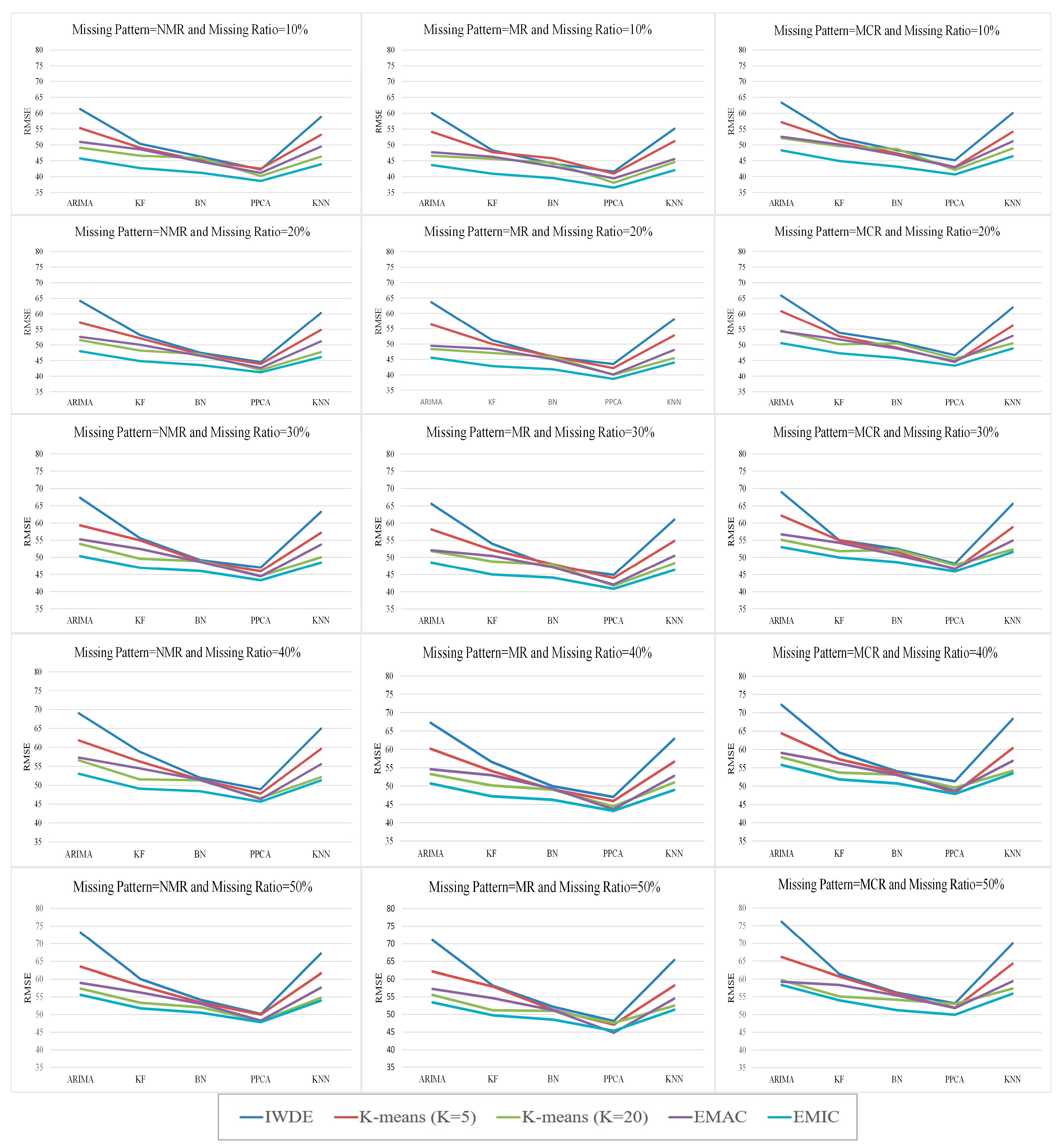
| IWDE | 10% | 61.33 | 60.07 | 63.33 | 50.33 | 48.32 | 52.23 | 46.32 | 44.10 | 48.32 | 42.23 | 41.59 | 45.15 | 58.83 | 55.15 | 60.06 |
| 20% | 64.19 | 63.65 | 65.89 | 53.15 | 51.32 | 53.91 | 47.50 | 45.81 | 51.03 | 44.51 | 43.51 | 46.71 | 60.32 | 58.09 | 62.04 | |
| 30% | 67.32 | 65.59 | 69.00 | 55.55 | 54.00 | 55.03 | 49.17 | 47.32 | 52.51 | 47.03 | 44.91 | 48.19 | 63.23 | 61.02 | 65.59 | |
| 40% | 69.04 | 67.25 | 72.17 | 58.91 | 56.61 | 59.17 | 52.02 | 50.00 | 54.05 | 48.92 | 47.05 | 51.32 | 65.00 | 62.88 | 68.32 | |
| 50% | 73.15 | 71.10 | 76.15 | 60.01 | 58.17 | 61.39 | 54.15 | 52.15 | 56.17 | 50.17 | 48.15 | 53.15 | 67.19 | 65.39 | 69.99 | |
| K-means K = 5 | 10% | 55.32 | 54.14 | 57.15 | 49.12 | 47.73 | 51.12 | 45.12 | 45.80 | 47.32 | 42.50 | 41.00 | 43.00 | 53.19 | 51.19 | 54.15 |
| 20% | 57.19 | 56.39 | 60.85 | 52.13 | 50.05 | 52.80 | 46.99 | 46.00 | 49.12 | 43.91 | 42.19 | 44.51 | 54.85 | 52.80 | 56.19 | |
| 30% | 59.32 | 58.18 | 62.15 | 54.95 | 52.19 | 55.00 | 48.80 | 48.01 | 51.52 | 45.95 | 44.00 | 46.51 | 57.15 | 54.82 | 58.83 | |
| 40% | 61.87 | 60.15 | 64.40 | 56.32 | 54.14 | 57.32 | 51.50 | 49.12 | 53.70 | 47.81 | 45.93 | 48.19 | 59.63 | 56.63 | 60.38 | |
| 50% | 63.50 | 62.15 | 66.15 | 58.12 | 57.88 | 60.69 | 53.39 | 51.32 | 55.85 | 49.99 | 47.13 | 51.90 | 61.62 | 58.19 | 64.25 | |
| K-means K = 20 | 10% | 49.15 | 46.61 | 52.15 | 46.60 | 45.60 | 49.60 | 45.90 | 44.40 | 48.70 | 40.19 | 38.10 | 42.12 | 46.32 | 44.61 | 48.89 |
| 20% | 51.55 | 48.39 | 54.50 | 48.17 | 47.11 | 50.19 | 47.05 | 45.81 | 50.50 | 42.00 | 40.05 | 45.61 | 47.73 | 45.41 | 50.50 | |
| 30% | 53.91 | 51.85 | 55.12 | 49.59 | 48.81 | 51.81 | 48.89 | 47.90 | 52.20 | 44.59 | 41.73 | 47.79 | 50.05 | 48.31 | 52.30 | |
| 40% | 56.61 | 53.30 | 57.89 | 51.59 | 50.19 | 53.70 | 51.32 | 49.05 | 53.15 | 46.61 | 44.50 | 49.60 | 52.15 | 51.00 | 54.19 | |
| 50% | 57.32 | 55.55 | 59.69 | 53.32 | 51.18 | 55.10 | 52.05 | 51.00 | 54.15 | 48.20 | 47.60 | 53.00 | 54.72 | 52.51 | 57.32 | |
| EMAC | 10% | 50.95 | 47.73 | 52.58 | 48.59 | 46.29 | 50.16 | 44.77 | 43.20 | 46.82 | 41.22 | 39.47 | 42.89 | 49.48 | 45.59 | 51.15 |
| 20% | 52.60 | 49.43 | 54.34 | 50.05 | 48.42 | 51.75 | 46.52 | 45.08 | 48.83 | 42.64 | 40.13 | 44.76 | 51.18 | 48.07 | 52.90 | |
| 30% | 55.25 | 52.11 | 56.70 | 52.44 | 50.47 | 54.25 | 48.65 | 47.12 | 50.68 | 44.45 | 42.07 | 46.73 | 53.72 | 50.48 | 54.90 | |
| 40% | 57.33 | 54.57 | 59.03 | 54.48 | 52.98 | 56.19 | 51.47 | 49.33 | 53.03 | 46.33 | 43.68 | 48.76 | 55.58 | 52.77 | 56.91 | |
| 50% | 58.94 | 57.26 | 59.22 | 56.21 | 54.61 | 58.33 | 53.07 | 51.19 | 55.35 | 48.27 | 44.82 | 51.85 | 57.62 | 54.50 | 59.39 | |
| EMIC | 10% | 45.75 | 43.70 | 48.29 | 42.71 | 40.95 | 44.92 | 41.23 | 39.55 | 43.18 | 38.64 | 36.53 | 40.68 | 43.91 | 42.06 | 46.43 |
| 20% | 48.01 | 45.59 | 50.57 | 44.82 | 42.84 | 47.32 | 43.57 | 41.80 | 45.78 | 41.22 | 38.67 | 43.35 | 46.12 | 43.98 | 48.85 | |
| 30% | 50.34 | 48.50 | 52.99 | 46.93 | 45.04 | 49.97 | 46.04 | 44.09 | 48.59 | 43.31 | 40.87 | 45.90 | 48.49 | 46.37 | 51.59 | |
| 40% | 53.04 | 50.74 | 55.80 | 49.09 | 47.25 | 51.85 | 48.42 | 46.29 | 50.75 | 45.65 | 43.27 | 47.91 | 51.30 | 48.97 | 53.50 | |
| 50% | 55.56 | 53.44 | 58.33 | 51.75 | 49.78 | 54.00 | 50.54 | 48.52 | 51.22 | 47.85 | 45.37 | 49.97 | 53.94 | 51.35 | 55.88 | |
| Ranks | ||
|---|---|---|
| Missing Ratio | Method | Mean Rank |
| EMIC | 1 | |
| K-means, k = 20 | 2 | |
| 10% | EMAC | 3 |
| K-means, k = 5 | 4 | |
| IWDE | 5 | |
| EMIC | 1 | |
| K-means, k = 20 | 2 | |
| 20% | EMAC | 3 |
| K-means, k = 5 | 4 | |
| IWDE | 5 | |
| 30% | EMIC | 1 |
| K-means, k = 20 | 2 | |
| EMAC | 3 | |
| K-means, k = 5 | 4 | |
| IWDE | 5 | |
| 40% | EMIC | 1 |
| K-means, k = 20 | 2 | |
| EMAC | 3 | |
| K-means, k = 5 | 4 | |
| IWDE | 5 | |
| 50% | EMIC | 1 |
| K-means, k = 20 | 2 | |
| EMAC | 3 | |
| K-means, k = 5 | 4 | |
| IWDE | 5 | |
| Ranks | |
|---|---|
| Algorithm | Mean Rank |
| PPCA_MR | 1 |
| PPCA_NMR | 2 |
| BN_MR | 3 |
| PPCA_MCR | 4 |
| BN_NMR | 5 |
| KF_MR | 6 |
| KNN_MR | 7 |
| BN_MCR | 8 |
| KF_NMR | 9 |
| KNN_NMR | 10 |
| KF_MCR | 11 |
| ARIMA_MR | 11 |
| KNN_MCR | 12 |
| ARIMA_NMR | 13 |
| ARIMA_MCR | 14 |
Disclaimer/Publisher’s Note: The statements, opinions and data contained in all publications are solely those of the individual author(s) and contributor(s) and not of MDPI and/or the editor(s). MDPI and/or the editor(s) disclaim responsibility for any injury to people or property resulting from any ideas, methods, instructions or products referred to in the content. |
© 2023 by the authors. Licensee MDPI, Basel, Switzerland. This article is an open access article distributed under the terms and conditions of the Creative Commons Attribution (CC BY) license (https://creativecommons.org/licenses/by/4.0/).
Share and Cite
Gouran, P.; Nadimi-Shahraki, M.H.; Rahmani, A.M.; Mirjalili, S. An Effective Imputation Method Using Data Enrichment for Missing Data of Loop Detectors in Intelligent Traffic Control Systems. Remote Sens. 2023, 15, 3374. https://doi.org/10.3390/rs15133374
Gouran P, Nadimi-Shahraki MH, Rahmani AM, Mirjalili S. An Effective Imputation Method Using Data Enrichment for Missing Data of Loop Detectors in Intelligent Traffic Control Systems. Remote Sensing. 2023; 15(13):3374. https://doi.org/10.3390/rs15133374
Chicago/Turabian StyleGouran, Payam, Mohammad H. Nadimi-Shahraki, Amir Masoud Rahmani, and Seyedali Mirjalili. 2023. "An Effective Imputation Method Using Data Enrichment for Missing Data of Loop Detectors in Intelligent Traffic Control Systems" Remote Sensing 15, no. 13: 3374. https://doi.org/10.3390/rs15133374
APA StyleGouran, P., Nadimi-Shahraki, M. H., Rahmani, A. M., & Mirjalili, S. (2023). An Effective Imputation Method Using Data Enrichment for Missing Data of Loop Detectors in Intelligent Traffic Control Systems. Remote Sensing, 15(13), 3374. https://doi.org/10.3390/rs15133374


