Machine Learning and VIIRS Satellite Retrievals for Skillful Fuel Moisture Content Monitoring in Wildfire Management

Abstract

Monitoring the fuel moisture content (FMC) of 10 h dead vegetation is crucial for managing and mitigating the impact of wildland fires. The combination of in situ FMC observations, numerical weather prediction (NWP) models, and satellite retrievals has facilitated the development of machine learning (ML) models to estimate 10 h dead FMC retrievals over the contiguous US (CONUS). In this study, ML models were trained using variables from the National Water Model, the High-Resolution Rapid Refresh (HRRR) NWP model, and static surface properties, along with surface reflectances and land surface temperature (LST) retrievals from the Visible Infrared Imaging Radiometer Suite (VIIRS) instrument on the Suomi-NPP satellite system. Extensive hyper-parameter optimization resulted in skillful FMC models compared to a daily climatography RMSE (+44%) and an hourly climatography RMSE (+24%). Notably, VIIRS retrievals played a significant role as predictors for estimating 10 h dead FMC, demonstrating their importance as a group due to their high band correlation. Conversely, individual predictors within the HRRR group exhibited relatively high importance according to explainability techniques. Removing both HRRR and VIIRS retrievals as model inputs led to a significant decline in performance, particularly with worse RMSE values when excluding VIIRS retrievals. The importance of the VIIRS predictor group reinforces the dynamic relationship between 10 h dead fuel, the atmosphere, and soil moisture. These findings underscore the significance of selecting appropriate data sources when utilizing ML models for FMC prediction. VIIRS retrievals, in combination with selected HRRR variables, emerge as critical components in achieving skillful FMC estimates.

1. Introduction

Wildland fires continue to have a significant impact on personal health/safety, the economy, infrastructure, and the environment. In the United States, the size and severity of fires have trended upwards over the past 30 years largely due to the effects of increased fuel loads from fire suppression, warmer and drier climatic conditions, and the growth of human development in the Wildland Urban Interface (WUI) [1]. One recent example of a particularly destructive wildfire is the Marshall Fire, which swept through the cities of Superior and Louisville, Colorado on 30 December 2021. Dry, windy conditions contributed to one or more grass fires spreading rapidly into urban areas. The fire destroyed 1084 buildings, led to two fatalities, and had an estimated cost in excess of USD 2 billion [2,3,4]. Improved fire modeling will provide land managers and public safety officials with better situational awareness of changing fire risk and help to predict the spread of dangerous wildfires such as the Marshall Fire.

One of the most important factors in improving current numerical fire modeling, for example, with WRF-Fire [5], is providing accurate estimates of current fuel moisture as inputs to the model. Rothermel [6] discusses the impact of fuel moisture on the completeness and rate of fuel consumption (reaction velocity), which is an important factor in model performance. Coen et al. [5] performed sensitivity experiments on the WRF-Fire model that show significant changes in spread as fuel moisture values are increased or decreased. In general, increases in fuel moisture reduce fire spread and eventually approach or reach a point of extinction. One problem with the dependence of fire models on fuel moisture is the difficulty of finding high-quality gridded FMC data that cover the CONUS and Alaska (AK) at a resolution required for effective fire spread prediction. Capturing spatial variability with a resolution of 100 m or lower is generally considered favorable as it allows for better representation of the fine-scale features relevant to fire modeling. Note that the standard approach in WRF-Fire is with the FMC set to be constant in time and space at 8%. Developing solutions to this problem is a primary objective of our research.

The two major categories of fuel moisture are live and dead fuel moisture [7]. Dead fuel moisture content (DFMC) is a key component of determining fire risk and is dependent on weather conditions instead of other factors, such as evapotranspiration [8]. It is conventional to categorize DFMC in bins according to how quickly moisture in the fuel approaches equilibrium with moisture in the environment. For example, 10 h fuels (diameters of 1/4 to 1 inch) approach equilibrium with environmental moisture in 10 h. Other categories are 1 h, 100 h, and 1000 h fuels. The Wildland Fire Assessment System (WFAS) [8] currently provides interpolated DFMC observations and forecasts for the CONUS and AK interpolated from in situ observations at remote automated weather stations (RAWS). The observation data from these stations are used as predictand values in this research.

Numerous studies have noted the effectiveness of using meteorological observations for retrieving DFMC estimates [9,10,11,12,13,14,15,16,17]. However, RAWs are relatively sparsely distributed and can lead to complications in operational deployment of FMC estimation products [18]. More recently, remote sensing (satellite) retrievals, in particular MODIS and MSG-SEVIRI, have been used to overcome limitations from other ground observations for retrievals of both live [7,19,20,21,22] and DFMC [11,18,23,24,25]. MODIS instruments are on board circumpolar satellites and thus provide finer spatial resolution than sensors on board geostationary satellites, such as MSG-SEVIRI, which in turn provide higher temporal resolution. For example, Nieto et al. used MSG-SEVIRI retrievals to provide hourly estimates of equilibrium moisture content [23]. More recently, Dragozi et al. showed that MODIS reflectance bands provided satisfactory accuracy in DFMC estimation for wildfires in Greece [18].

In this work, we investigate the effectiveness of estimating 10 h DFMC using the satellite reflectance bands from the VIIRS instrument. There are several reasons why VIIRS is preferred to MODIS. First, VIIRS is seen as a replacement for the highly successful MODIS instruments on the Terra and Aqua satellites, which are approaching end of life, while VIIRS instruments are still being launched. Second, VIIRS has a broader swath width (3000 km compared to MODIS’ 2330 km) and improved resolution in the edges of the swath. Third, the resolution in many of the VIIRS channels is slightly improved relative to MODIS. VIIRS also includes many of the same channels as MODIS and can generate similar derived products.

We also focus on utilizing machine learning as the main modeling approach to predict 10 h DFMC using meteorological and remote sensing observations across various sites in CONUS as input predictors. The use of machine learning for the prediction of FMC has been growing in recent years [25,26,27,28,29,30]. In particular, this work builds on that performed by McCandless et al. [25], which utilized MODIS reflectance bands and National Water Model (NWM) data paired with RAWS data in random forest (RF) and neural network (NN) models to predict DFMC for CONUS. Other recent advancements include the application of support vector machines (SVM) [15], convolutional neural networks [30], and long short-term memory (LSTM) networks [28]. 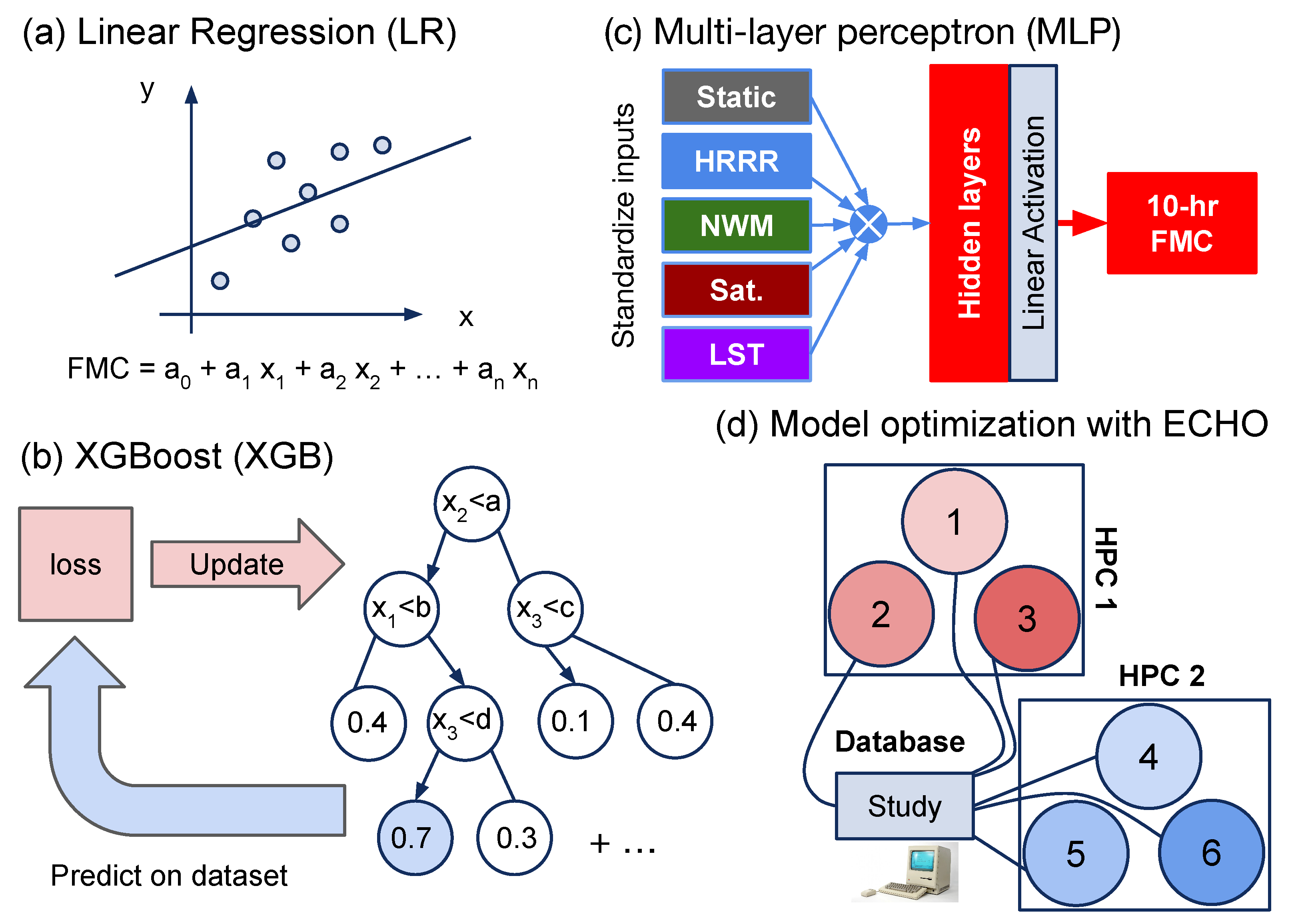As described in Section 2, the data sets that are used to train machine learning models are tabular. Only linear regression, gradient boosting approaches, and standard feed-forward fully connected neural networks are considered herein as extensive experimentation has revealed that more complex machine learning approaches do not yield superior performance [31]. Expanding on McCandless’ application, several explainability methods are herein applied to the ML models as a means of identifying the most important predictors. We also probe the most important predictors by group (e.g., VIIRS, weather inputs, etc.). These last two investigations are important for identifying whether the ML predictions make physical sense, as well as for designing a minimal model for use in operation.

One potential downside in the study by McCandless et al. is that the performances of the trained models used are likely over-optimistic due the random splitting of the data used to perform cross-validation [25]. They first split the data using 25 randomly chosen days held out as the test set. The remaining days were split randomly on site locations into training and validation sets (80/20). Random splitting essentially ignores specific space and time correlations that exist in fuel moisture content training data sets, such as that used in this study. Therefore, models to predict FMC and trained on random splits likely represent (overly) optimistic performance due to overfitting on data present in hold-out splits that closely resemble examples in the training split. A primary future objective of this study is the application of models trained on CONUS to Alaska (and potentially Canada). As VIIRS has not been in operation for nearly as long as MODIS, the data sets cover a relatively short time period (three years). Hence, sites are withheld from the training data and are only present in either a test or validation split. This way of splitting aims to break the space and time correlations across the splits. Models trained on these data, therefore, should produce more realistic performance estimates.

To assess the effectiveness of using machine learning for predicting 10 h DFMC using VIIRS and other input predictors, we structure our investigation as follows: Section 2 provides a description of the data sets used for training the ML models. In Section 3, we define the specific ML models examined in this study, along with the statistical metrics utilized to evaluate their performance. We also outline the training and hyper-parameter optimization procedures. In Section 4, we present and compare the results obtained from the trained models, emphasizing the identification of the most influential input predictors. Finally, in Section 5, we discuss the results and significance of the investigation.

2. Data Sets

The data set used to train and evaluate the machine learning models spans a three-year period (2019–2021). The following sections describe the FMC observations used in the predictand data set (Section 2.1), the predictor data sets (Section 2.2), a correlation analysis of the predictand/predictor variables (Section 2.3), and how the training data set was split to independently train and validate the models (Section 2.4).

2.1. Predictand Data Set

In order to create the 10 h FMC data set, raw FMC observations were downloaded from the Meteorological Assimilation Data Ingest System (MADIS) archive (ftp://madis-data.ncep.noaa.gov//archive/, accessed on 6 December 2022) from 1 July 2001 through 31 December 2021. This archive contains hourly compressed NetCDF files and was 2.5 T in total size. After the full archive was downloaded, fuel moisture data and site information were extracted from the hourly files and combined into yearly NetCDF files. Only sites over CONUS were kept. During this phase, sites were removed that had either missing site identifiers or inconsistent site location information. Many sites were reported with different location information throughout the year, so the site with the most recent location information was kept (i.e., site S with location X reported on 1 January 2010 would be removed if site S was reported with a different location any time after 1 January 2010). A data log containing sites that changed locations was maintained throughout the entire process. After the yearly files were created, the data from all years were combined into one NetCDF file containing sites over the CONUS region. Only sites that reported non-missing data between 2019 and 2021 were included in this file. In the end, there were 1823 RAWS sites. A QC flag was added to these files to indicate whether or not the data had passed a simple range check (0–400%).

In order to quantify the skill of ML models, we use climatographies as a reference forecast. If the ML model has lower skill than the climatography, the climatography forecast should be used, and vice versa. The skill scores are defined and discussed in further detail in Section 3.2. Two separate climatographies were created from the FMC data using only data prior to 2019, one using only the day-of-year (DOY) and another using day of the year along with the hour of the day (DOY–HR). In order to calculate the DOY climatography, each site’s data were combined over a 31-day window (15 days prior to the current day and 15 days after the current day) for all years making up the data set. For DOY 1, the climatography would consist of DOYs 351–16 (with 365 being 31 December). For leap years, data on February 29th were combined with data on the 28th. After the data were combined for each site and day of year, the average, standard deviation, and count of the total data set were recorded. A minimum of six years of data was required for each day of the year. Otherwise, the average and standard deviation were set to missing. The DOY–HR climatography was calculated similarly to the DOY climatography, except that we only used data acquired at the same hour of our target one. For example, the climatography for site S on DOY 145 at 1200Z would combine all site S data at 1200Z from 2001 to 2018 for DOY 130–160.

2.2. Predictor Data Set

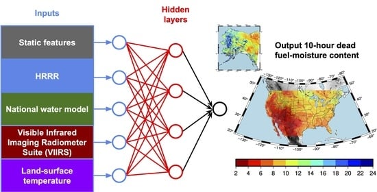
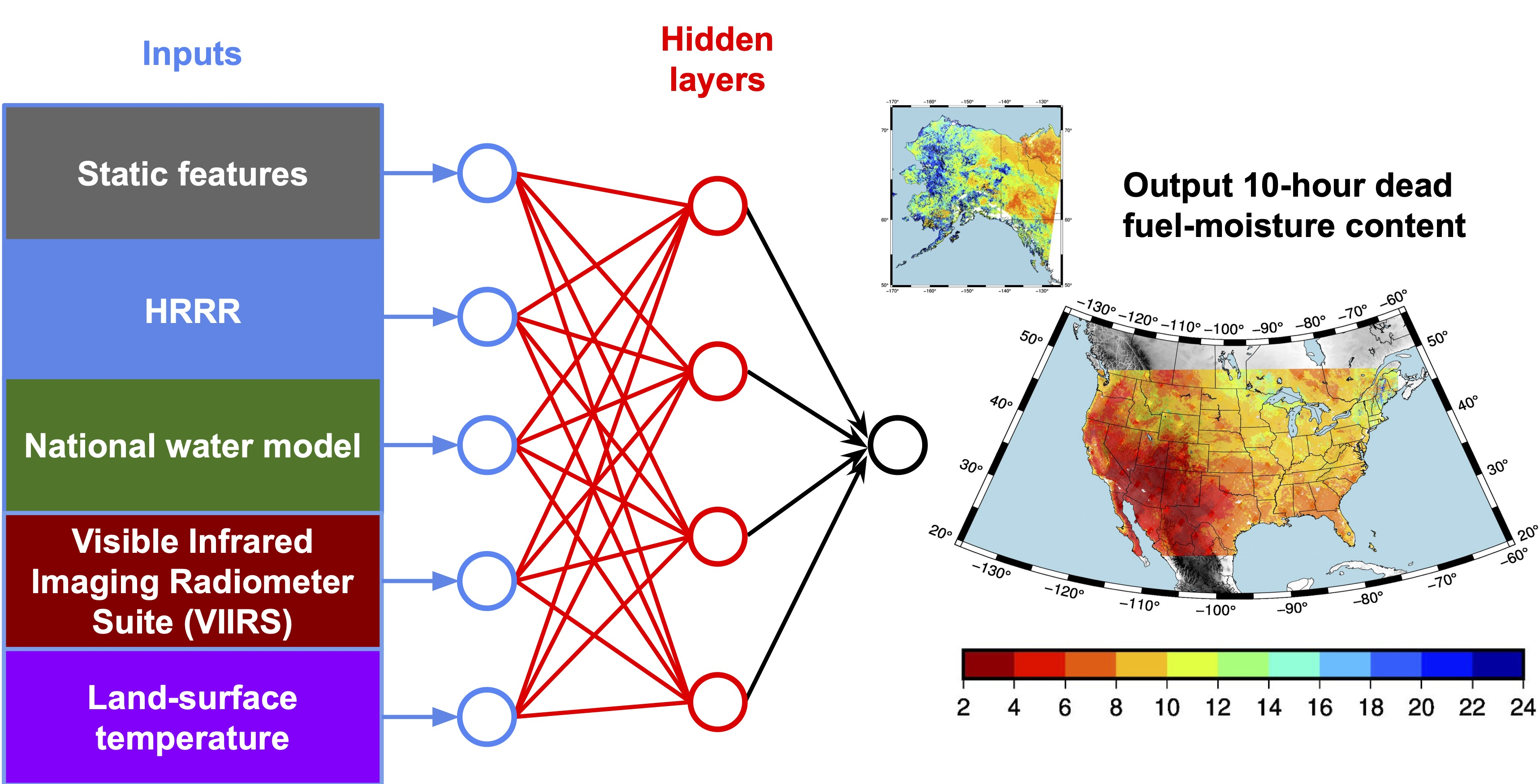
The predictor data sets consist of variables from four different sources: static variables characterizing the surface characteristics, including monthly climatographies from the Weather Research and Forecasting (WRF) Preprocessing System (WPS); analysis variables characterizing the near surface atmospheric conditions and the soil state from the High-Resolution Rapid Refresh (HRRR) model; hydrologic variables from the analysis of the National Water Model (NWM); and surface reflectance (sfc rfl) retrievals (VNP09-NRT) and land surface temperature (LST) retrievals (VNP21-NRT) from the VIIRS instrument on board Suomi-NPP. The complete list of variables is shown in

Table 1. Variables from each predictor data set. The space and time resolutions of each data set are static (1 km, 3 month climatographies), HRRR (3 km, hourly), NWM (1 km, hourly), and VIIRS (375 m or 750 m, daily overpasses over CONUS). All data sets utilized Coordinated Universal Time (UTC).

Static	HRRR	NWM	VIIRS
Canopy fraction	2 m temperature	Soil moisture	Sfc rfl M1
Soil clay fraction	2 m relative humidity	Evapotranspiration	Sfc rfl M2
Urban fraction	Soil moisture availability		Sfc rfl M3
Elevation	Skin temperature		Sfc rfl M4
Impermeability	Mean sea level pressure		Sfc rfl M5
Irrigation	Canopy water		Sfc rfl M7
Land use	Snow cover		Sfc rfl M8
Soil sand fraction	Snow depth		Sfc rfl M10
Lowest soil category	2 m dew point temperature		Sfc rfl M11
Top soil category	2 m specific humidity		Sfc rfl I1
Snow albedo	2 m potential temperature		Sfc rfl I2
Albedo clim	Cloud cover		Sfc rfl I3
Green fraction clim	Water equivalent snow depth		LST
Leaf area index clim	Global horizontal irradiance
	Sensible heat
	Latent heat
	Ground heat
	Precipitable water
	Precipitation
	Precipitation rate

.

The HRRR is an operational hourly updating numerical weather prediction model covering the CONUS with 3 km grid spacing [32]. The HRRR uses the Rapid Update Cycle (RUC) land surface model to represent the flow of moisture and energy between the atmosphere and land surface, with nine soil levels [33]. Importantly, the training and evaluation period of this study (2019–2021) spans two operational versions of the HRRR, HRRRv3 and HRRRv4. Changing versions of the model may affect the outputs, and this can introduce inhomogeneities in the time series of the variables. This can affect the training of the ML models. More details on the HRRR configuration and performance differences by version are provided by [32,34].

The NWM is an operational hydrologic model covering the CONUS at 1 km grid spacing. NWM receives its precipitation input from a variety of sources, including quantitative precipitation estimates and model forecasts, the latter of which include HRRR for the short-range predictions (out to 18 h lead time).

The predictor data sets have different spatio-temporal resolution, so some data manipulation was necessary to pair them with the predictand data set (see Section 2.1) to create the training data set. The temporal pairing of HRRR and NWM variables is straightforward since they are both available every hour, which is the resolution of the predictand data set. Some manipulation was required to pair the monthly climatographies and VIIRS data sets. The climatographies were linearly interpolated to each day of the year, whereas VIIRS retrievals were assigned to the nearest hour. The VIIRS reflectance retrievals are available for download every six minutes, and each one of these granules were assigned to the nearest hour.

All the data sets were spatially interpolated into a grid over CONUS at 375 m grid spacing. This is the grid spacing of the finest-resolution VIIRS channels (I bands). The NWM model grid spacing is 1 km. It was interpolated to the 375 m grid following a nearest neighbor interpolation. There are other methods for performing interpolation using data from more than one point; however, we selected the nearest neighbor interpolation as it is always associated with a valid retrieval for a given point. The nearest neighbor interpolation is the same approach used to interpolate the HRRR variables at 3 km grid spacing into the target grid of 375 m. In the case of VIIRS reflectances retrievals, only those retrievals without clouds or snow were interpolated into the 375 m grid. Again, the nearest neighbor interpolation was used. This is the same interpolation procedure used for the land surface temperature retrievals available at 750 m grid spacing. Only the retrievals labelled as high or medium quality were used. Finally, the monthly climatographies available at 1 km grid spacing were interpolated to the 375 m grid following the nearest neighbor approach as well.

Hence, the majority of the predictors are available at a coarser grid spacing than the target grid at 375 m. To illustrate sensitivities to the target resolution, we also independently interpolated the predictors to a 2250 m grid spacing resolution using averages of the available data within the 2250 m grid cells.

In total, 44 million data points are associated with the predictors listed in Table 1. The four predictor groups do not have equivalent temporal spacing. For example, the VIIRS are only collected twice a day, meaning that, for any one predictand (fuel moisture) value, not all predictors across the four groups will have values associated with them. We do not consider any ‘imputation’ or other strategies for filling in missing values, so the choice of which predictors are selected as model inputs will determine the total amount of data where all predictor fields have finite values and will influence a model’s prediction performance.

2.3. Predictor/Predictand Correlations

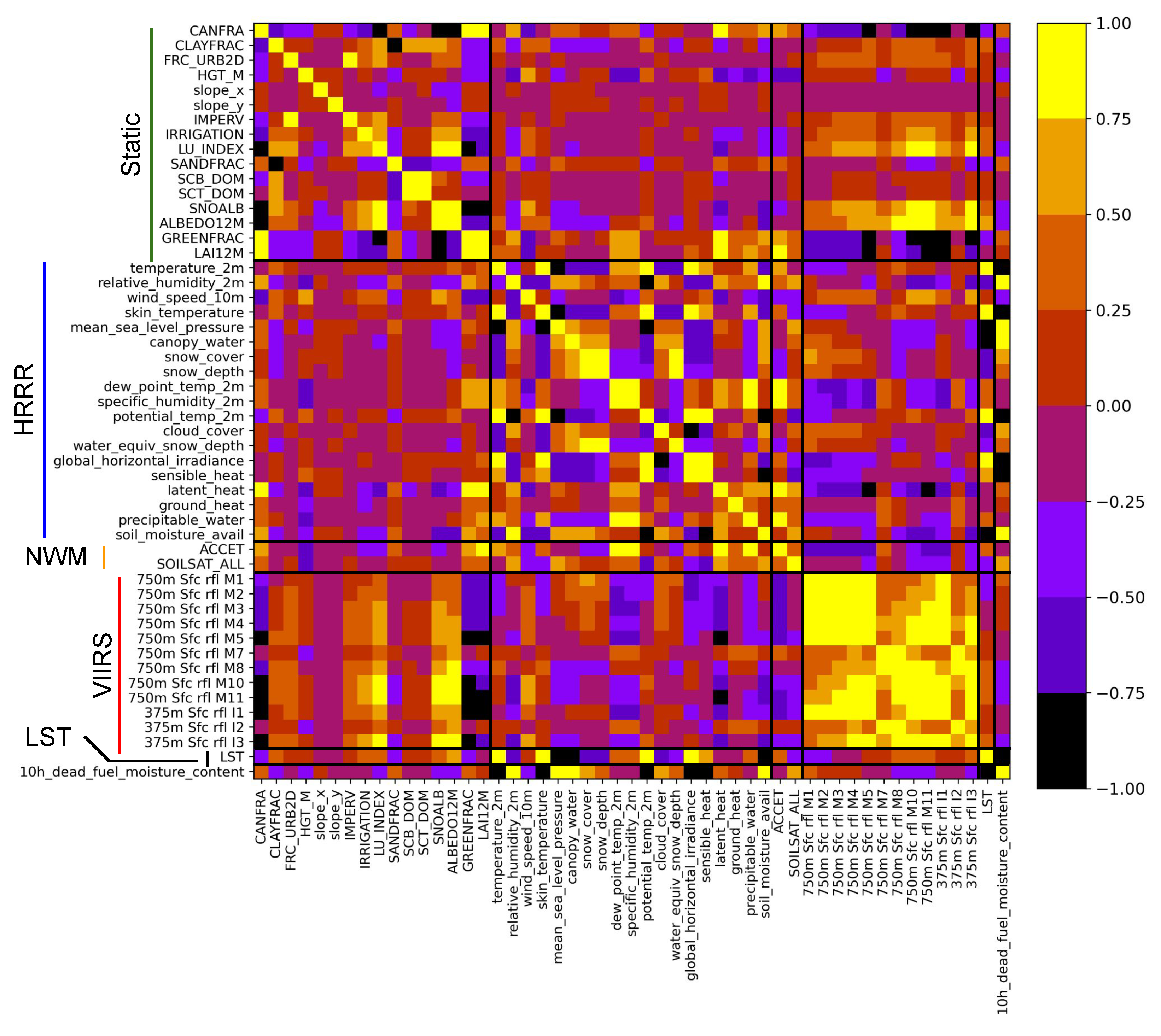
Selecting all predictors listed in Table 1, as well as the 10 h DFMC (51 in total), there are 940,000 data points where all 51 fields have finite values. Figure 1 shows how the predictors from all the groups correlate with each other and with the fuel moisture values. The figure shows that there are several HRRR predictors that are highly correlated with the fuel moisture (both positive and negative), in particular the temperature- and water-associated variables. The HRRR temperature predictors also positively correlate strongly with the LST predictor, which also has high (negative) correlation with the DFMC. The LST predictor is also modestly correlated with the M10 and M11 VIIRS bands.

Next, correlations are high among the VIIRS bands, but no one band strongly correlates with DFMC, with the exception of M10 and M11, for which the correlation is modest. The static variables, including green fraction and albedo monthly climatographies, are also observed to correlate strongly with the M8, M10, and M11 VIIRS band. However, only these and a few of the other static predictors show appreciable correlation with DFMC, and none of the NWM variables correlates strongly with DFMC.

2.4. Data Splitting and Standardization

Once a selection of input groups is selected, the resulting data set is split into training (80%), validation (10%), and testing (10%) data splits in order to train and test an ML model. Then, this is repeated 10 times via cross-validation by resampling the training and validation sets while holding the test set constant. As noted in the introduction, we consider two approaches to splitting: (1) by random selection, and (2) by randomly holding out sites (defined by latitude/longitude, of which there are about 1600 prior to 1 January 2019). The former selection does not consider that subsets of the data are highly correlated in either time, space, or both; therefore, data points that are similar may end up in both training and validation/testing splits. In the latter approach, holding out a random subset of sites from a split aims to separate out those correlated data points correctly (e.g., they all should go to the same split). In both cases, a stratified approach was also used so that all three splits effectively had a representative sample of the FMC values.

The relative ranges of all the predictors listed in Table 1 need to be transformed into a new coordinate system so that the features having the largest spread do not dominate the weight space of an ML model. During model optimization (discussed below), we found that performance was usually better when the values for each quantity listed in Table 1 and the fuel moisture value were standardized independently into z-scores according to the formula $X_j=(X_j-u)/s$, wherein u and s are the mean and standard deviation of $X_j$, so that the mean is zero and the standard deviation is one (computed on the training set and then applied to the validation and test sets). The predicted FMC value is then inverse-transformed back into the original range observed in the training data set.

3. Methods

3.1. Machine Learning Models

Figure 2a illustrates three ML models considered: (a) linear regression (LR), (b) a scalable, distributed-gradient-boosted decision tree (eXtreme Gradient Boosting, e.g., the XGBoost “model”) [35], and (c) a vanilla feed-forward multi-layer perceptron (MLP) neural network similar to those used in [36]. The LR approach was chosen as the baseline ML model because it assumes a linear dependence of the FMC on each predictor, for n total predictors, and will be the simplest model considered.

The XGB and MLP models are both non-linear and of increasing model and training complexity, both relative to LR, and often MLP relative to XGB. XGBoost is a highly optimized and regularized software implementation of the Gradient Boosting Machine introduced by Friedman [35,37]. Gradient boosting is an iterative algorithm that trains on the residuals of prior iterations in order to correct and reduce error [37], as is schematically shown in Figure 2b. The XGB model was chosen because it usually outperforms deep learning methods for tabular data sets [38] and thus is commonly recommended [31,39]. XGB also typically requires much less tuning compared to MLPs and is usually much faster to use. These are important considerations because the model is to be deployed operationally in the near future. However, neural network ensembles are often as performant as XGB, and there are more methods available to probe model explainability and uncertainties associated with model predictions, so we investigate them as well. The MLP is one of the simplest deep learning approaches, and it was chosen over more complex models, such as recurrent architectures, which are also commonly used to train on data sets with time dependence.

With the linear regression model, the values of coefficients $a_i$ in the figure corresponding with the input features $x_i$ can be computed from $n+1$ equations using least squares. The number of data points is much larger than n and thus we have a statistically robust determination of the coefficients $a_i$. XGBoost uses a weighted sum from an ensemble of decision trees to make FMC predictions (a single tree is shown in Figure 2b). Each iteration in the algorithm uses the computed root-mean-square error (RMSE) from the previous round to make the current fit. We initially also considered random forests but found them always to be inferior to XGBoost, so we only focused on the XGBoost model.

The MLP comprises a stack of N fully connected feed-forward layers and activation functions. The first input layer transforms the chosen input groups into a representation of size L and is followed by a LeakyReLU activation. The last layer transforms the latent representation of the input described by preceding layers into size one and uses a linear activation. The neural network becomes deep if there are subsequent layers sitting between the first and last layers of size L and separated from each other by LeakyReLU activation functions. After all LeakyReLU activation functions, we used a 1D batch normalization and a dropout layer, respectively.

For the MLP, the weights of the model are updated by computing a training loss on a batch of inputs and then using gradient descent with back propagation [40] along with a pre-specified learning rate to reduce the training error. Model training involves repeating this process and occasionally computing the RMSE on the validation split, then stopping training once the validation RMSE is no longer improving. We reduced the learning rate by a factor of ten when the validation loss reached a plateau.

The XGB and MLP models were both subject to extensive hyper-parameter optimization to find the best-performing models according to the RMSE computed on the validation split. We used the Earth Computing hyper-parameter optimization package to perform scaled optimization for both models, performing 1000 hyper-parameter selection trials for XGB and MLP models for random and site splits (at 375 m and 2250 m), as illustrated in Figure 2d. The first 100 trials used random parameter sampling, and then, from 100 onward, a Bayesian approach using a Gaussian mixture model strategy was employed to perform an informed search (see [41] for more details). For XGB, the varied hyper-parameters were the learning rate, the minimum drop in loss needed to make a further partition on a leaf node of the tree (denoted $\gamma$), the maximum tree depth, the number of estimators (boosting rounds), the training sub-sample rate, and the sub-sample ratio of columns when constructing each tree. For the MLPs, the varied parameters were the number of layers N, the size of each layer L, the learning rate, training batch size, the L2 penalty, and the selection of the training loss. The training loss choices were the mean absolute error, the RMSE, the Huber loss, or log-hyperbolic cosine (log-cosh) loss.

3.2. Statistical Metrics

As noted, the RMSE was used as the validation and testing metric for all three models. In addition to the RMSE, the coefficient of determination is also used as a performance metric. They are defined as

$$\begin{array}{cc}\hfill RMSE& ={\left(\frac{1}{N}{\sum }_{i=1}^N{(y_i-f\left(x_i\right))}^2\right)}^{1/2}\end{array}$$

(1)

$$\begin{array}{cc}\hfill R^2& =1-\frac{{\sum }_{i=1}^N{(y_i-f\left(x_i\right))}^2}{{\sum }_{i=1}^N{(y_i-\overline{y})}^2},\end{array}$$

(2)

wherein $x_i$ represents the ith vector input of predictors, $f\left(x_i\right)$ is the predicted ith fuel moisture value, $y_i$ is the ith true fuel moisture value, $\overline{y}$ is the average fuel moisture for the data set, and N is the data set size. To determine how well the model performance compares relative to climatographies for the DFMC, two skill scores are defined as

$$\begin{array}{cc}\hfill Skill\left(RMSE\right)& =1-\frac{RMSE\left(ML\right)}{RMSE\left(Clim\right)}\end{array}$$

(3)

$$\begin{array}{cc}\hfill Skill\left(R^2\right)& =\frac{R^2\left(ML\right)-R^2\left(Clim\right)}{1-R^2\left(Clim\right)}.\end{array}$$

(4)

A skill score larger than zero means the model outperforms the climatography on this metric (1 indicates the model is perfect), while less than zero means the climatography estimate is better (zero means the model and the climatography are equivalent in terms of metric performance).

3.3. Model Interpretation

In order to probe how the XGB and MLP training parameterization describes the DFMC values, we employed several methods to help explain the predicted outputs of the XGB and MLP models in terms of the input predictors. The permutation method measures the importance of each feature by computing the error difference before and after perturbing the feature value given some input x. Small changes in error typically indicate lower importance, and vice versa.

Secondly, the SHapley Additive exPlanations (SHAP) [42,43] method seeks to quantify how much each feature value contributed to a model prediction, relative to the average prediction, in the feature’s respective units. For example, a SHAP value for the input land surface temperature of +1 K, relative to an average value, means that the input explained that much of the predicted output value. As this example illustrates, there will be a SHAP value for each input that can be used to explain the output of either the XGB or MLP model. Formally, the SHAP value for a feature is its average marginal contribution as computed across all possible subsets of the model inputs that contain it [42].

Finally, applied only to the XGB model is the gain method for estimating importance. The gain estimates the relative feature importance according to how much the feature tree contributed to the total model FMC prediction. The larger the contribution, the more important a feature, and vice versa.

4. Results

4.1. Predictor Group Importance

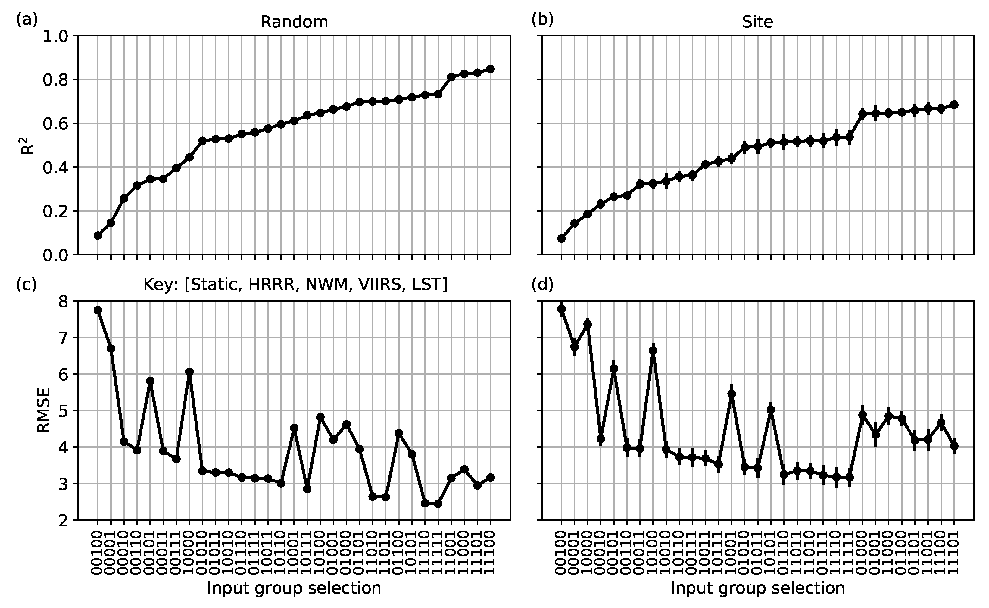
We first determined which groups were the most important to use as potential predictors by training and testing the XGB model on all combinations of the four groups listed in Table 1, plus the LST treated as its own group (hence, 31 total relevant combinations), on the 375 m data sets. The same model hyper-parameters were used. Figure 3 shows the performance metrics RMSE (bottom row) and $R^2$ (top row) for the random (left column) and site (right column) testing data splits. Both quantities were ordered by the computed $R^2$ (least to greatest). In the figure, the key denotes the usage of input features during training. A value of 1 indicates that the group of features was used, while 0 signifies that it was not used.

In the RMSE figures for both split types, the zig-zag pattern depends on the VIIRS surface reflectances set. When the reflectances are used as predictors, a clear drop in the RMSE is observed (e.g., improved performance), but there is not a similarly strong dependence in the computed $R^2$. This behavior is observed with both the MLP and LR models (not shown). The LST feature is also helpful but not necessary as the performance gains over not including it are relatively small for XGB. The importance of VIIRS reflectances as a group is due to the relatively fast equilibration times between the dead fuels (mostly sticks and brush at 10 h) and the atmosphere, which are best captured by the twice-a-day retrievals. In contrast, the NWM variables do not seem to be necessary as they hardly affect performance when used as predictors, which is reasonable because the 10 h fuel equilibrates with the atmosphere and not the soil.

In terms of lower RMSEs, the HRRR and VIIRS variables play the most important roles as predictor groups, and the (11111) models had the lowest ensemble average RMSE for both splits, with (01111) coming in a close second. Thus, the static predictors do not play a significant role in either random or site split routine. This is potentially useful for using the model outside of the CONUS (e.g., in Alaska) because the static variables are site-dependent and can be ignored as model inputs. However, this remains to be tested until Alaska data become available. Finally, the worst model in both split cases is that utilizing the NWM only.

4.2. Model Performance

Table 2. The three ML models are compared using the RMSE and R${}^2$ metrics. The rows show the metric values for the two splits (random and site) at 375 m and 2250 m resolutions. In all cases, a 10-fold cross-validation splitting routine was used to estimate the mean and standard deviation of each quantity for the testing data set.

RMSE (Split)	Linear Regression	XGB	MLP
Random 375 m (11111)	3.44 ± 0.01	2.48 ± 0.02	2.37 ± 0.08
Random 2250 m (11111)	3.65 ± 0.01	2.64 ± 0.01	2.29 ± 0.17
Site 375 m (01111)	4.12 ± 0.01	3.56 ± 0.09	3.71 ± 0.02
Site 2250 m (01111)	3.53 ± 0.01	3.04 ± 0.04	3.21 ± 0.02
R${}^2$ (Split)
Random 375 m (11111)	0.45 ± 0.001	0.72 ± 0.01	0.74 ± 0.02
Random 2250 m (11111)	0.45 ± 0.002	0.71 ± 0.01	0.78 ± 0.03
Site 375 m (01111)	0.37 ± 0.003	0.53 ± 0.02	0.49 ± 0.01
Site 2250 m (01111)	0.51 ± 0.001	0.64 ± 0.01	0.59 ± 0.01

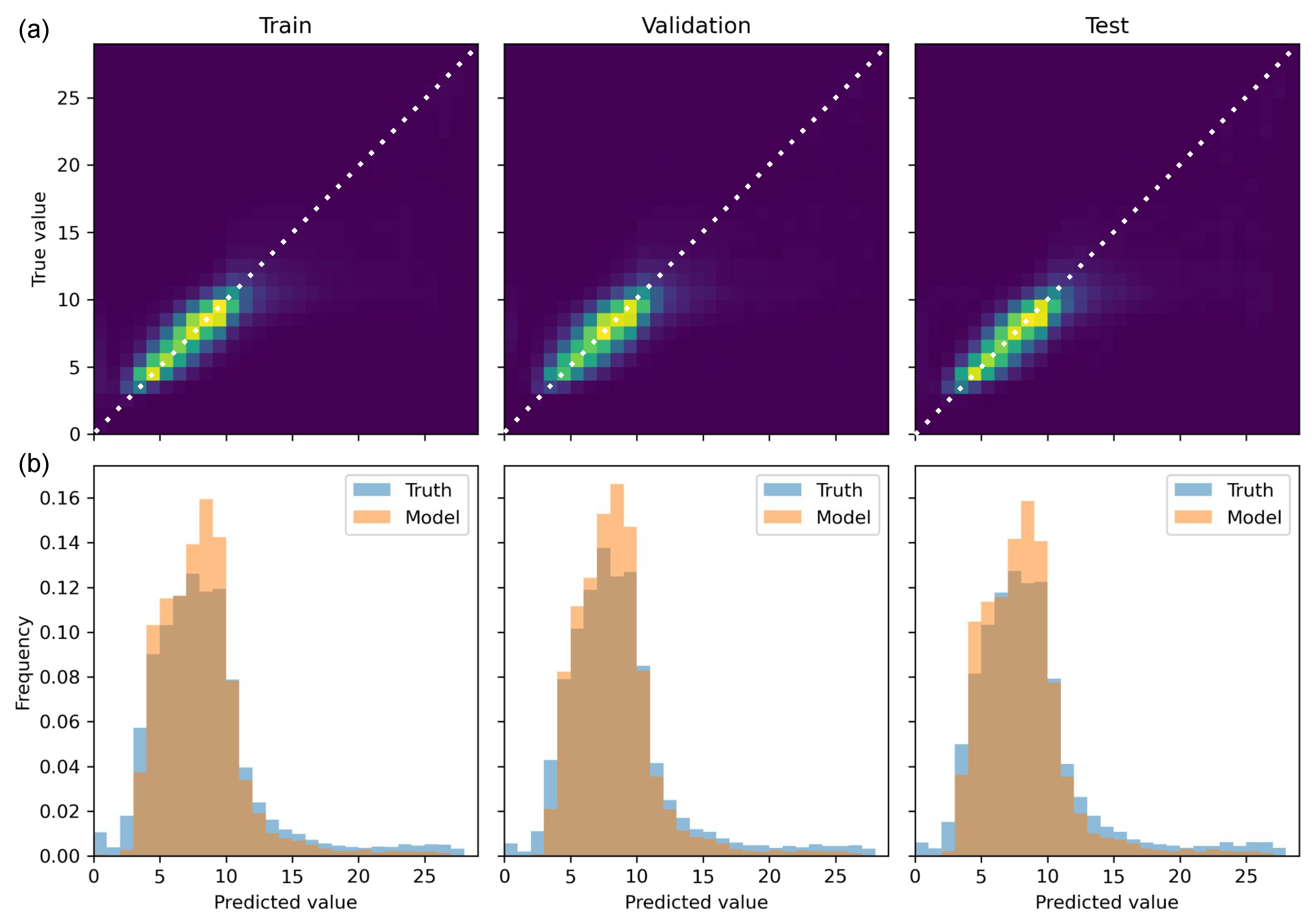
compares the computed bulk performance metrics for the LR model and hyper-parameter-optimized XGB and MLP models for the random and site test splits, respectively. Figure 4 compares the model predictions versus the 10 h DFMC targets for the training, validation, and test split for the XGB model trained on site splits at 375 m resolution. Figure 4a shows 2D histograms, while Figure 4b shows the 1D distributions for the three splits. The models trained on the random split used all predictors, while those trained on the site split left out the static predictors.

Table 2 shows that, overall, the models always perform better on the random split relative to the site split, which is expected as the random splitting most likely contains correlated subgroups of data in both training and testing splits. The performance of models trained on the site split, which represent the more realistic performance we might expect when the model is in operation over both CONUS and Alaska, is always lower by comparison. Additionally, slightly better performance is usually observed when models are trained on the 2250 m relative to the 375 m data sets (but this is not always the case for XGB).

Table 2 also shows clearly that both XGB and the MLP models outperform the LR on all metrics and on both data splits at 375 m and 2250 m resolutions. The MLP is observed to outperform the XGB on the random split, while XGB outperforms or is comparable in performance to the MLP on the site split, which did not include the static (site-dependent) variables as predictors. This is important because, operationally, XGB is much faster to use compared to the relatively large MLP model, which contains six hidden layers, each of size 6427 neurons.

The 2D histograms in Figure 4a illustrate the comparable performance of the XGB model across the three splits. The metrics reported in the table exhibit similar values for the training and validation splits, although they are not shown. Specifically, the 2D histograms reveal a clear linear relationship between the true 10 h DFMC value and the predicted value for all three training splits. In Figure 4b, similar patterns emerge among the true bulk histograms, with a prominent peak around 8 and a secondary, less pronounced peak around 25. Overall, the predicted distributions closely resemble the true distribution for all three splits. However, the model tends to predict more DFMC values around the main peak while struggling to accurately characterize the second minor peak. Additionally, the model encounters difficulties in predicting very small FMC values. These findings suggest that the model did not exhibit significant overfitting on either the validation or test splits.

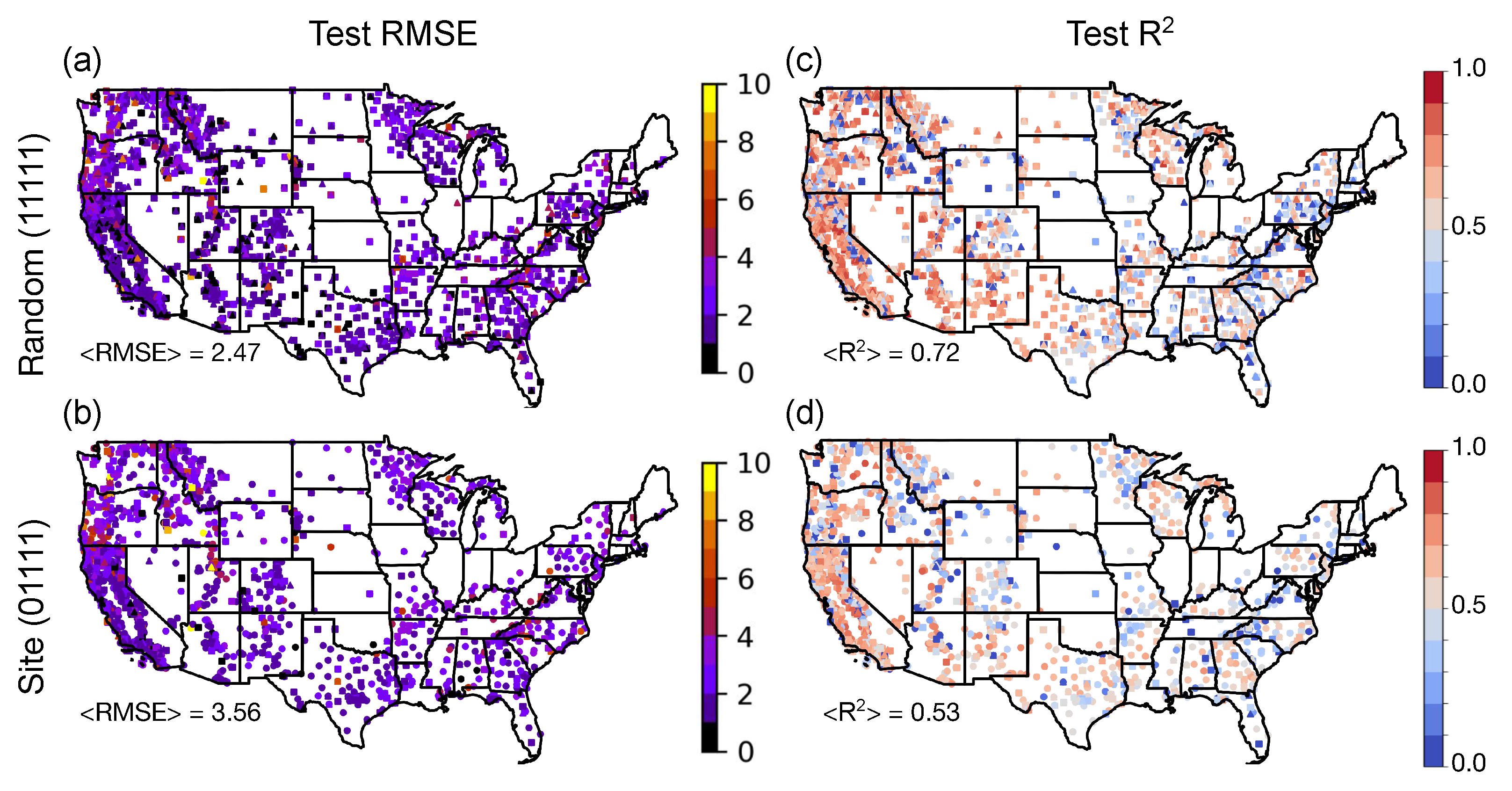
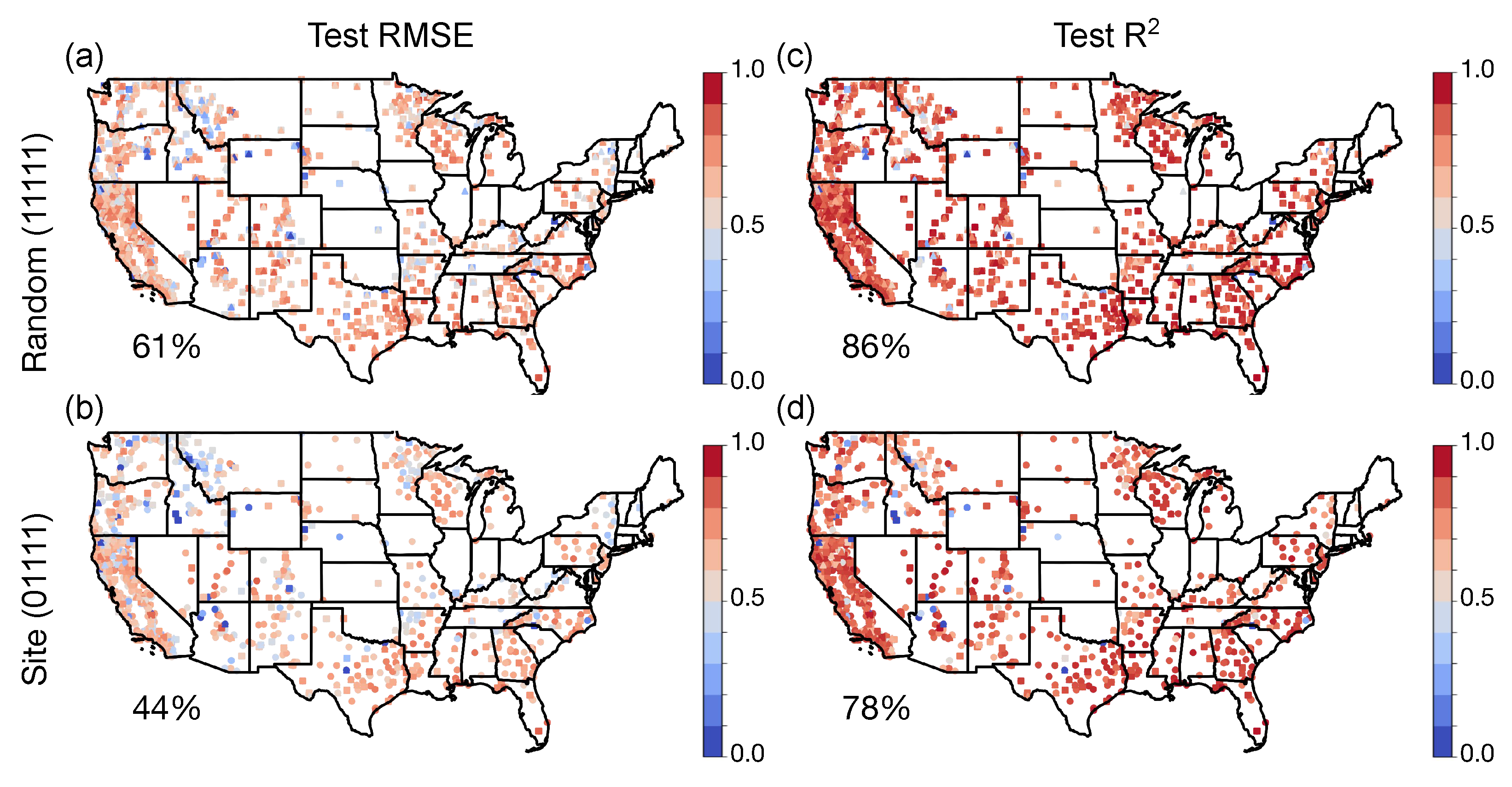
Figure 5 shows the performance metrics computed at the site level over CONUS for the XGB model trained on the 375 m site data split. Clearly, the model produces the best results in drier areas (for example, the desert in southwest and southern California, which has the lowest RMSE and highest $R^2$ scores), where the FMC does not change as much. On the other hand, the performance varies more in the Pacific Northwest, where more variability in fuel moisture is occurring, which is logically harder for the model to capture as well. The model trained on the random split shows better performance, as expected, although both models show similar trends (such as better performance in drier areas).

4.3. Model Skill

Figure 6 and Figure 7 show the spatial distributions of the model skill scores computed using Equations (3) and (4) at the site level across time using hourly and daily climatography estimates, respectively. Both the figures show that the models outperform climatography estimates for most of the sites on the CONUS map, with fairly consistent skill observed across different regions according to both RMSE and $R^2$. 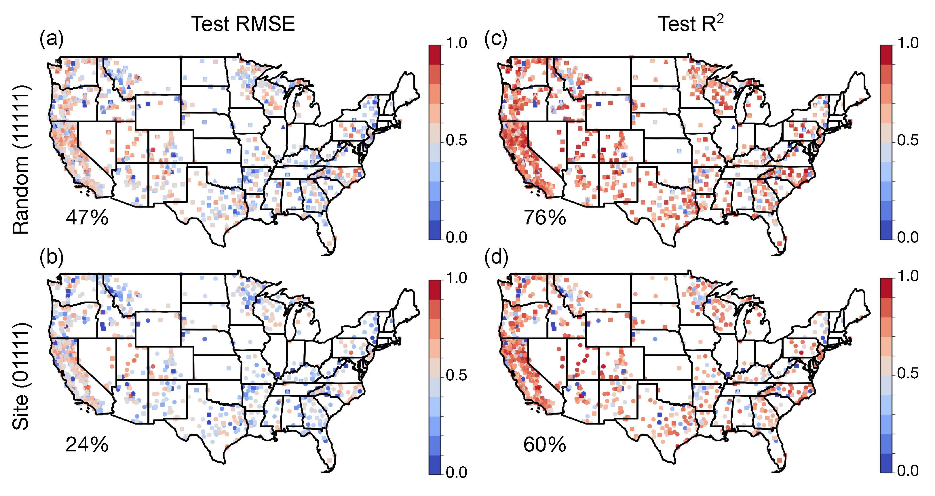The outlier sites, where the climatography estimate has the higher skill, tend to be in the mountainous west. Overall, the random and site RMSE performances improved over the daily climatography estimates by 61% and 44%, respectively. The hourly climatography is a better model than the daily climatography, and the skill scores are, as expected, smaller, with improvements of +47% and +24% for the random and site splits, respectively. Similar increases are observed with the $R^2$ skill score metric. The figures also show that the training, validation, and testing splits yielded similar results, corroborating the results from Figure 4 that the model is not too overfitted to the training data split in each case.

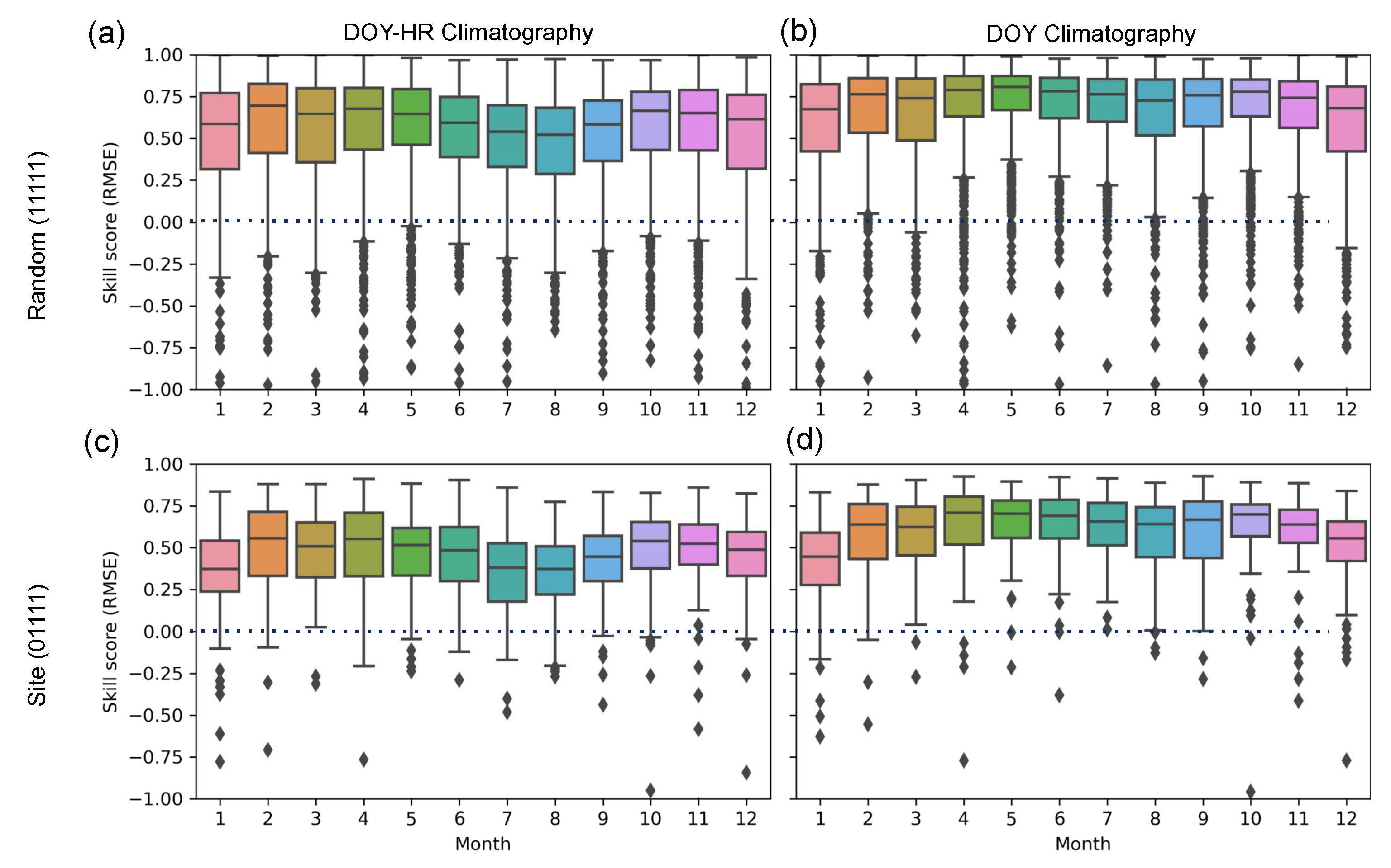
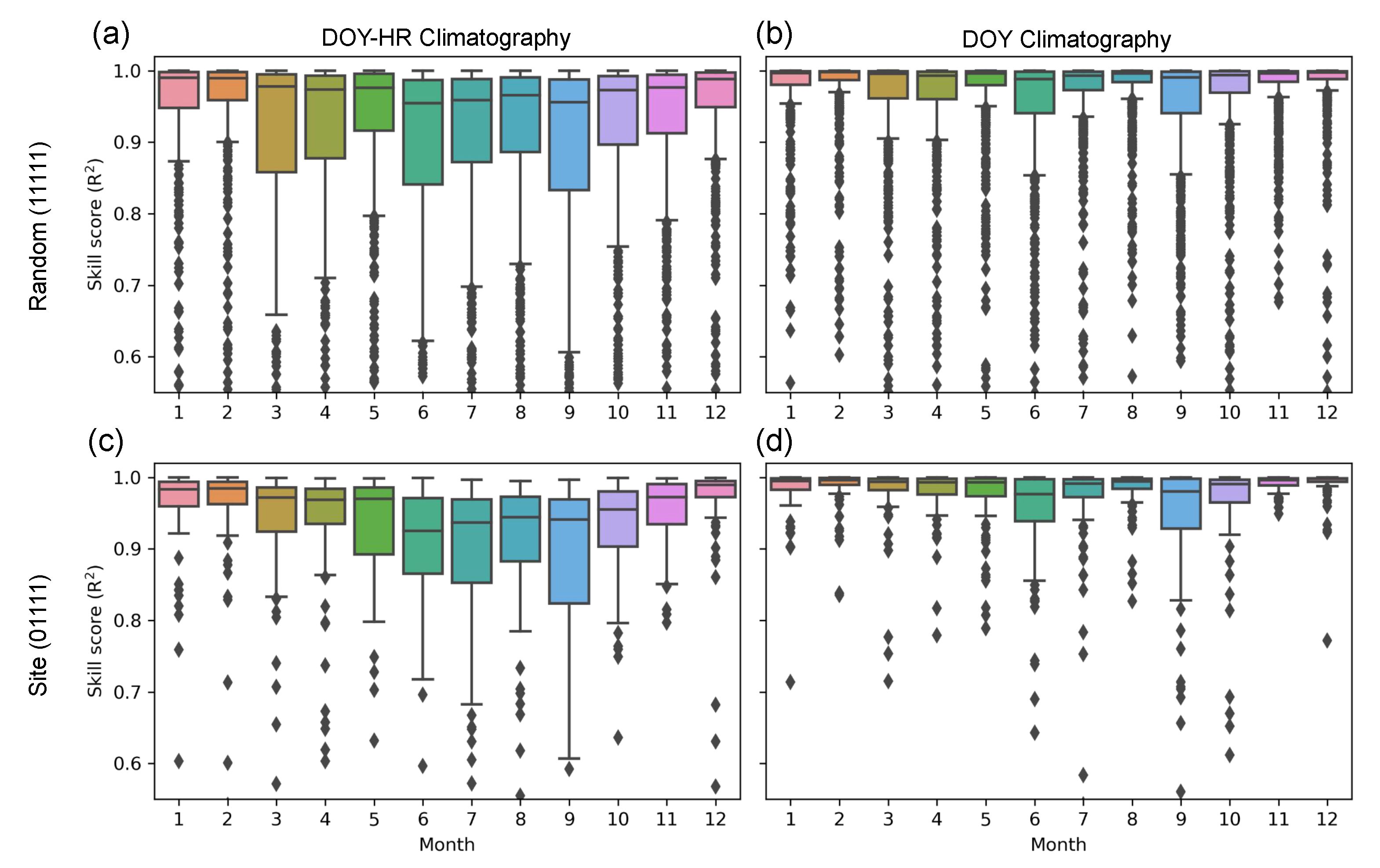
In order to understand the time dependence of the model performance, Figure 8 and Figure 9 plot the RMSE and $R^2$ skill scores for the random and site test splits by month, respectively, starting with January (1) and ending with December (12). The data points were computed by averaging over hour-of-the-day, day-of-the-year (DOY–HR) and day-of-the-year (DOY) and then grouped by month to create the box–whisker diagrams in the figures.

Figure 8 shows, for both splits and both climatography estimates, that the models are more skillful throughout the year, with more than 75% of points having skill larger than 0 at all times. However, there is still a small fraction of model predictions that are worse compared to the climatography estimates, and all outliers are less skillful than the climatography estimates of DOY–HR. By contrast, the results are improved for DOY compared to DOY–HR.

There is also a clear seasonal performance dependence when compared to DOY–HR climatography. In particular, the model RMSE performance peaks in the spring and fall and bottoms out in the summer and winter (Figure 8a,c). Model R${}^2$ performance against DOY also shows performance hitting a minimum in the summer while remaining roughly flat during the other three seasons (Figure 9a,c). The lower skill score is due to the expected larger diurnal variability in the summer. Additionally, the lower model skill on the hourly climotagraphy indicates, as expected, that hourly climatography is more skillful than daily.

Since climatography is a model local to each site, it has the inherent advantage of only introducing errors at one specific location. Our XGB and MLP models are trained using data from all sites, so errors must be minimized across all locations simultaneously. We are also not training the ML models with site-identifying information. For these reasons, we would expect the climatography of some sites to have lower error than the XGB or MLP model that was trained without site-specific data. However, we think it is worth conducting the comparison because it is sufficient to show that our model is skillful.

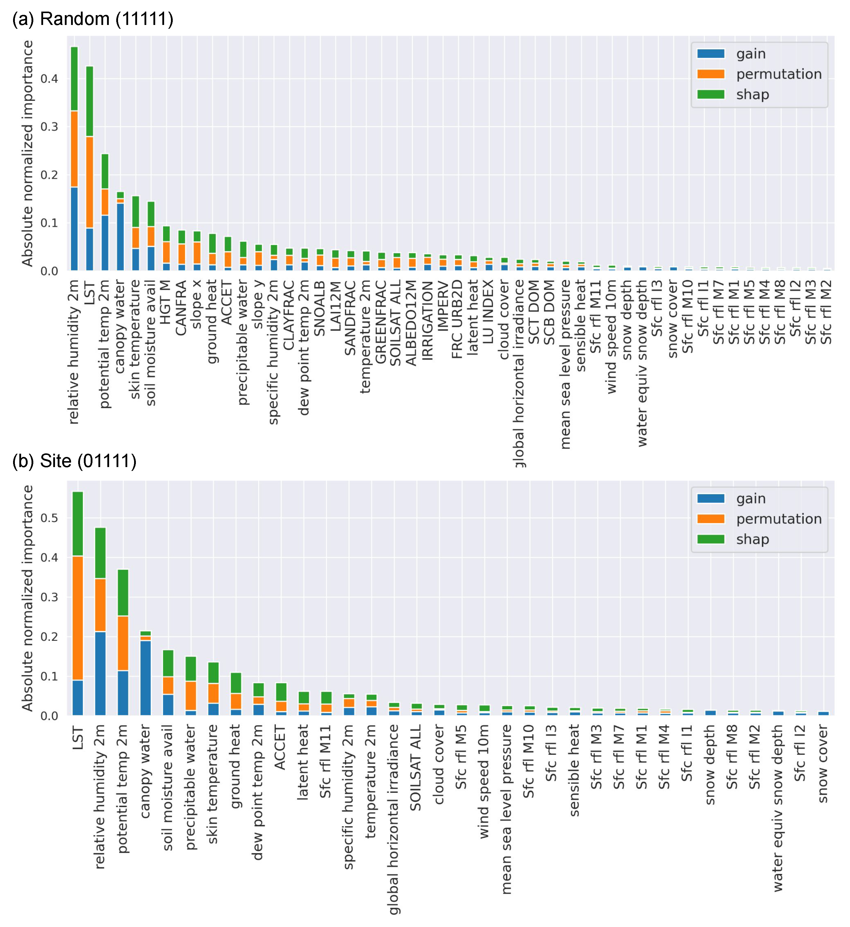
4.4. Predictor Importance

Finally, we quantify the relative predictor importance using the permutation, SHAP, and gain methods. These methods can guide feature selection, feature engineering, and model refinement processes, improving the model’s performance. Note that Figure 3 showed the dependence of the predictors as a group; the individual predictor importance allows to identify which predictors within a group are the most important. Figure 10a,b show the three computed quantities for each predictor used in random and site test splits, respectively. The figure shows the three importance metrics sorted from greatest to least importance after being summed.

Both models predict LST medium and relative humidity at 2 m as the top two predictors (in different order). Additionally, the top six of seven predictors are the same for the two models, which are LST, relative humidity at 2 m, potential temperature at 2 m, canopy water, soil moisture availability, and skin temperature. In other words, the FMC predictions are mostly explained using temperature and moisture predictors, which seems physically reasonable. The relative importance of the top five predictors also dominates those in the bottom half. However, the three methods do not rank the predictors identically. For example, the gain approach clearly differs from the other two on the importance of canopy water: it only shows that predictor being relatively significant. By contrast, the SHAP and permutation approaches suggest that precipitable water has higher importance.

The importance levels of the VIIRS reflectances are also absent in both figures, and they are always in the bottom half of predictor importance. This apparent lack of importance quantification by all three methods is due to the high correlation among the reflectances. When combined with the results from Figure 3, the VIIRS reflectances are understood to be important as a group, but any one individual band alone is not sufficient to contribute to the explanation of FMC, as Figure 10 shows.

5. Discussion

Overall, the above analyses highlight several important data and model choices, as well as deployment considerations involved in modeling FMC with machine learning. First, the performance of ML models is highly dependent on the data sources selected as fuel moisture predictors. Clearly, the most important predictor groups needed to produce skillful XGB (and MLP), relative to measured climatographies, are the HRRR and VIIRS retrievals. The VIIRS retrievals contribute as a group due to high band correlation, while a small number of individual predictors in the HRRR group have relatively high importance according to the explainability techniques used. In Figure 10, the LST predictor has high overall explainable importance, but it has low importance in Figure 3 when included as an input group. Thus, the predictor can be removed without causing a significant performance decline. This is primarily due to its strong correlation with the potential temperature at 2 m in the HRRR group. Recall that, when both HRRR and VIIRS retrievals are not used as model inputs (e.g., the surface temperature predictors are removed), the RMSE performance drops significantly (Figure 3), especially for the site split, corroborating the high importance of the surface temperature predictors (Figure 10). We also observed essentially the same group importance result for the MLP model (the results are not shown but are closely comparable to that presented for XGB). The overall importance of the two groups corroborates the dynamic relationship between the 10 h fuel and the atmosphere, and with soil moisture.

Furthermore, the XGB and MLP models are performing well relative to other FMC retrievals over CONUS. Specifically, in McCandless et al. [25], which utilized MODIS reflectance bands as input predictors, the model errors were typically 25–33% of the variability of the FMC data, while here we observed 15–20%, with the models trained on random splits having lower error relative to those trained on site splits. Other studies have reported similar errors and model performances [10,44]. With either ML model (XGB or MLP) and the current 3-year data set, we still need to know when a trained model performs better compared to climatographical baselines for it to be effectively useful; otherwise, the climatography estimates should be used. Note that the relatively low $R^2$ score for the model trained on the site split indicates that further performance improvements need to be sought after, but the climatography scores tell when the model is practically useful.

Next, the random and site approaches to splitting the data set before training ML models demonstrate the difference between an ideal scenario and expected performance when carefully preparing training and validation splits. Generally, the ML model performs worse on the site split, while the random split performs better due to the high space and time correlation between the training splits. The site split approach has an added advantage since the model validation does not depend on specific sites, unlike the random split approach. Therefore, ML models trained on decorrelated data splits may be more useful in regions outside the training data, such as Alaska, but still with similar climates and geographies. It is worth noting that both splits are not overfitted on the hold-out splits as predicted FMC distributions and testing metrics look similar across the training, validation, and testing splits. Spatially, the performance is relatively uniform over CONUS, with likely some California bias. As more data become available, these problems can be resolved. The models, including new variations, will be tested with the additional data, although, for early release, we intend to use ML models trained on the site split.

Finally, even though we primarily focused on the performance of the XGB model, the best MLPs perform similarly on the site splits and outperform XGB on the random splits. Therefore, which model should be used in deployment? For several reasons, the XGB model will be used initially. First, the optimized architectures contain millions of fitted parameters, which necessitates GPU computation during inference to obtain the best performance, as well as future training when more data are available. By comparison, even the optimized XGB found here (which is pretty large) can be orders of magnitude faster to run relative to the MLP on the GPU (depending on the overall size of the MLP). Specifically, the optimized XGB models trained on site and random splits took on the order of minutes to train and the order of seconds to evaluate the full grid over CONUS (about 1800 grid points). Depending on the size and number of hidden layers in an MLP, it may take hours (or longer) for training or inference phases.

Secondly, the MLPs are able to obtain the reported performance, in part due to the transformation of the predictors and the predicted FMC into z-scores before training the model, which requires performing the inverse transformation on the predicted FMC during inference. Even though the same transformations are applied to the XGB model (and the linear regression baseline), this is not usually required for the XGB model. Applying preprocessing transformations may limit the ability of trained models to be generalized beyond the distributions present in the training data sets, and this further represents another computational step needed during deployment. Lastly, while we did not study their performance here, the XGB model can be trained on data sets with missing values, whereas neural networks currently require masking or imputation strategies.

6. Conclusions

In summary, we have found that hyper-parameter-optimized XGB and fully connected feed-forward neural architectures are both skillful with respect to hourly and daily climatographies for the task of 10 h DFMC prediction. By exploring all combinations of input groups, the main predictor sources are found to be from HRRR and VIIRS. In particular, the most important HRRR predictors are those relating to temperature near the surface and available moisture. By contrast, the VIIRS bands seem to be important only when included as a group rather than any one band dominating either models’ explanations. This latter finding is the result of fast equilibration of 10 h dead sources and the atmosphere and soil. Even though the models provide better estimates relative to known climatological estimates, by including more diverse and comprehensive data, the models may capture additional information and relationships that contribute to more accurate FMC estimates. This and the prediction of live FMC are the main objectives for future studies.