1. Introduction
The last decade has seen an exponential increase in the application of embedded systems within the automotive industry; this modernization has allowed for deeper and more complex integration of electronics, in part fueled by higher interest in electric and hybrid vehicles. This phenomenon has led to a wave of demand for vehicles equipped with ADAS (Advanced Driver Assistance Systems) and “self-driving vehicles”, shifting automated driving into a particularly pertinent field of research. This increased interest has been accompanied by a requirement for better and more accurate machine learning models, in turn necessitating new performance indicators and metrics, higher quality and diversity of evaluation methods, and higher quality and realism of the datasets used to train these models, among others.
Nevertheless, accidents involving autonomous vehicles have been reported as a result of errors in the perception computing layers [
1,
2,
3]. One such example involved an accident between one of Uber’s vehicles and a pedestrian holding a bike while crossing a street. Reports suggest that while both the LiDAR (Light Detection and Ranging) and RADAR (Radio Detection and Ranging) systems detected the pedestrian about six seconds before the registered impact, a misclassification of the pedestrian as an “unknown object” led to the unfortunate crash [
3]. Despite development efforts held in the past years, further research is required to prevent these failures. Special attention must be paid to ways in which researchers may improve or characterize the performance of perception algorithms, especially under diversified driving situations. Notably, the literature cites an acute lack of research involving holistic LiDAR data [
4].
This may be due to the fact that LiDAR usage within vehicles is a fairly new field of application, with the required technology having improved steadily over time. Earlier versions of integrated LiDAR systems showed a lack of fidelity and resolution in the obtained point clouds, with each subsequent iteration providing denser and more precise measurements that allow for fewer mistakes within the perception layer. As noted in [
4], an overwhelming amount of research effort has been placed on multi-source imagery obtained with cameras, RADAR, LiDAR, and multimodal research being scarce at best.
Fundamental requirements in obtaining robust and accurate perception algorithms lie in expanding availability and size of datasets, improving the effectiveness of testing methods and relevance of key performance metrics, and mitigating risks by better assessing the performance and evolution of these algorithms. There are a few ways to achieve this, notably by comparison of the layer’s output against a “ground truth” (labeled data) that makes up part of the dataset. Other notable approaches involve the collection of detailed and relevant data via thorough testing, analysis of correlations between metrics, detection of anomalies and outliers, identification of fringe cases, and notable exceptions, among others [
4,
5].
This paper reports preliminary results obtained through a novel multifaceted approach based entirely on LiDAR data. The proposed algorithm shows the ability to outline points of concern within a dataset by highlighting likely anomalous point clouds, the discernment and classification of which can be difficult for perception algorithms, as well as to complement other performance evaluators. By coupling this methodology with other techniques, different and more effective analysis can be obtained. As an example, by coupling a simple IOU (intersection-over-union) analysis with the proposed methodology, it is possible to know which inferred bounding boxes fail to match the ground truth as well as why such a mismatch may have occurred. In this case, should the anomaly score prove low (i.e., a false positive), it can be inferred that the misclassification occurred as a result of similarities between the object’s point cloud and the idealized point cloud for that category, such as a vaguely car-shaped piece of architecture or vegetation. Otherwise, it can be inferred that the anomaly occurred solely due to an error in the algorithm’s classification.
With this approach in mind, we may leverage its unique characteristics to aid in the training and evaluation of perception algorithms. Its ability to identify possible outliers within a particular category allows for the detection and removal of data which may prove unsuitable for a given purpose, facilitating the building and use of a dataset. Furthermore, through a similar process this method is able to calculate the probability of a given LiDAR point cloud (PC) belonging to a certain category.
1.1. Mathematical Copulas
In probability theory and statistics, a cumulative distribution function (CDF) provides the probability of a given variable
X taking a value less than or equal to
p. A copula
is a distribution function having marginal laws that are uniform in
. This is a special multivariate cumulative distribution function case; the marginal probability distributions for each of the variables that define it are uniform on this interval, allowing them to be separated from the dependency structure associated with a multivariate distribution [
6] and the following three conditions to be verified:
If
C is a copula related to a random vector
, then
C couples the distribution functions in the sense that
While at first glance copulas may appear to be niche, they can be applied in a wide variety of ways. First, it is known that by leveraging the Central Limit Theorem via the sampling of a given distribution, it can be transformed into a uniform distribution. Furthermore, any uniform distribution can be transformed into any given function via inverse sampling [
6]. Considering this, Sklar’s Theorem [
7] can be introduced, stating that any given multivariate joint distribution can be written in terms of a univariate marginal distribution, and as such can be described by a copula [
6].
Due to these properties, copulas have long been used to describe the correlation between seemingly random variables, finding applications in many fields. Most notably, they are widely used in finance to manage and optimize investment risk. Recently, copulas have found new applications in a variety of fields, including outlier detection [
6], software quality assessment [
8], automotive component failure [
9], testing of analog and mixed-signal circuits [
10], and fault detection in mechanical engineering [
11].
For the purpose of automated driving, LiDAR scanners operate by firing a sequence of laser beams with a wavelength in the infrared spectrum towards the surrounding environment. After calculation of the laser beams’ roundtrip time considering the beam intensity upon reaching the scanner, the LiDAR software is then able to map the surrounding area using a specific amount of points that depends on the LiDAR’s resolution. Sensors specifically made for advanced vehicle safety provide vertical × horizontal surround angle views of with – resolutions and 100 m to 300 m range with cm accuracy. Each of the points in a PC represents a radial distance, identified by polar coordinates, which can be translated into their Cartesian counterparts. With this information, LiDARs are able to obtain a reflectivity index from the aforementioned captured beam intensity.
1.2. LiDAR Data Analysis
The task of a LiDAR data perception algorithm is to interpret and process the information conveyed by the captured PC in order to detect and track objects. Accurately segmenting the captured PC into the various objects that compose a scene and locating them in the 3D space is not a trivial task, especially when the relative distance, shape, and size of objects are required. At times, the assessment accuracy of an algorithm may be directly correlated with the available LiDAR data resolution and the quantity of captured points, with sparser PCs leading to greater gaps in the PC density and as such being more error-prone. It is equally as important to note that captured PCs are usually noisy, sparse, and inconsistent due to extrinsic factors such as complex geometries, unforeseen occlusions, differences in reflectivity, and severe weather conditions. Performance degradation due to aging, wear, and tear on the LiDAR system are other possible reasons for poor quality of the PC. Due to these issues, it is not uncommon to find scattering within PCs and displacement of points into positions that may be seen as anomalous.
Prior to presenting the obtained preliminary results, the following section provides a summary revision of several methods used to test and evaluate different aspects of automated driving system functionality, including perception algorithms and the associated data.
Section 3 presents an in-depth explanation of the proposed methodology, including an overview of outlier detection and the detector developed in this work, as well as a presentation of the analyzed data and the method we wish to outline.
Section 4 discusses the preliminary results obtained after applying the proposed methodology, making use of the KITTI dataset [
12]. Finally,
Section 5 highlights our main conclusions and identifies additional ongoing work being carried out on the ways in which LiDAR resolution and point cloud density can impact the performance of perception algorithms.
2. Overview of LiDAR Data Testing Methods
The correctness of a LiDAR PC is usually evaluated by calculating the minimum Euclidean distance between equivalent points in both a reference and the captured PC. Four metrics are typically used: the Hausdorff Distance [
13], Modified Hausdorff Distance [
14], Chamfer Distance, and Earth Mover’s Distance [
15]. The LiDAR’s accuracy is then provided by the Root Mean Square Error of the calculated distances. However, the simple calculation of these distances does not allow for the detection of outliers or their probabilities.
The detection of outliers in LiDAR data in agricultural applications has been previously discussed in [
16]. The authors evaluated two methods. One is based on a geometric approach in which noisy point cloud data are fitted to a surface via normal and curvature estimation in a local neighborhood. The other relies on the PointCleanNet (PCN) deep learning framework. It is considered a simple data-driven method for removing outliers and reducing noise in unordered point clouds while being able to handle large densely sampled point clouds. While the first method requires the specification of input parameters that are sensitive to the distribution and density of the points in the dataset, the second proves to be more robust against changes in the point cloud density, shape, and level of noise. Nevertheless, PCN typically requires point densities greater than about 600 points per m
; moreover, as a supervised learning method, it is unlikely to succeed when the training noise characteristics differ from those of the test data.
A 2020 publication analyzed the performance of various LiDAR types available on the market [
17]. The authors sought to better understand how their respective performance differences would impact the safety of future automated driving systems. The capabilities of ten LiDARs were evaluated using various metrics that encompassed twelve manufacturers’ specifications: channels, frames-per-second (FPS), precision, maximum range, minimum range, vertical field of view (vFOV), vertical resolution (vRes), horizontal resolution (hRes), wavelength (
), sensor diameter (
d), weight, and price.
First, the authors began with a set of qualitative observations to analyze each LiDAR’s performance regarding secondary reflections, intensity-based aberrations, blooming, missing points, and traffic line visibility issues. These observations were intended to identify the main contributors to PC noise, measurement errors, artifacts, scarcity, and missing information. A statistical method was used to measure the respective overall accuracy and precision. The methodology was detailed, allowing for reproducible results by using the relative error and root mean square error across three different targets for each LiDAR. This same methodology was then extended to measure the impact of surface reflectivity on the LiDAR data by making use of the different material properties of each target [
17].
A similar analysis was used on a smaller scale to assess the impact of each individual laser on the overall PC. The end goal was to ascertain whether accuracy errors resulted from faults in the calibration procedure of individual lasers or from the sensor’s attempts to compensate for differences between its laser emitters. It was found that most LiDAR errors are due to the latter [
17]. A final point of concern addressed the density of points within a given PC, seeking to compare experimental results with the expected maximum provided by the datasheet specifications. The expected density of points can be calculated using the LiDAR’s sampling rate and frequency, field of view, and resolution specifications. By knowing how many points are obtained after a given amount of frames, verification of successfully returned laser beams allowed the authors to compare the theoretical and practical density of the beams as well as the differences in their intensity [
17].
In 2021, a review of the methods used to test environmental perception in automated driving systems was published in [
18]. In this work, the authors found that while much of the testing and evaluation present at the time conformed to ISO 26262 [
19] and ISO 21448 [
20], this became insufficient when vehicles received a greater degree of automation. They highlighted several points regarding the interdependence of criteria and the inability of existing metrics to account for points of failure which, while not formally regarded as catastrophic failures, may nonetheless result in accidents.
One such highlighted example involves a metric dubbed the “
statistical safety impact” [
18], which evaluates a system’s safety impact in individual scenes. Unfortunately, this metric depends on whether the system itself correctly recognizes and reports its uncertainty. If a failure-induced mischaracterization occurs, an uncertainty may never be detected, in which case the abnormality remains undetected. Similarly, there are times in which the perception layer may encounter uncertainties around a false positive, such as cases involving “ghost pedestrians”. This may cause the subsequent layers to behave erratically, leading to emergency maneuvers and dangerous breaking that can place other vehicles and drivers at risk. Most of all, their review highlights that despite the existence of safety criteria and metrics which fulfill them, including those independent from the system itself, there exists a pressing need to produce new and more apt indicators that do not rely on the system itself, are able to consider the impact that a misclassification might have on the entirety of the system pipeline, and are scalable to higher degrees of autonomy.
In 2022, a thorough survey was published by [
4] that delved into the many forms in which anomaly detection has been leveraged to tackle this specific context, outlining an extensive list of previous methodologies developed throughout the years. They identified five distinct categories: confidence score, reconstruction, generation, feature extraction, and prediction. For each category, the authors searched extensively for any methods that could be applied in a given context, identifying three main modalities for data capture: camera, LiDAR, and RADAR. Additionally, analyses were conducted regarding the detection of anomalies across multimodal facets and object-level data. The former encompassed data captured with two or more of the previous three modalities, while the latter involved abstract abnormalities such as behavioral patterns and other data not bound to any given modality.
Within their survey, the authors highlighted the differentiation between the quantity and the quality of effective methods, especially concerning data captured by LiDAR. Of all the modalities, LiDAR presents the least technological development when it comes to the identification of anomalous data, comprising only four total methods, three in the confidence score category and one reconstructive approach. While per-point detection is a well-explored field of anomaly detection, object-level and pattern-based approaches remain few and far between.
3. Materials and Methods
To better contextualize this description, a basic overview of the utilized tools and materials is introduced before presenting the actual procedures, starting with a brief explanation of the COPOD algorithm.
3.1. Outlier Detection
Outliers, typically regarded as anomalies, are commonly understood as instances, actions, or objects which fall outside the norm. In the field of statistics this refers to unexpected datapoints or patterns which do not conform to an expected behavior [
21]. This definition can be further explored by taking an abstract set of data describable via a given number of functions. In this case, outlier designates any point unable to be fit into at least one such function, originating instead from an unknown distribution foreign to the remaining data. Conversely, any points which can be fit into these describing functions are regarded as inliers.
Outlier detection refers to any process which may be used to accurately identify such anomalies through the separation of inliers and outliers [
6]. Depending on the quantity, type, labeling, and other such characteristics of a given dataset, the manner in which such anomalies are identified necessarily varies. With this in mind, it is possible to distinguish between three main types of algorithms which are fundamentally characterized by the availability of labels in the dataset [
21].
Supervised detection relies on fully labeled data, and often benefits from the use of classifiers to deal with unbalanced class distribution.
Semi-supervised detection is characterized by training data which consist only of normal instances without anomalies.
Unsupervised detection is performed on unlabeled data, taking only the intrinsic properties of a dataset.
Copula-Based Outlier Detection
An outlier detection algorithm based upon copulas was first introduced in Li et al. [
6]. In this publication, the authors provided a comparison between their at the time novel approach and its closest competitors. Highlighted in the showcased results are direct comparisons between these algorithms focusing on the differences in speed and performance, both of which COPOD excels at. Notably, the authors highlighted its statistical approach and complete lack of hyperparameters as two of the most distinguishing factors [
6].
These characteristics allow for ease of use, removing any need for manual tweaking or tinkering, which in turn leaves little margin for user error. Furthermore, as it is able to function either with and without learning splits, it can operate as a supervised, semi-supervised, or unsupervised algorithm. It has been integrated into the pyOD (Python Outlier Detection) [
22] suite, which allows for further accessibility.
The algorithm itself is based on the exploitation of properties intrinsic to empirical copulas, which can be derived from eCDFs (empirical Cumulative Distribution Functions). A CDF is a descriptor of the probability of a given variable
X taking a value less than or equal to
p. The continuous nature of this probability distribution, however, imposes rather expensive computational requirements which do not scale well in multivariate cases. An eCDF can be used instead, defined as a step function which approximates the true CDF via a sampling system with a frequency of 1/n, with n being the total amount of samples.
Figure 1 shows the eCDFs obtained from a CDF when considering 25, 100, 1000, and 5000 samples, respectively. As can be seen, the reduction in the number of samples implies higher deviation from the original CDF, and the confidence interval is wider. A copula is a special case of a multivariate CDF defined by the uniformity of each variable’s marginal probability in the interval of
.
The COPOD algorithm works through a three-stage process, taking a dataset of a given dimension and size and outputting a linear vector of that same size that contains the outlier score for each datapoint. These scores, represented by a positive real number, are not an indication of a given datapoint’s outlier probability; instead, they provide a relative measure of the likelihood that a given datapoint is an outlier in relation to the rest of the dataset [
6].
The first step in achieving this output begins with the algorithm fitting emperical CDFs for both the left and right tails. A skewness vector is calculated as well, which is used later on to combat any inherent biases presented by the dataset. Then, the algorithm computes the empirical copula observations for each datapoint while using the previously acquired skewness vector as needed to correct any possible bias. With these observations, the algorithm can proceed to the final step, calculating the probability of observing a point at least as extreme as each other datapoint across each of the dataset’s dimensions. In this context, extremity can be defined via the tail probability; the smaller the tail probability, the higher the likelihood that a given datapoint is an outlier [
6].
The previously computed observations allow the algorithm to know the degree of extremity of each datapoint, and consequently the relational value between them. Using this, it calculates the maximum of the negative log of the probability generated by each tail and the skewness-corrected empirical copulas, then uses it to represent the outlier score. Taking the definition of extremity into account, this is intuitive, as the minus log is inversely proportional to the tail probability [
6]. The pseudocode of the algorithm is provided in Algorithm 1.
3.2. Data
For the purposes of this first introduction to the methodology, we elected to use the KITTI (Karlsruhe Institute of Technology and Toyota Technological Institute) dataset [
12]. KITTI has been a benchmark of autonomous driving datasets ever since it was made available in 2012, providing a stereo camera and LiDAR data (four features:
x,
y,
z, and intensity) via a 360
Velodyne Laserscanner [
12]. The 2017 version of the 3D Object Detection Evaluation dataset provides 7481 training images and 7518 testing images, corresponding to a total of 80,256 labeled objects across multiple categories such as ’Car’, ’Van’, ’Truck’, ’Pedestrian’, ’Person (sitting)’, ’Cyclist’, ’Tram’, and ’Miscellaneous’ [
24].
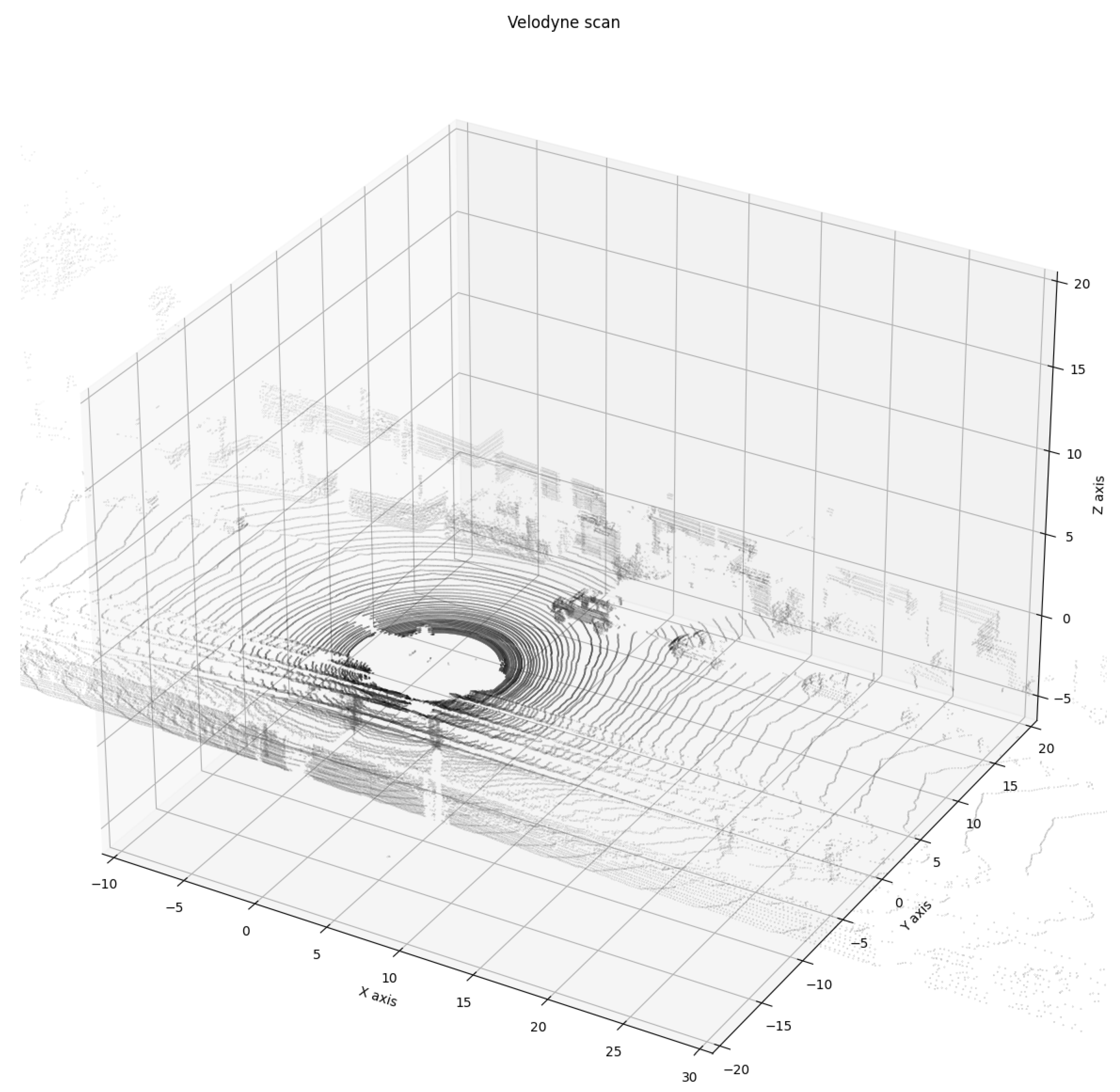
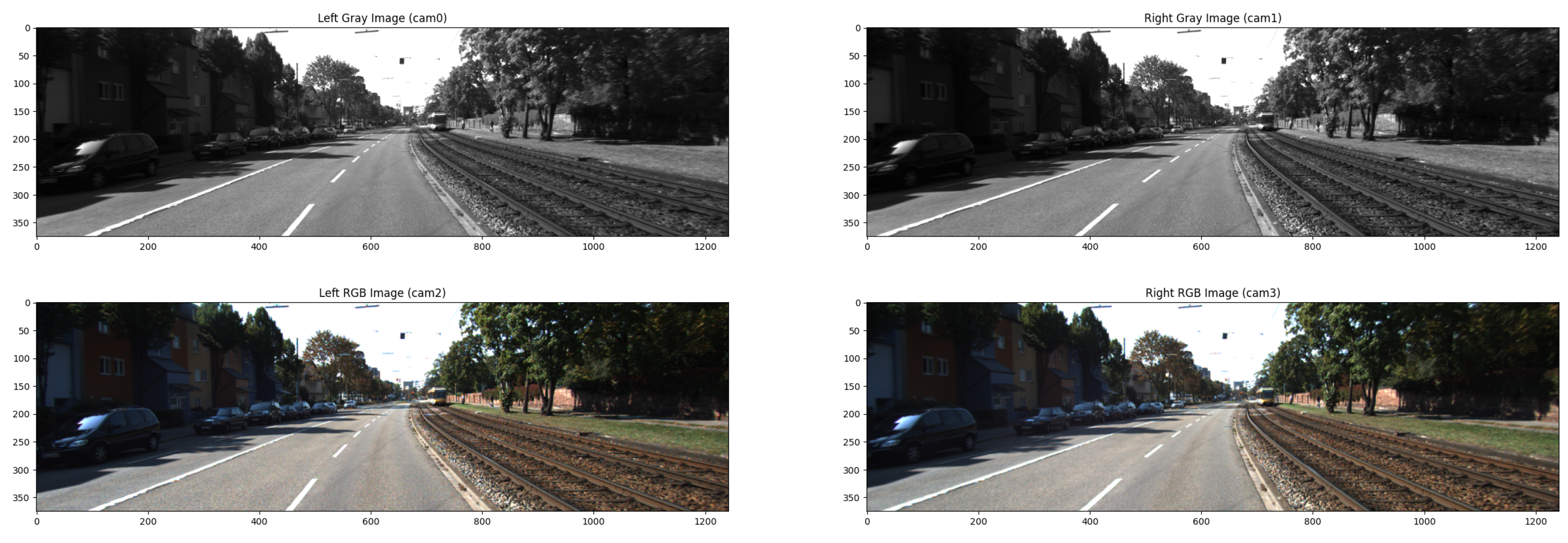
The data are separated across different .zip files, which contain left color images, right color images (stereo dataset), Velodyne point clouds, and the labeling data for the training portion of the dataset [
12]. Pictured in
Figure 2 and
Figure 3 are a single frame’s LiDAR point cloud and the associated camera views.
| Algorithm 1 COPOD Algorithm [6] |
| Input: Data |
| Output: Vector |
| 1: | for each dimension d do |
| 2: | Compute left tail ECDFs: |
| 3: | Compute right tail ECDFs: |
| 4: | Compute the skenewss coefficient: |
| 5: | end for |
| 6: | for each i in 1,...n do |
| 7: | Compute the Empirical Copula Observations: |
| 8: | |
| 9: | |
| 10: | |
| 11: | Calculate tail probabilities of as follows: |
| 12: | |
| 13: | |
| 14: | |
| 15: | Outlier Score |
| 16: | end for |
| 17: | return
|
There are a few ways in which to extract and organize the available LiDAR data. One is to extract the data pertaining to each point within a given bounding box, thereby shaping the coordinates into a position relative to the bounding box’s center. This is a necessary step when eliminating inconsistencies in an object’s point cloud that may arise due to the distance to the scanner itself, and allows each resulting collection to better describe the captured object’s shape. These data can be stored in individual NumPy arrays for later processing.
3.3. Methodology
The peculiarities of COPOD as a multivariate statistical method render it unable to parse the previously acquired data. Its input is constrained, accepting only a collection of one or more features or variables that it can relate and process. The associated matrix must be strictly uniform, and must be either one- or two dimensional.
This poses a problem, and required restructuring of the data to ensure proper processing by the algorithm itself. To this end, we looked to the x, y, and z coordinates as individual features through which to fit the algorithm. In this way, the eCDF and subsequent copula derived from the conjunction of all these points were able to accurately describe the shape of a given category. Looking at the granularity present in the KITTI dataset, cars and vans are regarded as different entities, as are trucks and other vehicles. This means that a ‘Car’ is a somewhat defined entity with a shape that, while different individually, can be characterized by telltale characteristics easily picked up by a LiDAR point cloud.
With this in mind, it is important to note that this approach disregards crucial information and granularity derived from individual contexts or from the intrinsic properties of distinct cars, which could help to better identify outliers or in preventing misclassification. In these first experiments, the intensity data were not considered; however, because a copula is a multivariate distribution function, this information could be included as long as the intensity data are restructured as well.
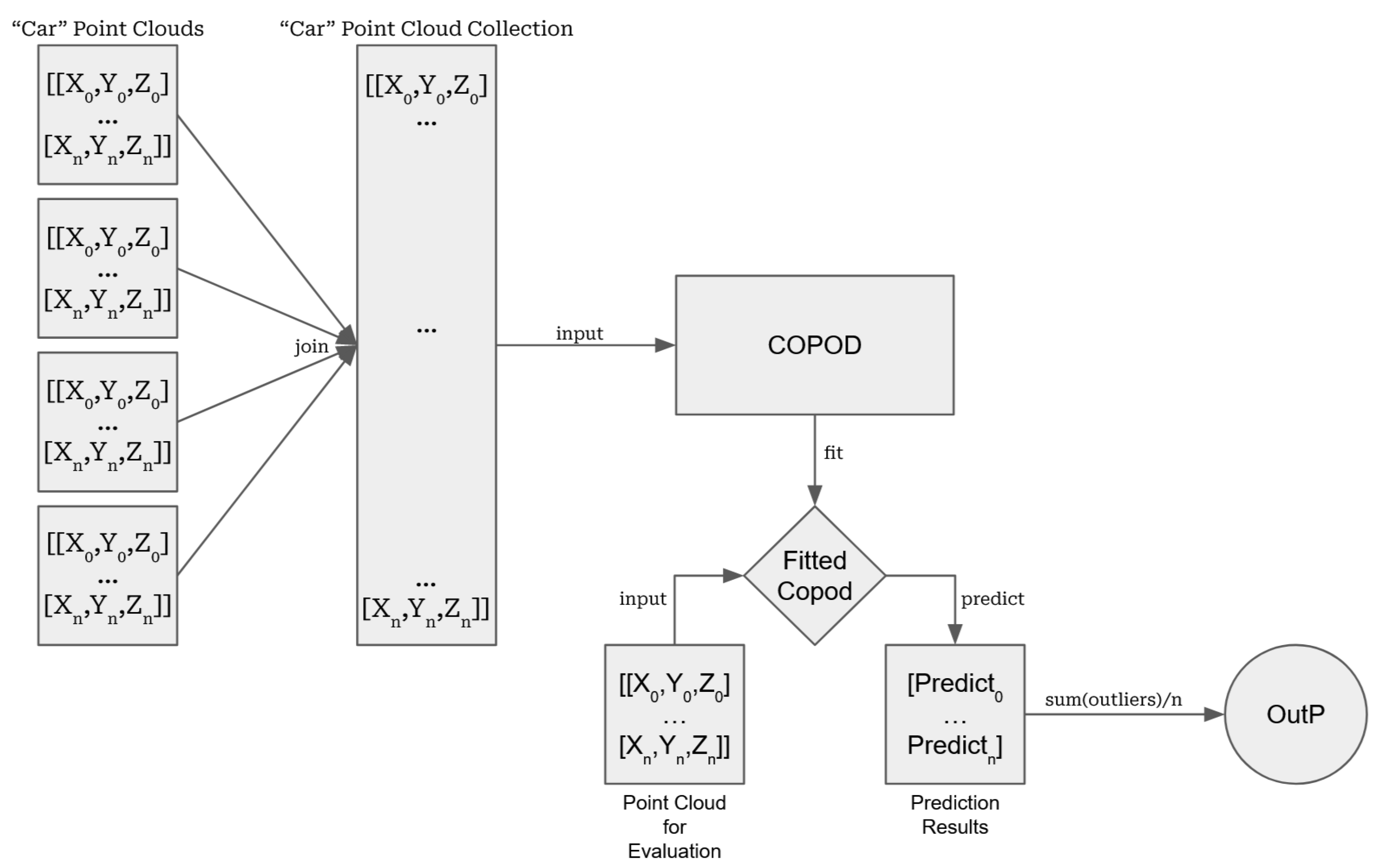
The data treatment process can be seen in
Figure 4. First, we proceeded by extracting the data for a single category in individual NumPy arrays, as outlined previously. These were then gathered into a singular matrix containing as many samples as there were points within all the collected point clouds. Using the
fit function, a copula specific to this category was produced and then used to evaluate single points in one of the three following ways for a single point cloud of size
, where
N denotes the number of points that form that point cloud:
Prediction Method: predicts whether a given point is anomalous or not. The output of this method is a list of size N containing and , with the former denoting outliers and the latter inliers.
Probability Method: predicts the probability of a given point being anomalous. The output of this method is a list of size N containing the computed probabilities and, if requested, a confidence value for the prediction.
Scoring Method: computes the raw anomaly score of a given point. The output of this method is a list of size N containing numbers; those with higher values denote more anomalous points.
Regardless of the method, this algorithm only provides analysis on a per-point basis. As such, a way must be devised to extend these evaluations such that meaningful data on a point-cloud level can be extracted from the individual values. This can be done for each of the above methods as follows:
Prediction: an assessment of the number of outliers present in the cloud is necessary. For this, a simple OutP (Outlier Percentage) is computed by taking the number of outliers and dividing them by the total number of points in the cloud.
Probability: the AAP (Average Anomalous Probability) can be obtained by adding all individual probabilities and using the result to evaluate the whole point cloud.
Scoring: similar to the probability method, an AAS (Average Anomaly Score) can be produced to evaluate the point cloud.
Regardless of the chosen analysis, the resulting output can be equated to a perception algorithm’s confidence score, serving as a measure of the likelihood of any given point cloud belonging (or not) to the category used to fit the copula. When working only with LiDAR data, this method may be implemented alone or supplemented by others; comparing its results to an algorithm’s confidence score provides a way of evaluating the algorithm’s performance.
4. Results
The results presented herein are preliminary, yet show the promising nature of this methodology. They were obtained using four categories: Car, Truck, Pedestrian, and Cyclist. First, the PCs for all bounding boxes present in the 7481 training images were extracted. This extraction was done by identifying every bounding box within a given image corresponding to the targeted category. Next, every point contained within these boxes was collected and the bounding boxes were normalized, with the center serving as the origin point in a Cartesian coordinate system and the corresponding points fitted under it. This allows for dispensing with depth as a parameter, focusing only on how the x, y, and z dimensions of each point relate to the bounding box, resulting in the following sample size for the respective categories:
For the car PCs, approximately 10%, 2841 in total, were extracted for validation. The rest were appended to one another, producing a single array that was then used to train the algorithm and produce a fitted copula. Then, the prediction algorithm was run PC by PC in order to determine whether or not a given point was anomalous. Before moving on to the next cloud, the percentage of anomalous points (OutP) was calculated and stored to produce the graphs shown below.
Before proceeding to a discussion of the specific results, it should be noted that inherent imbalances can be found within most if not all available datasets containing real-world LiDAR data. The prevalence of cars far outweighs that of even pedestrians, and in turn pedestrians often outnumber the remaining categories. This is due to the nature of real-world vehicle diversity and the situations in which these datasets are obtained, which primarily make use of cities and their outskirts. In order to account for this inherent imbalance in the data, there is a need to understand whether it matters for the algorithm’s performance. To find an answer to this question, all categories were truncated to the lowest common denominator by selecting random datapoints from each category.
If these sample populations turn out to be statistically representative of the greater whole, then it is likely that imbalances can be conceivably ignored in the future, as this result indicates that the category used to fit the algorithm contained enough samples for training. Even when statistical significance might have to be proven for each individual dataset, the methodology would remain adequate regardless of any inherent imbalances.
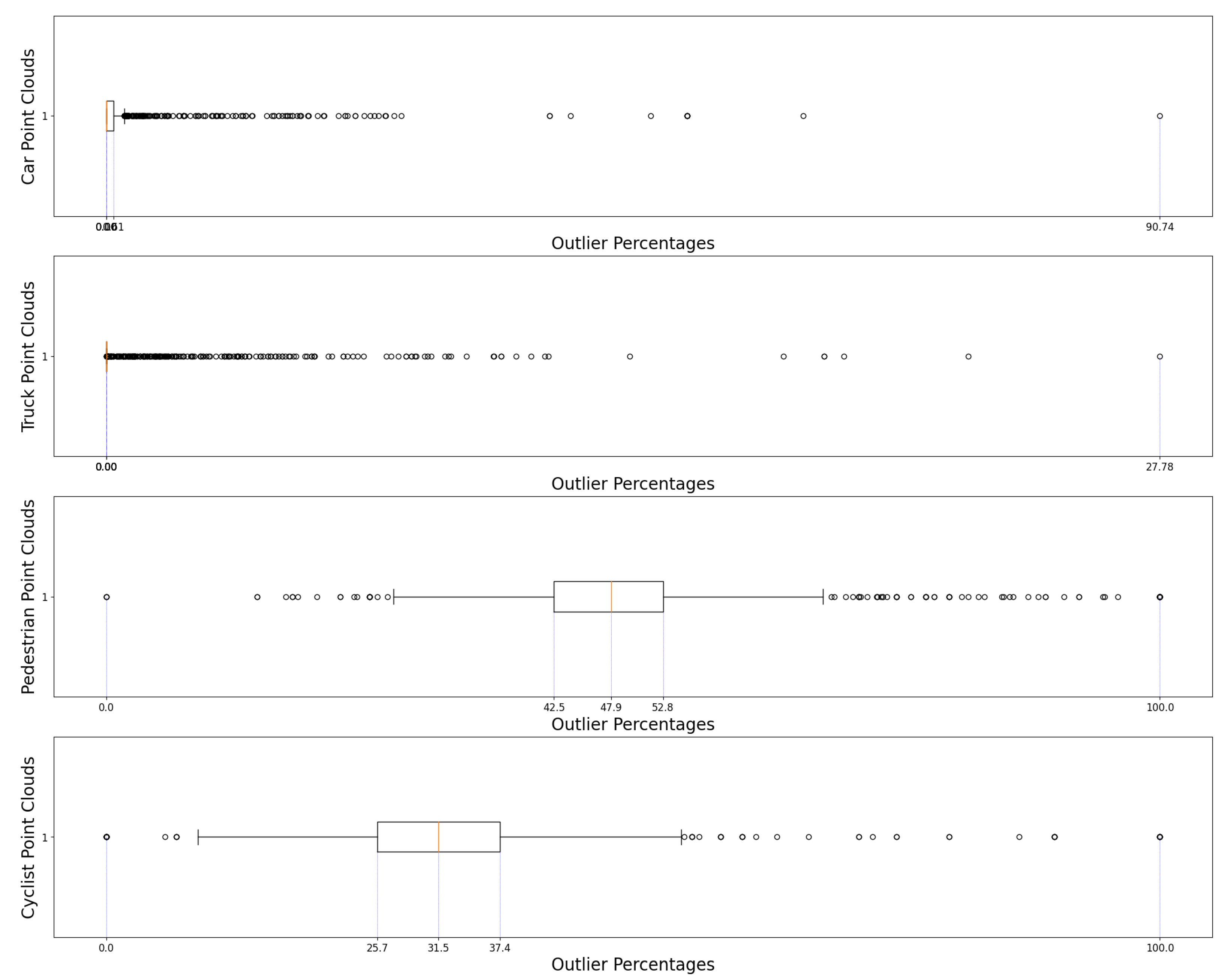
Taking this in consideration, for this first case the amount of samples was truncated to the lowest common denominator, in this case the “truck” category. As this category contained 1084 bounding boxes, the same number of random samples was selected from every other category for comparison via scatter plots, box plots, and relevant statistics such as the quartile, minimum, maximum, and average values for the outlier percentages. The standard deviation and variance were calculated as well. As with the rest of the implementation, these results were obtained via Python using the COPOD algorithm available in pyOD [
22]. Multithreading was not enabled, and the contamination value was set to the default value of 0.1.
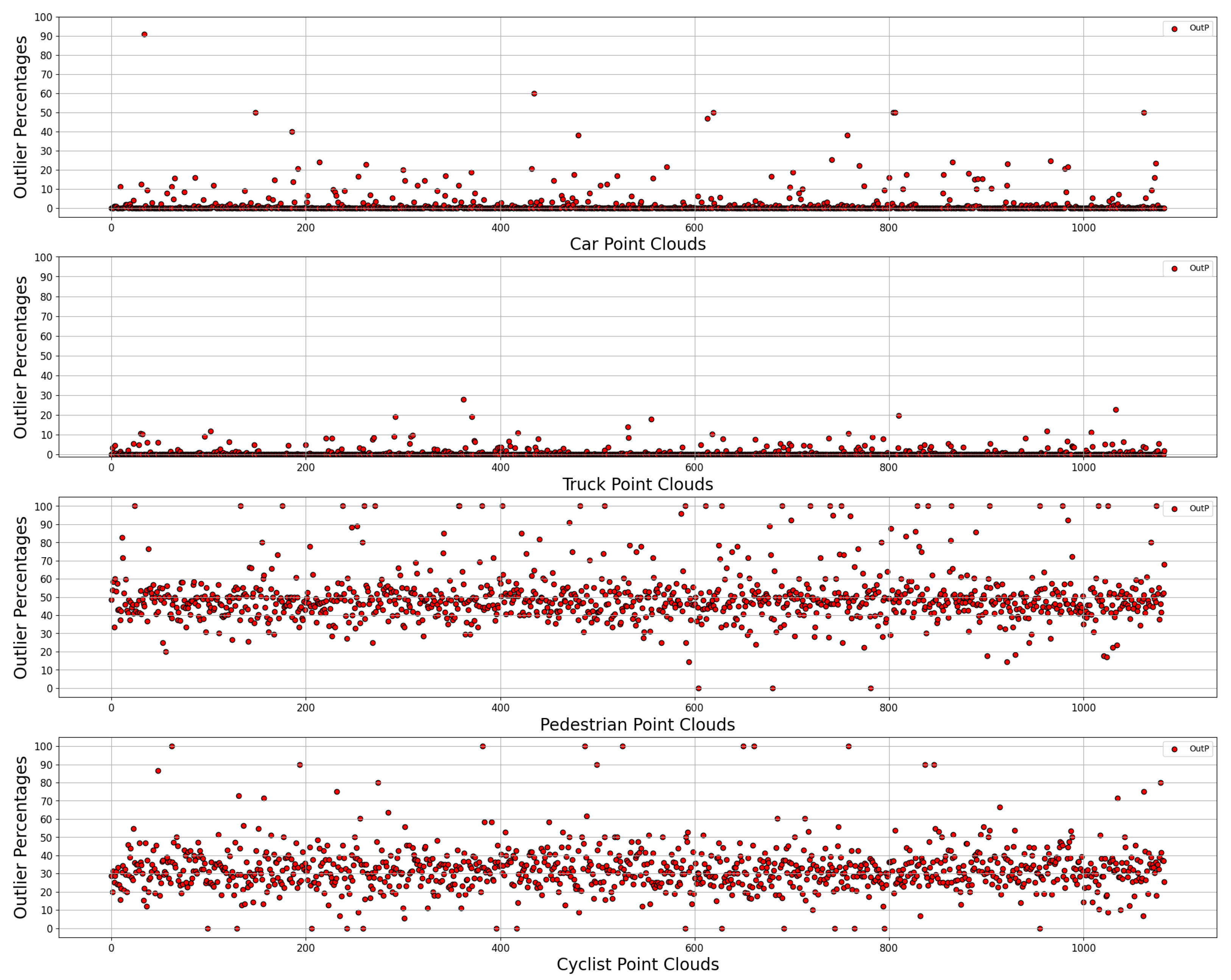
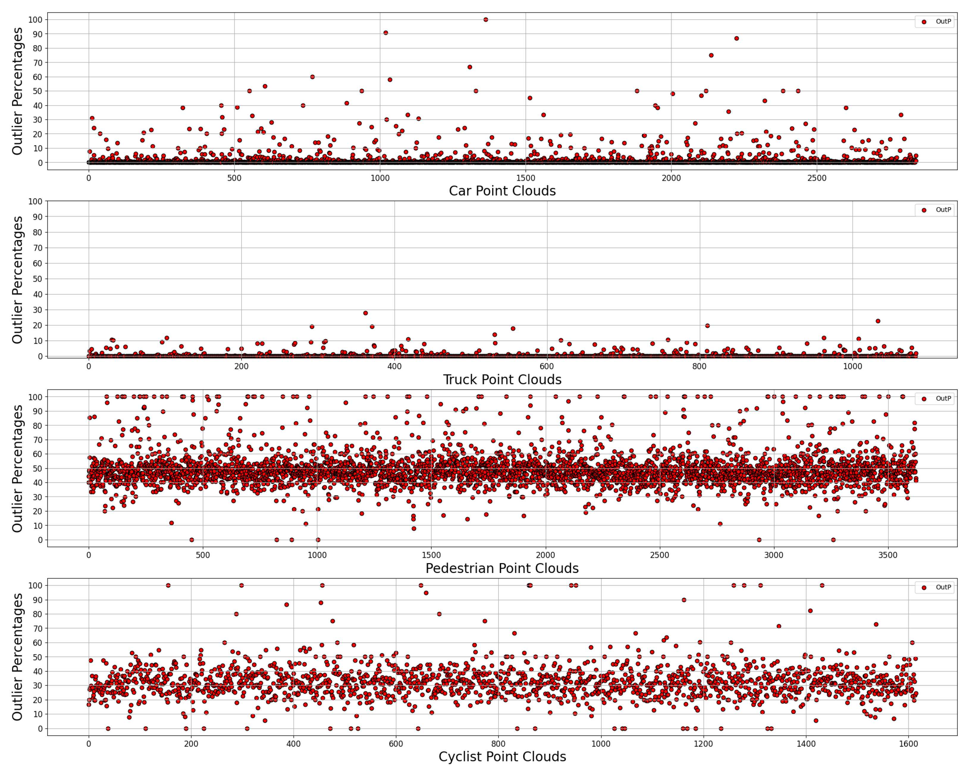
Figure 5 presents an unfiltered showcase of the data, with the following PCs shown from top to bottom: car, truck, pedestrian, cyclist. The graphs show the percentage of points classified as outliers, with the
x-axis identifying the individual PC instances and the
y-axis plotting their respective OutP.
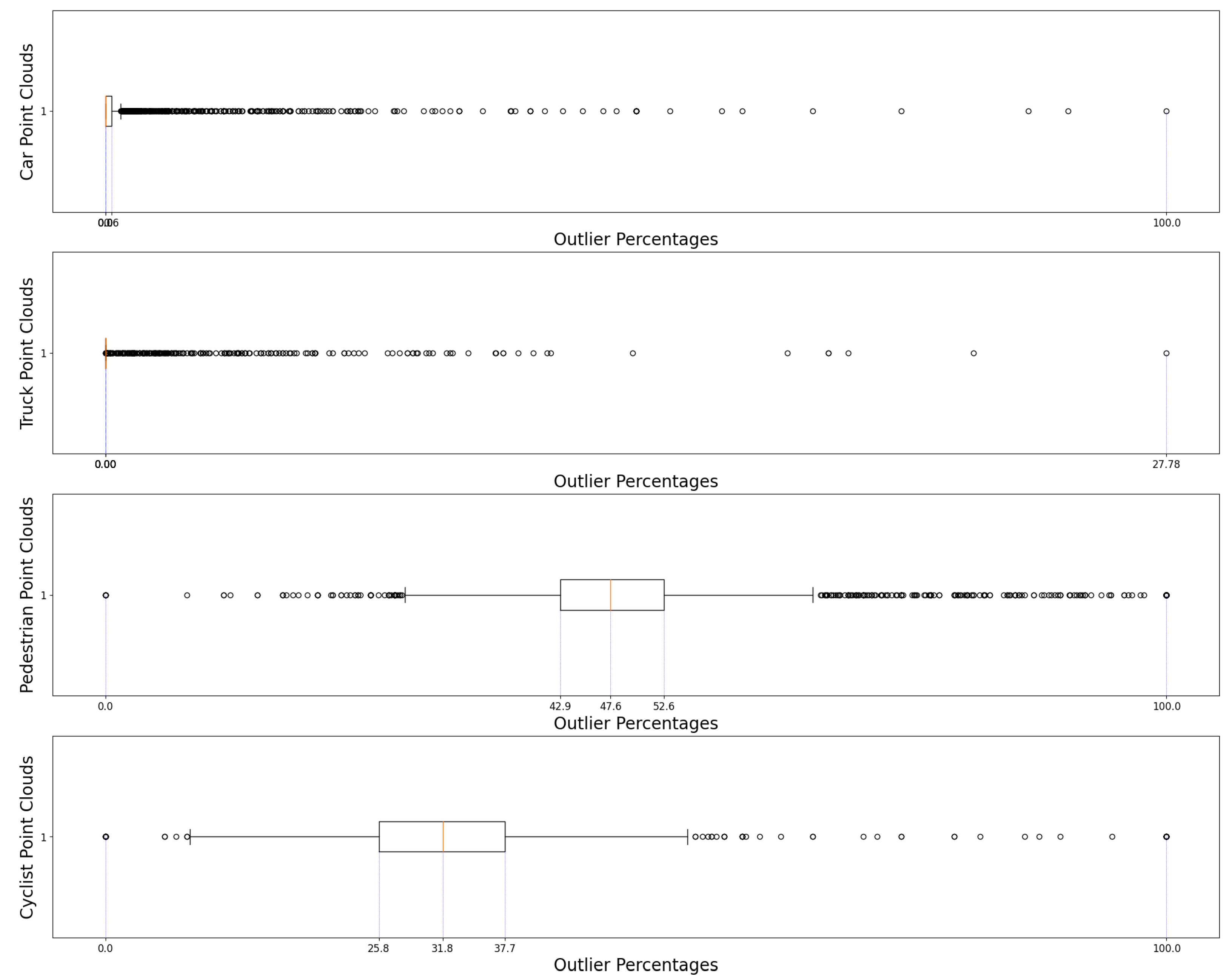
Figure 6 is the associated boxplot, outlining the median(in orange), minimum and maximum values as well as the respective quartiles. This repeates for
Figure 7 and
Figure 8 except without the aforementioned PC truncation.
Through analysis of both figures and
Table 1, it is possible to draw the following conclusions. First, there exists a sizable occurrence of outliers in both the pedestrian and cyclist samples, with the ensuing percentage being considerably higher than that of the other two categories. The same conclusion cannot be extended to the truck point clouds, however; whether this is due to the density of their samples, the shape of the respective LiDAR point clouds, or a mixture of both, they do not appear to be easily distinguishable from car point clouds, and the algorithm fails to provide any meaningful data. The larger size of the objects in the truck category and the higher resolution provided by a larger surface area result in better performance than even the validation samples. Thus, for a given random point cloud it is possible to identify whether it belongs to the “Car–Truck” pair or the “Pedestrian–Cyclist” pair with a fair degree of certainty, in other words, to identify whether or not it is a four-wheeled road vehicle.
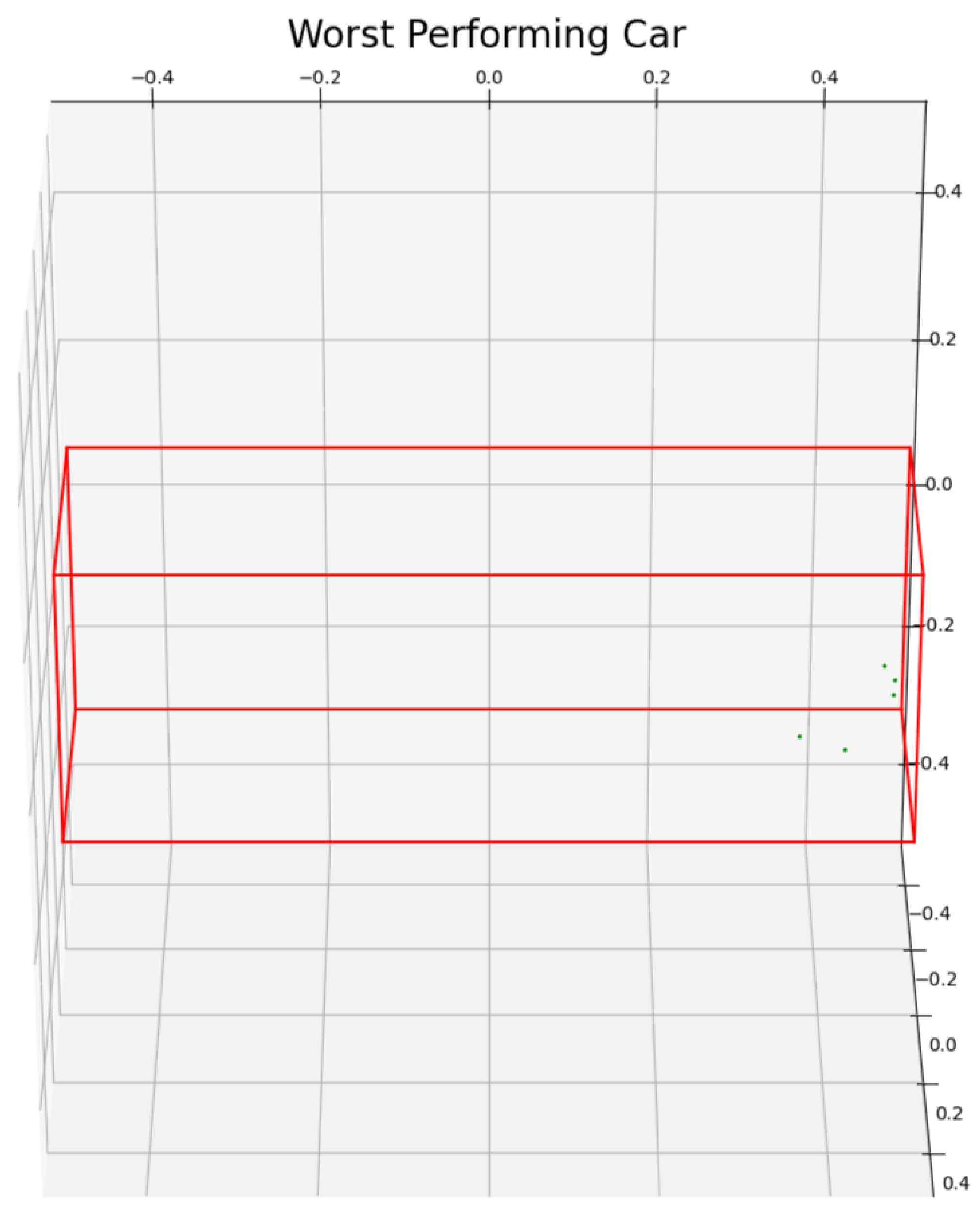
That said, anomalies exist in both the Truck and Car samples. The anomalies derived from point clouds are often scarce, abnormal, or completely lacking in suitable context. As an example, the lowest-performing point cloud for the Car category, with above a 90 percent outlier incidence (
Figure 5), consisted of a handful of random points in space which are entirely disconnected from any manner of shape or object; as can be seen in
Figure 9, these are correctly identified by the algorithm as outliers. A detailed view of the statistical data for this graph can be seen in
Table 1.
Concerning the means of computation, the machine that we used was an ASUS ROG STRIX G173QM personal laptop with a Ryzen 9 5900HX CPU, 16 GB of SODIMM DDR4 RAM, and a core frequency of 3200 MHz. The operating system was Windows 11 using a Jupyter Notebook in VS Code. Each batch of 100 frames contained a varied amount of data and was processed in 80 to 100 min, with only occasional variance in particularly sparse frame batches. These results were obtained without multithreading enabled due to the use of a personal computer and the need for enough resources to be kept available for regular use.
After the preliminary tests were concluded, the relevant sample (the pedestrian PCs) was scaled to include all of the available data for that category, making for a total of 3623. The goal was to determine whether this trend continued, and if it did to discern whether the first results were statistically significant, in which case it could be fairly assumed that the same pattern would be present in the car samples.
Figure 7 provides a comparison between the results obtained considering the entirety of the data without any sample size truncation. The data appear to accurately portray the expected distribution obtained with the truncated sample size. Notably, the pedestrian point clouds demonstrate a large concentration of points gravitating around the 50% OutP value. An incidence of samples with more than 60% OutP suggests that the algorithm can identify anomalous points that do not belong to the fitted copula describing an idealized Car PC. This ability enables the algorithm to indicate possible points of contention within the Car category as well as similar ones such as the Truck category while correctly identifying most pedestrians as falling outside the expected parameters, with only a few exceptions. Furthermore, the cyclist samples follow a similar, albeit less drastic pattern to the pedestrian category, which further serves as an indication of the algorithm’s ability to distinguish between PCs.
The aforementioned exceptions can be denoted as Car samples with abnormally high scores and non-Car or Truck samples with abnormally low scores, anomalies which can be explained through the quality and density of the point clouds associated with these samples. An example of this is shown in
Figure 9, where the reason behind the high OutP score is made apparent through the lack of extractable context given such a sparse and insignificant point cloud. A detailed look into the statistics is provided in
Table 2.
Comparisons with other methods that operate within the same area are hard to draw. As previously noted, the amount of research within the realm of data validation and evaluation regarding solely LIDAR data is scarce. Furthermore, most methods rely on the usage of machine learning algorithms, making direct comparisons of each approach limited. At most, the confidence score provided by an object detection algorithm can be compared to the outlier score produced by the same algorithm, or the categorical assertions of the former score can be compared to the statistics of the latter. Thus, most of the high-fidelity algorithms used for machine learning purposes are either multimodal or rely mostly on traditional cameras, making it difficult to obtain fair comparisons.
5. Conclusions and Future Work
Solutions for advanced driver-assistance systems and autonomous driving are currently being developed to improve driving comfort and safety in newly developed vehicles and next-generation automated and autonomous vehicles. While these systems resort to LiDAR technology to capture three-dimensional data, it is the underlying perception layer that interprets and understands the scanned surroundings. Recently reported accidents involving autonomous vehicles have often been shown in studies to be due to failures within the perception layer. As driving environments are often uncontrolled and complex, there are many factors which may contribute to data corruption, such as LiDAR laser beam divergence from backscattering, adverse weather conditions, the state of the road, sensor performance degradation, and varied sources of external interference.
Robust and accurate LiDAR perception algorithms must be produced in order to achieve safety in assisted and automated driving systems. Part of this process lies in creating robust and thorough methodologies to evaluate their performance and guarantee the integrity of training data. This work presents results of a method proposed for this purpose which is capable of detecting anomalous patterns in LiDAR data. The results obtained through the proposed method can be used to complement other performance evaluations and metrics. This method relies on the Copula-based Outlier Detection algorithm (COPOD) to identify outliers in a given object category. Three types of metrics are used: those that predict whether or not a given point is anomalous; those that predict the probability of a point being anomalous; and those used to compute the raw anomaly score of a given point. The proposed method can be used to evaluate an algorithm’s confidence score. In addition, it shows the potential to identify the impact that adverse conditions may have on LiDAR data, as adverse conditions can increase data scattering. Finally, it can detect cases in which the data may be insufficient or otherwise unusable.
Further work is being carried out to include other datasets in an effort to better study the manner in which LiDAR resolution and point cloud density impact algorithm performance. This primarily involves including data on the intensity of the LiDAR captured laser beam and the use of datasets containing different weather conditions. Another prospect is to combine the results of the proposed methodology with other metrics, such as intersection-over-union, in order to exclude point clouds which contain only the silhouette or outline of a car as opposed to an actual car. The ultimate objective of this future research is to generate key performance indicators that can be used to evaluate perception algorithms.


