Soil Salinity Estimation in Cotton Fields in Arid Regions Based on Multi-Granularity Spectral Segmentation (MGSS)

Abstract

Soil salinization seriously threatens agricultural production and ecological environments in arid areas. The accurate and rapid monitoring of soil salinity and its spatial variability is of great significance for the amelioration of saline soils. In this study, 191 soil samples were collected from cotton fields in southern Xinjiang, China, to obtain spectral reflectance and electrical conductivity (EC) indoors. Then, multi-granularity spectral segmentation (MGSS) and seven conventional spectral preprocessing methods were employed to preprocess the spectral data, followed by the construction of partial least squares regression (PLSR) models for soil EC estimation. Finally, the performance of the models was compared. The results showed that compared with conventional spectral preprocessing methods, MGSS could greatly improve the correlation between spectrum and soil EC, extract the weak spectral information of soil EC, and expand the spectral utilization range. The model validation results showed that the PLSR model based on the second-order derivative (2nd-der-PLSR) had the highest estimation accuracy among the models constructed by conventional methods. However, the PLSR model based on MGSS (MGSS-PLSR) had the highest estimation accuracy among all models, with R_p² (0.901) and RPD (3.080) being 0.151 and 1.302 higher than those of the 2nd-der-PLSR model, respectively, and nRMSEP (5.857%) being 4.29% lower than that of the 2nd-der-PLSR model. The reason for the high accuracy of the MGSS-PLSR model is as follows: In the continuous segmentation of the raw spectrum by MGSS, the bands with strong and weak correlations with respect to soil EC were concentrated during low granularity segmentation. With the increase in granularity level, the spectral features decreased and were distributed discretely. In addition, the locations of spectral features were also different at different granularity levels. Therefore, the spectral features of soil EC can be effectively extracted by the MGSS, which significantly improves the spectral estimation accuracy of soil salinity. This study provides a new technical means for soil salinity estimation in arid areas.

1. Introduction

Soil salinization is a main cause of land degradation and a major threat to sustainable agricultural development in arid areas [1]. It not only causes a decline in soil quality, crop yield loss, and land desertification [2] but also impacts ecosystem functions and biological diversity [3]. Over the past 20 years, about one-third of farmlands has been salinized [4], and global salinized soil reaches about 9.55 × 10⁸ hm². A study has shown that the area of salinized soil in China is about 3.6 × 10⁷ hm², accounting for 6.62% of the total arable land [5]. Xinjiang is located in northwest China. Due to the influences of natural factors such as low precipitation, large evaporation, and high groundwater level [6], Xinjiang has the largest area of salinized soil (1.26 × 10⁶ hm²) in China [7].

The rapid and accurate estimation of soil salinity is of great importance for the amelioration of saline soils. Conventional soil salinity measurement methods are time-consuming, labor-intensive, and difficult to use for large-scale quantitative assessments [8]. However, remote sensing technology can quickly and non-destructively obtain soil information. Therefore, it has been widely used in soil salinity estimation [9]. At present, many scholars have adopted different spectral preprocessing methods to improve the accuracy of soil salinity spectral estimation. For example, Fu et al. [10] performed root mean square ($\sqrt{\mathrm{R}}$), reciprocal (1/R), inverse logarithmic (log(1/R)), logarithmic, and logarithmic reciprocal preprocessing after Savitzky–Golay (SG) convolution smoothing on the raw spectra and found that the model accuracy constructed based on SG smoothing and 1/R preprocessing was the highest. Shi et al. [11] performed logarithmic, exponential, and square root (R^1/2) preprocessing on raw spectral data to construct spectral indices and found that preprocessing obviously improved the soil salinity estimation accuracy compared with the raw spectra data, especially R^1/2 preprocessing. Wang and Li [12] constructed support vector regression (SVR) models after preprocessing raw spectral data using average reflectance (R), the logarithm of the reciprocal of R, and the continuum removal of reflectance (Rcr), and they found that the R-based and Rcr-based SVR model had the highest accuracy in estimating soil Cl⁻ and K⁺ content, respectively. In addition, wavelet transform (WT), fractional differentiation (FD), and empirical mode decomposition [13,14] have also been used to preprocess raw spectral data and achieved high estimation accuracy.

However, the spectra of some soil parameters such as soil salinity usually overlap with those of other parameters such as soil nutrients and heavy metals [15]. Although the above spectral preprocessing methods can improve the estimation accuracy to a certain extent [16,17], weak and overlapping spectra cannot be extracted after preprocessing, leading to a loss of some spectral features [18]. In addition, wavelet transform (WT), fractional differentiation (FD), and empirical mode decomposition can only extract floating-point values, which increases the data volume and data processing complexity and makes them difficult to use for large-scale parameter retrieval [19]. Therefore, Kang and Zhang [20] proposed MGSS to segment the spectrum with the idea of circular cutting and to extract multi-granularity spectral features for quantitative inversion. MGSS could reduce the cost of data storage and transmission, improve computational efficiency via data simplification, and extract weak spectral information. In particular, it can extract the overlap and full-band spectral information. However, at present, the comparison of the soil salinity spectral estimation accuracy based on MGSS and other commonly used preprocessing methods has not been performed.

Cotton is a major cash crop in Xinjiang [21]. In 2021, Xinjiang planted more than 2.6 million hectares of cotton, and Xinjiang’s cotton output (5.13 million tons) accounted for one-fifth of the world’s cotton production [22]. However, in recent years, flood irrigation has led to increased soil salinization in Xinjiang [23,24]. About 30% of cotton crops in Xinjiang face saline stress. High soil salinity seriously restricts cotton growth, especially at the seedling stage [25], and leads to great yield losses [26]. Therefore, the amelioration of saline soils is very important for sustainable agricultural development in Xinjiang. The accurate monitoring of soil salinity is a prerequisite for saline soil amelioration [27]. Therefore, in this study, MGSS was employed to process the raw spectral data of soil electrical conductivity (EC) for soil salinity estimation, and the estimation accuracy based on MGSS was compared with that based on seven conventional spectral preprocessing methods. The objectives were to (1) determine the feasibility of MGSS in soil salinity estimation and (2) compare the estimation accuracy based on the MGSS with that based on conventional spectral preprocessing methods. This study will provide a new technical means for soil salinity estimation and contribute to the amelioration of saline soils and crop yield increase in arid areas.

2. Materials and Methods

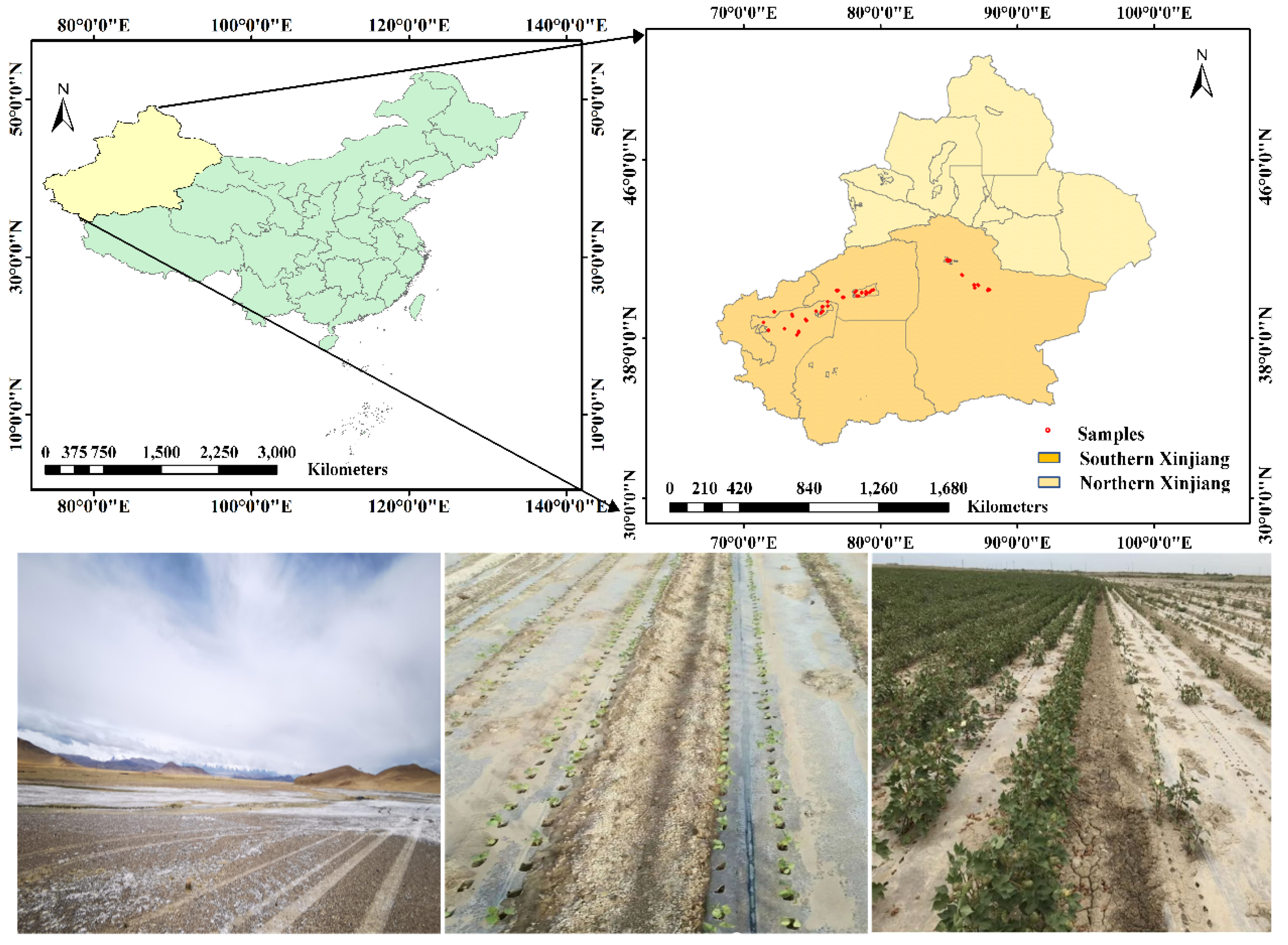
2.1. Study Site

Southern Xinjiang, a main cotton production base of China [28], is mainly a large closed intermountain basin (Tarim Basin, a.s.l. 1000~2000 m). Geologically, it is a stable block restricted by many deep and large surrounding faults. The terrain of the basin is high in the west and low in the east. The soil and rock minerals are mainly physically weathered, forming a coarser parent material. Due to differences in latitude and terrain, the types of landforms are very complex, resulting in different soil types [29]. The parent materials of plain soil mainly include alluvial deposits and loess. The soil types are mainly desert soil, meadow soil, fluvo-aquic soil, saline soil, and aeolian sandy soil. Soil texture is mainly silty loam and sandy loam [30]. In this study, Korla, Aksu, and Kashgar in southern Xinjiang were selected. These regions have a temperate continental climate with long sunshine duration, low rainfall, high evaporation, and large day/night temperature difference. The annual precipitation is 25~100 mm. The accumulated temperature is more than 3500 °C. The frost-free period is 200~220 days [30].

2.2. Data Collection

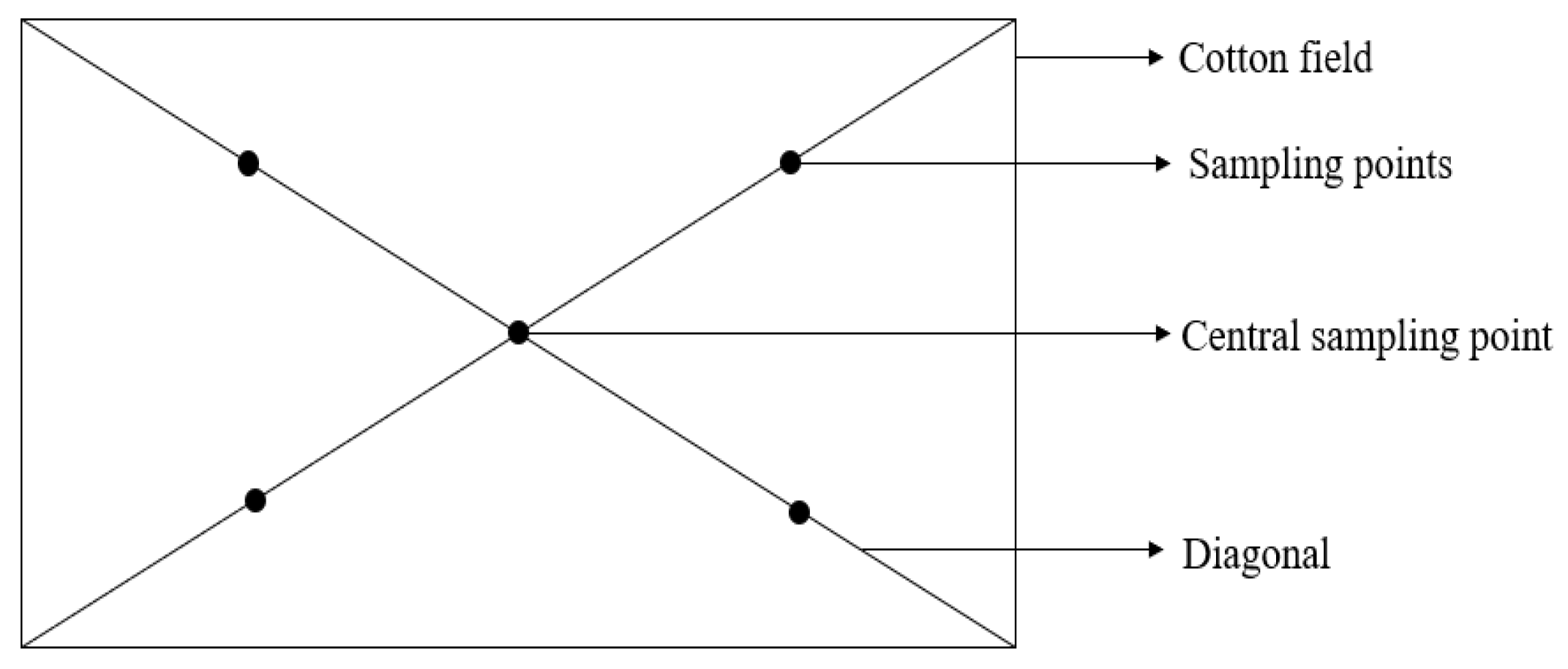
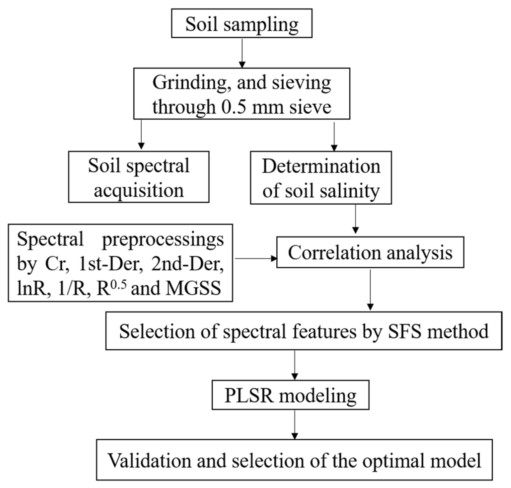
2.2.1. Soil Sampling

From 22 September to 8 October 2020, cotton fields greater than 33.3 × 10³ m² were selected in the study area (Figure 1), and five points were selected in each field along the diagonals for soil sampling. Specifically, firstly, the two diagonal lines of a cotton field were drawn. Then, the intersection (center point) of the two diagonal lines was selected as a sampling point. After that, four points were selected as the other four sampling points at half the distance from the four corners of the cotton field to the center point (Figure 2). The sampling points were positioned using a GPS device (Garmin eTrex vistah, Taiwan, China). After removing plant roots, stones, and other impurities, the 0~20 cm soil layer was collected vertically using an earth-boring auger [31]. Five soil samples were collected in each field, mixed, sealed in polyethylene bags, and brought back to the lab. Soil samples were dried, ground, and passed through a 0.5 mm sieve [32]. After that, each soil sample was divided into two parts: one for measuring soil EC and the other for soil spectral acquisition.

2.2.2. Determination of Soil Salinity

Five grams of soil sample and 25 mL of distilled water were mixed in a conical flask and shaken for 30 min [33]. Then, the mixture was filtered, followed by the measurement of soil EC using a conductivity meter (S230, Mettler Toledo Instrument Co., Ltd., Shanghai, China). Each sample was measured three times, and the average value was calculated.

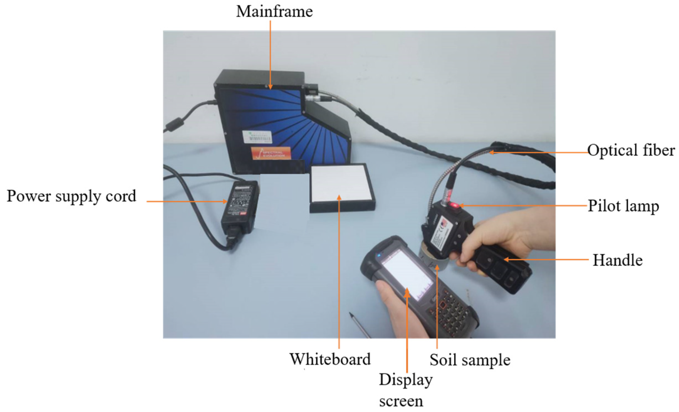
2.2.3. Spectral Acquisition

Because soil salinity and soil EC have a positive correlation and soil EC has a more prominent spectral response than soil salinity, the spectral information of soil EC has been widely used to estimate soil salinity [34]. In this study, the ASD Field Spec Pro FR spectrometer (Boulder, CO, USA) was used to collect the spectral data of soil samples in the lab. The wavelength range was 350~2500 nm, and the spectral resolutions at 350~1000 nm and 1000~2500 nm were 3 and 10 nm, respectively. The spectral sampling interval was 1 nm.

The spectral acquisition details were as follows: Firstly, the soil sample was placed in an aluminum box (5 cm in radius and 1.5 cm in depth). Then, the optical fiber was connected to the handle. After that, the switch on the handle and the APP configured for the instrument were connected via Bluetooth, and the number of spectral curves was set to 5. After half an hour, the four walls of the luminous port at the end of the handle came into direct contact with the soil surface, forming a confined space where all light hits the soil sample. The reflectance spectra of the soil samples were received by the probe (Figure 3). The device was calibrated every ten minutes during measurements to prevent sensor drift and a change in incidence angle. The spectral acquisition was performed three times for each soil sample, and the average value was used for analysis.

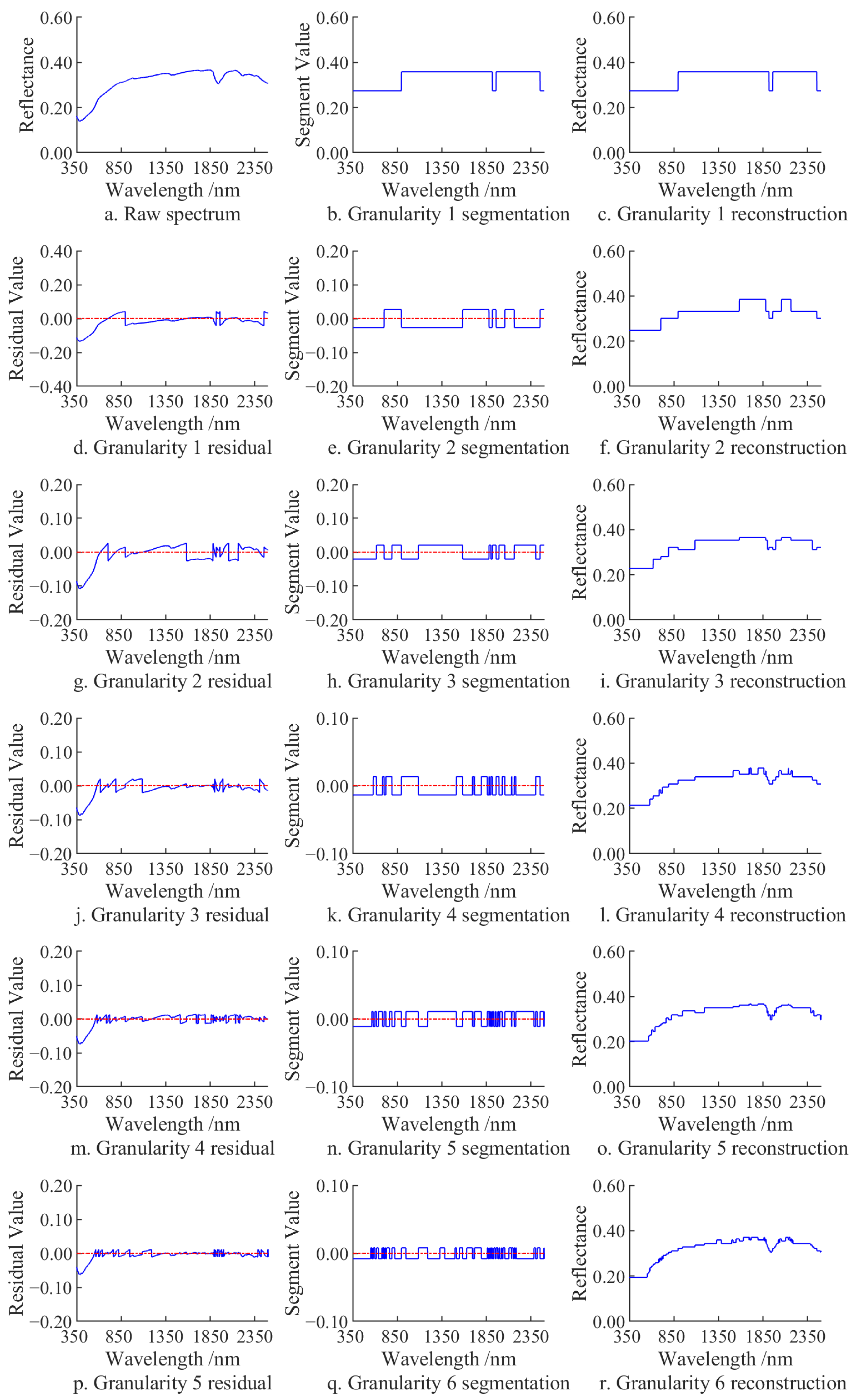
2.2.4. Spectral Data Preprocessing

MGSS is developed on the basis of spectral high-order binary coding, which transforms the data storage format to realize data compression and restoration (i.e., transforming 16-bit data into 12-bit data) [35]. Compared with high-order binary coding, MGSS could effectively reduce the loss of spectral details in the conversion process. The essence of MGSS is a continuous operation of de-averaging the spectrum. This could highlight weak spectral information. It is assumed that the spectral vector can be approximated by the sum of the products of the M-order segment value (M > 0) and its coefficient, and the residual error decreases with an increase in M:

$$\mathrm{V}=\sum _{\mathrm{i}=1}^{\mathrm{M}}{\mathsf{\beta }}_{\mathrm{i}}{\mathrm{H}}_{\mathrm{i}}+{\mathrm{R}}_{\mathrm{M}}\left(\mathrm{V}\right)\approx \sum _{\mathrm{i}}^{\mathrm{M}}{\mathsf{\beta }}_{\mathrm{i}}{\mathrm{H}}_{\mathrm{i}}$$

(1)

where H_i is the ith order segment value of the spectral vector $\mathrm{V};{\mathrm{H}}_{\mathrm{i}}\in {\left\{-1,1\right\}}^{\mathrm{M}}$; β_i is the coefficient of H_i, β_i > 0; and RM(V) is the residual vector of the M-order quantized estimation of V.

The analytical solution of Formula (1) can be obtained by carrying out convex optimization:

$$\left\{\begin{array}{c}{\mathsf{\beta }}_{\mathrm{i}}=\frac{1}{\mathrm{N}}|\left|{\mathrm{R}}_{\mathrm{i}-1}\left(\mathrm{V}\right)\right||{\mathrm{L}}_1\\ {\mathrm{H}}_{\mathrm{i}}=\mathrm{sign}({\mathrm{R}}_{\mathrm{i}-1}(\mathrm{V}))\end{array}\right.$$

(2)

where i = 1, 2, …, M; N is the number of bands; ${\mathrm{L}}_1$ represents 1-norm; and sign() is a sign function. When T ≥ 0, sign(T) = 1, and when T < 0, sign(T) = −1.

Then, the spectral segmentation can be summarized as follows:

$$\left\{\begin{array}{c}S{\mathrm{F}}_{\mathrm{i}}=S{\mathrm{F}}_{\mathrm{i}-1}-S{\mathrm{L}}_{\mathrm{i}}\\ S{\mathrm{L}}_{\mathrm{i}}={\mathsf{\beta }}_{\mathrm{i}}\times {\mathrm{H}}_{\mathrm{i}}\\ {\mathrm{A}\mathrm{S}}_{\mathrm{i}}={\sum }_{\mathrm{t}=1}^{\mathrm{i}}\mathrm{S}{\mathrm{L}}_{\mathrm{t}}\end{array}\right.$$

(3)

where SF_i is the spectral feature (i.e., residual feature) obtained at the ith spectral segmentation, that is, the raw hyperspectral data are continuously deaveraged to highlight weak and detailed spectral information. SL_i is the line for segmenting at the ith segmentation, and AS_i is the approximate spectrum after ith segmentation, which can achieve data compression.

The following (Figure 4) is an example of MGSS. Figure 4a shows the hyperspectral curves of soil samples, the SF₀ is itself. Figure 4b shows the SL₁ (SL₁ = β₁ × H₁) for the 1st segmentation, and the spectral feature at the 1st segmentation can be obtained by SF₁ = SF₀ − SL₁. Figure 4c shows the approximate spectrum of the raw spectrum after the 1st segmentation. According to Formula (2), β₂ and H₂ can be calculated, and then SL₂ is calculated (SL₂ = β₂ × H₂), after which SF₂ can be obtained. SL₃~SL₃₀ can be extracted by repeating the above process.

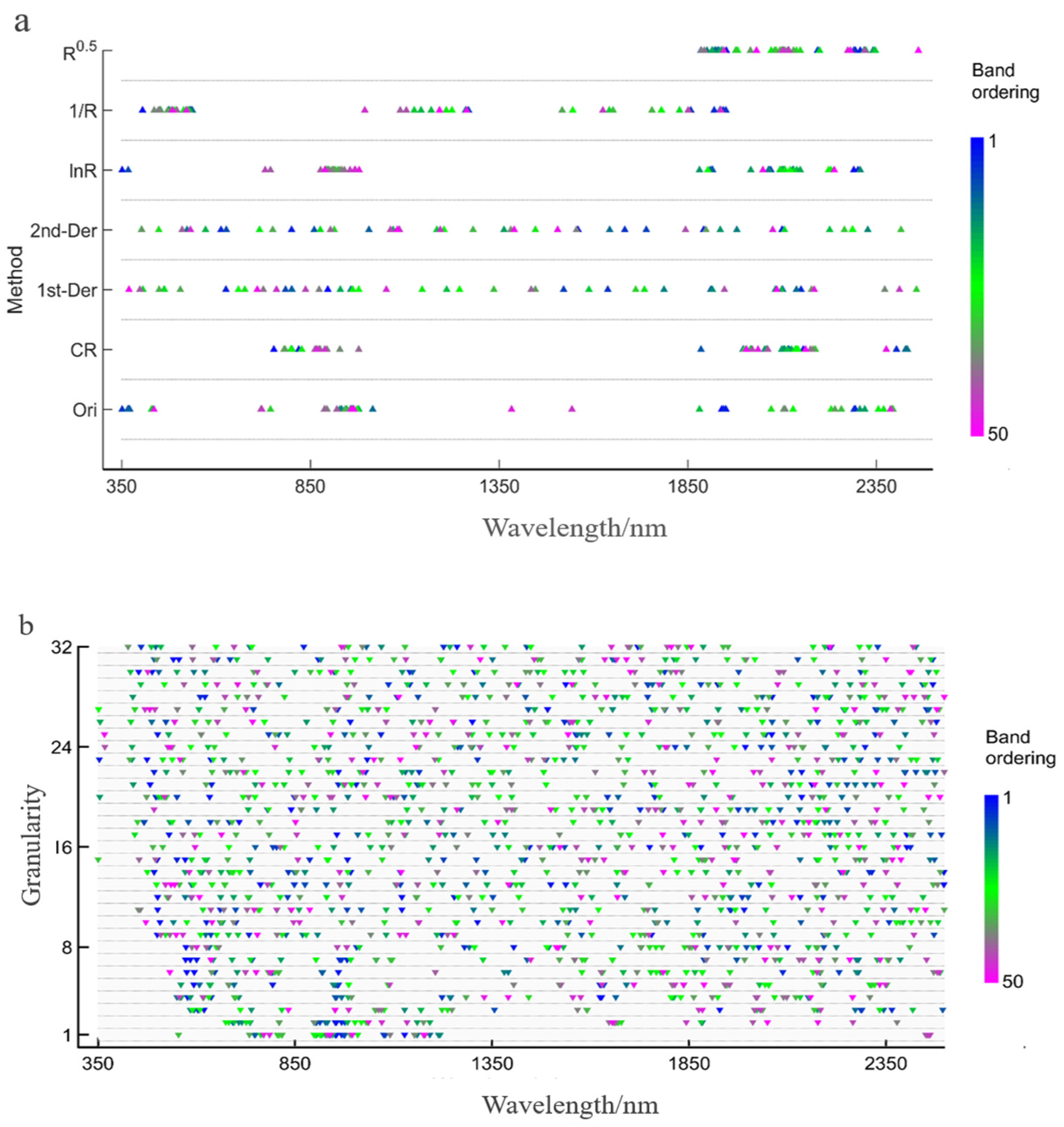
2.3. Selection of Spectral Features

The number of spectral bands and spectral features obtained increased exponentially with the increase in granularity. Therefore, it is necessary to select the optimal spectral features at each granularity after segmentation to improve the inversion accuracy. In this study, the sequential forward selection (SFS) method [36] was used to select spectral features after spectral preprocessing using seven conventional methods and MGSS. That is, the optimal band was selected from the preprocessed spectral data for multiple cycles and added to the spectral feature set until the spectral feature set can achieve the highest soil EC estimation accuracy.

To facilitate comparisons between conventional methods and MGSS, the same number of spectral features (50) was selected by SFS for each conventional method and each granularity in MGSS. Specifically, spectral data were normalized and standardized. Then, an empty feature set ${\mathrm{y}}_0=\left\{\mathrm{\varnothing }\right\}$ was constructed. After that, a feature, $\mathrm{x}$, was selected to make $\mathrm{J}({\mathrm{y}}_{\mathrm{k}}+\mathrm{x})$ the optimal, that is, ${\mathrm{x}}^{+}=\mathrm{a}\mathrm{r}\mathrm{g}\underset{\mathrm{x}\in {\mathrm{y}}_{\mathrm{k}}}{\max }\left[\mathrm{J}({\mathrm{y}}_{\mathrm{k}}+\mathrm{x})\right]$, and ${\mathrm{x}}^{+}$ was added to the feature subset $\mathrm{y}$ (${\mathrm{y}}_{\mathrm{k}+1}={\mathrm{y}}_{\mathrm{k}}+{\mathrm{x}}^{+},\mathrm{k}=\mathrm{k}+1)$. Finally, the third step was repeated multiple times until the combined performance of feature set $\mathrm{x}$ was satisfactory.

PLSR could reduce data dimension and collinearity between independent variables, eliminate redundancy, and maintain the interpretation ability of principal components to output variables [37]. In this study, the PLSR estimation model was constructed for soil salinity spectral estimation. The entire dataset (191) was divided into a calibration set (115) and a validation set (76) at a 3:2 ratio (

Table 1. Electrical conductivity of soil samples.

Dataset	No.	Max.	Min.	Mean	Std	Cv	Kurtosis	Skewness
Full dataset	191	2.37	0.06	0.73	0.49	0.67	3.57	0.89
Calibration set	115	2.37	0.06	0.81	0.52	0.63	2.98	0.66
Validation set	76	2.33	0.07	0.60	0.42	0.70	5.49	1.28

) using the Kennard–Stone (K-S) method [7] to ensure generalization and the robustness of the model [38]. The mean values of the entire dataset, calibration set, and validation set were 0.73, 0.81, and 0.60, respectively, but maximums, minimums, standard deviations, and coefficients of variation were very close. This indicates that the entire dataset, calibration set, and validation set have a high degree of similarity and consistency. To avoid overfitting, the optimal number of latent variables (LVs) was determined by minimizing the root mean square error of cross validation based on the calibration set [36].

In this study, the coefficient of determination ((R²) (Equation (4)), normalized root mean square errors ((nRMSE) (Equation (5)), and the ratio of performance to deviation ((RPD) (Equation (6)) were used to evaluate the accuracy of the models constructed based on different preprocessing methods [7]. The root mean square error (RMSE) and nRMSE were calculated according to Equations (5) and (7), respectively, and the RPD was calculated based on the standard deviation ((SD) (Equation (8)) and RMSE. These indicators were further refined into the nRMSE of calibration (nRMSEC), R² of calibration (R_c²), nRMSEP (nRMSE of validation), R_p² (R² of validation), and RPD (RPD of validation). Generally, the models with high accuracy have high R_c², R_p², and RPD and low nRMSEC and nRMSEP. In addition, the smaller the difference between nRMSEC and nRMSEP, the more stable the estimation accuracy of the model [39]. R_c² and nRMSEC were calculated based on the optimal number of LVs:

$${\mathrm{R}}^2=\frac{\sum _{\mathrm{i}=1}^{\mathrm{n}}{({\mathrm{X}}_{\mathrm{i}}-\stackrel{-}{\mathrm{X}})}^2{({\mathrm{Y}}_{\mathrm{i}}-\stackrel{-}{\mathrm{Y}})}^2}{\sum _{\mathrm{i}=1}^{\mathrm{n}}{({\mathrm{X}}_{\mathrm{i}}-\stackrel{-}{\mathrm{X}})}^2\sum _{\mathrm{i}=1}^{\mathrm{n}}{({\mathrm{Y}}_{\mathrm{i}}-\stackrel{-}{\mathrm{Y}})}^2}$$

(4)

$$\mathrm{nRMSE}=\frac{\mathrm{RMSE}}{\mathrm{Max}-\mathrm{Min}}$$

(5)

$$\mathrm{RPD}=\frac{\mathrm{SD}}{\mathrm{RMSE}}$$

(6)

$$\mathrm{RMSE}=\sqrt{\frac{\sum _{\mathrm{i}=1}^{\mathrm{n}}{({\mathrm{X}}_{\mathrm{i}}-{\mathrm{Y}}_{\mathrm{i}})}^2}{\mathrm{n}}}$$

(7)

$$\mathrm{SD}=\sqrt{\frac{\sum _{\mathrm{i}=1}^{\mathrm{n}}{({\mathrm{X}}_{\mathrm{i}}-\stackrel{-}{\mathrm{X}})}^2}{\mathrm{n}}}$$

(8)

where i represents the data of sampling point i, ${\mathrm{X}}_{\mathrm{i}}$ is the measured value of soil EC at sampling point i, Y_i is the predicted value of soil EC at sampling point i, $\stackrel{-}{\mathrm{X}}$ is the average value of the measured values of soil EC, $\stackrel{-}{\mathrm{Y}}$ is the average value of the predicted values of soil EC, $\mathrm{n}$ is the total number of samples, and Max and Min are the maximum and minimum values of the sample set, respectively.

2.4. Model Validation

The PLSR model constructed based on the calibration set was used to estimate the soil salinity of sampling points in the validation set, and the R_p², nRMSEP, and RPD were calculated to evaluate the model estimation accuracy. The detailed modeling process is shown in Figure 5.

3. Results

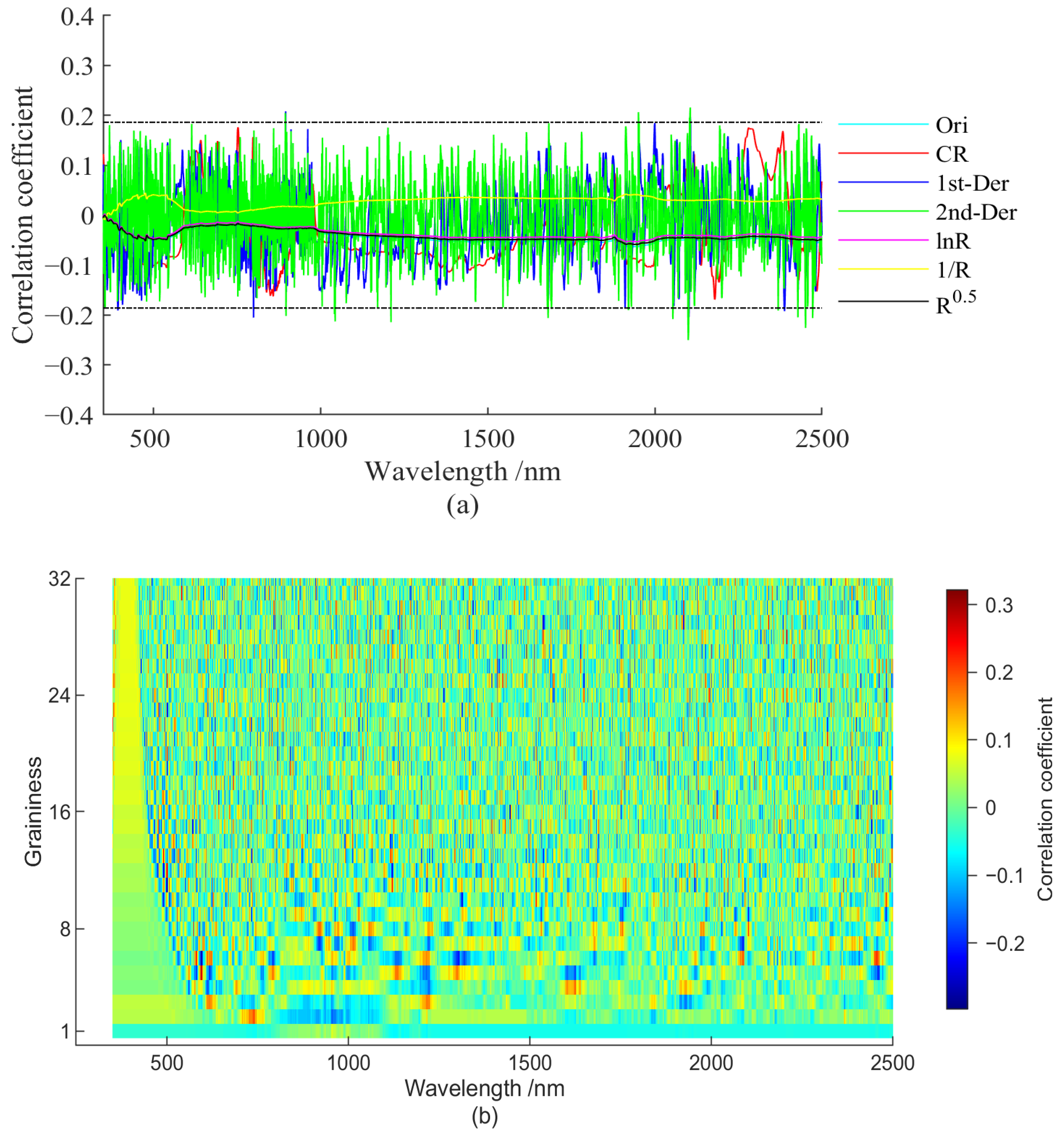
3.1. Spectral Features of Soil EC

In this study, conventional preprocessing methods include original (Ori), natural logarithm of R (lnR), 1/R, root mean square of R (R^0.5), the first derivative (1st-Der), 2nd-Der, and continuum removal (CR). The variations in the correlation coefficients between Ori, lnR, 1/R, and R^0.5 preprocessed spectral data and soil EC were similar, and the variation ranges were small. In addition, the correlation coefficients were all below 0.1. This indicates that preprocessing using Ori, lnR, 1/R, and R^0.5 has no obvious positive effect on the extraction of spectral features (Figure 6a). However, the variations in correlation coefficients between 1st-Der and 2nd-Der preprocessed spectral data and soil EC were obviously larger, and more spectral features were presented. In addition, the correlation with soil EC between adjacent bands varied greatly, which was mainly shown in scattered bands. However, CR had poor performance, and its correlation coefficient was superior to that of conventional methods only in several bands. On the whole, only the absolute value of correlation coefficients between several bands of 2nd-Der preprocessed data and soil EC was higher than 0.2. Therefore, conventional spectral data preprocessing methods cannot extract the spectral features of soil EC. However, the correlation coefficient reached 0.3 after MGSS preprocessing (Figure 6b). Therefore, MGSS could highlight weak spectral information, produce more spectral features, and significantly enhance the extraction efficiency of soil EC spectral features.

At low granularity (G1–G3), the bands with high and low correlations with soil EC were concentrated. However, at high granularity, the bands with high correlation showed large location differences, which was conducive to the extraction of spectral features. With the increase in granularity, the difference between adjacent bands gradually increased, and the bands with similar correlations were gradually reduced, leading to increased bands. Therefore, MGSS can extract more spectral information and reduce the overlap of spectra. The correlation fluctuated greatly at low granularity, but it fluctuated within a small range at high granularity.

3.2. Comparison of Spectral Features

The spectral features extracted from 1st-Der and 2nd-Der preprocessed data were uniformly distributed in visible and near-infrared regions(Figure 7a). The spectral features extracted from the R^0.5 preprocessed data were mainly distributed in the mid-infrared region. The spectral features extracted from the 1/R preprocessed data were distributed in ultraviolet and infrared regions. The spectral features extracted from the lnR and Ori preprocessed data were distributed in ultraviolet, mid-infrared, and near-infrared regions. The spectral features extracted from the CR preprocessed data were mainly distributed in mid-infrared and near-infrared regions. The spectral features extracted from the MGSS_G1 preprocessed data were mainly distributed in the near-infrared region, and those at other granularity (>G1) were uniformly distributed in visible and near-infrared regions (Figure 7b). The number of spectral features extracted from conventional method preprocessed data was obviously lower than that extracted from MGSS preprocessed data. In addition, the spectral features extracted from 1st-Der and 2nd-Der preprocessed data were evenly distributed, and those extracted from the data preprocessed by other methods clustered obviously. However, the spectral features extracted from MGSS preprocessed data were dispersed in the full band. This is conducive to the extraction of spectral features.

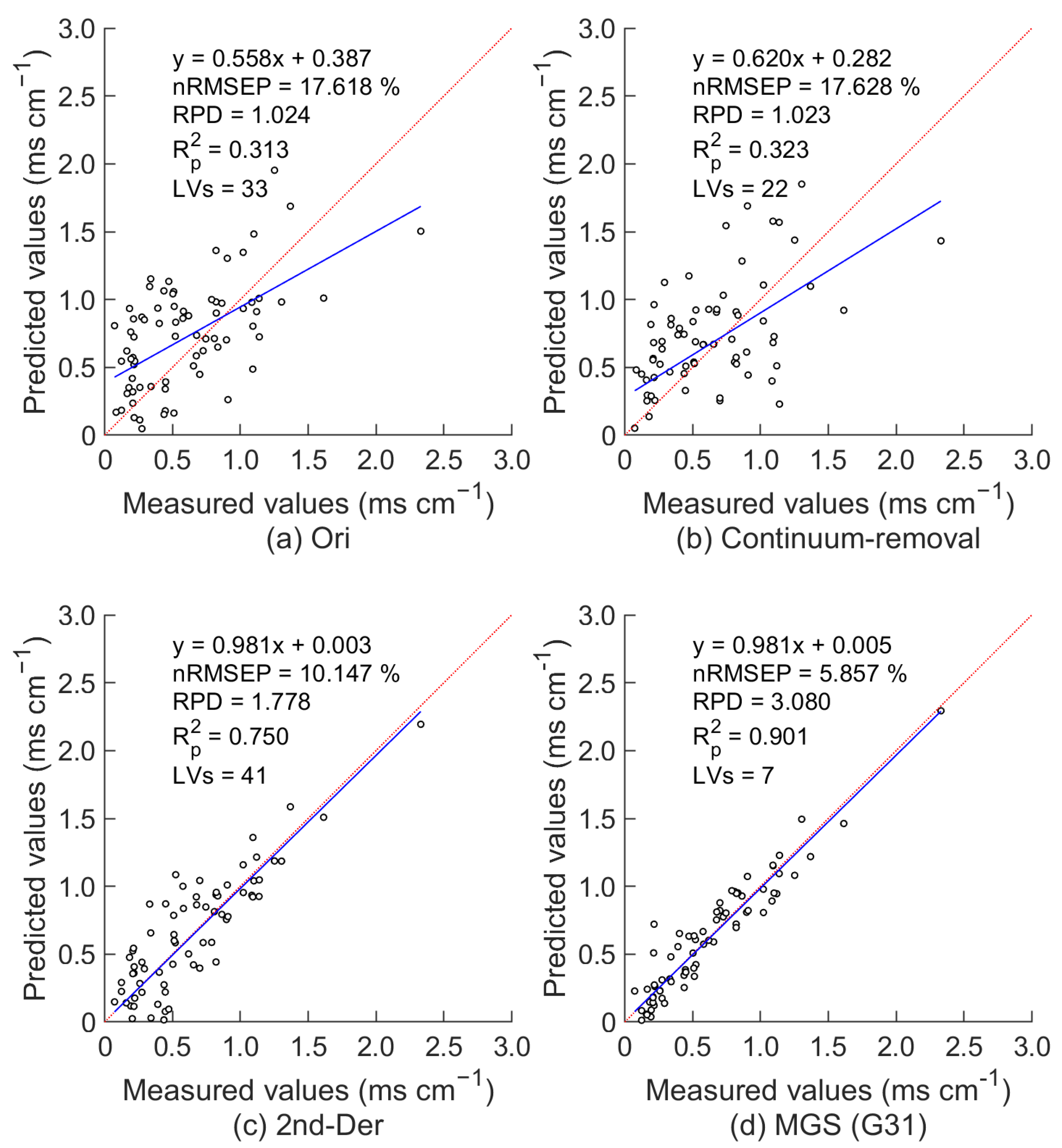
3.3. Model Accuracy Evaluation

The MGSS-PLSR model had the highest accuracy and stability, followed by 2nd-De-PLSR,1st-Der-PLSR, lnR-PLSR, 1/R-PLSR, CR-PLSR, Ori-PLSR, and R^0.5-PLSR models. When the granularity was 31, the estimation accuracy of the MGSS-PLSR model was the highest, with an R_c² of 0.95, R_p² of 0.90, RPD of 3.08, nRMSEC of 4.89%, and nRMSEP of 5.86%, and stability was also high. For the 2nd-Der-PLSR model, the R_c², nRMSEC, R_p², nRMSEP, and RPD were 0.94, 5.35%, 0.75, 10.15%, and 1.78, respectively. Moreover, there were great differences between nRMSEC and nRMSEP for the models constructed based on conventional spectral preprocessing methods, indicating the poor stability of the models (

Table 2. Evaluation of the accuracy of soil EC estimation models constructed using different spectral preprocessing methods.

Method	LVs	Rc2	nRMSEC (%)	Rp2	nRMSEP (%)	RPD
Ori	33	0.80	9.87	0.31	17.62	1.02
CR	22	0.77	10.73	0.32	17.63	1.02
1st-Der	28	0.94	5.61	0.65	10.94	1.65
2nd-De	41	0.94	5.35	0.75	10.15	1.78
1/R	30	0.77	10.73	0.33	17.49	1.03
R0.5	3	0.09	21.16	0.06	23.27	0.78
lnR	31	0.77	10.74	0.48	17.61	1.02
MGSS_31	7	0.95	4.89	0.90	5.86	3.08

Note: MGSS_31 represents the spectral features extracted at the granularity level of G31.

). Therefore, MGSS exhibited better performance than conventional spectral preprocessing methods.

3.4. Model Validation

Three optimal models (Ori, CR, and 2nd-Der) with an R_p² of 0.313, 0.323, and 0.750, respectively, and nRMSEP of 17.618%, 17.628%, and 10.147%, respectively, were selected. The fitting result between the estimates of the 2nd-Der-PLSR model and the measured values was better than that of Ori-PLSR and CR-PLSR models. However, the fitting result of the MGSS-PLSR model was optimal. In Figure 8, the points of the MGSS-PLSR model were close to the 1:1 line, indicating the high estimation accuracy of the model. The MGSS-PLSR model had the highest estimation accuracy among all models, with an R_p², RPD, and nRMSEP of 0.901, 3.080, and 5.857%, respectively. In addition, the R_p² and RPD of the MGSS-PLSR model increased by 0.151 and 1.302, respectively, and nRMSEP decreased by 4.29% compared with those of the 2nd-der-PLSR model, which is a model with the highest estimation accuracy that was constructed using conventional preprocessing methods. Therefore, MGSS can significantly improve soil EC estimation accuracy.

4. Discussion

4.1. Analysis of Spectral Features Extracted Based on Different Spectral Preprocessing Methods

Soil salinization is the gradual accumulation of soluble salts in the surface soil. Under the action of evaporation, deep soil water is transported to the surface through a soil capillary, which also brings the salt in the water to the surface (0–20 cm) [40]. The surface soil EC can effectively reflect the degree of soil salinization [1]. In recent years, with the development of precision agriculture, satellite- and unmanned-aerial-vehicle-based remote sensing have been widely used for large-scale soil salinity monitoring [41,42,43]. However, the spectra obtained are mixtures of soil and vegetation and cannot be directly used for soil EC estimation [44]. In addition, soil spectra are also affected by impurities, crop residues, and water content in field soil, making it difficult to extract the spectral features of soil EC [45,46]. Therefore, this study attempted to process soil EC spectra collected indoors using a variety of methods and to explore the feasibility and effectiveness of MGSS in extracting soil EC spectral features and estimation.

This study found that the correlation coefficient between MGSS preprocessed spectra and soil EC reached 0.3 (Figure 6), which was higher than that of conventional methods. Therefore, MGSS could significantly enhance the spectral information of soil EC and make the spectral features of soil EC become increasingly prominent with an increase in granularity level. It was also found that the spectral features extracted from 1st-Der and 2nd-Der preprocessed data were distributed uniformly. Therefore, 1st-Der and 2nd-Der could help extract the spectral information of soil parameters to a certain extent, which is similar to the results of Khosravi et al. [47] and Zhou et al. [48]. However, the spectral features extracted from other conventional method preprocessed data exhibited obvious aggregation (Figure 7), causing great difficulties for spectral feature extraction. It should be noted that the spectral features extracted from MGSS-preprocessed data had a wider distribution compared with those for conventional methods. Therefore, MGSS can highlight the spectral features of soil EC at different granularity levels, effectively excavate some hidden spectral information, and expand the spectral utilization range, thus improving model accuracy. The spectral features extracted from MGSS-G2 preprocessed data were mainly concentrated within 880–1200 nm, but the correlation analysis results (Figure 6b) showed that the spectral features should be around 700 nm. This may be because these spectral features at 700 nm are not extracted because of their excessively high redundancy. Wu et al. [49] found that the spectral features of soil EC were between 346 nm and 900 nm. This is different from our results. This may be due to differences in surface soil color, texture, structure, and surface roughness on the one hand and higher moisture content under vegetation cover and irrigation on the other hand [50]. In future studies, MGSS can be applied to field experiments in order to expand the universality of MGSS.

4.2. Comparison of the Estimation Accuracy of the Models Constructed Using Different Spectral Preprocessing Methods

Topography, climatic environment, soil physical and chemical properties, etc., affect the spectral reflectance of soil EC [51], so the construction of the soil EC estimation model is challenging. This study found that soil salinity had spatial heterogeneity. This is consistent with the study results of Guo et al. [52]. In recent years, scholars have developed methods for spectral feature extraction to improve soil salinity estimation accuracy. For example, Zhu et al. [53] and Farahmand and Sadeghi [54] improved soil salinity estimation accuracy by constructing normalized differential vegetation indices (NDVIs) and an S3 index ((G*R)/B). However, their methods have some defects. For example, the bands used in the construction of spectral indices are very close, resulting in the poor stability of the models [55]. Therefore, some scholars further improved soil salinity estimation accuracy by transforming raw spectra to extract more spectral features [56]. In this study, seven conventional methods and MGSS were used to preprocess spectral data for spectral feature extraction. Among the models constructed based on conventional methods, the accuracy of the 2nd-Der-PLSR model was the highest. However, it was still lower than that of the MGSS-PLSR model. The correlation to the soil EC of the spectra extracted after MGSS preprocessing was higher than that based on conventional methods, leading to the higher accuracy of the MGSS-PLSR model. It was found that at low granularity levels (G1–G3), the spectral features extracted were concentrated. With the increase in granularity level, the number of spectral features increased, and the distribution was discrete. Therefore, more spectral features could be extracted after MGSS preprocessing compared with conventional methods [57], especially with respect to weak spectral information. Kang and Zhang [20] and Pang et al. [58] also found that MGSS could significantly improve the accuracy and stability of forage protein content estimation and grassland biomass estimation. In short, more spectral features could be extracted after MGSS preprocessing, which could obviously improve the estimation accuracy. It should be noted that Pang et al. [58] reported that the combination of MGSS and the spectral index could obviously improve the accuracy of the estimation of grassland aboveground biomass (AGB) using satellite remote sensing. Therefore, the combination of the MGSS method and spectral index has the potential to improve the accuracy of the estimation model, and it can be applied to the inversion of soil parameters in the future.

Similarly to empirical mode decomposition [59], the essence of MGSS is the mathematical derivation of the raw spectrum. It can be regarded as an unsupervised decomposition of the spectrum, which can enhance the quantity and quality of spectral features extracted. However, in the continuous segmentation of the raw spectrum by MGSS, while extracting effective spectral information and weak spectral information, it also produces some independent spectral information that is not related to soil EC. In addition, with the increase in granularity level, the number of spectra produced increases exponentially, which may cause data redundancy. Therefore, research methods that use MGSS to extract effective spectral information while eliminating irrelevant spectral information and reducing data redundancy will be one of our future research priorities. In addition, soil EC has certain temporal and spatial variations due to environmental factors [60]. Therefore, some scholars extracted the spectral features of soil EC under the influences of vegetation cover using double extraction. That is, firstly, blind source separation (BSS) was used to extract soil reflectance from mixed spectra, and then soil parameter information was extracted from soil reflectance. After that, the soil parameter prediction model under vegetation cover was constructed. This method is mainly used for soil parameter estimation under vegetation cover with respect to satellite and UAV remote sensing [61], but estimating soil parameters under dense vegetation cover conditions is still difficult. In addition, methods for improving the accuracy of soil EC estimation in cotton fields and the matching accuracy of multi-scale (ground, UAV, and satellite remote sensing) spatiotemporal soil EC digital maps still need to be further explored. Therefore, we will apply MGSS to multi-scale spatiotemporal soil EC numerical modeling and mapping. On the one hand, this method can select a suitable growth environment for crops; on the other hand, it can monitor and evaluate the degree of soil salinization from multi-scale aspects so as to achieve accurate and efficient soil restoration and improve soil quality. It should be noted that Pang et al. [58] applied MGSS to preprocess Sentinel-2 images, and they found that MGSS could significantly improve the accuracy of the satellite estimation of grassland biomass. MGSS can reduce the loss of spectral information, extract weak spectral information, and enhance spectral features. Therefore, MGSS has the potential to improve the accuracy of the estimation of soil parameters using satellite data. This method also partially tackles the two difficult issues in satellite monitoring. Firstly, the number of spectral bands of multispectral satellites is limited, as the number is substantially lower than hyperspectral data, and some spectral features cannot be utilized. Secondly, although satellite sensors have a large monitoring range, they have a problem with low resolution compared to ground sensors, resulting in low accuracy and specificity in monitoring. MGSS can partially tackle the two difficult issues by extracting weak spectral information and reducing the loss of spectral information. This ultimately increases the accuracy of satellite monitoring.

5. Conclusions

In this study, the spectral reflectance and electrical conductivity of soils collected from cotton fields in southern Xinjiang, China, were determined indoors. Then, soil spectral data were preprocessed using MGSS and seven conventional methods. After that, a partial least squares regression (PLSR) model was constructed. Finally, the accuracies of the models were compared to determine the optimal soil EC estimation model. The results showed that the PLSR model constructed based on the second-order derivative (2nd-der-PLSR) had the highest estimation accuracy among the models constructed using conventional methods. However, among all models, the PLSR model constructed based on MGSS (MGSS-PLSR) had the highest estimation accuracy, with R_p² (0.901) and RPD (3.080) being 0.151 and 1.302 higher than those of the 2nd-der-PLSR model, respectively, and nRMSEP (5.857%) being 4.29% lower than that of the 2nd-der-PLSR model. The reason for the high accuracy of the MGSS-PLSR model is as follows: Compared with conventional spectral preprocessing methods, MGSS could greatly improve the correlation between spectra and soil EC, and it can disperse spectral features throughout the entire band. This can effectively extract the weak spectral information of soil EC in complex environments and expand the spectral utilization range. Thus, the quantity and quality of the extracted spectral features of soil EC are significantly improved by the MGSS, which further improves soil salinity estimation accuracy.

References

1. Wang, Z.; Zhang, F.; Zhang, X.; Chan, N.W.; Kung, H.; Ariken, M.; Zhou, X.; Wang, Y. Regional suitability prediction of soil salinization based on remote-sensing derivatives and optimal spectral index. Sci. Total Environ. 2021, 775, 145807. [Google Scholar] [CrossRef] [PubMed]
2. Sertel, E.; Gorji, T.; Tanik, A. Monitoring soil salinity via remote sensing technology under data scarce conditions: A case study from turkey. Ecol. Indic. 2017, 74, 384–391. [Google Scholar] [CrossRef]
3. Chen, H.; Zhao, G.; Li, Y.; Wang, D.; Ma, Y. Monitoring the seasonal dynamics of soil salinization in the Yellow River delta of China using Landsat data. Nat. Hazards Earth Syst. Sci. 2019, 19, 1499–1508. [Google Scholar] [CrossRef] [Green Version]
4. O’Neill, B.C.; Oppenheimer, M.; Warren, R.; Hallegatte, S.; Kopp, R.E.; Pörtner, H.O.; Scholes, R.; Birkmann, J.; Foden, W.; Licker, R.; et al. IPCC reasons for concern regarding climate changerisks. Nat. Clim. Chang. 2017, 7, 28–37. [Google Scholar] [CrossRef] [Green Version]
5. Zhang, J.Z.; Zou, R.; Wang, Z.H.; Zong, R.; Tan, M.D. Estimation of soil salt content in drip irrigation cotton field using GPR multi-frequency antenna amplitude envelope average method. J. Agric. Eng. 2021, 37, 99–107. [Google Scholar]
6. Llyas, N.R.M.M.T.; Shi, Q.G.; Abdulla, A.; Xia, N.; Wang, J.Z. Quantitative evaluation of soil salinization risk in Keriya Oasis based on grey evaluation model. J. Agric. Eng. 2019, 35, 176–184. [Google Scholar] [CrossRef]
7. Wang, J.; Ding, J.; Yu, D.; Teng, D.; He, B.; Chen, X.; Su, F. Machine learning-based detection of soil salinity in an arid desert region, Northwest China: A comparison between Landsat-8 OLI and Sentinel-2 MSI. Sci. Total Environ. 2020, 707, 136092. [Google Scholar] [CrossRef] [PubMed]
8. Wang, J.Z.; Ding, J.L.; Yu, D.L.; Ma, X.K.; Zhang, Z.P.; Ge, X.Y.; Teng, D.X.; Li, X.H.; Liang, J.; Lizaga, I.; et al. Capability of Sentinel-2 MSI data for monitoring and mapping of soil salinity in dry and wet seasons in the Ebinur Lake region, Xinjiang, China. Geoderma 2019, 353, 172–187. [Google Scholar] [CrossRef]
9. Sishodia, R.P.; Ray, R.L.; Singh, S.K. Applications of remote sensing in precision agriculture: A review. Remote Sens. 2020, 12, 3136. [Google Scholar] [CrossRef]
10. Fu, C.; Gan, S.; Yuan, X.; Xiong, H.; Tian, A. Determination of soil salt content using a probability neural network model based on particle swarm optimization in areas affected and non-affected by human activities. Remote Sens. 2018, 10, 1387. [Google Scholar] [CrossRef] [Green Version]
11. Shi, X.; Song, J.; Wang, H.; Lv, X. Monitoring soil salinization in Manas River Basin, Northwestern China based on multi-spectral index group. Eur. J. Remote Sens. 2021, 54 (Suppl. 2), 176–188. [Google Scholar] [CrossRef]
12. Wang, J.; Li, X. Comparison on quantitative inversion of characteristic ions in salinized soils with hyperspectral based on support vector regression and partial least squares regression. Eur. J. Remote Sens. 2020, 53, 340–348. [Google Scholar] [CrossRef]
13. Zhang, X.L.; Zhang, F.; Zhang, H.W.; Li, Z.; Hai, Q.; Chen, L.H. Optimization of soil salt inversion model based on spectral preprocessing from hyperspectral index. Trans. Chin. Soc. Agr. Eng. 2018, 34, 110–117. [Google Scholar]
14. Li, H.; Zhou, B.; Xu, F. Variation Analysis of Spectral Characteristics of Reclamation Vegetation in a Rare Earth Mining Area Under Environmental Stress. IEEE. Trans. Geosci. Remote Sens. 2022, 60, 4408412. [Google Scholar] [CrossRef]
15. Wang, J.Z.; Zhen, J.N.; Hu, W.F.; Chen, S.C.; Lizaga, I.; Zeraatpisheh, M.; Yang, X.D. Remote sensing of soil degradation: Progress and perspective. Int. Soil Water Conserv. 2023, 11, 429–454. [Google Scholar] [CrossRef]
16. Biney, J.K.M.; Blöcher, J.R.; Borůvka, L.; Vašát, R. Does the limited use of orthogonal signal correction pre-treatment approach to improve the prediction accuracy of soil organic carbon need attention? Geoderma 2021, 388, 114945. [Google Scholar] [CrossRef]
17. Zulfiqar, M.; Ahmad, M.; Sohaib, A.; Mazzara, M.; Distefano, S. Hyperspectral imaging for bloodstain identification. Sensors 2021, 21, 3045. [Google Scholar] [CrossRef] [PubMed]
18. Sun, Y.; Cai, W.; Shao, X. Chemometrics: An Excavator in Temperature-Dependent Near-Infrared Spectroscopy. Molecules 2022, 27, 452. [Google Scholar] [CrossRef]
19. Wang, J.Z.; Shi, T.Z.; Yu, D.L.; Teng, D.X.; Ge, X.Y.; Zhang, Z.P.; Yang, X.D.; Wang, H.X.; Wu, G.F. Ensemble machine-learning-based framework for estimating total nitrogen concentration in water using drone-borne hyperspectral imagery of emergent plants: A case study in an arid oasis, NW China. Environ. Pollut. 2020, 266, 115412. [Google Scholar] [CrossRef]
20. Kang, X.Y.; Zhang, W. Hyperspectral remote sensing estimation of pasture crude protein content based on multi-granularity spectral feature. J. Agric. Eng. 2019, 35, 161–169. [Google Scholar] [CrossRef]
21. Kang, X.Y.; Huang, C.P.; Zhang, L.F.; Zhang, Z.; Lv, X. Downscaling solar-induced chlorophyll fluorescence for field-scale cotton yield estimation by a two-step convolutional neural network. Comput. Electron. Agric. 2022, 201, 107260. [Google Scholar] [CrossRef]
22. Li, N. The Influence of American Sanctions on Cotton Growers in XPCC; Tarim University: Aral, China, 2022. [Google Scholar]
23. Tomaz, A.; Palma, P.; Alvarenga, P.; Gonçalves, M.C. Soil salinity risk in a climate change scenario and its effect on crop yield. Clim. Chang. Soil Interact. 2020, 351–396. [Google Scholar] [CrossRef]
24. Sidiropoulos, P.; Dalezios, N.R.; Loukas, A.; Mylopoulos, N.; Spiliotopoulos, M.; Faraslis, I.N.; Alpanakis, N.; Sakellariou, S. Quantitative classification of desertification severity for degraded aquifer based on remotely sensed drought assessment. Hydrology 2021, 8, 47. [Google Scholar] [CrossRef]
25. Helat, F.; Moncef, B.; Mourad, B.; Samir, B. Detection of terrain indices related to soil salinity and mapping sal-affected soils using remote sensing and geostatitical techniques. Environ. Monit. Assess. 2017, 189, 177–187. [Google Scholar] [CrossRef]
26. Zhang, J.H.; Jia, P.P.; Sun, Y.; Jia, K.L. Prediction of salinity ion content in different soil layers based on hyperspectral data. J. Agric. Eng. 2019, 35, 106–115. [Google Scholar] [CrossRef]
27. Xu, X.; Chen, Y.; Wang, M.; Wang, S.; Li, K.; Li, Y. Improving estimates of soil salt content by using two-date image spectral changes in Yinbei, China. Remote Sens. 2021, 13, 4165. [Google Scholar] [CrossRef]
28. Wang, X.P.; Jiang, F.C.; Wang, H.B.; Cao, H.; Yang, Y.P.; Gao, Y. Irrigation scheduling optimization of drip-irrigated without plastic film cotton in south Xinjiang based on Aqua Crop model. J. Agric. Mach. 2021, 52, 293–301. [Google Scholar]
29. Liu, J. The Applications of Remote Sensing Models of Soil Salinization Based on Feature Space; Xinjiang Agricultural University: Urumqi, China, 2022. [Google Scholar]
30. Luo, M.; Liu, T.; Meng, F.H.; Duan, Y.C.; Bao, B.M.; Xing, W.; Feng, X.W. Identifying climate change impacts on water resources in Xinjiang, China. Sci. Total Environ. 2019, 676, 613–626. [Google Scholar] [CrossRef]
31. Hu, J.; Peng, J.; Zhou, Y.; Xu, D.Y.; Zhao, R.Y.; Jiang, Q.S.; Fu, T.T.; Wang, F.; Shi, Z. Quantitative Estimation of SoilSalinity Using UAV-Borne Hyperspectral and Satellite Multispectral Images. Remote Sens. 2019, 11, 736. [Google Scholar] [CrossRef] [Green Version]
32. Benslama, A.; Khanchoul, K.; Benbrahim, F.; Boubehziz, S.; Chikhi, F.; Navarro-Pedreño, J. Monitoring the Variations of Soil Salinity in a Palm Grove in Southern Algeria. Sustainability 2020, 12, 6117. [Google Scholar] [CrossRef]
33. Kong, C.; Camps-Arbestain, M.; Clothier, B.; Bishop, P.; Vázquez, F.M. Reclamation of salt-affected soils using pumice and algal amendments: Impact on soil salinity and the growth of lucerne. Environ. Technol. Innov. 2021, 24, 101867. [Google Scholar] [CrossRef]
34. Ren, J.H.; Chen, Q.; Ma, D.L.; Xie, R.F.; Zhu, H.L.; Zang, S.Y. Study on a fast EC measurement method of soda saline-alkali soil based on wavelet decomposition texture feature. Catena 2021, 203, 105272. [Google Scholar] [CrossRef]
35. Kang, X.Y.; Zhang, W. A novel method for high-order residual quantization-based spectral binary coding. Spectrosc. Spect. Anal. 2019, 39, 3013–3020. [Google Scholar]
36. Mendoza, F.A.; Wiesinger, J.A.; Lu, R.; Nchimbi-Msolla, S.; Miklas, P.N.; Kelly, J.D.; Cichy, K.A. Prediction of cooking time for soaked and unsoaked dry beans (Phaseolus vulgaris L.) using hyperspectral imaging technology. Plant. Phenome J. 2018, 1, 1–9. [Google Scholar] [CrossRef] [Green Version]
37. Pan, B.; Yu, H.; Cheng, H.; Du, S.; Feng, S.; Shu, Y.; Du, J.; Xie, H. Machine Learning Model of Hydrothermal Vein Copper Deposits at Meso-Low Temperatures Based on Visible-Near Infrared Parallel Polarized Reflectance Spectroscopy. Minerals 2022, 12, 1451. [Google Scholar] [CrossRef]
38. Chen, W.H.; Chen, H.Z.; Feng, Q.X.; Mo, L.N.; Hong, S.Y. A hybrid optimization method for sample partitioning in near-infrared analysis. Spectrochim. Acta A 2021, 248, 119182. [Google Scholar] [CrossRef]
39. Zhao, Y.; Zhao, Z.; Shan, P.; Peng, L.S.; Yu, J.L.; Gao, D.L. Calibration transfer based on affine invariance for NIR without transfer standards. Molecules 2019, 24, 1802. [Google Scholar] [CrossRef] [Green Version]
40. Solangi, K.A.; Siyal, A.A.; Wu, Y.; Abbasi, B.; Solangi, F.; Lakhiar, I.A.; Zhou, G. An Assessment of the Spatial and Temporal Distribution of Soil Salinity in Combination with Field and Satellite Data: A Case Study in Sujawal District. Agronomy 2019, 9, 869. [Google Scholar] [CrossRef] [Green Version]
41. Ivushkin, K.; Bartholomeus, H.; Bregt, A.K.; Pulatov, A.; Franceschini, M.H.D.; Kramer, H.; van Loo, E.N.; Jaramillo Roman, V.; Finkers, R. UAV based soil salinity assessment of cropland. Geoderma 2019, 338, 502–512. [Google Scholar] [CrossRef]
42. Zhang, S.; Zhao, G. A Harmonious Satellite-Unmanned Aerial Vehicle-Ground Measurement Inversion Method for Monitoring Salinity in Coastal Saline Soil. Remote Sens. 2019, 11, 1700. [Google Scholar] [CrossRef] [Green Version]
43. Qi, G.; Chang, C.; Yang, W.; Gao, P.; Zhao, G. Soil Salinity Inversion in Coastal Corn Planting Areas by the Satellite-UAV-Ground Integration Approach. Remote Sens. 2021, 13, 3100. [Google Scholar] [CrossRef]
44. Liu, Y.; Zhang, F.; Wang, C.; Wu, S.; Liu, J.; Xu, A.; Pan, K.; Pan, X. Estimating the soil salinity over partially vegetated surfaces from multispectral remote sensing image using non-negative matrix factorization. Geoderma 2019, 354, 113887. [Google Scholar] [CrossRef]
45. Sankey, J.B.; Sankey, T.T.; Li, J.; Ravi, S.; Wang, G.; Caster, J.; Kasprak, A. Quantifying plant-soil-nutrient dynamics in rangelands: Fusion of UAV hyperspectral-LiDAR, UAV multispectral-photogrammetry, and ground-based LiDAR-digital photography in a shrub-encroached desert grassland. Remote Sens. Environ. 2021, 253, 112223. [Google Scholar] [CrossRef]
46. Wang, J.Z.; Hu, X.J.; Shi, T.Z.; He, L.; Hu, W.F.; Wu, G.F. Assessing toxic metal chromium in the soil in coal mining areas via proximal sensing: Prerequisites for land rehabilitation and sustainable development. Geoderma 2022, 405, 115399. [Google Scholar] [CrossRef]
47. Khosravi, V.; Doulati Ardejani, F.; Yousefi, S.; Aryafar, A. Monitoring soil lead and zinc contents via combination of spectroscopy with extreme learning machine and other data mining methods. Geoderma 2018, 318, 29–41. [Google Scholar] [CrossRef]
48. Zhou, W.; Yang, H.; Xie, L.; Li, H.; Huang, L.; Zhao, Y.; Yue, T. Hyperspectral inversion of soil heavy metals in Three-River Source Region based on random forest model. Catena 2021, 202, 105222. [Google Scholar] [CrossRef]
49. Wu, D.; Jia, K.; Zhang, X.; Zhang, J.; Abd El-Hamid, H.T. Remote Sensing Inversion for Simulation of Soil Salinization Based on Hyperspectral Data and Ground Analysis in Yinchuan, China. Nat. Resour. Res. 2021, 30, 4641–4656. [Google Scholar] [CrossRef]
50. Mandal, A.K. The need for the spectral characterization of dominant salts and recommended methods of soil sampling and analysis for the proper spectral evaluation of salt affected soils using hyper-spectral remote sensing. Remote Sens. Lett. 2022, 13, 588–598. [Google Scholar] [CrossRef]
51. Wang, X.; Song, K.; Wang, Z.; Li, S.; Zheng, M.; Wen, Z.; Liu, G. Are topsoil spectra or soil-environmental factors better indicators for discrimination of soil classes? Catena 2022, 218, 106580. [Google Scholar] [CrossRef]
52. Guo, B.; Zang, W.; Luo, W.; Wen, Y.; Yang, F.; Han, B.; Yang, X. Detection model of soil salinization information in the Yellow River Delta based on feature space models with typical surface parameters derived from Landsat8 OLI image. Geomat. Nat. Hazards Risk 2020, 11, 288–300. [Google Scholar] [CrossRef]
53. Zhu, K.; Sun, Z.; Zhao, F.; Yang, T.; Tian, Z.; Lai, J.; Long, B. Relating hyperspectral vegetation indices with soil salinity at different depths for the diagnosis of winter wheat salt stress. Remote Sens. 2021, 13, 250. [Google Scholar] [CrossRef]
54. Farahmand, N.; Sadeghi, V. Estimating Soil Salinity in the dried lake bed of urmia lake using pptical sentinel-2 images and nonlinear regression models. J. Indian Soc. Remote 2020, 48, 675–687. [Google Scholar] [CrossRef]
55. Zhou, X.X.; Li, Y.Y.; Luo, Y.K.; Sun, Y.W.; Su, Y.J.; Tan, C.W.; Liu, Y.J. Research on remote sensing classification of fruit trees based on Sentinel-2 multi-temporal imageries. Sci. Rep. 2022, 12, 11549. [Google Scholar] [CrossRef] [PubMed]
56. Duan, P.C.; Xiong, H.G.; Li, R.R.; Zhang, L. A quantitative analysis of the reflectance of the saline soil under different disturbance extent. Spectrosc. Spect. Anal. 2017, 37, 571–576. [Google Scholar]
57. Yasenjiang, K.; Yang, S.T.; Negra, T.S.F.T.; Zhang, F. Hyperspectral estimation of soil electrical conductivity based on fractional order differentially optimised spectral indices. J. Ecol. 2019, 39, 7237–7248. [Google Scholar] [CrossRef]
58. Pang, H.Y.; Zhang, A.W.; Kang, X.Y.; He, N.P.; Dong, G. Estimation of the grassland aboveground biomass of the inner mongolia plateau using the simulated spectra of sentinel-2 Images. Remote Sens. 2020, 12, 4155. [Google Scholar] [CrossRef]
59. Özger, M.; Başakın, E.E.; Ekmekcioğlu, Ö.; Hacısüleyman, V. Comparison of wavelet and empirical mode decomposition hybrid models in drought prediction. Comput. Electron. Agric. 2020, 179, 105851. [Google Scholar] [CrossRef]
60. Fathizad, H.; Ardakani, M.A.H.; Sodaiezadeh, H.; Kerry, R.; Taghizadeh-Mehrjardi, R. Investigation of the spatial and temporal variation of soil salinity using random forests in the central desert of Iran. Geoderma 2020, 365, 114233. [Google Scholar] [CrossRef]
61. Ouerghemmi, W.; Gomez, C.; Naceur, S.; Lagacherie, P. Semi-blind source separation for the estimation of the clay content over semi-vegetated areas using VNIR/SWIR hyperspectral airborne data. Remote Sens. Environ. 2016, 181, 251–263. [Google Scholar] [CrossRef]
Figure 1. Distribution of cotton fields for soil sampling in southern Xinjiang, China.
Remotesensing 15 03358 g001
Figure 2. Selection of sampling points.
Remotesensing 15 03358 g002
Figure 3. Soil spectral data acquisition.
Remotesensing 15 03358 g003
Figure 4. Spectral feature extraction by multi-granularity spectral segmentation (MGSS). (a) is the raw spectrum, and (br) denotes the segmentation lines, approximate spectra, and spectral features at granularity 1–6, respectively.
Remotesensing 15 03358 g004
Figure 5. Flow chart of modeling.
Remotesensing 15 03358 g005
Figure 6. Correlation between spectral reflectance and soil EC based on conventional spectral preprocessing methods (a) and MGSS (b).
Remotesensing 15 03358 g006
Figure 7. Distribution of spectral features after spectral preprocessing using conventional methods (a) and MGSS (b).
Remotesensing 15 03358 g007
Figure 8. Validation of soil EC estimation models constructed using different spectral preprocessing methods.
Remotesensing 15 03358 g008