


Enhanced Absence Sampling Technique for Data-Driven Landslide Susceptibility Mapping: A Case Study in Songyang County, China


Abstract
1. Introduction
2. Materials
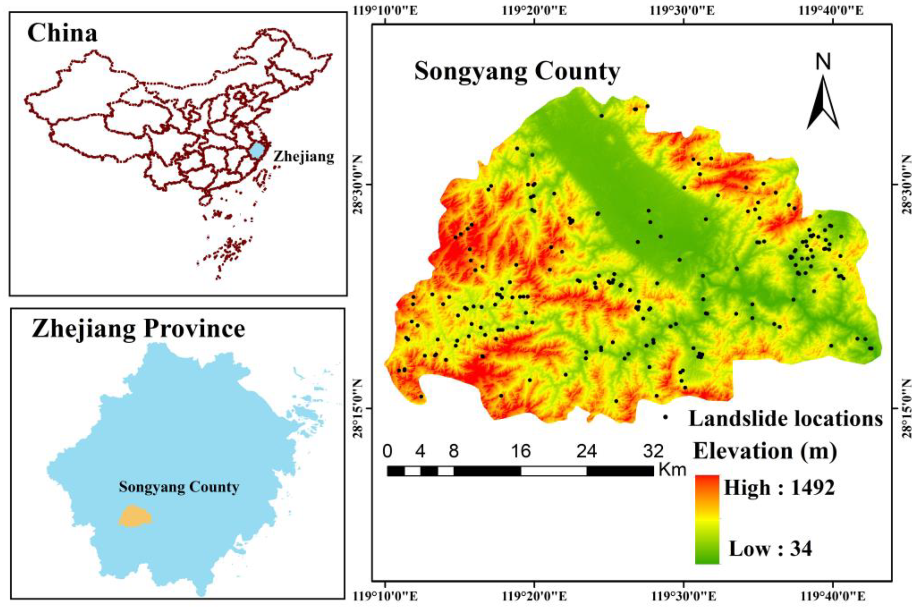
2.1. Study Area
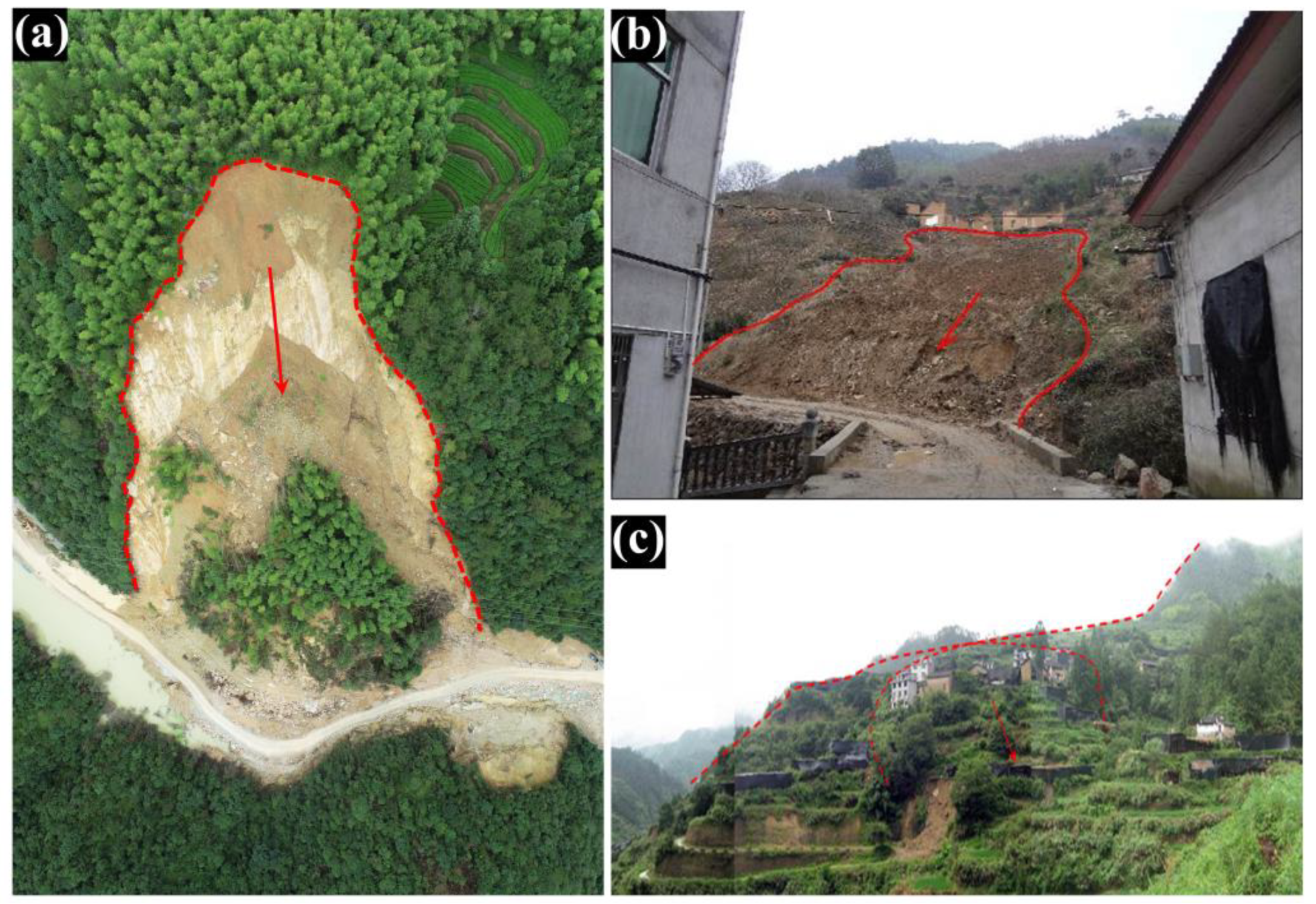
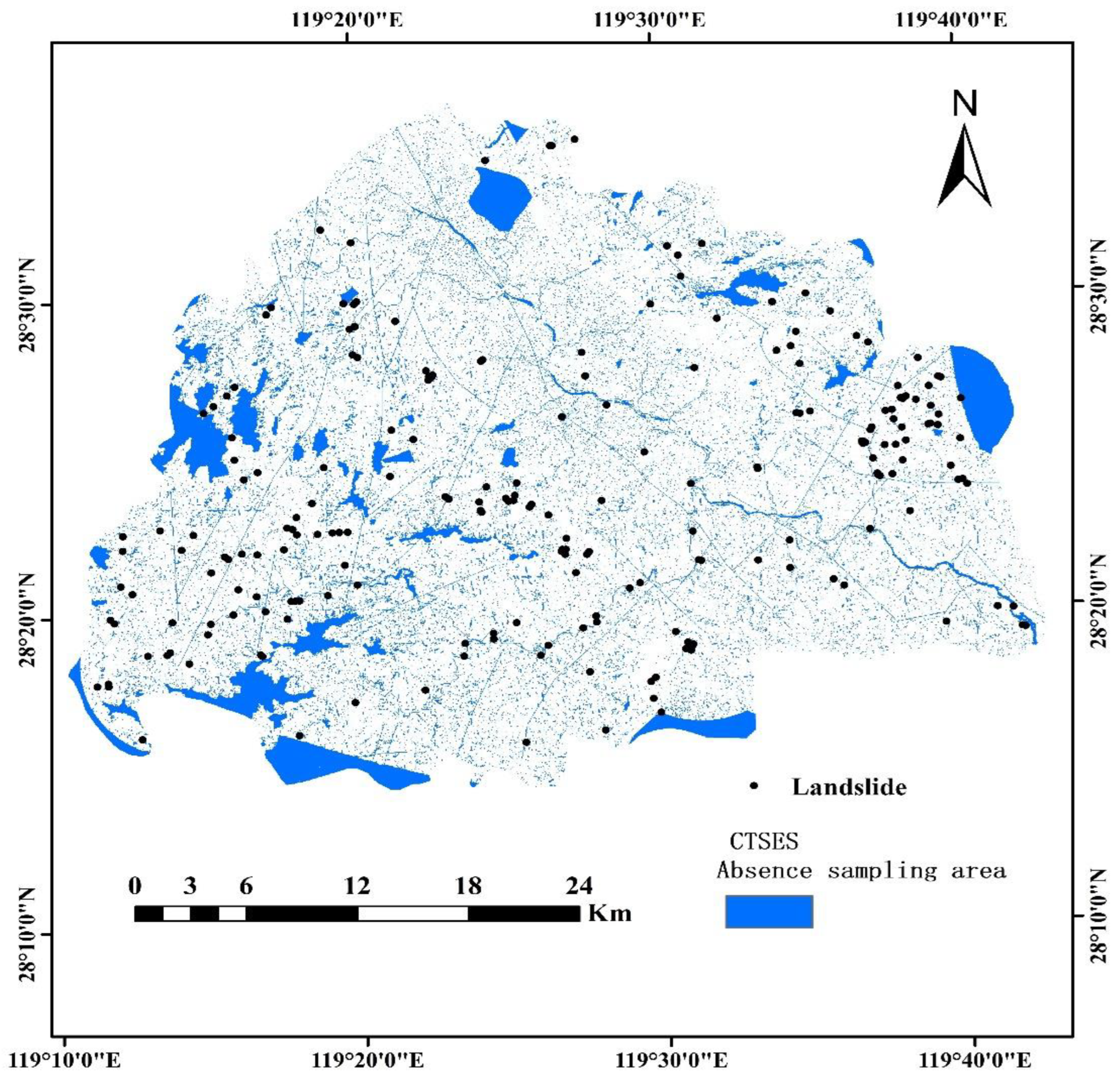
2.2. Landslide Inventory
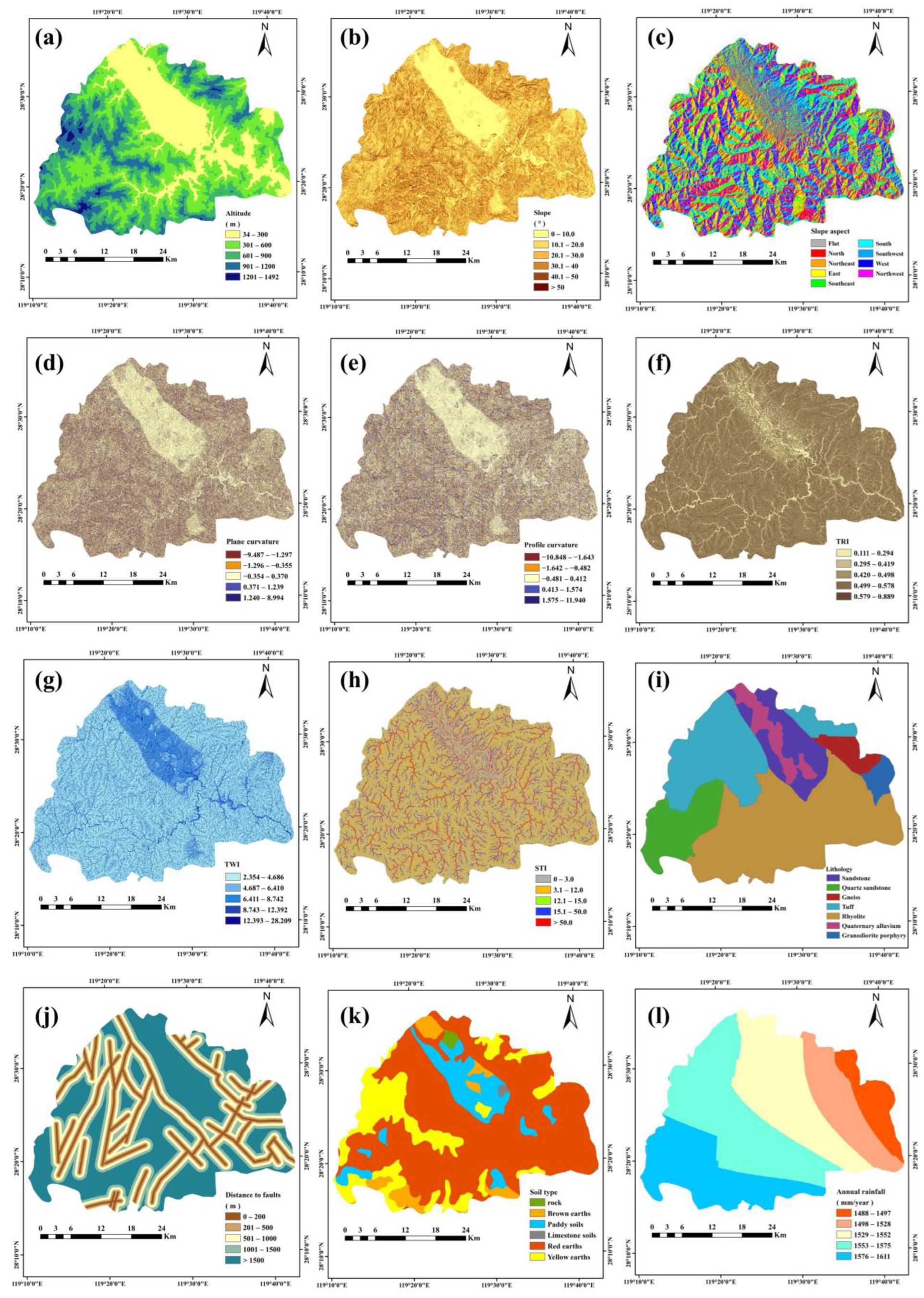
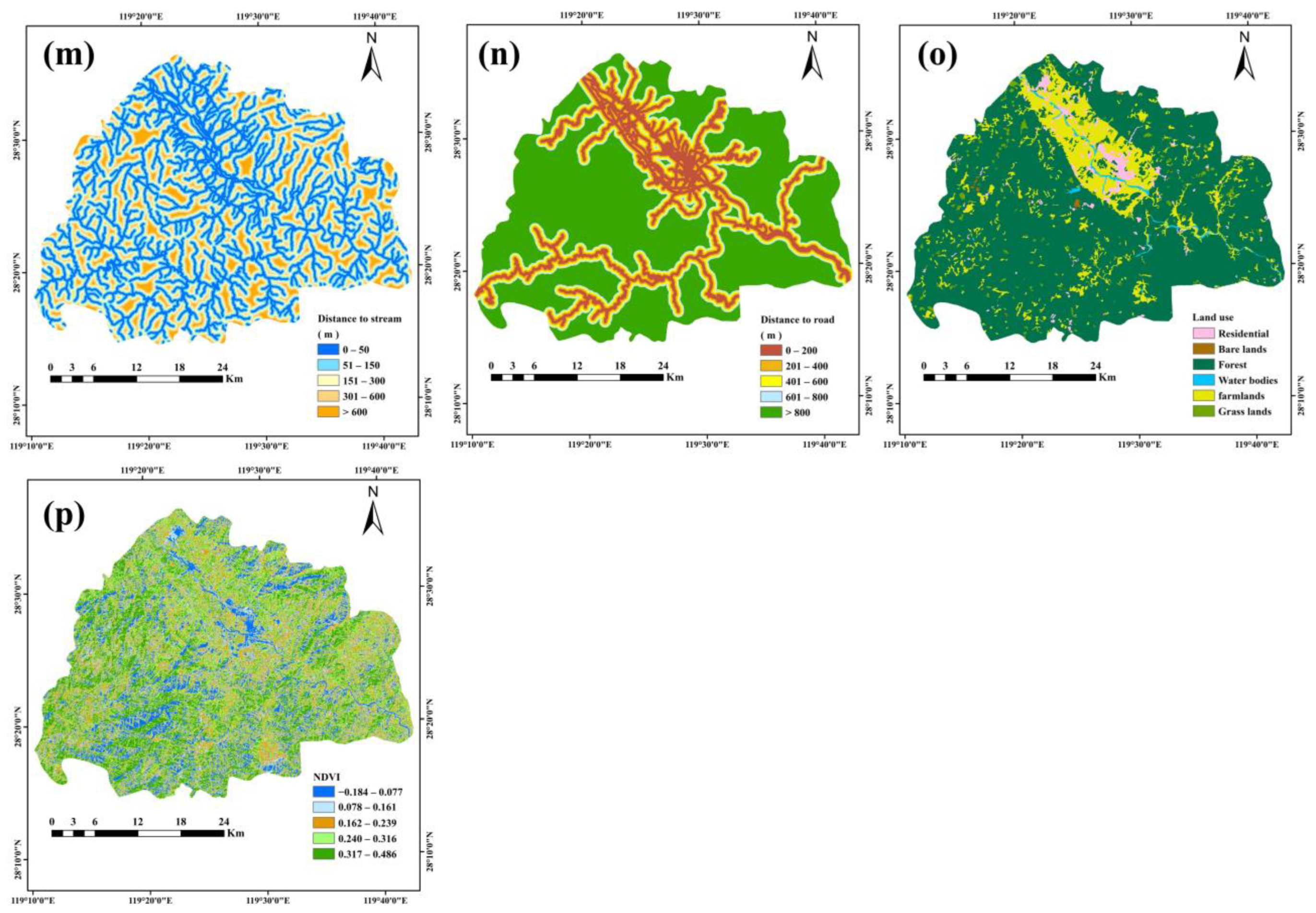
2.3. Landslide Conditioning Factors
3. Methodology
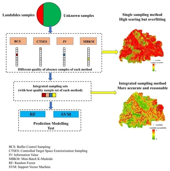
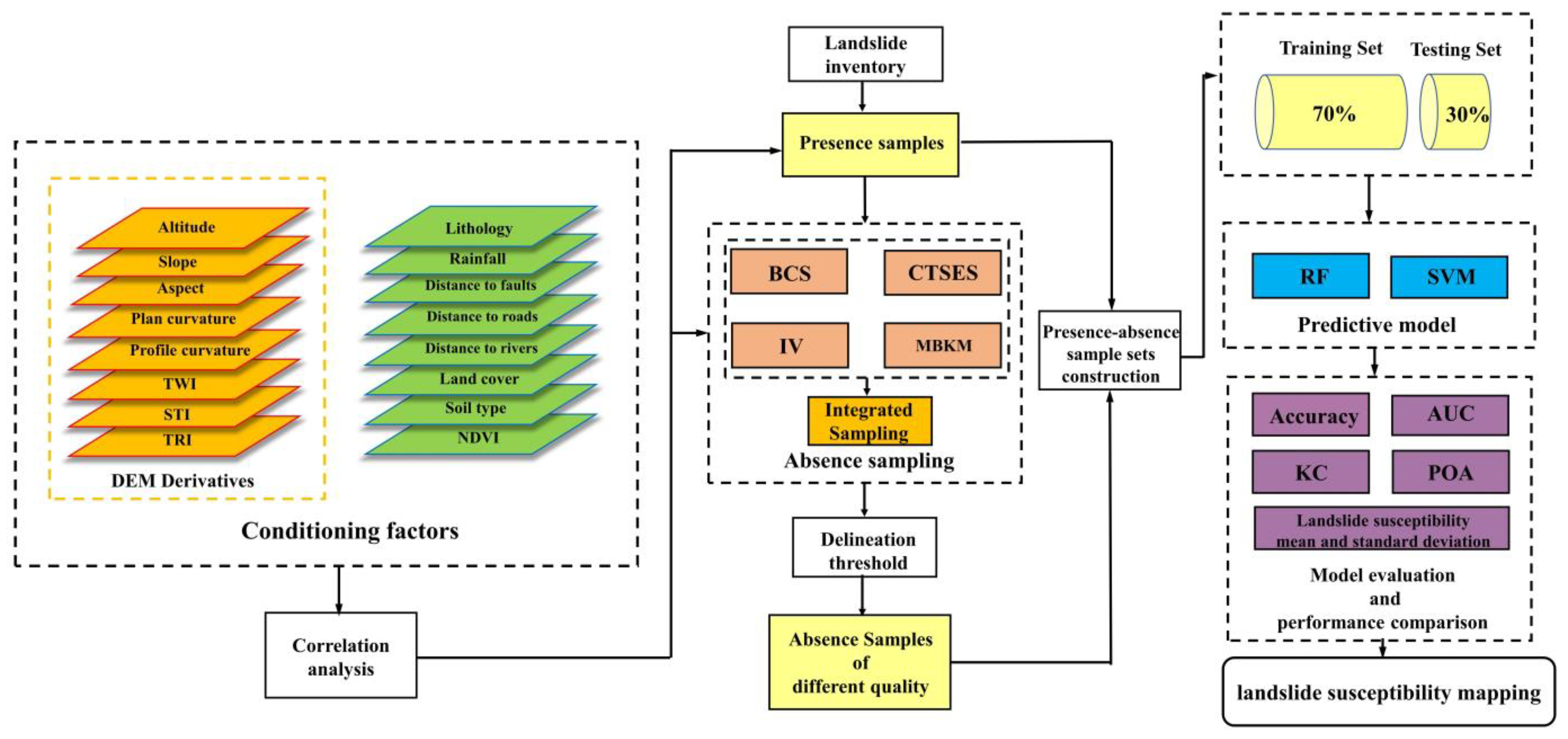
3.1. Study Route
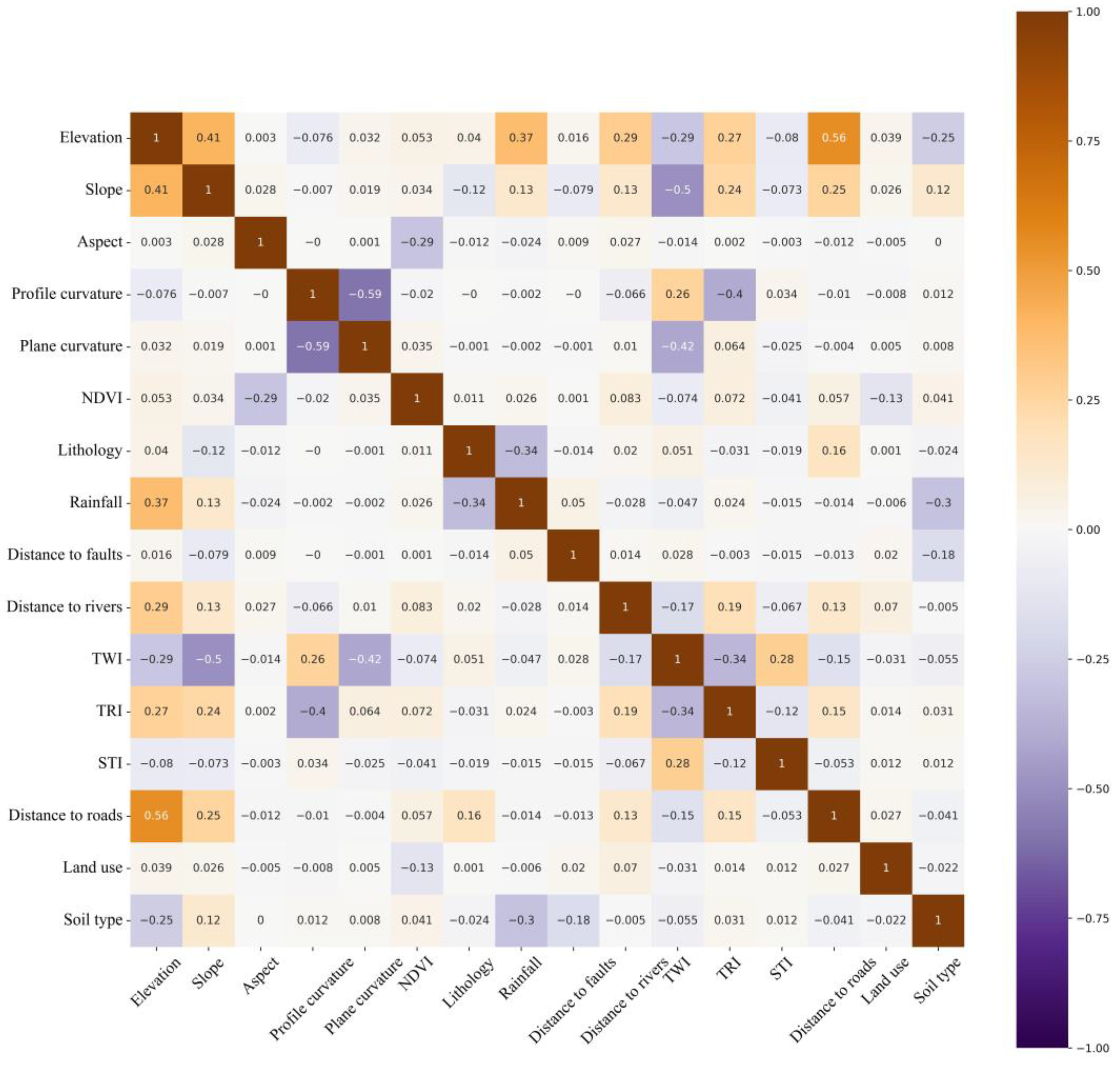
3.2. Correlation Analysis of Conditioning Factors
3.3. Absence Sampling Methods
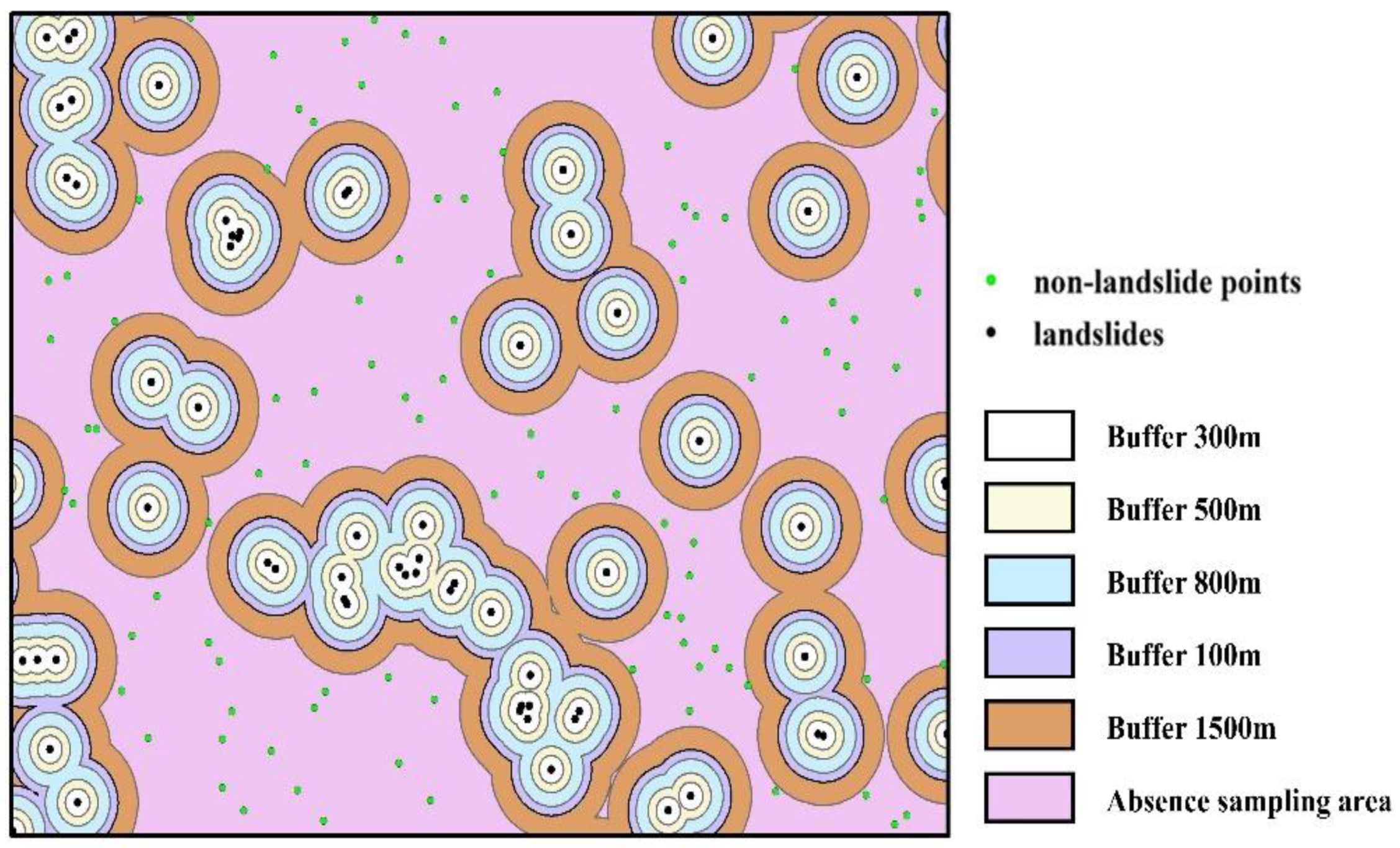
3.3.1. Buffer Control Sampling (BCS)
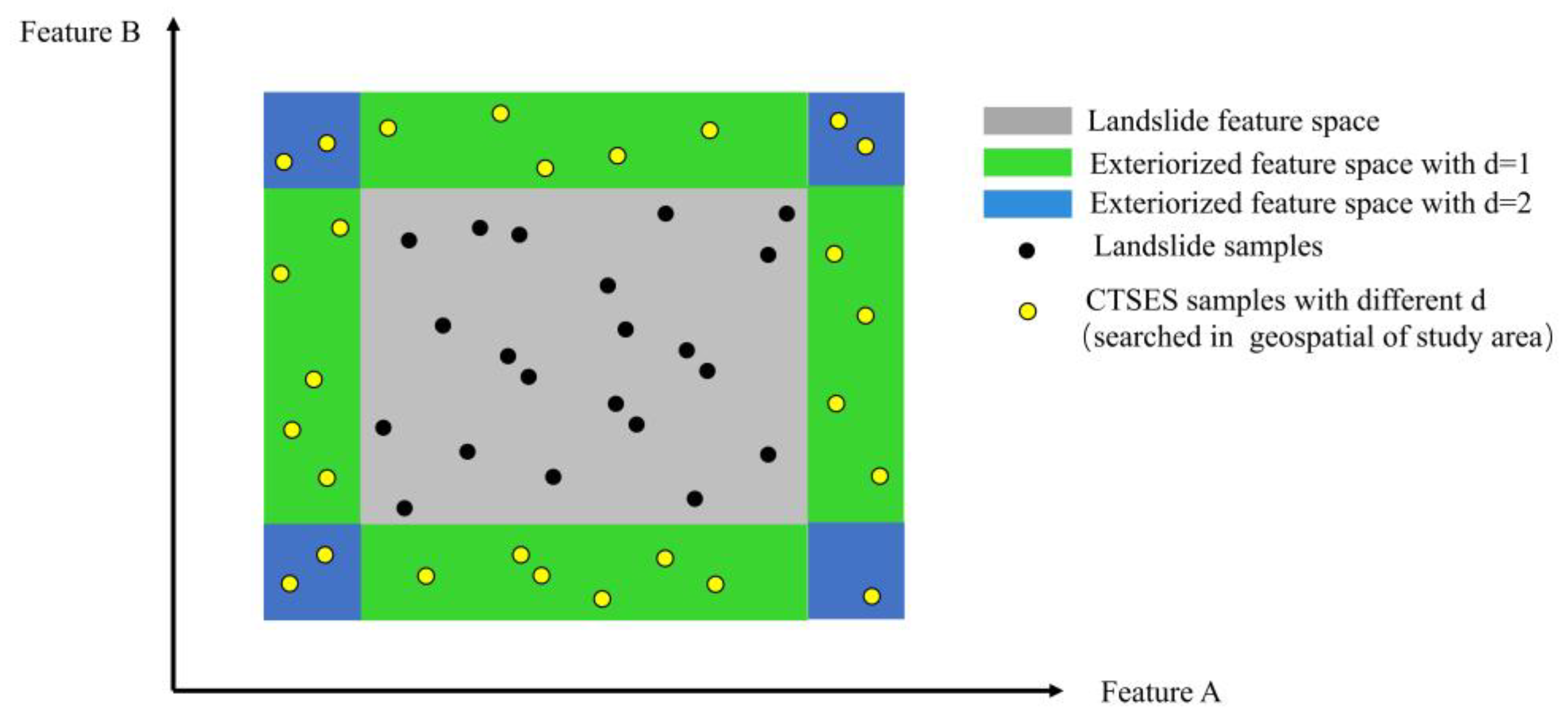
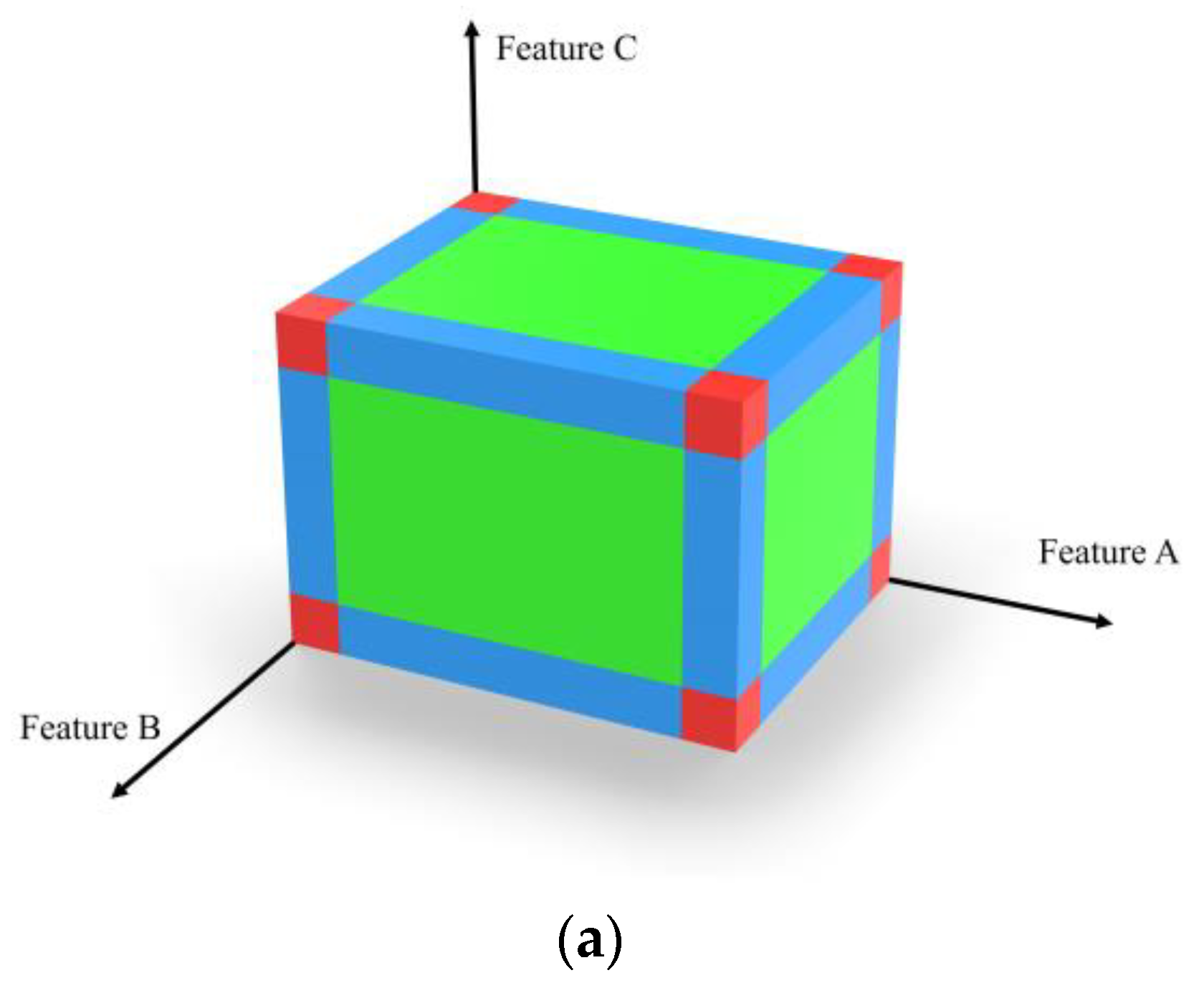
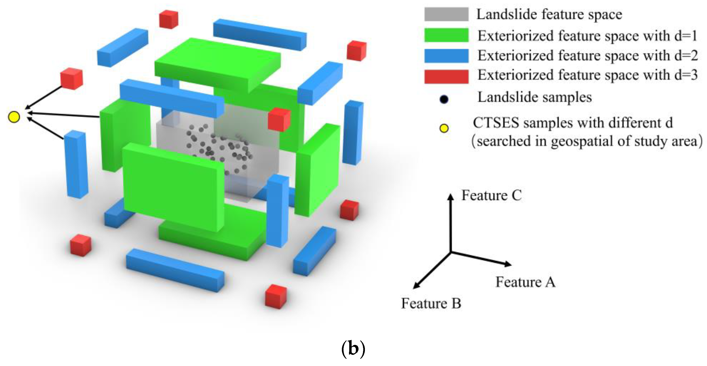
3.3.2. Controlled Target Space Exteriorization Sampling (CTSES)
- (1)
- Initialization:
- (2)
- For each landslide conditioning factor A:
- (3)
- Traverse every unit i in the study area:
- (a)
- Set temporary variables a = 0;
- (b)
- Traverse every landslide conditioning factor A:if A of i is in , a = a + 1;
- (c)
- If a = d, then run (d):
- (d)
- Nd = Nd ∪ i
- (4)
- Return Nd
3.3.3. Information Value (IV)
3.3.4. Mini-Batch K-Medoids (MBKM)
- K initial centroids are randomly selected.
- Assign the remaining points to the cluster represented by the closest medoids.
- In each class, the sum of distances between each sample point and other points is calculated, and the point with the smallest sum of distances is selected as the new medoid.
- Repeat the process in steps 2–3 until all medoid points no longer change or the upper limit of iterations is reached.
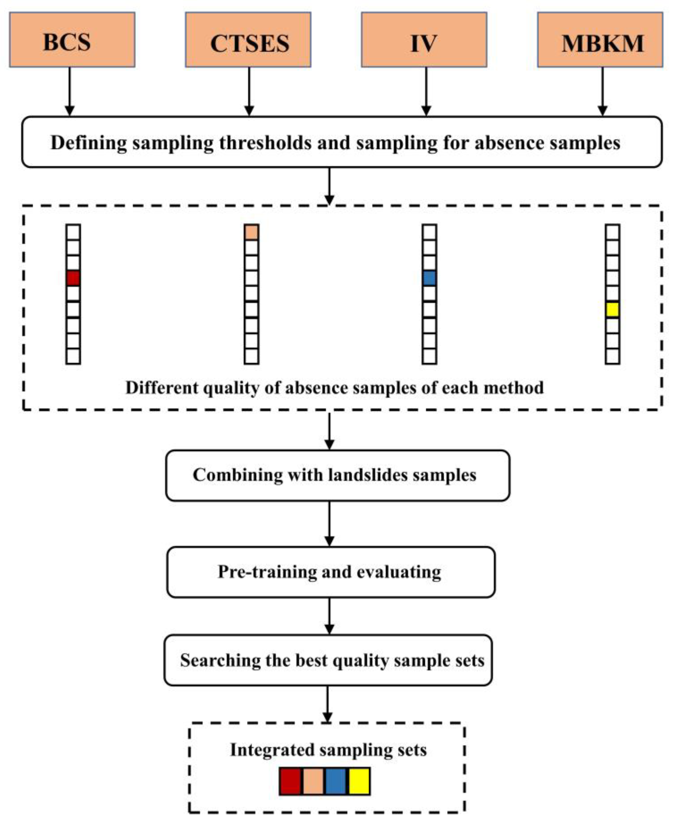
3.3.5. Integrative Sampling
3.4. Machine Learning for Landslide Susceptibility Mapping
3.4.1. Random Forest
3.4.2. Support Vector Machine
3.5. Model Evaluation Methods
4. Results
4.1. Correlation Analysis
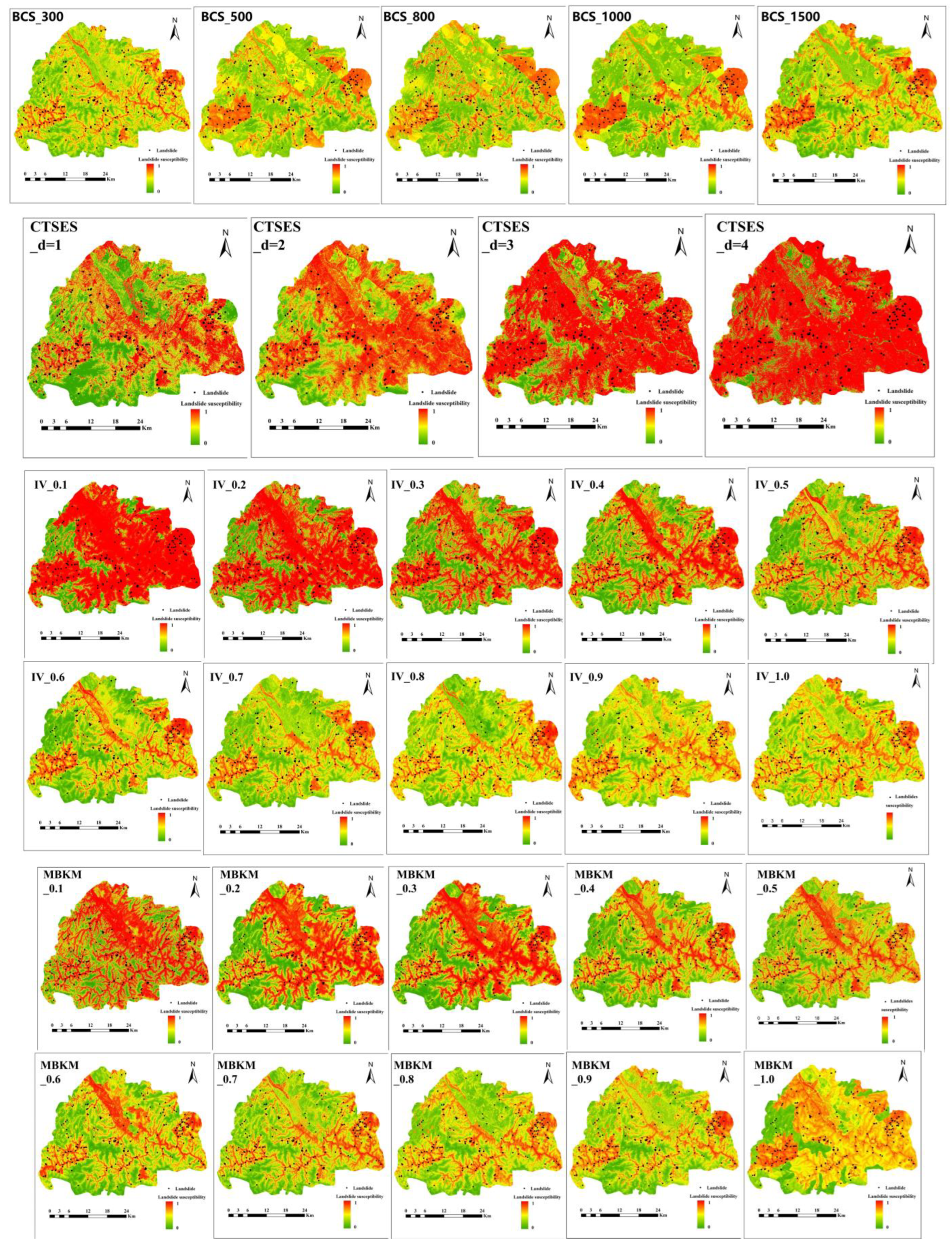
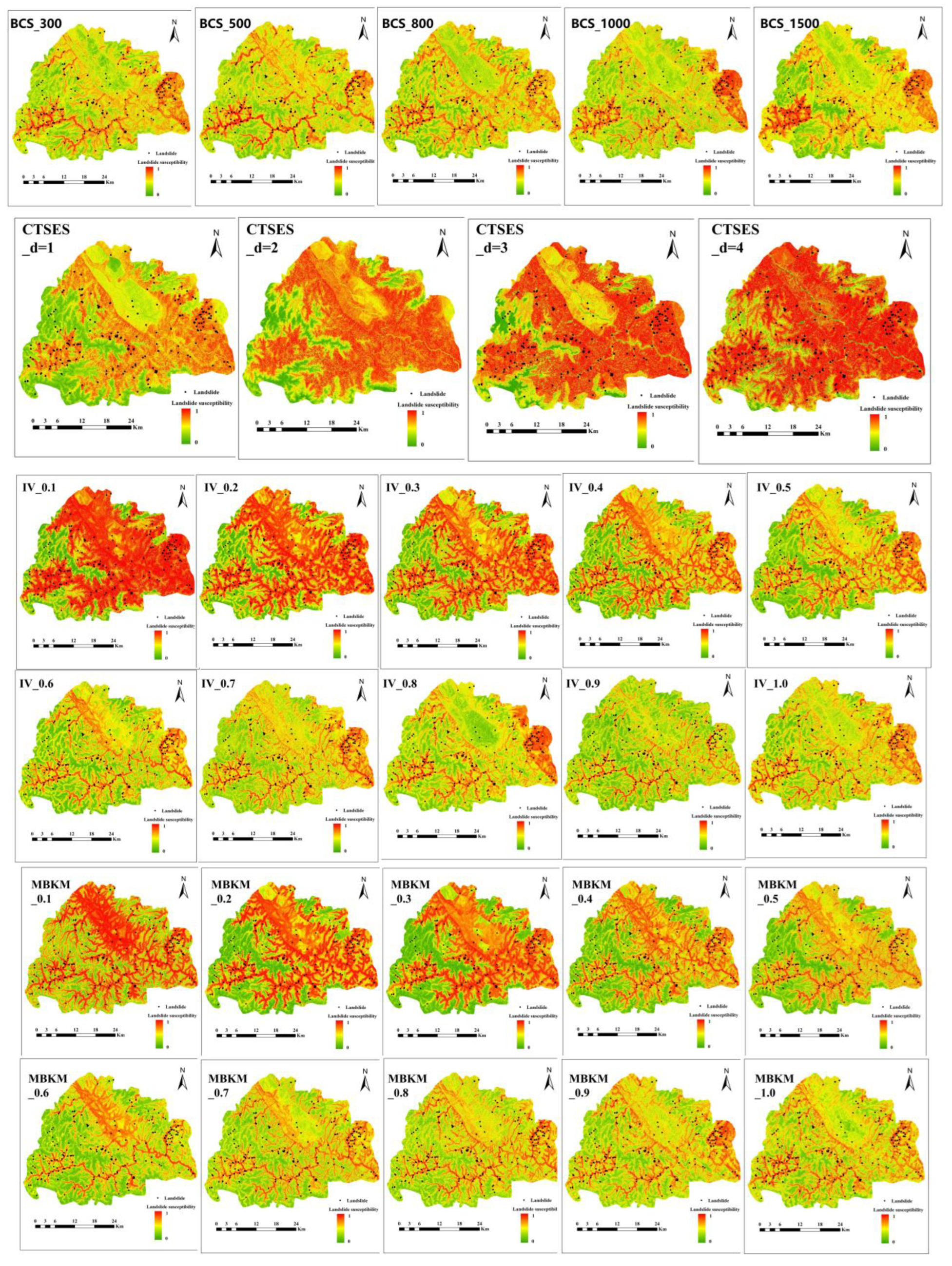
4.2. Results of Absence Sampling
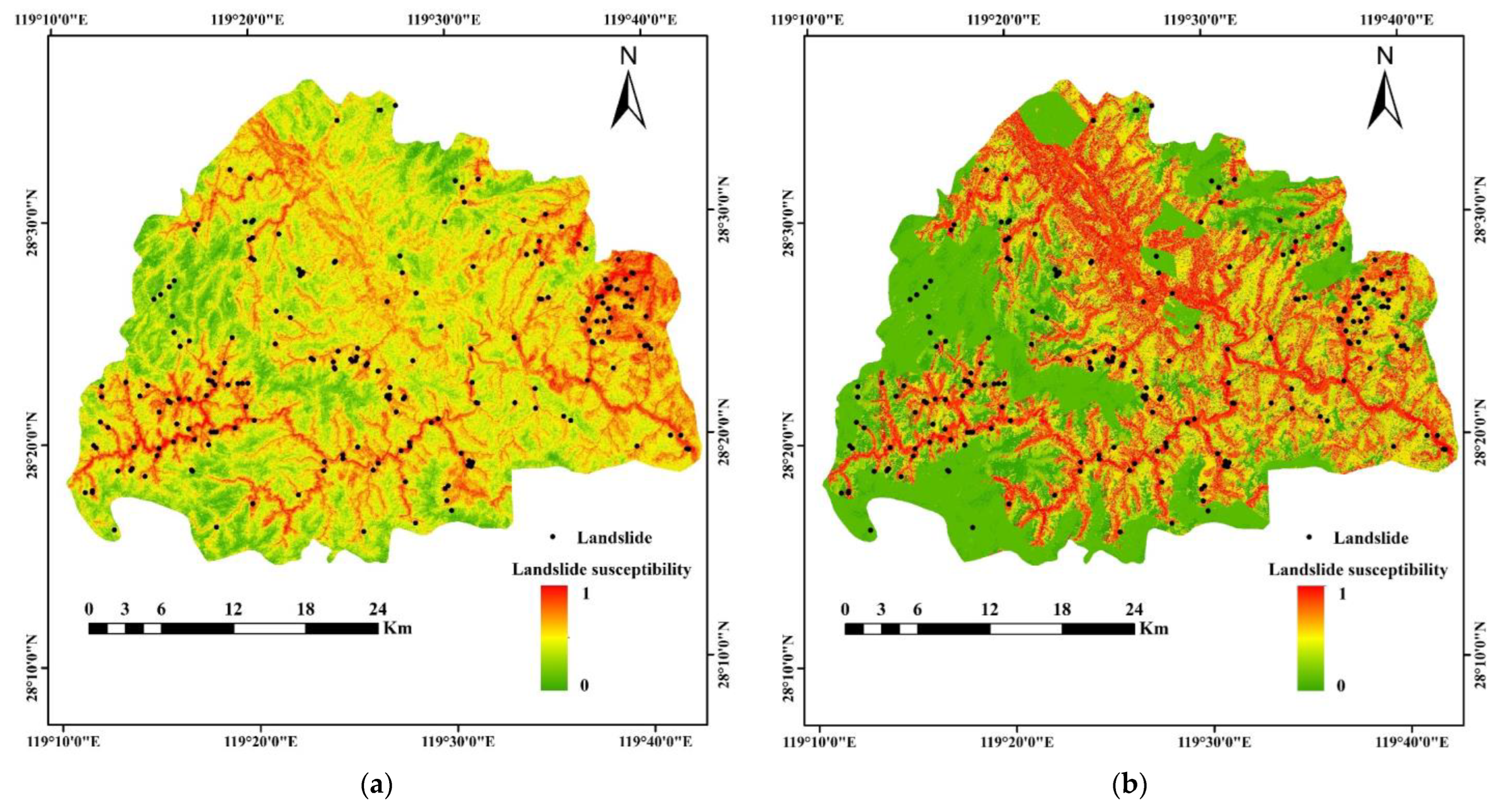
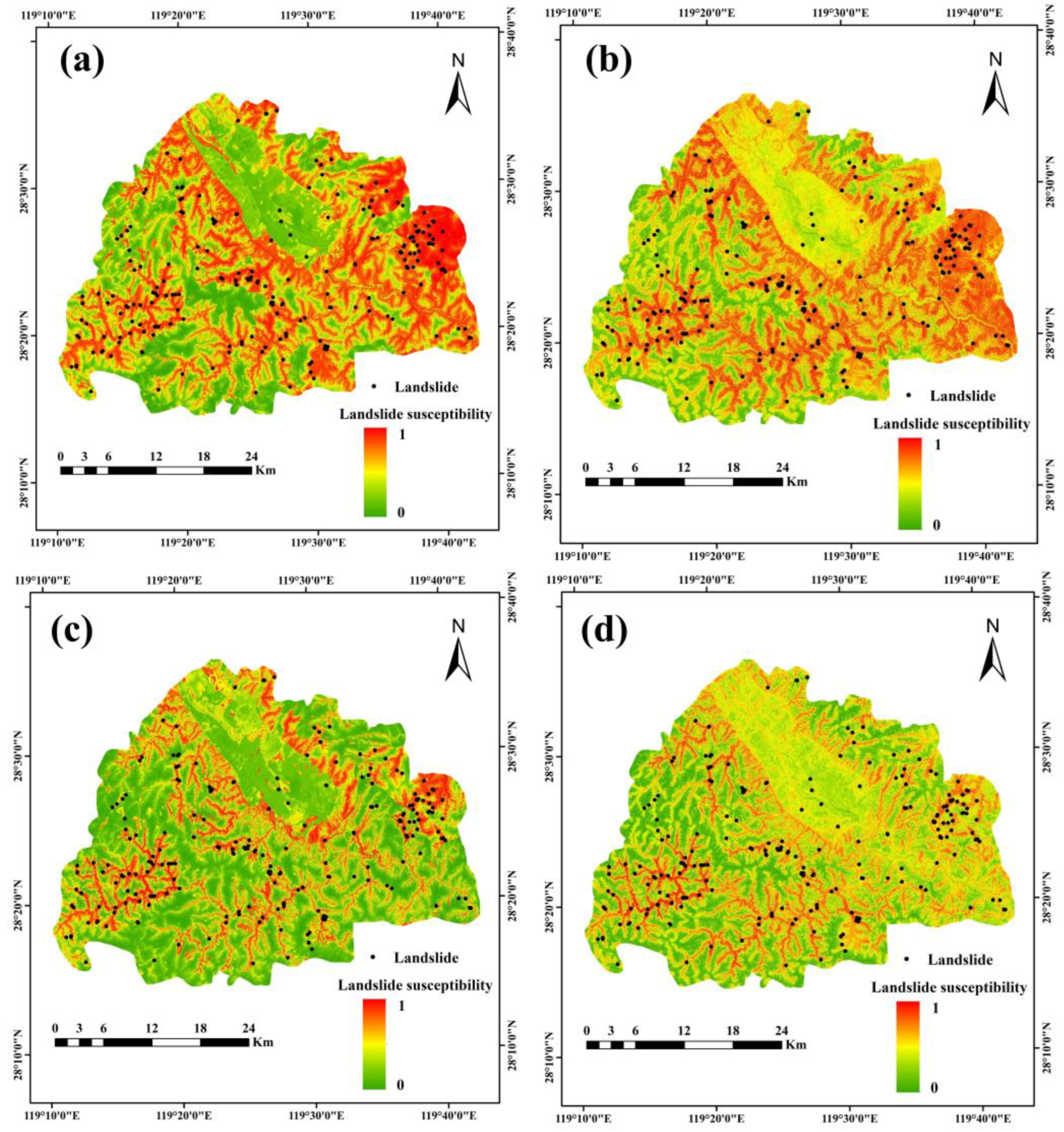
4.3. Landslide Susceptibility Mapping
4.3.1. LSM Results for Four Sampling Strategies with Different Sampling Intervals
4.3.2. LSM Results of the Integrative Sampling Method
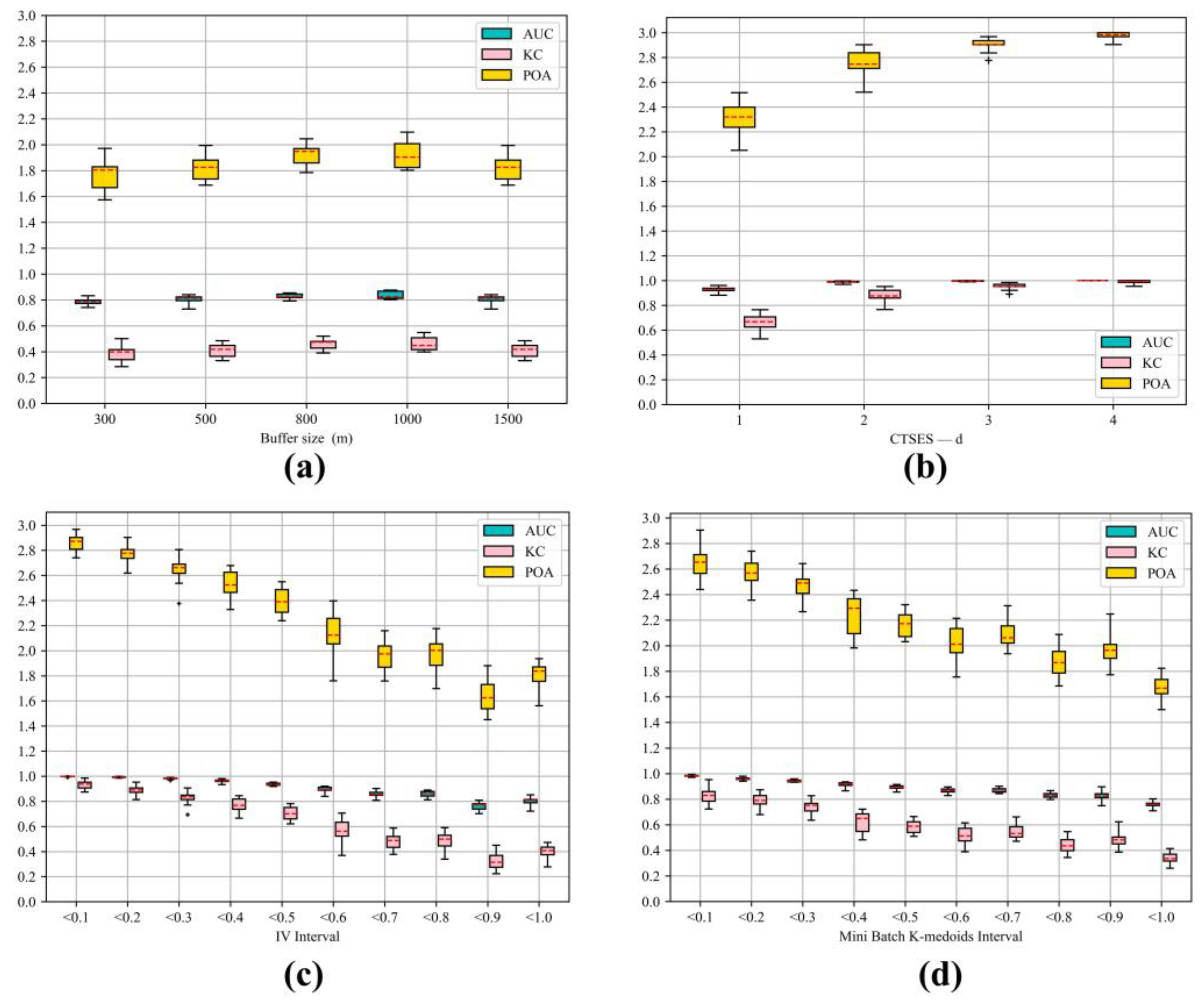
4.4. Evaluation of Different Absence Sampling Methods
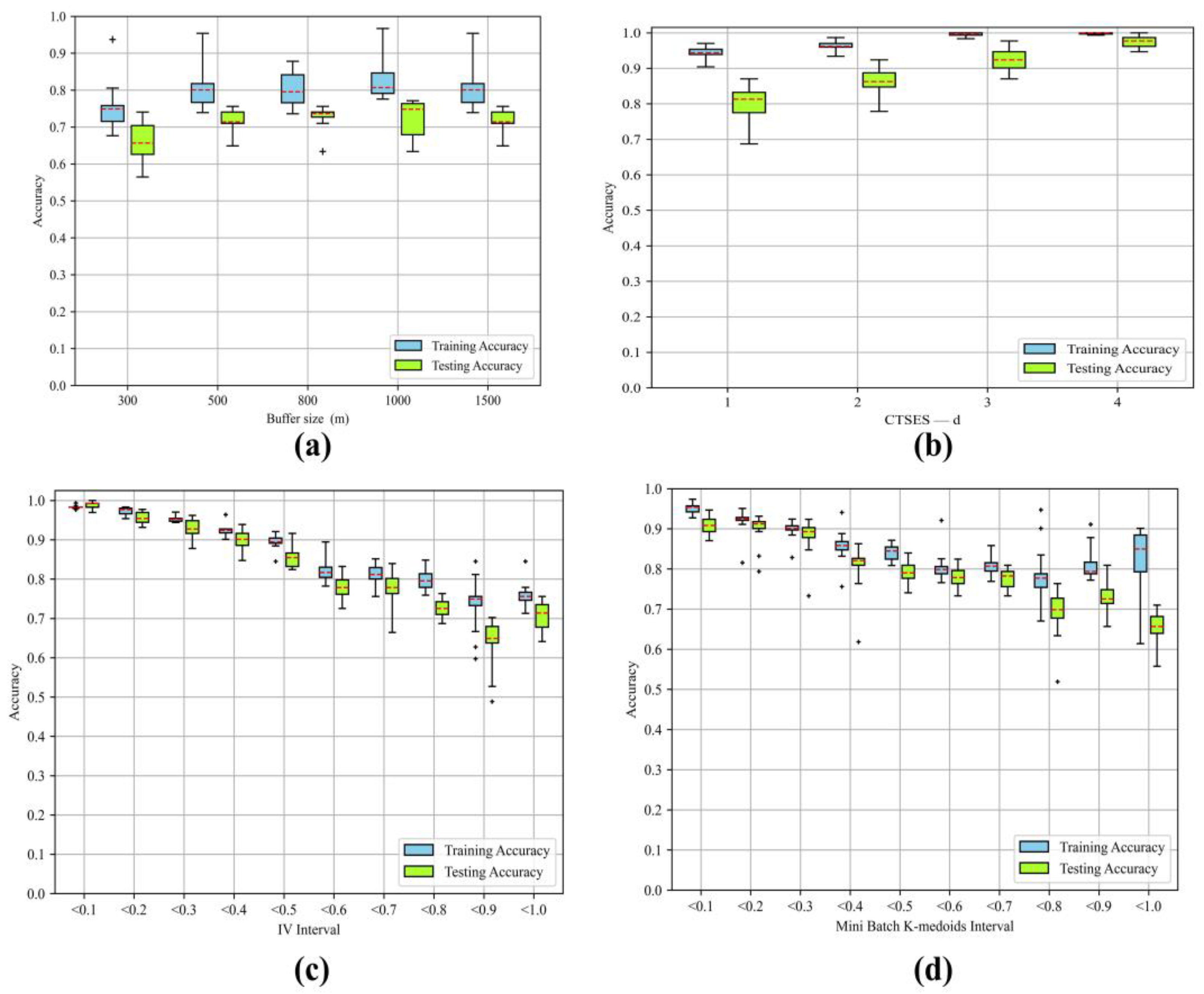
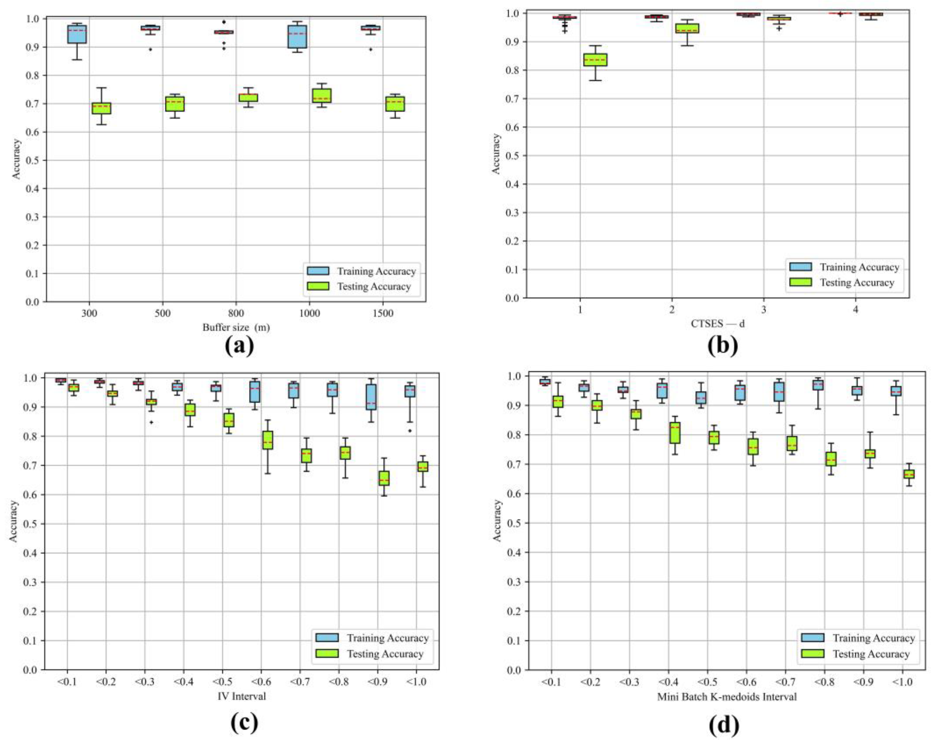
4.4.1. Model Accuracy of Four Absence Sampling Methods with Respective Sample Intervals
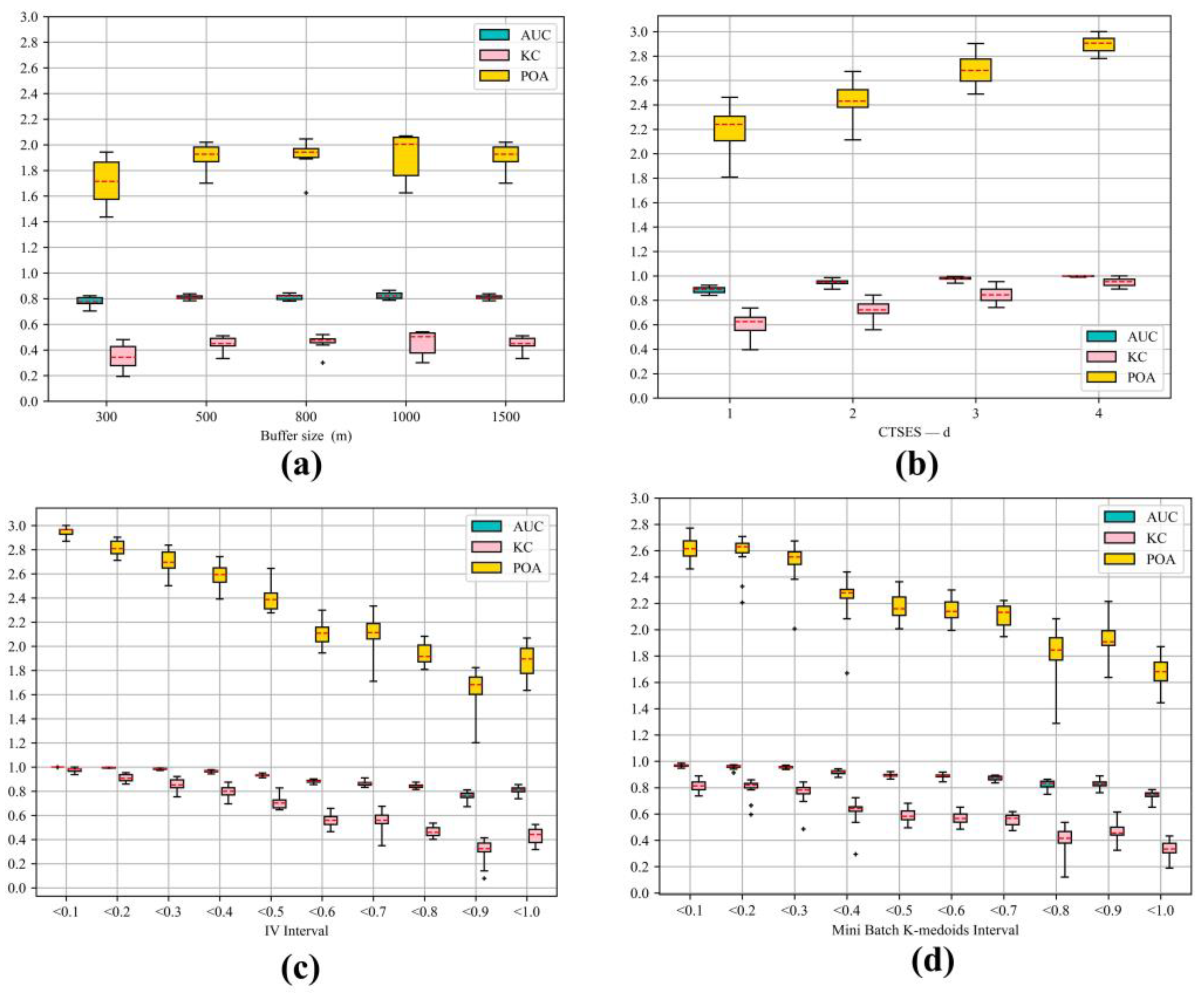
4.4.2. Model Comprehensive Predictive Performance of Four Absence Sampling Methods with Respective Sample Intervals
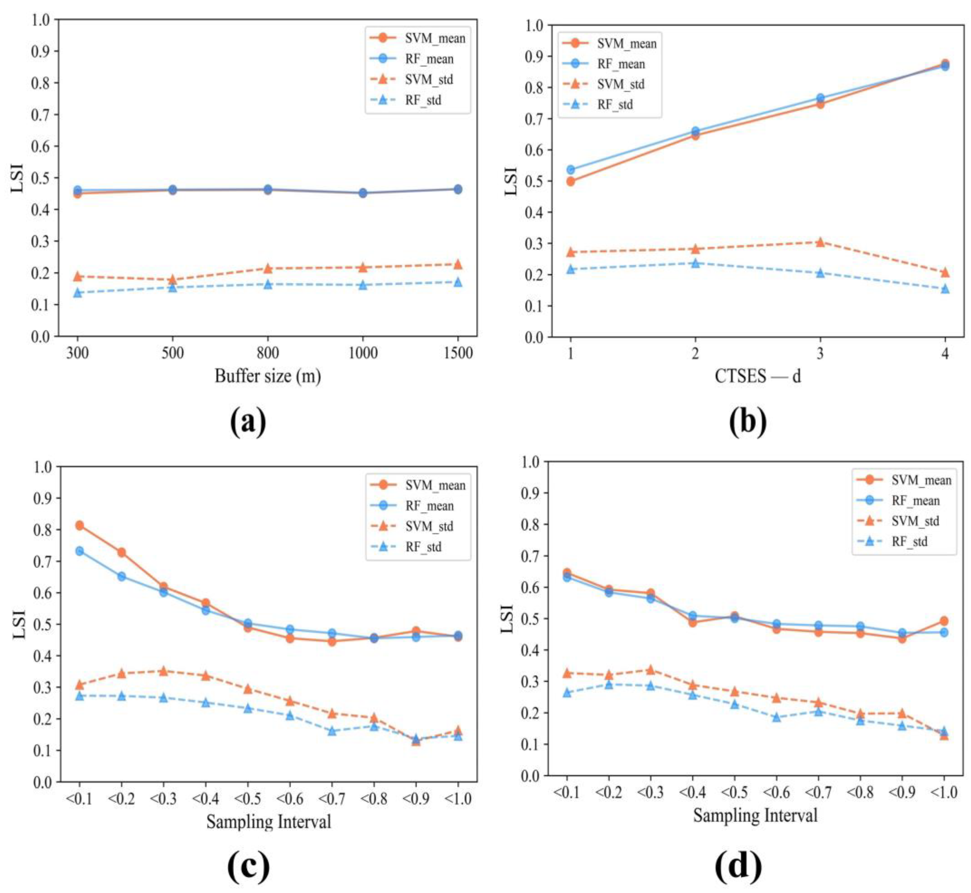
4.4.3. Model Susceptibility Distribution of Four Absence Sampling Methods with Respective Sample Intervals
4.4.4. Evaluation of the Integrative Sampling Model
5. Discussion
5.1. Effects of Absence Sampling Strategies and Sample Quality on LSM
5.2. Advantages of Integrative Sampling
6. Conclusions
Author Contributions
Funding
Data Availability Statement
Acknowledgments
Conflicts of Interest
References
- Wang, F.; Sassa, K. Landslide Simulation by a Geotechnical Model Combined with a Model for Apparent Friction Change. Phys. Chem. Earth Parts ABC 2010, 35, 149–161. [Google Scholar] [CrossRef]
- Adnan, M.S.G.; Rahman, M.S.; Ahmed, N.; Ahmed, B.; Rabbi, M.F.; Rahman, R.M. Improving Spatial Agreement in Machine Learning-Based Landslide Susceptibility Mapping. Remote Sens. 2020, 12, 3347. [Google Scholar] [CrossRef]
- Scaioni, M.; Longoni, L.; Melillo, V.; Papini, M. Remote Sensing for Landslide Investigations: An Overview of Recent Achievements and Perspectives. Remote Sens. 2014, 6, 9600–9652. [Google Scholar] [CrossRef]
- Zhao, C.; Lu, Z. Remote Sensing of Landslides—A Review. Remote Sens. 2018, 10, 279. [Google Scholar] [CrossRef]
- Mohan, A.; Singh, A.K.; Kumar, B.; Dwivedi, R. Review on Remote Sensing Methods for Landslide Detection Using Machine and Deep Learning. Trans. Emerg. Telecommun. Technol. 2021, 32, e3998. [Google Scholar] [CrossRef]
- Guzzetti, F.; Reichenbach, P.; Cardinali, M.; Galli, M.; Ardizzone, F. Probabilistic Landslide Hazard Assessment at the Basin Scale. Geomorphology 2005, 72, 272–299. [Google Scholar] [CrossRef]
- Corominas, J.; van Westen, C.; Frattini, P.; Cascini, L.; Malet, J.-P.; Fotopoulou, S.; Catani, F.; Van Den Eeckhaut, M.; Mavrouli, O.; Agliardi, F.; et al. Recommendations for the Quantitative Analysis of Landslide Risk. Bull. Eng. Geol. Environ. 2014, 73, 209–263. [Google Scholar] [CrossRef]
- Li, L.; Lan, H.; Guo, C.; Zhang, Y.; Li, Q.; Wu, Y. A Modified Frequency Ratio Method for Landslide Susceptibility Assessment. Landslides 2017, 14, 727–741. [Google Scholar] [CrossRef]
- Dou, J.; Xiang, Z.; Qiang, X.; Zheng, P.; Wang, X.; Su, A.; Liu, J.; Luo, W. Application and Development Trend of Machine Learning in Landslide Intelligent Disaster Prevention and Mitigation. Earth Sci. 2022. [Google Scholar]
- Merghadi, A.; Yunus, A.P.; Dou, J.; Whiteley, J.; ThaiPham, B.; Bui, D.T.; Avtar, R.; Abderrahmane, B. Machine Learning Methods for Landslide Susceptibility Studies: A Comparative Overview of Algorithm Performance. Earth-Sci. Rev. 2020, 207, 103225. [Google Scholar] [CrossRef]
- Nam, K.; Wang, F. An Extreme Rainfall-Induced Landslide Susceptibility Assessment Using Autoencoder Combined with Random Forest in Shimane Prefecture, Japan. Geoenvironmental Disasters 2020, 7, 6. [Google Scholar] [CrossRef]
- Nam, K.; Wang, F. The Performance of Using an Autoencoder for Prediction and Susceptibility Assessment of Landslides: A Case Study on Landslides Triggered by the 2018 Hokkaido Eastern Iburi Earthquake in Japan. Geoenvironmental Disasters 2019, 6, 19. [Google Scholar] [CrossRef]
- Huang, F.; Zhang, J.; Zhou, C.; Wang, Y.; Huang, J.; Zhu, L. A Deep Learning Algorithm Using a Fully Connected Sparse Autoencoder Neural Network for Landslide Susceptibility Prediction. Landslides 2020, 17, 217–229. [Google Scholar] [CrossRef]
- Huang, F.; Cao, Z.; Guo, J.; Jiang, S.-H.; Li, S.; Guo, Z. Comparisons of Heuristic, General Statistical and Machine Learning Models for Landslide Susceptibility Prediction and Mapping. Catena 2020, 191, 104580. [Google Scholar] [CrossRef]
- Huang, F.; Xiong, H.; Yao, C.; Catani, F.; Zhou, C.; Huang, J. Uncertainties of Landslide Susceptibility Prediction Considering Different Landslide Types. J. Rock Mech. Geotech. Eng. 2023. [Google Scholar] [CrossRef]
- Zhu, A.-X.; Miao, Y.; Yang, L.; Bai, S.; Liu, J.; Hong, H. Comparison of the Presence-Only Method and Presence-Absence Method in Landslide Susceptibility Mapping. Catena 2018, 171, 222–233. [Google Scholar] [CrossRef]
- Atkinson, P.M.; Massari, R. Generalised linear modelling of susceptibility to landsliding in the central apennines, Italy. Comput. Geosci. 1998, 24, 373–385. [Google Scholar] [CrossRef]
- Hearn, G.J.; Hart, A.B. Landslide Susceptibility Mapping: A Practitioner’s View. Bull. Eng. Geol. Environ. 2019, 78, 5811–5826. [Google Scholar] [CrossRef]
- Carrara, A.; Cardinali, M.; Guzzetti, F.; Reichenbach, P. Gis Technology in Mapping Landslide Hazard. In Geographical Information Systems in Assessing Natural Hazards; Carrara, A., Guzzetti, F., Eds.; Advances in Natural and Technological Hazards Research; Springer: Dordrecht, The Netherlands, 1995; pp. 135–175. ISBN 978-94-015-8404-3. [Google Scholar]
- Dou, J.; Yunus, A.P.; Merghadi, A.; Shirzadi, A.; Nguyen, H.; Hussain, Y.; Avtar, R.; Chen, Y.; Pham, B.T.; Yamagishi, H. Different Sampling Strategies for Predicting Landslide Susceptibilities Are Deemed Less Consequential with Deep Learning. Sci. Total Environ. 2020, 720, 137320. [Google Scholar] [CrossRef]
- Pourghasemi, H.R.; Kornejady, A.; Kerle, N.; Shabani, F. Investigating the Effects of Different Landslide Positioning Techniques, Landslide Partitioning Approaches, and Presence-Absence Balances on Landslide Susceptibility Mapping. Catena 2020, 187, 104364. [Google Scholar] [CrossRef]
- Zhu, A.-X.; Miao, Y.; Liu, J.; Bai, S.; Zeng, C.; Ma, T.; Hong, H. A Similarity-Based Approach to Sampling Absence Data for Landslide Susceptibility Mapping Using Data-Driven Methods. Catena 2019, 183, 104188. [Google Scholar] [CrossRef]
- Sameen, M.I.; Pradhan, B.; Bui, D.T.; Alamri, A.M. Systematic Sample Subdividing Strategy for Training Landslide Susceptibility Models. Catena 2020, 187, 104358. [Google Scholar] [CrossRef]
- Lucchese, L.V.; de Oliveira, G.G.; Pedrollo, O.C. Investigation of the Influence of Nonoccurrence Sampling on Landslide Susceptibility Assessment Using Artificial Neural Networks. Catena 2021, 198, 105067. [Google Scholar] [CrossRef]
- Pradhan, B.; Lee, S.; Buchroithner, M.F. A GIS-Based Back-Propagation Neural Network Model and Its Cross-Application and Validation for Landslide Susceptibility Analyses. Comput. Environ. Urban Syst. 2010, 34, 216–235. [Google Scholar] [CrossRef]
- Wang, H.; Zhang, L.; Luo, H.; He, J.; Cheung, R.W.M. AI-Powered Landslide Susceptibility Assessment in Hong Kong. Eng. Geol. 2021, 288, 106103. [Google Scholar] [CrossRef]
- Chang, Z.; Huang, J.; Huang, F.; Bhuyan, K.; Meena, S.R.; Catani, F. Uncertainty Analysis of Non-Landslide Sample Selection in Landslide Susceptibility Prediction Using Slope Unit-Based Machine Learning Models. Gondwana Res. 2023, 117, 307–320. [Google Scholar] [CrossRef]
- Xiao, C.; Tian, Y.; Shi, W.; Guo, Q.; Wu, L. A New Method of Pseudo Absence Data Generation in Landslide Susceptibility Mapping with a Case Study of Shenzhen. Sci. China Technol. Sci. 2010, 53, 75–84. [Google Scholar] [CrossRef]
- Hong, H.; Miao, Y.; Liu, J.; Zhu, A.-X. Exploring the Effects of the Design and Quantity of Absence Data on the Performance of Random Forest-Based Landslide Susceptibility Mapping. Catena 2019, 176, 45–64. [Google Scholar] [CrossRef]
- Rabby, Y.W.; Li, Y.; Hilafu, H. An Objective Absence Data Sampling Method for Landslide Susceptibility Mapping. Sci. Rep. 2023, 13, 1740. [Google Scholar] [CrossRef]
- Yuan, X.; Liu, C.; Nie, R.; Yang, Z.; Li, W.; Dai, X.; Cheng, J.; Zhang, J.; Ma, L.; Fu, X.; et al. A Comparative Analysis of Certainty Factor-Based Machine Learning Methods for Collapse and Landslide Susceptibility Mapping in Wenchuan County, China. Remote Sens. 2022, 14, 3259. [Google Scholar] [CrossRef]
- Zhao, B.; Ge, Y.; Chen, H. Landslide Susceptibility Assessment for a Transmission Line in Gansu Province, China by Using a Hybrid Approach of Fractal Theory, Information Value, and Random Forest Models. Environ. Earth Sci. 2021, 80, 441. [Google Scholar] [CrossRef]
- Xu, C.; Zhang, W.; Yi, Y.; Xu, Q. Landslide Susceptibility Mapping Using Logistic Regression Model Based on Information Value for the Region Along China-Thailand Railway from Saraburi to Sikhio, Thailand. In Proceedings of the IGARSS 2019—2019 IEEE International Geoscience and Remote Sensing Symposium, Yokohama, Japan, 31 July 2019; pp. 9650–9653. [Google Scholar]
- Zhao, Z.; Liu, Z.Y.; Xu, C. Slope Unit-Based Landslide Susceptibility Mapping Using Certainty Factor, Support Vector Machine, Random Forest, CF-SVM and CF-RF Models. Front. Earth Sci. 2021, 9, 589630. [Google Scholar] [CrossRef]
- Ji, J.; Zhou, Y.; Cheng, Q.; Jiang, S.; Liu, S. Landslide Susceptibility Mapping Based on Deep Learning Algorithms Using Information Value Analysis Optimization. Land 2023, 12, 1125. [Google Scholar] [CrossRef]
- Li, Y.; Deng, X.; Ji, P.; Yang, Y.; Jiang, W.; Zhao, Z. Evaluation of Landslide Susceptibility Based on CF-SVM in Nujiang Prefecture. Int. J. Environ. Res. Public. Health 2022, 19, 14248. [Google Scholar] [CrossRef]
- Huang, F.; Yin, K.; Huang, J.; Gui, L.; Wang, P. Landslide Susceptibility Mapping Based on Self-Organizing-Map Network and Extreme Learning Machine. Eng. Geol. 2017, 223, 11–22. [Google Scholar] [CrossRef]
- Kaboutari, A.; Bagherzadeh, J.; Kheradmand, F. An Evaluation of Two-Step Techniques for Positive-Unlabeled Learning in Text Classification. Int. J. Comput. Appl. Technol. Res. 2014, 3, 592–594. [Google Scholar] [CrossRef]
- Huang, F.; Cao, Z.; Jiang, S.-H.; Zhou, C.; Huang, J.; Guo, Z. Landslide Susceptibility Prediction Based on a Semi-Supervised Multiple-Layer Perceptron Model. Landslides 2020, 17, 2919–2930. [Google Scholar] [CrossRef]
- Yao, J.; Qin, S.; Qiao, S.; Liu, X.; Zhang, L.; Chen, J. Application of a Two-Step Sampling Strategy Based on Deep Neural Network for Landslide Susceptibility Mapping. Bull. Eng. Geol. Environ. 2022, 81, 148. [Google Scholar] [CrossRef]
- Chang, Z.; Du, Z.; Zhang, F.; Huang, F.; Chen, J.; Li, W.; Guo, Z. Landslide Susceptibility Prediction Based on Remote Sensing Images and GIS: Comparisons of Supervised and Unsupervised Machine Learning Models. Remote Sens. 2020, 12, 502. [Google Scholar] [CrossRef]
- Zhu, L.P.; Chen, R.; Zeng, J.W.; Liao, S.B.; Yang, Z.L. Main structural characteristics of Yanshanian in Shengzhou area of Yuyao-Lishui fault zone (in Chinese). Chin. Geol. Surv. 2018, 5, 49–57. [Google Scholar]
- Chen, L.F. Study on the Activity of NE Trending Faults along the Coast of Zhejiang Province (in Chinese). Master’s Thesis, Zhejiang University, Hangzhou, China, 2010. [Google Scholar]
- Wang, F.; Chen, Y.; Peng, X.; Zhu, G.; Yan, K.; Ye, Z. The Fault-Controlled Chengtian Landslide Triggered by Rainfall on 20 May 2021 in Songyang County, Zhejiang Province, China. Landslides 2022, 19, 1751–1765. [Google Scholar] [CrossRef]
- Fabbri, A.G.; Chung, C.-J.F.; Cendrero, A.; Remondo, J. Is Prediction of Future Landslides Possible with a GIS? Nat. Hazards 2003, 30, 487–503. [Google Scholar] [CrossRef]
- Yi, Y.; Zhang, Z.; Zhang, W.; Jia, H.; Zhang, J. Landslide Susceptibility Mapping Using Multiscale Sampling Strategy and Convolutional Neural Network: A Case Study in Jiuzhaigou Region. Catena 2020, 195, 104851. [Google Scholar] [CrossRef]
- Xi, C.; Han, M.; Hu, X.; Liu, B.; He, K.; Luo, G.; Cao, X. Effectiveness of Newmark-Based Sampling Strategy for Coseismic Landslide Susceptibility Mapping Using Deep Learning, Support Vector Machine, and Logistic Regression. Bull. Eng. Geol. Environ. 2022, 81, 174. [Google Scholar] [CrossRef]
- Hu, J.; Xu, K.; Wang, G.; Liu, Y.; Khan, M.A.; Mao, Y.; Zhang, M. A Novel Landslide Susceptibility Mapping Portrayed by OA-HD and K-Medoids Clustering Algorithms. Bull. Eng. Geol. Environ. 2021, 80, 765–779. [Google Scholar] [CrossRef]
- Pokharel, B.; Althuwaynee, O.F.; Aydda, A.; Kim, S.-W.; Lim, S.; Park, H.-J. Spatial Clustering and Modelling for Landslide Susceptibility Mapping in the North of the Kathmandu Valley, Nepal. Landslides 2021, 18, 1403–1419. [Google Scholar] [CrossRef]
- Kim, J.-C.; Lee, S.; Jung, H.-S.; Lee, S. Landslide Susceptibility Mapping Using Random Forest and Boosted Tree Models in Pyeong-Chang, Korea. Geocarto Int. 2018, 33, 1000–1015. [Google Scholar] [CrossRef]
- Dou, J.; Yunus, A.P.; Tien Bui, D.; Merghadi, A.; Sahana, M.; Zhu, Z.; Chen, C.-W.; Khosravi, K.; Yang, Y.; Pham, B.T. Assessment of Advanced Random Forest and Decision Tree Algorithms for Modeling Rainfall-Induced Landslide Susceptibility in the Izu-Oshima Volcanic Island, Japan. Sci. Total Environ. 2019, 662, 332–346. [Google Scholar] [CrossRef]
- Dou, J.; Yunus, A.P.; Bui, D.T.; Merghadi, A.; Sahana, M.; Zhu, Z.; Chen, C.-W.; Han, Z.; Pham, B.T. Improved Landslide Assessment Using Support Vector Machine with Bagging, Boosting, and Stacking Ensemble Machine Learning Framework in a Mountainous Watershed, Japan. Landslides 2020, 17, 641–658. [Google Scholar] [CrossRef]
- Yao, X.; Tham, L.G.; Dai, F.C. Landslide Susceptibility Mapping Based on Support Vector Machine: A Case Study on Natural Slopes of Hong Kong, China. Geomorphology 2008, 101, 572–582. [Google Scholar] [CrossRef]
- Hong, H.; Pradhan, B.; Jebur, M.N.; Bui, D.T.; Xu, C.; Akgun, A. Spatial Prediction of Landslide Hazard at the Luxi Area (China) Using Support Vector Machines. Environ. Earth Sci. 2015, 75, 40. [Google Scholar] [CrossRef]
- Marjanović, M.; Kovačević, M.; Bajat, B.; Voženílek, V. Landslide Susceptibility Assessment Using SVM Machine Learning Algorithm. Eng. Geol. 2011, 123, 225–234. [Google Scholar] [CrossRef]
- Wang, H.; Zhang, L.; Yin, K.; Luo, H.; Li, J. Landslide Identification Using Machine Learning. Geosci. Front. 2021, 12, 351–364. [Google Scholar] [CrossRef]
- Beauchamp, K.A.; Bowman, G.R.; Lane, T.J.; Maibaum, L.; Haque, I.S.; Pande, V.S. MSMBuilder2: Modeling Conformational Dynamics on the Picosecond to Millisecond Scale. J. Chem. Theory Comput. 2011, 7, 3412–3419. [Google Scholar] [CrossRef]


| Conditioning Factor | Variable Type | Spatial Resolution (m) | Production Time (year) | Data Source |
|---|---|---|---|---|
| Altitude | Continuous | 30 | 2009 | ASTER GDEM 30M |
| Slope | Continuous | 30 | 2009 | Derived from DEM |
| Slope aspect | Continuous | 30 | 2009 | Derived from DEM |
| Plan curvature | Continuous | 30 | 2009 | Derived from DEM |
| Profile curvature | Continuous | 30 | 2009 | Derived from DEM |
| TRI | Continuous | 30 | 2009 | Derived from DEM |
| TWI | Continuous | 30 | 2009 | Derived from DEM |
| STI | Continuous | 30 | 2009 | Derived from DEM |
| Lithology | Discrete | 30 | 2019 | [41] |
| Distance to faults | Continuous | 30 | 2019 | [41] |
| Soil type | Discrete | 30 | 2005 | https://www.resdc.cn/ (accessed on 1 May 2022) |
| Annual rainfall | Continuous | 30 | 2000–2021 | http://data.cma.cn/ (accessed on 1 May 2022) |
| Distance to stream | Continuous | 30 | 2021 | https://lbs.amap.com/ (accessed on 1 May 2022) |
| Distance to road | Continuous | 30 | 2021 | https://lbs.amap.com/ (accessed on 1 May 2022) |
| Land use | Discrete | 30 | 2020 | https://www.resdc.cn/ (accessed on 1 May 2022) |
| NDVI | Continuous | 30 | 2021 | Landsat8 |
| Factor | VIF | TOL |
|---|---|---|
| Elevation | 2.613 | 0.383 |
| Slope | 1.685 | 0.594 |
| Aspect | 1.105 | 0.905 |
| Profile curvature | 2.010 | 0.498 |
| Plane curvature | 2.087 | 0.479 |
| TRI | 1.558 | 0.642 |
| TWI | 2.090 | 0.478 |
| STI | 1.118 | 0.894 |
| NDVI | 1.143 | 0.875 |
| Lithology | 1.223 | 0.818 |
| Rainfall | 1.570 | 0.637 |
| Distance to faults | 1.028 | 0.972 |
| Distance to rivers | 1.172 | 0.854 |
| Distance to roads | 1.613 | 0.620 |
| Land use | 1.032 | 0.969 |
| Soil type | 1.350 | 0.740 |
| Factor | Class | No. of Landslides | No. of Pixels in Domain | IV |
|---|---|---|---|---|
| Altitude (m) | 34–400 | 65 | 400,676 | 0.154 |
| 301–600 | 105 | 529,308 | 0.355 | |
| 601–900 | 40 | 424,249 | −0.389 | |
| 901–1200 | 7 | 191,726 | −1.338 | |
| 1201–1492 | 0 | 13,793 | 0.000 | |
| Slope (°) | 0–10 | 35 | 285,800 | −0.128 |
| 10.1–20 | 75 | 353,914 | 0.421 | |
| 20.1–30 | 60 | 484,962 | −0.117 | |
| 30.1–40 | 37 | 339,129 | −0.243 | |
| 40.1–50 | 10 | 84,504 | −0.162 | |
| >50 | 0 | 5759 | 0.000 | |
| Aspect (°) | 0 | 0 | 5939 | 0.000 |
| 0–22.5 | 11 | 89,012 | −0.118 | |
| 22.6–67.5 | 34 | 202,755 | 0.187 | |
| 67.6–112.5 | 32 | 216,747 | 0.059 | |
| 112.6–157.5 | 35 | 202,523 | 0.217 | |
| 157.6–202.5 | 30 | 178,953 | 0.186 | |
| 202.6–247.5 | 24 | 182,953 | −0.059 | |
| 247.6–292.5 | 26 | 194,308 | −0.039 | |
| 292.6–337.5 | 16 | 192,853 | −0.517 | |
| 337.6–360 | 9 | 88,025 | −0.308 | |
| Plane curvature | (−9.487–−1.297) | 7 | 90,832 | −0.591 |
| (−1.296–−0.355) | 57 | 358,239 | 0.134 | |
| (−0.354–0.370) | 89 | 646,319 | −0.010 | |
| (−0.371–1.239) | 56 | 354,515 | 0.127 | |
| (1.240–8.994) | 8 | 109,847 | −0.647 | |
| Profile curvature | (−10.848–−1.643) | 4 | 78,385 | −1.003 |
| (−1.642–−0.482) | 36 | 318,609 | −0.208 | |
| (−0.481–0.412) | 91 | 696,850 | −0.063 | |
| (0.413–1.574) | 70 | 376,172 | 0.291 | |
| (1.575–11.940) | 16 | 89,736 | 0.248 | |
| TWI | (2.354–4.686) | 85 | 656,862 | −0.072 |
| (4.687–6.410) | 69 | 524,863 | −0.057 | |
| (6.411–8.742) | 40 | 250,590 | 0.137 | |
| (8.743–12.392) | 17 | 92,287 | 0.281 | |
| (12.393–28.209) | 6 | 29,466 | 0.381 | |
| TRI | (0.111–0.294) | 23 | 85,999 | 0.654 |
| (0.295–0.419) | 45 | 246,752 | 0.271 | |
| (0.420–0.498) | 80 | 535,396 | 0.071 | |
| (0.499–0.578) | 52 | 531,083 | −0.351 | |
| (0.579–0.889) | 17 | 208,097 | −0.532 | |
| STI | (0–3.0) | 84 | 715,531 | −0.170 |
| (3.1–12.0) | 64 | 586,030 | −0.242 | |
| (12.1–15.0) | 11 | 50,604 | 0.446 | |
| (15.1 -50.0) | 31 | 140,393 | 0.462 | |
| (>50.0) | 27 | 75,298 | 0.947 | |
| NDVI | (−0.184–0.077) | 32 | 214,619 | 0.069 |
| (0.078–0.161) | 54 | 270,357 | 0.362 | |
| (0.162–0.239) | 66 | 361,211 | 0.273 | |
| (0.240–0.316) | 49 | 403,597 | −0.136 | |
| (0.317–0.486) | 16 | 309,958 | −0.991 | |
| Rainfall (mm/year) | 1488–1497 | 33 | 118,347 | 0.695 |
| 1498–1528 | 33 | 211,130 | 0.116 | |
| 1529–1552 | 28 | 398,437 | −0.683 | |
| 1553–1575 | 70 | 494,390 | 0.018 | |
| 1576–1611 | 53 | 337,453 | 0.121 | |
| Distance to rivers (m) | 0–50 | 39 | 169,598 | 0.503 |
| 51–150 | 79 | 327,307 | 0.551 | |
| 151–300 | 52 | 338,629 | 0.099 | |
| 301–600 | 39 | 498,642 | −0.576 | |
| >600 | 8 | 175,619 | −1.116 | |
| Distance to roads (m) | 0–200 | 66 | 222,151 | 0.759 |
| 201–400 | 21 | 147,406 | 0.024 | |
| 401–600 | 8 | 119,129 | −0.728 | |
| 601–800 | 13 | 102,609 | −0.094 | |
| >800 | 109 | 968,500 | −0.212 | |
| Distance to faults (m) | 0–200 | 17 | 146,962 | −0.185 |
| 201–500 | 21 | 213,815 | −0.348 | |
| 501–1000 | 61 | 318,946 | 0.318 | |
| 1001–1500 | 37 | 256,177 | 0.037 | |
| >1500 | 81 | 623,895 | −0.069 | |
| Land use | Residential | 3 | 42,047 | −0.668 |
| Bare land | 0 | 2209 | 0.000 | |
| Forest | 155 | 1,264,284 | −0.126 | |
| Water body | 1 | 12,156 | −0.525 | |
| Farmland | 56 | 216,100 | 0.622 | |
| Grassland | 2 | 21,548 | −0.405 | |
| Soil type | Rock | 0 | 9137 | 0.000 |
| Brown earth | 3 | 78,111 | −1.287 | |
| Paddy soil | 20 | 170,108 | −0.168 | |
| Limestone soil | 1 | 4313 | 0.511 | |
| Red earth | 179 | 1,011,069 | 0.241 | |
| Yellow earth | 14 | 288,375 | −1.053 | |
| Lithology | Sandstone | 10 | 153,095 | −0.756 |
| Quartz sandstone | 47 | 179,684 | 0.631 | |
| Gneiss | 18 | 56,402 | 0.830 | |
| Tuff | 38 | 373,449 | −0.313 | |
| Rhyolite | 86 | 679,184 | −0.094 | |
| Quaternary alluvium | 3 | 78,859 | −1.297 | |
| Granodiorite Porphyry | 15 | 38,986 | 1.017 |
| Predictive Model | Presence: Absence | Training Accuracy | Testing Accuracy | AUC | KC | POA | Susceptibility Mean | Susceptibility SD |
|---|---|---|---|---|---|---|---|---|
| SVM | 1:1 | 0.90 | 0.77 | 0.89 | 0.55 | 2.13 | 0.52 | 0.29 |
| 3:7 | 0.93 | 0.81 | 0.87 | 0.56 | 2.06 | 0.36 | 0.28 | |
| RF | 1:1 | 0.96 | 0.86 | 0.92 | 0.73 | 2.46 | 0.56 | 0.23 |
| 3:7 | 0.97 | 0.83 | 0.91 | 0.60 | 2.15 | 0.39 | 0.21 |
Disclaimer/Publisher’s Note: The statements, opinions and data contained in all publications are solely those of the individual author(s) and contributor(s) and not of MDPI and/or the editor(s). MDPI and/or the editor(s) disclaim responsibility for any injury to people or property resulting from any ideas, methods, instructions or products referred to in the content. |
© 2023 by the authors. Licensee MDPI, Basel, Switzerland. This article is an open access article distributed under the terms and conditions of the Creative Commons Attribution (CC BY) license (https://creativecommons.org/licenses/by/4.0/).
Share and Cite
Fu, Z.; Wang, F.; Dou, J.; Nam, K.; Ma, H. Enhanced Absence Sampling Technique for Data-Driven Landslide Susceptibility Mapping: A Case Study in Songyang County, China. Remote Sens. 2023, 15, 3345. https://doi.org/10.3390/rs15133345
Fu Z, Wang F, Dou J, Nam K, Ma H. Enhanced Absence Sampling Technique for Data-Driven Landslide Susceptibility Mapping: A Case Study in Songyang County, China. Remote Sensing. 2023; 15(13):3345. https://doi.org/10.3390/rs15133345
Chicago/Turabian StyleFu, Zijin, Fawu Wang, Jie Dou, Kounghoon Nam, and Hao Ma. 2023. "Enhanced Absence Sampling Technique for Data-Driven Landslide Susceptibility Mapping: A Case Study in Songyang County, China" Remote Sensing 15, no. 13: 3345. https://doi.org/10.3390/rs15133345
APA StyleFu, Z., Wang, F., Dou, J., Nam, K., & Ma, H. (2023). Enhanced Absence Sampling Technique for Data-Driven Landslide Susceptibility Mapping: A Case Study in Songyang County, China. Remote Sensing, 15(13), 3345. https://doi.org/10.3390/rs15133345