Abstract
Recently, atmospheric perturbations residing over around epicenters of forthcoming earthquakes were remotely sensed by the multiple instruments of the MVP-LAI (Monitoring of Vibrations and Perturbations in Lithosphere, Atmosphere and Ionosphere) system. In this study, we found another way and proposed a theory for the evolution of the perturbations in the atmosphere from the aspect of numerical simulation. We started from the fundamental hydromechanics equations for the perturbations based on the atmospheric dynamics in the cylindrical symmetric coordinate to solve their analytical solution. The solution shows that a persistent vibration at the bottom of the cylindrical symmetric coordinate tends to decay exponentially with along altitude. In other words, a persistent ground vibration in a wide area can rapidly evolve into small-scale perturbations in the atmosphere. The preliminary theoretical model in this study shows the kernel concept for the coupling of geospheres.
1. Introduction
The coupling of the lithosphere, atmosphere, and ionosphere (LAI) has been widely reported in previous studies [1,2,3,4,5,6,7,8,9,10,11,12,13,14,15,16,17]. Four promising channels have been proposed and examined by numerous geophysical parameters during hazard events [16,18,19,20]. The chemical channel suggests that the total electron contents (TECs) in the ionosphere can be changed by variations in the atmospheric contents near the Earth’s surface mainly due to gas released from the underground [21,22]. The conductivity channel indicates the ionosphere can be heated by the upward lighting due to the enhancement of the conductivity near the Earth’s surface [23,24,25]. The TEC can also be changed by the acoustic and gravity waves (i.e., the acoustic-gravity channel) [26,27,28,29,30,31,32,33,34,35]. Changes in TECs exhibit period characteristics longer than ~5 min that is probably related to the atmospheric gravity waves [36,37]. Generations of the gravity waves are mainly referred to variations in temperature near the Earth’s surface [38,39,40,41,42,43,44]. In contrast, changes of TECs with period characteristics shorter than ~5 min are probably caused by the acoustic waves [45,46]. The acoustic waves mainly originate from the ground vibrations particularly for the Rayleigh waves and propagate upward with sonic velocity from the Earth’s surface to the ionosphere [2,6,11,14,31,47]. In terms of the electromagnetic emission channel, enhancements of the electromagnetic field at a particular frequency band of ~0.01 Hz can change the ionosphere, accordingly [48,49]. Seismo-anomalous phenomena have been observed in the LAI. The four potential channels (i.e., radiation gases for the chemical channel, current and/or water for the conductivity channel, geothermal temperature variations for the acoustic-gravity channel, and the geomagnetic anomaly for the emission channel) have been proposed to explain the seismo-TEC anomalies triggered by changes in the lithosphere. (see the references mentioned in above). However, the causal mechanisms for the seismo-LAI coupling remain unclear. Chen et al. [50] retrieved seismo-crustal deformation from the long-term crustal displacement data. The results show that seismo-crustal deformation for earthquake preparation covering a larger area that is hereafter confirmed by the study [51] reported in 2020. The seismo-deformation and vibrations begin few days before earthquakes [51,52,53,54,55]. Moreover, numerous studies have shown that the lithosphere-atmosphere-ionosphere coupling phenomenon can be observed before earthquake [1,2,3,4].Those observation results suggest that the seismo-ground vibrations can be promising sources triggering acoustic waves upward propagating and driving changes in atmosphere and TEC via the acoustic-gravity channel that have to be examine.
Chen et al. [52] analyzed crustal displacements and/or deformation data from the seismometers and ground-based GNSS (Global Navigation Satellite System) receivers associated with major earthquakes. Seismo-ground vibrations with amplitude of 0.1 m at frequencies ranged mainly between 8 × 10⁻⁵ Hz and 2 × 10⁻⁴ Hz in a wide area with a radius of epicentral distance >200 km. Chen et al. [56] found that the frequencies where the ground vibration amplitudes enhanced were not stable but tended to be high at (>10−2 Hz) with the approaching of forthcoming earthquakes. Meanwhile, the frequencies can be a resonant phenomenon as natural frequencies before failure of a grant size of rocks that can be estimated by changes in seismicity [56]. To examine whether the seismo-ground vibrations can excite acoustic waves deriving changes in atmosphere and TECs or not, Chen et al. [57] established an instrumental array in Sichuan, China for monitoring the vibrations and perturbations in the lithosphere, atmosphere and ionosphere (MVP-LAI). Ground vibrations and TECs share the frequency of ~0.005 Hz before the earthquakes due to that the atmospheric resonance was attributed to the persistent lithospheric vibrations in a wide frequency band [58]. Chen et al. [59] reported that a resonant LAI coupling is existence even if the amplitude of vibrations in the lithosphere is small.
The previous studies showed the observational evidence of the persistent lithospheric vibrations inducing disturbance and wave in the atmosphere. However, a possible mathematical proof does not yet exist, which motivates us to derive the theoretical solution of the wave evolution due to the persistent lithospheric vibrations. Some previous studies on numeric simulations have been performed [60,61,62,63,64,65,66,67,68,69,70,71,72]. Mikhailenko et al. [60] developed a numerical–analytical algorithm to simulate the propagation of seismic and acoustic-gravity waves within the limits of a heterogeneous Earth–Atmosphere model. The algorithm is based on the integral Laguerre transform with respect to time and tested for simple models of an elastic half-space that borders on the atmosphere. Kherani et al. [61] simulated the atmosphere and ionospheric anomalies for the Tohoku-Oki tsunami and found that the Tsunami-Atmosphere-Ionosphere (TAI) coupling mechanism via acoustic-gravity waves (AGWs) was explored theoretically using the TAI-coupled model. Brissaund et al. [62] introduced a finite difference in the time domain (FDTD) approach to stimulate interactions between lithosphere and atmosphere. Carbone et al. [68] used the Wentzel-Kramers-Brillouin (WKB) approach to simulate the atmospheric fluctuations excited by a generic seismic event on the top of the first layer of the atmosphere, and estimated its dispersion relation as a function of the characteristic parameters of the earthquake. Matsumura et al. [72] simulated the atmospheric perturbations observed at 300-km altitude just after the 2011 off the Pacific coast of Tohoku Earthquake, and the results showed remarkable agreement with the observed TEC oscillations qualitatively. Most of the previous studies simulate the atmospheric acoustic or gravity waves triggered by a point source [60,61,62,63,64,65,66,67,68,69,70,71,72,73,74,75,76,77], while the ground vibrations are typically observed in a wide area [52]. Therefore, the innovation of the simulation in this study considers the persistent variation in a wide area. We quantitatively analyze atmospheric perturbations triggered by persistent lithospheric vibrations below a height of 100 km based on the numerical simulation results.
2. Perturbation Equations in the Cylindrical Symmetric Coordinates and its Numerical Solution
As we all know, air is a typical fluid, so the dynamical properties in atmosphere can be described by the physical quantities such as atmospheric pressure, air density and flow velocities, and the physical evolution process can be derived by hydromechanics equations. In the cylinder coordinate, the equations of atmospheric dynamics are given by
where , , and are atmospheric pressure, air density, viscous forces and (radial, tangential and vertical) velocity of the fluid respectively. is acceleration of gravity ( is the earth radius, is the mass of earth, and is the gravitational constant), and the earth rotates with angular velocity ( is the angular velocity of the earth’s rotation, is dimension, and is the Coriolis parameter).
The equation of continuity, thermodynamical equation and the water vapor equation are
where is the amount of heat per unit mass of air per unit time received from the outside, is the temperature of air, is specific heat of air at constant pressure, and are specific humidity and the amount of water vapor per unit mass of wet air obtained from the outside world per unit time. In hydromechanics, we set
For the sake of simplicity, the earth rotation effect and viscous effect of fluid are ignored, so . We also ignore the water vapor Equation (6) and the exchange of heat between air and the outside of system (), and assume all physical quantities in the work have cylindrical symmetry, so that above equations are simplified as:
We consider the air as perfect gas, so it satisfy the state equation:
with . Under the condition of no wind, let’s consider a perturbation with frequency , so the physical funtions are set as the form: , , , , with as mark of perturbation. We can get
with . Therefore, we get the perturbation equations as follows
From Equations (14), (15) and (17), we can derive , and by and its derivative. By using the ansatz , Equation (16) is rewritten as
where is a constant of separating variables.
Now, let’s try to solve . As , we find , but it is a trivial solution because at infinity (). It means that can not vanish () in this work, and the solution is with because the boundary condition at infinity, (where and are the Berssel function of the first kind and the second kind respectively). For the sake of simplificity, it is assumed that atmosphere pressure satisfy the relation
where the parameter is the atmosphere scale height, and is atmospheric pressure near the ground. Finally, we obtain the numerical solution of perturbation equations as follows:
The physical solutions should be the real parts of solutions, so we have
We have rewritten the z- component of perturbation physical quantities as , , and , whose analytical forms are given in Equations (20)–(23).
3. Results and Discussion
The specific parameters are substituited into above formulas, and we investigate the function propreties with different radius and altitudes. To show the evolution of the perturbations from ground to upper atmosphere, we choose , and substitute the parameters into above equations.
The signals with a frequency of ~ Hz due to the ground vibrations within a wide area with a radius larger than ~ km (Figure 1) reach the upper atmosphere at 100 km altitude (Figure 2). The air pressure and density perturbations attenuate significantly with height (Figure 2a,b). The results suggest the feasibility of ground vibrations propagating into the upper atmosphere. Moreover, we can also find that the propagation velocities ( and ) in upper atmosphere is faster than those near the ground (Figure 2c,d), which indicate that the perturbations propagate easier at the lower pressure and density atmosphere. Accordingly, the upper atmosphere is an ideal signal transfer medium for the warning of natural disasters, such as volcanic eruption and earthquakes [77].
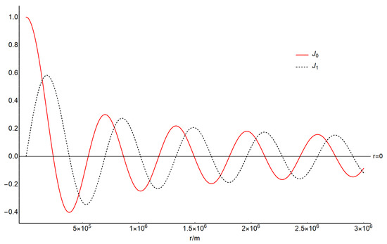
Figure 1.
Two Bessel Function J0 (CLr) and J1 (CLr), with different values of r.
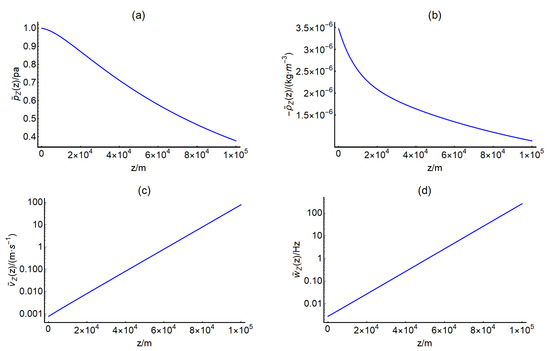
Figure 2.
The z-component of the pressure perturbation (a), air density perturbation (b), radial and vertical velocity perturbation (c) and angular frequency (d).
The lithosphere-atmosphere coupling has been observed and widely reported in many previous studies. The coupling phenomena can be detected during earthquakes and volcanic eruptions [4,11,58,59,60,78]. However, the coupling phenomena too complex to be simulated comprehensively. Therefore, in this study, we stand on the ground and started from solving the classical hydromechanics equations to deal with the complex mechanism for coupling. We calculated the numerical solution of the disturbance equations in the cylindrical symmetric coordinate to understand the possible effect of the persistent lithospheric vibrations on the upper atmosphere, which is a preliminary result for explaining the possible relation between the vibration signals on the ground and those in the atmosphere above. The solution reveals that the persistent vibrations in a wide area on the ground (>105 km2, mainly corresponding to the area of Sichuan Province, China (https://www.sc.gov.cn/, accessed on 8 March 2022) is capable of decaying rapidly in the z direction of the cylinder. The rapid decay of large disturbance agrees with the observational evidences of a large disturbances tend to evolve into finer-scale in the atmosphere [75,76].
In fact, the ground vibrations are recognizable before earthquake [51,56,59], and they can propagate upward to change the air pressure in the atmosphere and TEC in the ionosphere [4,11,59]. Essential parameters in different spheres can be recorded by corresponding instruments. Liu et al. [11] showed that the magnetometer can observed changes in the ionosphere current at 100 km in altitude. The HF Doppler sounding can detect changes at 200 km in altitude. The ground-based GNSS receivers can monitor changes in TEC.
Previous studies simulate the atmospheric acoustic or gravity waves triggered by a point source [75,76,77]. The new idea of the simulation in this study is considering the persistent variation in a wide area. In other words, the numerical results reveal that persistent ground vibrations in a wide area are possible to evolves into small-scale perturbations in the atmosphere [76]. Figure 2c shows that vertical velocity gradually increases with height, and finally reach 100 m/s at 100 km altitude. We compare the simulation result with the observation from Liu et al. [11]. Their observational results show the velocity of acoustic wave triggered from ground increased with height and up to 400 m/s at 100 km altitude. The simulation and observational results yield similar characteristics, while little discrepancy of velocity between them may be due to the complexity of nature we have not considered at present. For instance, the waves or disturbances evolve nonlinearly [46,76] and interact with the background wind flow [77,78], which relates to numerous effects such as Coriolis’s force, viscosity of air, nonlinear wave-to-wave interaction, dynamics etc.
The preliminary analytical simulation is based on the conclusions of observational evidence from previous studies. In fact, we show the possibility of waves evolving from the lithosphere to the atmosphere. We understand that actual situation can reduce the possibility. However, the reduction of the possibility cannot change the fact of the waves propagating from the lithosphere to the atmosphere. Of course, the calculation in the frequency domain can be extended and transformed to the time domain for the further visualization application.
4. Conclusions
The analytical solution of perturbations in the hydromechanics equations in the cylindrical symmetric coordinate was solved. This is a preliminary theoretical model. The solution preliminarily proves the observational evidence that ground vibrations of wide area with a radius larger than ~102 km in the lithosphere can propagate into the atmosphere and evolve there. The vibrations are capable of decaying rapidly with the altitude. The solution is quite challenged to be found from the fundamental equations of atmospheric disturbances and dynamics for the geospheres’ coupling that is complex. Therefore, the preliminary theoretical model in this study here shows the kernel concept, and of course it will be improved in several aspects in the future.
Author Contributions
Conceptualization, K.L. and C.-H.C.; methodology, K.L.; software, K.L.; validation, Z.X.; formal analysis, K.L. and C.-H.C.; investigation, K.L. and C.-H.C.; writing—original draft preparation, K.L. and C.-H.C.; writing—review and editing, Z.M., L.D., X.Z. and Y.G.; visualization, K.L., Z.X. and Z.M.; funding acquisition, K.L. All authors have read and agreed to the published version of the manuscript.
Funding
This research was funded by National Natural Science Foundation of China (NNSFC), grant number 42230207, and the Basal Research Fund of Institute of Earthquake Forecasting, China Earthquake Administration, grant number CEAIEF20230401.
Data Availability Statement
Not applicable.
Conflicts of Interest
The authors declare no conflict of interest.
References
- Afraimovich, E.L.; Perevalova, N.P.; Plotnikov, A.; Uralov, A. The shock-acoustic waves generated by earthquakes. Ann. Geophys. 2001, 19, 395–409. [Google Scholar] [CrossRef]
- Artru, J.; Farges, T.; Lognonné, P. Acoustic waves generated from seismic surface waves: Propagation properties determined from Doppler sounding observations and normal-mode modelling. Geophys. J. Int. 2004, 158, 1067–1077. [Google Scholar] [CrossRef]
- Calais, E.; Bernard Minster, J.; Hofton, M.; Hedlin, M. Ionospheric signature of surface mine blasts from Global Positioning System measurements. Geophys. J. Int. 1998, 132, 191–202. [Google Scholar] [CrossRef]
- Chen, C.-H.; Sun, Y.-Y.; Lin, K.; Liu, J.; Wang, Y.; Gao, Y.; Zhang, D.; Xu, R.; Chen, C. The LAI Coupling Associated with the M6 Luxian Earthquake in China on 16 September 2021. Atmosphere 2021, 12, 1621. [Google Scholar] [CrossRef]
- Dautermann, T.; Calais, E.; Lognonné, P.; Mattioli, G.S. Lithosphere—Atmosphere—Ionosphere coupling after the 2003 explosive eruption of the Soufriere Hills Volcano, Montserrat. Geophys. J. Int. 2009, 179, 1537–1546. [Google Scholar] [CrossRef]
- Dautermann, T.; Calais, E.; Mattioli, G. GPS Detection, Modeling and Energy Estimation of the Ionospheric Wave following the 2003 Explosion of the Soufriere Hills Volcano, Montserrat. In Proceedings of the AGU Fall Meeting Abstracts, San Francisco, CA, USA, 10–14 December 2007; p. V23E-08. [Google Scholar]
- Ducic, V.; Artru, J.; Lognonné, P. Ionospheric remote sensing of the Denali Earthquake Rayleigh surface waves. Geophys. Res. Lett. 2003, 30, SDE8-1. [Google Scholar] [CrossRef]
- Fitzgerald, T.J. Observations of total electron content perturbations on GPS signals caused by a ground level explosion. J. Atmos. Sol. Terr. Phys. 1997, 59, 829–834. [Google Scholar] [CrossRef]
- Hayakawa, M.; Schekotov, A.; Izutsu, J.; Yang, S.-S.; Solovieva, M.; Hobara, Y. Multi-parameter observations of seismogenic phenomena related to the Tokyo earthquake (M=5.9) on 7 October 2021. Geosciences 2022, 12, 265. [Google Scholar] [CrossRef]
- Kamiyama, M.; Sugito, M.; Kuse, M.; Schekotov, A.; Hayakawa, M. On the precursors to the 2011 Tohoku earthquake: Crustal movements and electromagnetic signatures. Geomat. Nat. Hazards Risk 2016, 7, 471–492. [Google Scholar] [CrossRef]
- Liu, J.; Chen, C.; Sun, Y.; Chen, C.; Tsai, H.; Yen, H.; Chum, J.; Lastovicka, J.; Yang, Q.; Chen, W. The vertical propagation of disturbances triggered by seismic waves of the 11 March 2011 M9. 0 Tohoku earthquake over Taiwan. Geophys. Res. Lett. 2016, 43, 1759–1765. [Google Scholar] [CrossRef]
- Occhipinti, G.; Lognonné, P.; Kherani, E.A.; Hébert, H. Three-dimensional waveform modeling of ionospheric signature induced by the 2004 Sumatra tsunami. Geophys. Res. Lett. 2006, 33, L20104. [Google Scholar] [CrossRef]
- Ouzounov, D.; Pulinets, S.; Romanov, A.; Romanov, A.; Tsybulya, K.; Davidenko, D.; Kafatos, M.; Taylor, P. Atmosphere-ionosphere response to the M9 Tohoku earthquake revealed by multi-instrument space-borne and ground observations: Preliminary results. Earthq. Sci. 2011, 24, 557–564. [Google Scholar] [CrossRef]
- Oyama, K.-I.; Devi, M.; Ryu, K.; Chen, C.; Liu, J.; Liu, H.; Bankov, L.; Kodama, T. Modifications of the ionosphere prior to large earthquakes: Report from the Ionosphere Precursor Study Group. Geosci. Lett. 2016, 3, 6. [Google Scholar] [CrossRef]
- Parrot, M.; Tramutoli, V.; Liu, T.J.; Pulinets, S.; Ouzounov, D.; Genzano, N.; Lisi, M.; Hattori, K.; Namgaladze, A. Atmospheric and ionospheric coupling phenomena related to large earthquakes. Nat. Hazards Earth Syst. Sci. Discuss. 2016, 1–30. [Google Scholar] [CrossRef]
- Pulinets, S.; Ouzounov, D. Lithosphere–Atmosphere–Ionosphere Coupling (LAIC) model–An unified concept for earthquake precursors validation. J. Asian Earth Sci. 2011, 41, 371–382. [Google Scholar] [CrossRef]
- Sun, Y.-Y. GNSS brings us back on the ground from ionosphere. Geosci. Lett. 2019, 6, 14. [Google Scholar] [CrossRef]
- Hayakawa, M. The precursory signature effect of the Kobe earthquake on VLF subionospheric signals. J. Comm. Res. Lab. 1996, 43, 169–180. [Google Scholar]
- Hayakawa, M. Earthquake Prediction with Radio Techniques; John Wiley & Sons: Hoboken, NJ, USA, 2015. [Google Scholar]
- Hayakawa, M. Earthquake prediction with electromagnetic phenomena. AIP Conf. Proc. 2016, 1709, 020002. [Google Scholar]
- Pulinets, S.; Boyarchuk, K. Ionospheric Precursors of Earthquakes; Springer Science & Business Media: Berlin/Heidelberg, Germany, 2004; p. 315. [Google Scholar]
- Sorokin, V.; Yaschenko, A.; Chmyrev, V.; Hayakawa, M. DC electric field amplification in the mid-latitude ionosphere over seismically active faults. Nat. Hazards Earth Syst. Sci. 2005, 5, 661–666. [Google Scholar] [CrossRef]
- Hayakawa, M.; Nakamura, T.; Hobara, Y.; Williams, E. Observation of sprites over the Sea of Japan and conditions for lightning-induced sprites in winter. J. Geophys. Res. Atmos. 2004, 109, A01312. [Google Scholar] [CrossRef]
- Pasko, V.; Inan, U.; Bell, T.; Taranenko, Y.N. Sprites produced by quasi-electrostatic heating and ionization in the lower ionosphere. J. Geophys. Res. Space Phys. 1997, 102, 4529–4561. [Google Scholar] [CrossRef]
- Takahashi, Y.; Miyasato, R.; Adachi, T.; Adachi, K.; Sera, M.; Uchida, A.; Fukunishi, H. Activities of sprites and elves in the winter season, Japan. J. Atmos. Sol. -Terr. Phys. 2003, 65, 551–560. [Google Scholar] [CrossRef]
- Sun, Y.Y.; Liu, J.Y.; Lin, C.C.H.; Lin, C.Y.; Shen, M.H.; Chen, C.H.; Chen, C.H.; Chou, M.Y. Ionospheric bow wave induced by the moon shadow ship over the continent of United States on 21 August 2017. Geophys. Res. Lett. 2018, 45, 538–544. [Google Scholar] [CrossRef]
- Chou, M.Y.; Cherniak, I.; Lin, C.C.; Pedatella, N. The persistent ionospheric responses over Japan after the impact of the 2011 Tohoku earthquake. Space Weather 2020, 18, e2019SW002302. [Google Scholar] [CrossRef]
- Davies, K. Ionospheric Radio; Peregrinus: London, UK, 1990. [Google Scholar]
- De la Torre, A.; Alexander, P.; Giraldez, A. The kinetic to potential energy ratio and spectral separability from high-resolution balloon soundings near the Andes Mountains. Geophys. Res. Lett. 1999, 26, 1413–1416. [Google Scholar] [CrossRef]
- Hickey, M.P.; Schubert, G.; Walterscheid, R. Acoustic wave heating of the thermosphere. J. Geophys. Res. Space Phys. 2001, 106, 21543–21548. [Google Scholar] [CrossRef]
- Sun, Y.Y.; Liu, J.Y.; Lin, C.Y.; Tsai, H.F.; Chang, L.C.; Chen, C.Y.; Chen, C.H. Ionospheric F2 region perturbed by the 25 April 2015 Nepal earthquake. J. Geophys. Res. Space Phys. 2016, 121, 5778–5784. [Google Scholar] [CrossRef]
- Tsuda, T.; Murayama, Y.; Nakamura, T.; Vincent, R.; Manson, A.; Meek, C.; Wilson, R. Variations of the gravity wave characteristics with height, season and latitude revealed by comparative observations. J. Atmos. Terr. Phys. 1994, 56, 555–568. [Google Scholar] [CrossRef]
- VanZandt, T. A model for gravity wave spectra observed by Doppler sounding systems. Radio Sci. 1985, 20, 1323–1330. [Google Scholar] [CrossRef]
- Yang, S.-S.; Hayakawa, M. Gravity wave activity in the stratosphere before the 2011 Tohoku earthquake as the mechanism of lithosphere-atmosphere-ionosphere coupling. Entropy 2020, 22, 110. [Google Scholar] [CrossRef]
- Piersanti, M.; Materassi, M.; Battiston, R.; Carbone, V.; Cicone, A.; Angelo, G.D.; Diego, P.; Ubertini, P. Magnetospheric–Ionospheric–Lithospheric Coupling Model. 1: Observations during the 5 August 2018 Bayan Earthquake. Remote Sens. 2020, 12, 3299. [Google Scholar] [CrossRef]
- Hines, C.O. Internal atmospheric gravity waves at ionospheric heights. Can. J. Phys. 1960, 38, 1441–1481. [Google Scholar] [CrossRef]
- Hines, C.O. The upper atmosphere in motion. Q. J. R. Meteorol. Soc. 1963, 89, 1–42. [Google Scholar] [CrossRef]
- Kasahara, Y.; Nakamura, T.; Hobara, Y.; Hayakawa, M.; Rozhnoi, A.; Solovieva, M. A statistical study on the AGW modulations in subionospheric VLF/LF propagation data and consideration of the generation mechanism of seismo-ionospheric perturbations. J. Atmos. Electr. 2010, 30, 103–112. [Google Scholar] [CrossRef]
- Korepanov, V.; Hayakawa, M.; Yampolski, Y.; Lizunov, G. AGW as a seismo-ionospheric coupling responsible agent. Phys. Chem. Earth Parts A/B/C 2009, 34, 485–495. [Google Scholar] [CrossRef]
- Miyaki, K.; Hayakawa, M.; Molchanov, O. The role of gravity waves in the lithosphere-ionosphere coupling, as revealed from the subionospheric LF propagation data. Seism. Electromagn. Lithosphere Atmos. Ionos. Coupling 2002, 229–232. [Google Scholar]
- Molchanov, O.; Hayakawa, M.; Miyaki, K. VLF/LF sounding of the lower ionosphere to study the role of atmospheric oscillations in the lithosphere-ionosphere coupling. Adv. Polar Up. Atmos. Res. 2001, 15, 146–158. [Google Scholar] [CrossRef]
- Shvets, A.; Hayakawa, M.; Molchanov, O.; Ando, Y. A study of ionospheric response to regional seismic activity by VLF radio sounding. Phys. Chem. Earth Parts A/B/C 2004, 29, 627–637. [Google Scholar] [CrossRef]
- Sun, Y.-Y.; Chen, C.-H.; Yu, T.; Wang, J.; Qiu, L.; Qi, Y.; Lin, K. Temperature response to the June 2020 solar eclipse observed by FORMOSAT-7/COSMIC2 in the Tibet sector. Terr. Atmos. Ocean. Sci. 2022, 33, 1–7. [Google Scholar] [CrossRef]
- Wang, J.; Zuo, X.; Sun, Y.Y.; Yu, T.; Wang, Y.; Qiu, L.; Mao, T.; Yan, X.; Yang, N.; Qi, Y. Multilayered sporadic-E response to the annular solar eclipse on June 21, 2020. Space Weather 2021, 19, e2020SW002643. [Google Scholar] [CrossRef]
- Sabatini, R.; Snively, J.; Bailly, C.; Hickey, M.; Garrison, J. Numerical modeling of the propagation of infrasonic acoustic waves through the turbulent field generated by the breaking of mountain gravity waves. Geophys. Res. Lett. 2019, 46, 5526–5534. [Google Scholar] [CrossRef]
- Sun, Y.Y.; Shen, M.M.; Tsai, Y.L.; Lin, C.Y.; Chou, M.Y.; Yu, T.; Lin, K.; Huang, Q.; Wang, J.; Qiu, L. Wave steepening in ionospheric total electron density due to the 21 August 2017 total solar eclipse. J. Geophys. Res. Space Phys. 2021, 126, e2020JA028931. [Google Scholar] [CrossRef]
- Lognonné, P.; Clévédé, E.; Kanamori, H. Computation of seismograms and atmospheric oscillations by normal-mode summation for a spherical earth model with realistic atmosphere. Geophys. J. Int. 1998, 135, 388–406. [Google Scholar] [CrossRef]
- Fraser-Smith, A.C.; Bernardi, A.; McGill, P.; Ladd, M.E.; Helliwell, R.; Villard, O., Jr. Low-frequency magnetic field measurements near the epicenter of the Ms 7.1 Loma Prieta earthquake. Geophys. Res. Lett. 1990, 17, 1465–1468. [Google Scholar] [CrossRef]
- Molchanov, O.; Mazhaeva, O.; Golyavin, A.; Hayakawa, M. Observation by the Intercosmos-24 satellite of ELF-VLF electromagnetic emissions associated with earthquakes. Ann. Geophys. 1993, 11, 431–440. [Google Scholar]
- Chen, C.-H.; Yeh, T.-K.; Liu, J.-Y.; Wang, C.-H.; Wen, S.; Yen, H.-Y.; Chang, S.-H. Surface deformation and seismic rebound: Implications and applications. Surv. Geophys. 2011, 32, 291–313. [Google Scholar] [CrossRef]
- Bedford, J.R.; Moreno, M.; Deng, Z.; Oncken, O.; Schurr, B.; John, T.; Báez, J.C.; Bevis, M. Months-long thousand-kilometre-scale wobbling before great subduction earthquakes. Nature 2020, 580, 628–635. [Google Scholar] [CrossRef]
- Chen, C.-H.; Lin, L.-C.; Yeh, T.-K.; Wen, S.; Yu, H.; Yu, C.; Gao, Y.; Han, P.; Sun, Y.-Y.; Liu, J.-Y. Determination of epicenters before earthquakes utilizing far seismic and GNSS data: Insights from ground vibrations. Remote Sens. 2020, 12, 3252. [Google Scholar] [CrossRef]
- Chen, C.-H.; Tang, C.-C.; Cheng, K.-C.; Wang, C.-H.; Wen, S.; Lin, C.-H.; Wen, Y.-Y.; Meng, G.; Yeh, T.-K.; Jan, J.C. Groundwater–strain coupling before the 1999 Mw 7.6 Taiwan Chi-Chi earthquake. J. Hydrol. 2015, 524, 378–384. [Google Scholar] [CrossRef]
- Chen, C.-H.; Wen, S.; Liu, J.-Y.; Hattori, K.; Han, P.; Hobara, Y.; Wang, C.-H.; Yeh, T.-K.; Yen, H.-Y. Surface displacements in Japan before the 11 March 2011 M9. 0 Tohoku-Oki earthquake. J. Asian Earth Sci. 2014, 80, 165–171. [Google Scholar] [CrossRef]
- Han, P.; Hattori, K.; Huang, Q.; Hirooka, S.; Yoshino, C. Spatiotemporal characteristics of the geomagnetic diurnal variation anomalies prior to the 2011 Tohoku earthquake (Mw 9.0) and the possible coupling of multiple pre-earthquake phenomena. J. Asian Earth Sci. 2016, 129, 13–21. [Google Scholar] [CrossRef]
- Chen, C.-H.; Sun, Y.-Y.; Wen, S.; Han, P.; Lin, L.-C.; Yu, H.; Zhang, X.; Gao, Y.; Tang, C.-C.; Lin, C.-H. Spatiotemporal changes of seismicity rate during earthquakes. Nat. Hazards Earth Syst. Sci. 2020, 20, 3333–3341. [Google Scholar] [CrossRef]
- Chen, C.-H.; Sun, Y.-Y.; Lin, K.; Zhou, C.; Xu, R.; Qing, H.; Gao, Y.; Chen, T.; Wang, F.; Yu, H. A new instrumental array in Sichuan, China, to monitor vibrations and perturbations of the lithosphere, atmosphere, and ionosphere. Surv. Geophys. 2021, 42, 1425–1442. [Google Scholar] [CrossRef]
- Chen, C.H.; Sun, Y.Y.; Xu, R.; Lin, K.; Wang, F.; Zhang, D.; Zhou, Y.; Gao, Y.; Zhang, X.; Yu, H. Resident waves in the ionosphere before the M6. 1 Dali and M7. 3 Qinghai earthquakes of 21–22 May 2021. Earth Space Sci. 2022, 9, e2021EA002159. [Google Scholar] [CrossRef]
- Chen, C.-H.; Sun, Y.-Y.; Zhang, X.; Gao, Y.; Wang, F.; Lin, K.; Tang, C.C.; Huang, R.; Xu, R.; Liu, J. Resonant signals in the lithosphere–atmosphere–ionosphere coupling. Sci. Rep. 2022, 12, 14587. [Google Scholar] [CrossRef] [PubMed]
- Mikhailenko, B.; Reshetova, G. Mathematical modeling of seismic and acousto-gravitational waves in a heterogeneous earth-atmosphere model. J. Comput. Appl. Math. 2010, 234, 1678–1684. [Google Scholar] [CrossRef]
- Kherani, E.A.; Lognonné, P.; Hébert, H.; Rolland, L.; Astafyeva, E.; Occhipinti, G.; Coïsson, P.; Walwer, D.; de Paula, E.R. Modelling of the total electronic content and magnetic field anomalies generated by the 2011 Tohoku-Oki tsunami and associated acoustic-gravity waves. Geophys. J. Int. 2012, 191, 1049–1066. [Google Scholar] [CrossRef]
- Brissaud, Q.; Martin, R.; Garcia, R.F.; Komatitsch, D. Finite-difference numerical modelling of gravitoacoustic wave propagation in a windy and attenuating atmosphere. Geophys. J. Int. 2016, 206, 308–327. [Google Scholar] [CrossRef]
- Mikhailenko, B.G.; Reshetova, G.V.; Suvorov, V.D. Simulation of seismic and acoustic-gravity wave propagation in a heterogeneous “Earth-atmosphere” model. Russ. Geol. Geophys. 2006, 47, 547–556. [Google Scholar]
- Mikhailenko, B.G.; Mikhailov, A.A. Numerical modeling of seismic and acoustic-gravity waves propagation in an “Earth-Atmosphere” model in the presence of wind in the air. Numer. Anal. Appl. 2014, 7, 124–135. [Google Scholar] [CrossRef]
- Martire, L.; Brissaud, Q.; Lai, V.H.; Garcia, R.F.; Martin, R.; Krishnamoorthy, S.; Komjathy, A.; Cadu, A.; Cutts, J.A.; Jackson, J.M.; et al. Numerical Simulation of the Atmospheric Signature of Artificial and Natural Seismic Events. Geophys. Res. Lett. 2018, 45, 12085–12093. [Google Scholar] [CrossRef]
- Pavlov, V.A.; Lebedev, S.V. Nonlinear evolution of the atmosphere and ionosphere above a seismic epicenter. II. Numerical simulation. Geomagn. Aeron. 2017, 57, 602–609. [Google Scholar] [CrossRef]
- Davies, J.B.; Archambeau, C.B. Modeling of atmospheric and ionospheric disturbances from shallow seismic sources. Phys. Earth Planet. Inter. 1998, 105, 183–199. [Google Scholar] [CrossRef]
- Carbone, V.; Piersanti, M.; Materassi, M.; Battiston, R.; Lepreti, F.; Ubertini, P. A mathematical model of lithosphere–atmosphere coupling for seismic events. Sci. Rep. 2021, 11, 8682. [Google Scholar] [CrossRef] [PubMed]
- Brissaud, Q.; Martin, R.; Garcia, R.F.; Komatitsch, D. Hybrid Galerkin numerical modelling of elastodynamics and compressible Navier–Stokes couplings: Applications to seismo-gravito acoustic waves. Geophys. J. Int. 2017, 210, 1047–1069. [Google Scholar] [CrossRef]
- Gao, Y.; Li, T.; Zhou, G.; Cheng, C.-H.; Sun, Y.-y.; Zhang, X.; Liu, J.-Y.; Wen, J.; Yao, C.; Bai, X. Acoustic-gravity waves generated by a point source on the ground in a stratified atmosphere-Earth structure. Geophys. J. Int. 2022, 232, 764–787. [Google Scholar] [CrossRef]
- Lin, C.C.; Chen, C.H.; Matsumura, M.; Lin, J.T.; Kakinami, Y. Observation and simulation of the ionosphere disturbance waves triggered by rocket exhausts. J. Geophys. Res. Space Phys. 2017, 122, 8868–8882. [Google Scholar] [CrossRef]
- Matsumura, M.; Saito, A.; Iyemori, T.; Shinagawa, H.; Tsugawa, T.; Otsuka, Y.; Nishioka, M.; Chen, C. Numerical simulations of atmospheric waves excited by the 2011 off the Pacific coast of Tohoku Earthquake. Earth Planets Space 2011, 63, 885–889. [Google Scholar] [CrossRef]
- Chen, C.-H.; Zhang, X.; Sun, Y.-Y.; Wang, F.; Liu, T.-C.; Lin, C.-Y.; Gao, Y.; Lyu, J.; Jin, X.; Zhao, X. Individual Wave Propagations in Ionosphere and Troposphere Triggered by the Hunga Tonga-Hunga Ha’apai Underwater Volcano Eruption on 15 January 2022. Remote Sens. 2022, 14, 2179. [Google Scholar] [CrossRef]
- Chen, C.-H.; Sun, Y.-Y.; Zhang, X.; Wang, F.; Lin, K.; Gao, Y.; Tang, C.-C.; Lyu, J.; Huang, R.; Huang, Q. Far-field coupling and interactions in multiple geospheres after the Tonga volcano eruptions. Surv. Geophys. 2022, 44, 587–601. [Google Scholar] [CrossRef]
- Yang, S.S.; Asano, T.; Hayakawa, M. Abnormal gravity wave activity in the stratosphere prior to the 2016 Kumamoto earthquakes. J. Geophys. Res. Space Phys. 2019, 124, 1410–1425. [Google Scholar] [CrossRef]
- Sun, Y.-Y.; Chen, C.-H.; Su, X.; Wang, J.; Yu, T.; Xu, H.-R.; Liu, J.-Y. Occurrence of nighttime irregularities and their scale evolution in the ionosphere due to the solar eclipse over East Asia on 21 June 2020. J. Geophys. Res. Space Phys. 2023, 1, e2022JA030936. [Google Scholar] [CrossRef]
- Sun, Y.-Y.; Liu, H.; Miyoshi, Y.; Liu, L.; Chang, L.C. El Niño–Southern Oscillation effect on quasi-biennial oscillations of temperature diurnal tides in the mesosphere and lower thermosphere. Earth Plant Space 2018, 70, 85. [Google Scholar] [CrossRef]
- Sun, Y.-Y.; Liu, H.; Miyoshi, Y.; Chang, L.C.; Liu, L. El Niño—Southern Oscillation effect on ionospheric tidal/SPW amplitude in 2007–2015 FORMOSAT-3/COSMIC observations. Earth Plant Space 2019, 71, 35. [Google Scholar] [CrossRef]


Disclaimer/Publisher’s Note: The statements, opinions and data contained in all publications are solely those of the individual author(s) and contributor(s) and not of MDPI and/or the editor(s). MDPI and/or the editor(s) disclaim responsibility for any injury to people or property resulting from any ideas, methods, instructions or products referred to in the content. |
© 2023 by the authors. Licensee MDPI, Basel, Switzerland. This article is an open access article distributed under the terms and conditions of the Creative Commons Attribution (CC BY) license (https://creativecommons.org/licenses/by/4.0/).