Abstract
The distribution of atmospheric CO2 is not homogenous, primarily due to variations in the CO2 budgets of regional terrestrial ecosystems. To formulate a comprehensive strategy to combat the increasing global CO2 levels and associated warming, it is crucial to consider both the distribution of atmospheric CO2 and the CO2 budgets of ecosystems. This study focused on analyzing the relationship between regional atmospheric CO2 and CO2 budgets in China from 2010 to 2017. Initially, a robust estimation model of net ecosystem CO2 exchange was developed to calculate CO2 budgets using collected emission data. Subsequently, Pearson correlation, redundancy analysis, and geographically weighted regression techniques were employed to examine the link between atmospheric CO2 levels, CO2 budgets, and other meteorological factors at various spatial and temporal scales. The findings from the redundancy analysis and geographically weighted regression indicated that the atmospheric CO2 content of each province could not be solely determined by the regional CO2 budgets. However, a significant and positive correlation between atmospheric CO2 levels and CO2 budgets was observed in non-coastal provinces for a period of six months (R2 ranging from 0.46 to 0.83). Consequently, it is essential to promote a balance between CO2 emissions and the CO2 uptake capacity of regional ecosystems. This balance would minimize positive CO2 budgets and effectively mitigate the increase in atmospheric CO2 levels.
1. Introduction
In order to combat global warming and fulfill the goals outlined in the Paris Agreement, several countries, including China, have announced their commitment to carbon neutrality or net-zero carbon dioxide emissions [1]. The Chinese government has set targets to peak carbon emissions by 2030 and achieve carbon neutrality by 2060. One of the policy measures employed is the carbon emission permit allocation and trade system, which aims to gradually control and reduce carbon emissions from enterprises. In designing such an allocation strategy, various factors such as economic growth, industrial structure adjustment, energy structure optimization, and coordinated control of other air pollutant emissions are commonly considered. Currently, carbon emission permits are primarily allocated among provinces in China based on emission generation and transfer data, as well as local economic levels, to ensure fairness and efficiency [2,3,4]. However, for a more comprehensive allocation strategy, it is essential to consider ecosystem factors related to carbon emissions and their mitigation.
Carbon emissions encompass the total CO2 equivalent of all greenhouse gases [5]. According to the Intergovernmental Panel on Climate Change (IPCC) report in 2022, CO2 accounted for 75% of global greenhouse gas emissions, followed by methane (18%), nitrous oxide (4%), and fluorinated gases (2%) in 2019. Different terrestrial and aquatic ecosystems can counteract carbon emissions by sequestering carbon, primarily in the form of CO2, through the photosynthesis of plants and algae [6,7]. On the other hand, the depletion of methane, nitrous oxide, and fluorinated gases mainly occurs through physiochemical reactions (e.g., oxidation, photolysis, reaction with chlorine, and precipitation) in the atmosphere [8,9,10,11], rather than being influenced by land and aquatic ecosystems. While soil can also act as a sink for nitrous oxides through microorganism activities, its overall importance at a global scale is considered to be minimal [12]. Hence, the carbon sequestration function of different ecosystems primarily affects variations in atmospheric CO2 concentrations.
Despite the cycling of CO2 in the atmosphere, its global distribution is not uniform. By examining the global patterns of carbon dioxide in the mid-troposphere observed by NASA from 1 May to 31 May 2013 (https://climate.nasa.gov/vital-signs/carbon-dioxide/, accessed on 1 December 2022), it was evident that high concentrations of CO2 were found in the Northern Hemisphere, while lower concentrations were observed in the Southern Hemisphere. This disparity was mainly attributed to the limited CO2 uptake by plants in the Northern Hemisphere during that period. In China, Fu et al. (2018) [13] found that mid-tropospheric CO2 concentrations were higher in northern China compared with southern China, with four high-concentration centers located in the southwest of northeast China, west Inner Mongolia, east and west Xinjiang, and lower concentrations observed in Yunnan and the Tibetan area. This distribution is also closely related to vegetation’s capacity for CO2 absorption. Additionally, for a specific small area, Zhang et al. (2022) [14] discovered that changes in CO2 source and sink characteristics jointly contributed to a decrease in atmospheric CO2 concentration over three years in the Nanling area of China, as determined through in situ atmospheric CO2 measurements that excluded the impact of weather conditions. These findings raise an intriguing question: if the distribution of carbon emissions or carbon emission permit allocation is not balanced with the distribution of ecosystem carbon absorption capacity, could regional CO2 distribution become more uneven?
Answering this question requires the quantification of ecosystem carbon absorption capacity and determining the extent to which regional atmospheric CO2 concentrations are sensitive to regional CO2 budgets. In our previous study, we developed a robust estimation model for net ecosystem CO2 exchange (NEE) to determine NEE values for different regions in China [15]. Building upon this, and by collecting atmospheric CO2 concentration and CO2 emission data while determining NEE values for various regions, this study aims to analyze the sensitivity of regional atmospheric CO2 concentrations to regional CO2 budgets at different spatial and temporal scales through correlation and regression analyses. Furthermore, we have employed redundancy analysis (RDA) to compare the contributions of regional CO2 budgets and climate factors to variations in atmospheric CO2. The insights gained from this study will shed light on the extent to which regional CO2 emissions can impact atmospheric CO2 levels in China, and whether the uneven distribution of CO2 poses a potential risk to regional ecosystems.
2. Materials and Methods
2.1. Data Collection
The data collection process for NEE estimation was extensively described in our previous study [15].
To calculate the regional CO2 budget, monthly CO2 emission data (comprising emissions from power generation, industry, residential sources, transportation, and agriculture) for each province in China from 2008 to 2017 were collected from the Multi-resolution Emission Inventory for China (MEIC) database, maintained by the Department of Earth System Science at Tsinghua University (version v2.0). Additionally, monthly atmospheric CO2 concentrations spanning the period of 2010 to 2018 were obtained from the AIRS3C2M database, hosted by the Goddard Earth Sciences Data and Information Services Center (DOI: 10.5067/Aqua/AIRS/DATA336).
Climate parameters that have the potential to influence the movement of atmospheric CO2 were also gathered. These included the eastward components of the 100 m and 10 m winds (u100 and u10), the northward components of the 100 m and 10 m winds (v100 and v10), east turbulence surface stress (mmtss), north turbulence surface stress (mntss), forecast surface roughness (fsr), convective available potential energy (cape), boundary layer height and dissipation (blh and bld), and the angle of sub-grid scale orography (anor). The climate parameter data were obtained from the ERA5 products provided by the Copernicus Climate Change Service (C3S) Climate Data Store (CDS) (DOI: 10.24381/cds.f17050d7). The monthly data for each grid were used to calculate the average values for each province in China over six-month periods.
Considering the variability of wind directions, which can change significantly or even reverse within a matter of days, we utilized the average values of u100, v100, u10, and v10 to estimate the average wind strength (w100 and w10) in each province over six-month intervals. These values represented the overall average horizontal movements of atmospheric CO2. Similarly, the average mmtss and mntss values were employed to determine the average mean turbulence surface stress (mtss), disregarding orientation. The calculation of mtss was carried out as follows:
2.2. NEE Estimation Model Construction
The estimation of regional NEE was carried out using the Random Forest model, with the decision tree number (N) set to 100 and the minimum leaf size (M) set to 5. The dataset, consisting of 16,920 collected data points, was randomly divided into 14,186 training samples and 2734 validation samples. The randomly selected training samples were then utilized in a supervised learning process conducted in Matlab. The model’s performance was assessed by comparing the calculated NEE values with the observed values from 1000 validation samples. The goodness of correspondence between the calculated and observed values was evaluated using the coefficient of determination (R2) and the root mean square errors (RMSE), computed as follows:
where ycal,i and yobs,i are the calculated and observed NEE values and n represents the number of observed-calculated NEE pairs.
2.3. Sensitivity Analysis of Regional Atmospheric CO2 to Regional CO2 Budget
The sensitivity of regional atmospheric CO2 to regional CO2 budgets was examined through Pearson correlation analysis, which involved assessing the relationship between variations in atmospheric CO2 concentrations and CO2 budgets for each province in China. It is important to note that the correlation analysis was limited to the available data from the period of 2010–2017. The changes in atmospheric CO2 concentrations for each province were calculated on a monthly basis, as well as for two-month, four-month, six-month, eight-month, ten-month, and twelve-month intervals. The CO2 budgets were determined by summing the CO2 emissions and regional NEEs. However, it should be emphasized that the calculation of CO2 budgets did not take into account CO2 cycling, resulting in what can be referred to as theoretical static CO2 budgets. The Pearson correlation analysis of regional atmospheric CO2 and regional CO2 budgets was conducted using Proc Corr in SAS 9.4 (SAS Institute, Madison, WI, USA).
To analyze the multiple correlations between regional CO2 budgets, climate factors, and regional atmospheric CO2 and its variations, redundancy analysis (RDA) was performed. The RDA was implemented using the “vegan” package in R (version 4.2.2) [16].
Furthermore, geographically weighted regression was employed to investigate the relationship between regional atmospheric CO2 variations and regional CO2 budgets, considering spatial relationships and the non-stationarity of CO2 budgets across different provinces [17]. The geographically weighted regression was conducted using MATLAB software, analyzing the regional atmospheric CO2 variations and regional CO2 budgets for each province over six-month intervals.
The entire process of data collection, model construction, and data analysis is summarized in the flowchart depicted in Figure A1.
3. Results and Discussion
3.1. Regional Terrestrial NEE, CO2 Emissions, and Atmospheric CO2 Content
The estimated net ecosystem CO2 exchange (NEE) values for the 31 provinces in China are presented in Figure 1a and Figure A3a. The NEE values for each province exhibited periodic fluctuations, with the greatest negative values (indicating the highest carbon uptake capacity from the atmosphere) occurring during the summer season. Provinces such as Xinjiang, Qinghai, Sichuan, Yunnan, Guangxi, and Tibet displayed particularly large negative NEE values, partially attributed to their expansive land areas. Monthly NEE estimations revealed that most provinces in China exhibited negative annual NEE values, except for Tianjin, Shanghai, and Jiangsu, which had positive values (averaging 0.57, 0.73, and 10.55 Mt CO2 yr−1, respectively), indicating a tendency for their terrestrial ecosystems to release CO2 into the atmosphere. These NEE values were derived from the robust NEE model, which demonstrated substantial performance in estimating NEE for various land types, including arable lands (R2 = 0.63), forests (R2 = 0.75), and grasslands (R2 = 0.75). However, the model performed less effectively for smaller land features such as water bodies, ice, tundra, and urban areas (R2 = 0.46), owing to significant variations in carbon absorption capacity across different land types (Figure A2). A similar NEE estimation using the Random Forest model was conducted by Huang et al. (2021) [18], which exhibited good performance for various forest, grassland, wetland, and cropland types (R2 ranging from 0.57 to 0.91). In a previous study, we estimated the annual NEE for China to be approximately −1130 Mt C yr−1 using a different database and a different Random Forest model [15]. This estimate aligns with the NEE estimation in the current study (averaging −4219 Mt CO2 yr−1, equivalent to −1151 Mt C yr−1), further affirming the robustness of our NEE estimation.
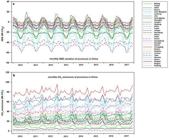
Figure 1.
The variations of monthly net ecosystem CO2 exchanges (a) and monthly CO2 emissions (b) in Mt CO2 for 31 provinces in China for the period of 2010–2017.
Analysis of the Multi-resolution Emission Inventory for China (MEIC) data revealed that CO2 emissions across all provinces displayed periodic variations, with higher emissions occurring primarily during the winter season (Figure 1b and Figure A3b). Among the provinces, Shandong, Jiangsu, and Hebei consistently ranked as the top three emitters of CO2. The periodic fluctuations in both net ecosystem CO2 exchange (NEE) and CO2 emissions resulted in corresponding variations in regional CO2 budgets for each province (Figure 2). Specifically, Shandong, Jiangsu, and Hebei had the highest positive CO2 budgets (80.47, 60.43, and 59.60 Mt CO2 per month, respectively), while Tibet, Yunnan, and Qinghai had the highest negative CO2 budgets (−48.28, −21.73, and −19.66 Mt CO2 per month, respectively) (Figure 2a and Figure A3c). When examining CO2 budget density, Shanghai exhibited significantly higher CO2 budget levels (2515.08 t CO2 km−2 per month) compared with other provinces, followed by Tianjin (1155.57 t CO2 km−2 per month) (Figure 2b and Figure A3d). As most provinces demonstrated positive CO2 budgets, atmospheric CO2 concentrations displayed an increasing trend with periodic variations each year (Figure 3 and Figure A3e). Notably, provinces such as Tibet, Yunnan, and Qinghai, which exhibited negative CO2 budgets, generally displayed lower atmospheric CO2 concentrations. However, these provinces still showed an upward trend in atmospheric CO2 levels over time. This observation suggests that the long-term effects of atmospheric CO2 cycling can contribute to the homogenization of CO2 concentrations, thereby influencing the heterogeneity of regional atmospheric CO2 sensitivity to regional CO2 budgets.
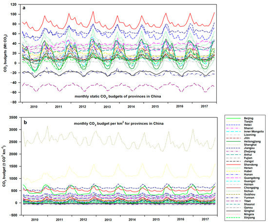
Figure 2.
The variations in monthly CO2 budget in Mt CO2 (a) and monthly CO2 budget density in t CO2 km−2 (b) for 31 provinces in China for the period of 2010–2017.
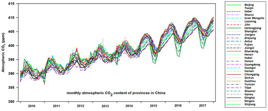
Figure 3.
The variations in monthly atmospheric CO2 contents in ppm for 31 provinces in China for the period of 2010–2017.
3.2. Regional Terrestrial NEE, CO2 Emissions, and Atmospheric CO2 Content
Pearson correlation analysis was conducted to examine the relationship between regional CO2 budgets and changes in regional atmospheric CO2 concentrations for various time intervals, ranging from monthly to twelve months, during the period of 2010–2017. It was anticipated that positive CO2 budgets would correspond to an increase in atmospheric CO2 concentrations. As such, the Pearson correlation coefficients were predominantly positive across most provinces, with the exception of Guangdong (Figure 4). Over time, a similar trend emerged among the provinces, with the Pearson coefficients initially increasing with longer time intervals and subsequently decreasing. Generally, the highest Pearson coefficients were observed with a six-month interval. However, in the coastal provinces of Fujian, Shanghai, Hainan, and Guangdong, weak correlations were found between changes in atmospheric CO2 concentrations and CO2 budgets, with corresponding Pearson coefficients of 0.242, 0.275, 0.117, and −0.268, respectively, for the six-month interval. It is worth noting that these four provinces are all coastal regions. Additionally, the coastal provinces of Zhejiang and Jiangsu exhibited relatively lower Pearson coefficients for the six-month interval (0.543 and 0.539, respectively) compared with the other provinces, which ranged between 0.60 and 0.80. These findings suggest that the interactions between CO2 budgets and CO2 transportation in coastal areas may influence atmospheric CO2 dynamics. In the short term, atmospheric CO2 transportation can disperse emitted CO2 and increase atmospheric CO2 concentrations. However, over a longer time frame, atmospheric CO2 transportation tends to homogenize regional atmospheric CO2 concentrations with those of other regions, thereby mitigating the impact of CO2 budgets on atmospheric CO2 levels.
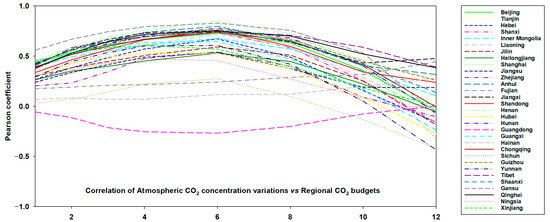
Figure 4.
The Pearson coefficient evolution of the correlation between regional atmospheric CO2 variations and regional CO2 budgets of 31 provinces in China for different periods of one month, two months, four months, six months, eight months, ten months, and twelve months.
While CO2 budgets played a significant role in explaining the variations in regional atmospheric CO2 concentrations, they alone were insufficient to fully account for these variations. Analysis of the collected data revealed that the atmospheric CO2 variations across all provinces did not exceed 10 ppm over a six-month period. However, the CO2 budgets for the same period in the 31 provinces resulted in atmospheric CO2 variations ranging from −17.32 ppm (Yunnan) to 768.12 ppm (Shanghai), with an average value of 78.24 ppm. These values take into consideration the accumulation of most CO2 within the troposphere, at altitudes ranging from 10 to 16 km, in China. Consequently, it is evident that other factors contribute significantly to the observed atmospheric CO2 variations.
Numerous studies have investigated the factors influencing regional atmospheric CO2 concentrations. For instance, Zhou et al. (2022) [19] identified monthly mean daily maximum global radiation, monthly effective accumulated temperature, monthly mean daily maximum vapor pressure deficit, and monthly precipitation as the key meteorological variables influencing atmospheric CO2 in forest systems. Yang et al. (2020) [20] found that soil temperature, air temperature, photosynthetically active radiation (PAR), below-canopy CO2 concentration, vapor pressure deficit, and soil water content at 50 cm were the main meteorological factors influencing CO2 exchange on daily and monthly time scales. Other meteorological factors, such as wind patterns, can also play a crucial role in atmospheric CO2 dynamics by affecting its transport [21,22]. Although multiple factors can influence atmospheric CO2, they can be broadly categorized as CO2 budgets and CO2 transport within the atmosphere.
In the previous section, we developed an NEE estimation model that incorporated potential factors affecting atmospheric CO2, such as surface temperature, soil temperature, surface net solar radiation, precipitation, evaporation, soil water content, NDVI index, EVI index, canopy height, and forest age, to calculate CO2 budgets. To explore the interactive effects of CO2 budgets and CO2 transport, including winds, surface turbulence stress, forecast surface roughness, convective available potential energy, boundary layer height, boundary layer dissipation, and sub-grid scale orography, on atmospheric CO2 variations over a six-month period, a redundancy analysis (RDA) was conducted.
RDA biplots were generated to illustrate the contributions of the considered factors to the variations in atmospheric CO2 (deltaCO2) and atmospheric CO2 content (CO2). The projection of each factor’s arrow onto the arrow of the focused variables indicated the direction and intensity of its effect. For example, Figure 5 depicts that, in the case of Beijing, the factors of budgetCO2, w10, w100, mtss, bld, and fsr all positively contributed to deltaCO2, while only parameters blh and cape had negative contributions. Conversely, in Tianjin, only budgetCO2 had a positive contribution to deltaCO2, while the other factors had negative contributions. Furthermore, for both Beijing and Tianjin, the considered factors appeared to have minimal effects on atmospheric CO2 content (CO2) since their arrows were nearly orthogonal to the CO2 arrow. RDA biplots for the other 29 provinces can be found in Figure A4. The RDA results indicated that CO2 budgets and climatic transport parameters directly influenced the variation in atmospheric CO2 (deltaCO2), but not atmospheric CO2 content (CO2) (Figure A3). In most cases, deltaCO2 showed a strong positive correlation with CO2 budgets, except for the coastal provinces of Shanghai, Fujian, Guangdong, and Hainan, which aligned with the results of the correlation analysis. Additionally, deltaCO2 tended to be predominantly influenced by parameters such as fsr (21/31 provinces), blh (26/31 provinces), and cape (31/31 provinces), resulting in negative effects. The boundary layer, where emitted pollutants mix [23,24], is likely to have a similar effect on emitted CO2. Thus, a higher boundary layer favors the diffusion of emitted CO2 to the free atmospheric layer, reducing local CO2 accumulation. Similarly, convective available potential energy (cape), which represents the integrated work that positive buoyancy forces would perform on air parcels rising vertically through the atmosphere, inhibits the uplift of pollutants when it is negative [25]. Consequently, higher cape values contributed to the atmospheric diffusion of emitted CO2. In comparison to other parameters, mtss and bld had relatively less impact on deltaCO2.
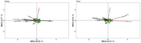
Figure 5.
The redundancy analysis biplots of factor scores for average atmospheric CO2 contents (CO2) and atmospheric CO2 variations (deltaCO2) for every six months during the period of 2010–2017 for the regions of Beijing and Tianjin. The considered factors included CO2 budget (budgetCO2), average wind strength at 100 m and 10 m heights (w100 and w10), average mean turbulence surface stress (mtss), forecast surface roughness (fsr), convective available potential energy (cape), boundary layer height and dissipation (blh and bld), and angle of sub-grid scale orography (anor).
Furthermore, the parameters of boundary layer height (blh) and convective available potential energy (cape) primarily affected the vertical movements of atmospheric CO2, whereas its horizontal movement was driven by winds. The RDA analysis also revealed that wind strength at 100 m and 10 m heights (w100 and w10) were significant factors influencing deltaCO2. However, their relationship with deltaCO2 varied, with both positive and negative associations observed.
For the provinces of Tianjin, Liaoning, Shanghai, Jiangsu, Shandong, Henan, Guizhou, Shaanxi, and Xinjiang, w100 and w10 exerted a negative influence on deltaCO2. As w100 and w10 represent cumulative winds for each province, this suggests that winds tend to transport CO2 out of these provinces. It is important to note that this is not necessarily due to higher atmospheric CO2 contents in these provinces (Figure A5a), but rather their CO2 budgets. Some of these provinces exhibited the highest annual CO2 budgets in China, such as Shanghai, Tianjin, Jiangsu, and Shandong, with values of 20,120.66, 9244.60, 5023.94, and 4185.66 t CO2 km−2, respectively, ranking among the top four provinces (calculated from Figure 2b). Additionally, other provinces showed significantly higher annual CO2 budgets compared with their neighboring provinces, such as Liaoning and Henan (Figure A5b). These findings indicate that the atmospheric CO2 variations in a particular province are influenced not only by its own CO2 budget but also by the budgets of other provinces.
Geographically weighted regression results demonstrated a weak linear relationship between regional atmospheric CO2 variations and their own CO2 budgets over a six-month period, as indicated by several negative slope factors (Figure 6a) and R2 values below 0.4 (Figure 6b).
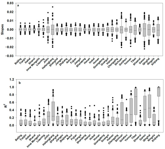
Figure 6.
The box-plots of estimated slopes (a) and determination coefficients (R2) (b) of the geographically weighted regression of regional atmospheric CO2 variations and regional CO2 budgets for 31 provinces. The whiskers, upper and lower edge of boxes, and horizontal line inside boxes represent, from bottom to top, the minimum, first quartile, median, third quartile, and maximum of the values calculated for every six-month interval, while the black points represent the outliers.
In summary, the contents of atmospheric CO2 were influenced by a combination of CO2 budgets and atmospheric transportation. While our findings indicate that regional CO2 budgets alone may not fully account for the variations observed in regional atmospheric CO2, they still exert significant impacts and demonstrate meaningful positive correlations with atmospheric CO2 variations over a relatively short-term period of six months.
3.3. Emission Allocation Policies Related to CO2 Budgets
Unlike the findings of previous studies, such as Zhang et al. (2022) [14], which suggested that changes in CO2 source and sink characteristics played a joint role in decreasing atmospheric CO2 concentration over a three-year period in the Nanling area of China, our results indicate that regional CO2 budgets alone do not exert dominant influence on altering regional atmospheric CO2 at the provincial scale. One possible explanation for this disparity could be the presence of point sources emitting CO2, whereby the increase in atmospheric CO2 resulting from positive CO2 budgets might be more pronounced in specific localized areas within each province. Therefore, it may be necessary to analyze the relationship between CO2 budgets and atmospheric CO2 at a smaller scale, focusing on sub-regions or localized areas. To support this notion, we conducted a similar correlation analysis by aggregating data from provinces into larger regions of China, namely northeast China, north China, central China, south China, east China, southwest China, and northwest China. The results revealed that the correlation between CO2 budgets and changes in atmospheric CO2 content weakened at the regional and national scales compared with the provincial level (Figure A6). Consequently, regional CO2 budgets may have a more significant impact on atmospheric CO2 dynamics in smaller areas, contributing to both positive and negative effects on specific microcosms such as temperature increase [26], growth pressure on vegetation [27], and CO2 fertilization effects [28].
Furthermore, the regional sensitivity of atmospheric CO2 to CO2 budgets can lead to an imbalanced distribution of atmospheric CO2 and variations in warming patterns. This imbalance can potentially lead to overestimation or underestimation of the costs associated with warming in specific areas, making it challenging to develop comprehensive carbon emission allocation policies that ensure fairness and efficiency. In our view, an optimized emission allocation strategy should aim to achieve a balance between carbon emissions and uptake in each region, such as provinces or even cities, to establish an acceptable CO2 budget. This approach would enable effective control of regional atmospheric CO2 variations and minimize potential damages to regional ecosystems. To implement such a carbon allocation strategy, detailed information on regional emissions, the CO2 uptake capacity of ecosystems, and CO2 transport flux needs to be obtained. Numerous efforts have already been made to estimate gridded CO2 emissions [29,30], carbon budgets of terrestrial ecosystems [31,32], CO2 diffusion flux [33], as well as advancements in techniques for processing remote sensing air data [34,35]. Encouraging further research in these areas is crucial for gaining a comprehensive understanding of regional carbon dynamics.
4. Conclusions
This study demonstrates that CO2 budgets have a considerable influence, though not a dominant one, on the alteration of atmospheric CO2 over a six-month period in most provinces of China. Moreover, the findings highlight the potential effects of different regional CO2 budgets on the uneven distribution of atmospheric CO2, particularly at smaller scales below the provincial level. Therefore, it is essential not to overlook these effects and instead promote further monitoring research on gridded CO2 emissions and uptake, as well as studies focusing on regional CO2 variations and their impact on local ecosystem functions. These endeavors will contribute to the development of a more comprehensive CO2 emission allocation strategy that takes into account both economic and ecological factors related to CO2 generation and uptake. By doing so, potential ecological risks can be mitigated, ensuring a balanced approach to carbon management.
Author Contributions
H.L. and Y.L.—Software, Formal analysis, Methodology, Writing—Original Draft, Visualization, Funding acquisition; Q.R. and L.L.—Conceptualization, Methodology, Visualization, Supervision, Writing—Review and Editing, Funding acquisition; Z.Q. and L.-C.L.—Data Curation, Formal analysis, Methodology, Writing—Review and Editing. All authors have read and agreed to the published version of the manuscript.
Funding
This study was funded by the National Basic Survey Project (2019FY202501-03), the Foundation of Tianjin Normal University (52XB1502, 043-135202XK1604), and the National Natural Science Foundation of China (Grant No. 41971306).
Data Availability Statement
Publicly available datasets were analyzed in this study. These data can be found here: https://ameriflux.lbl.gov/; https://fluxnet.org/; https://cds.climate.copernicus.eu/; https://glad.umd.edu/dataset/global-2010-tree-cover-30-m; https://doi.pangaea.de/10.1594/PANGAEA.889943; http://meicmodel.org.cn/; https://disc.gsfc.nasa.gov/datasets/AIRS3C2M_005/summary, all accessed on 1 December 2022.
Acknowledgments
We thank Noura Ziadi and Yichao Shi for giving us some ideas on this topic and the ways to access the necessary data.
Conflicts of Interest
The authors declare no conflict of interest.
Appendix A

Figure A1.
Flowchart of data collection, model construction, and data analyses.

Figure A2.
Scatter plots of calculated versus observed NEE values for the testing dataset.

Figure A3.
Box-plots of monthly net ecosystem CO2 exchanges (a), monthly CO2 emissions (b), monthly CO2 budgets (c), monthly CO2 budget densities (d), and monthly atmospheric CO2 contents (e) for 31 provinces in China for the period of 2010–2017.

Figure A4.
The redundancy analysis biplots of factor scores for average atmospheric CO2 contents (CO2) and atmospheric CO2 variations (deltaCO2) for every six months during the period of 2010–2017. The considered factors included CO2 budget (budgetCO2), average wind strength at 100m and 10m heights (w100 and w10), average mean turbulence surface stress (mtss), forecast surface roughness (fsr), convective available potential energy (cape), boundary layer height and dissipation (blh and bld), and angle of sub-grid scale orography (anor). If the province had w100 and w10 contributing positively to deltaCO2, it indicated atmospheric CO2 was transported into the province. On the contrary, atmospheric CO2 was transported out from the province.

Figure A5.
The distribution of average monthly atmospheric CO2 contents (a) and average monthly CO2 budget densities (b) for 31 provinces in China.

Figure A6.
The Pearson coefficient evolution of the correlation between regional atmospheric CO2 variations and regional CO2 budgets of 7 grand regions in China and the whole country for different periods of one month, two months, four months, six months, eight months, ten months, and twelve months.
References
- Dong, L.; Miao, G.; Wen, W. China’s Carbon Neutrality Policy: Objectives, Impacts and Paths. East Asian Policy 2021, 13, 5–18. [Google Scholar] [CrossRef]
- Jiang, H.; Shao, X.; Zhang, X.; Bao, J. A Study of the Allocation of Carbon Emission Permits among the Provinces of China Based on Fairness and Efficiency. Sustainability 2017, 9, 2122. [Google Scholar] [CrossRef]
- Fang, G.; Liu, M.; Tian, L.; Fu, M.; Zhang, Y. Optimization Analysis of Carbon Emission Rights Allocation Based on Energy Justice—The Case of China. J. Clean. Prod. 2018, 202, 748–758. [Google Scholar] [CrossRef]
- Zhou, H.; Ping, W.; Wang, Y.; Wang, Y.; Liu, K. China’s Initial Allocation of Interprovincial Carbon Emission Rights Considering Historical Carbon Transfers: Program Design and Efficiency Evaluation. Ecol. Indic. 2021, 121, 106918. [Google Scholar] [CrossRef]
- Sim, J. A Carbon Emission Evaluation Model for a Container Terminal. J. Clean. Prod. 2018, 186, 526–533. [Google Scholar] [CrossRef]
- Baldocchi, D.; Penuelas, J. The Physics and Ecology of Mining Carbon Dioxide from the Atmosphere by Ecosystems. Glob. Chang. Biol. 2019, 25, 1191–1197. [Google Scholar] [CrossRef]
- Sengupta, S.; Gorain, P.C.; Pal, R. Aspects and Prospects of Algal Carbon Capture and Sequestration in Ecosystems: A Review. Chem. Ecol. 2017, 33, 695–707. [Google Scholar] [CrossRef]
- Rivela, C.B.; Blanco, M.B.; Teruel, M.A. Atmospheric Degradation of Industrial Fluorinated Acrylates and Methacrylates with Cl Atoms at Atmospheric Pressure and 298 K. Atmos. Environ. 2018, 178, 206–213. [Google Scholar] [CrossRef]
- Yang, Y.; Liu, L.; Zhang, F.; Zhang, X.; Xu, W.; Liu, X.; Wang, Z.; Xie, Y. Soil Nitrous Oxide Emissions by Atmospheric Nitrogen Deposition over Global Agricultural Systems. Environ. Sci. Technol. 2021, 55, 4420–4429. [Google Scholar] [CrossRef]
- Wuebbles, D.J.; Hayhoe, K. Atmospheric Methane and Global Change. Earth Sci. Rev. 2002, 57, 177–210. [Google Scholar] [CrossRef]
- Nakazawa, T. Current Understanding of the Global Cycling of Carbon Dioxide, Methane, and Nitrous Oxide. Proc. Jpn. Acad. Ser. B 2020, 96, 394–419. [Google Scholar] [CrossRef] [PubMed]
- Siljanen, H.M.P.; Welti, N.; Voigt, C.; Heiskanen, J.; Biasi, C.; Martikainen, P.J. Atmospheric Impact of Nitrous Oxide Uptake by Boreal Forest Soils Can Be Comparable to That of Methane Uptake. Plant Soil 2020, 454, 121–138. [Google Scholar] [CrossRef]
- Fu, C.; Dan, L.; Feng, J.; Peng, J.; Yin, N. Temporal and Spatial Heterogeneous Distribution of Tropospheric CO2 over China and Its Possible Genesis. Chin. J. Geophys. 2018, 61, 4373–4382. [Google Scholar] [CrossRef]
- Zhang, C.; Wu, G.; Wang, H.; Wang, Y.; Gong, D.; Wang, B. Regional Effect as a Probe of Atmospheric Carbon Dioxide Reduction in Southern China. J. Clean. Prod. 2022, 340, 130713. [Google Scholar] [CrossRef]
- Lian, Y.; Li, H.; Renyang, Q.; Liu, L.; Dong, J.; Liu, X.; Qu, Z.; Lee, L.-C.; Chen, L.; Wang, D.; et al. Mapping the Net Ecosystem Exchange of CO2 of Global Terrestrial Systems. Int. J. Appl. Earth Obs. Geoinf. 2023, 116, 103176. [Google Scholar] [CrossRef]
- Oksanen, J.; Kindt, R.; Legendre, P.; O’Hara, B.; Stevens, M.H.H.; Oksanen, M.J.; Suggests, M. The Vegan Package. Community Ecol. Package 2007, 10, 719. [Google Scholar]
- Fotheringham, A.S.; Brunsdon, C.; Charlton, M. Geographically Weighted Regression: The Analysis of Spatially Varying Relationships; John Wiley & Sons: Hoboken, NJ, USA, 2003. [Google Scholar]
- Huang, N.; Wang, L.; Zhang, Y.; Gao, S.; Niu, Z. Estimating the Net Ecosystem Exchange at Global FLUXNET Sites Using a Random Forest Model. IEEE J. Sel. Top. Appl. Earth Obs. Remote Sens. 2021, 14, 9826–9836. [Google Scholar] [CrossRef]
- Zhou, Y.; Zhang, J.; Yin, C.; Huang, H.; Sun, S.; Meng, P. Empirical Analysis of the Influences of Meteorological Factors on the Interannual Variations in Carbon Fluxes of a Quercus Variabilis Plantation. Agric. For. Meteorol. 2022, 326, 109190. [Google Scholar] [CrossRef]
- Yang, J.; Duan, Y.; Yang, X.; Awasthi, M.K.; Li, H.; Zhang, L. Modeling CO2 Exchange and Meteorological Factors of an Apple Orchard Using Partial Least Square Regression. Environ. Sci. Pollut. Res. 2020, 27, 43439–43451. [Google Scholar] [CrossRef]
- Hernández-Paniagua, I.Y.; Lowry, D.; Clemitshaw, K.C.; Fisher, R.E.; France, J.L.; Lanoisellé, M.; Ramonet, M.; Nisbet, E.G. Diurnal, Seasonal, and Annual Trends in Atmospheric CO2 at Southwest London during 2000–2012: Wind Sector Analysis and Comparison with Mace Head, Ireland. Atmos. Environ. 2015, 105, 138–147. [Google Scholar] [CrossRef]
- Lauderdale, J.M.; Garabato, A.C.N.; Oliver, K.I.C.; Follows, M.J.; Williams, R.G. Wind-Driven Changes in Southern Ocean Residual Circulation, Ocean Carbon Reservoirs and Atmospheric CO2. Clim. Dyn. 2013, 41, 2145–2164. [Google Scholar] [CrossRef]
- Jia, W.; Zhang, X. The Role of the Planetary Boundary Layer Parameterization Schemes on the Meteorological and Aerosol Pollution Simulations: A Review. Atmos. Res. 2020, 239, 104890. [Google Scholar] [CrossRef]
- Lee, J.; Hong, J.-W.; Lee, K.; Hong, J.; Velasco, E.; Lim, Y.J.; Lee, J.B.; Nam, K.; Park, J. Ceilometer Monitoring of Boundary-Layer Height and Its Application in Evaluating the Dilution Effect on Air Pollution. Bound. Layer Meteorol. 2019, 172, 435–455. [Google Scholar] [CrossRef]
- Wang, J.; Yang, Y.; Zhang, X.; Liu, H.; Che, H.; Shen, X.; Wang, Y. On the Influence of Atmospheric Super-Saturation Layer on China’s Heavy Haze-Fog Events. Atmos. Environ. 2017, 171, 261–271. [Google Scholar] [CrossRef]
- Lee, J.Y.; Kim, H.; Gasparrini, A.; Armstrong, B.; Bell, M.L.; Sera, F.; Lavigne, E.; Abrutzky, R.; Tong, S.; Coelho, M.d.S.Z.S.; et al. Predicted Temperature-Increase-Induced Global Health Burden and Its Regional Variability. Environ. Int. 2019, 131, 105027. [Google Scholar] [CrossRef]
- Lammertsma, E.I.; de Boer, H.J.; Dekker, S.C.; Dilcher, D.L.; Lotter, A.F.; Wagner-Cremer, F. Global CO2 Rise Leads to Reduced Maximum Stomatal Conductance in Florida Vegetation. Proc. Natl. Acad. Sci. USA 2011, 108, 4035–4040. [Google Scholar] [CrossRef]
- Fernández-Martínez, M.; Sardans, J.; Chevallier, F.; Ciais, P.; Obersteiner, M.; Vicca, S.; Canadell, J.G.; Bastos, A.; Friedlingstein, P.; Sitch, S.; et al. Global Trends in Carbon Sinks and Their Relationships with CO2 and Temperature. Nat. Clim. Chang. 2019, 9, 73–79. [Google Scholar] [CrossRef]
- Zhang, Y.; Liu, X.; Lei, L.; Liu, L. Estimating Global Anthropogenic CO2 Gridded Emissions Using a Data-Driven Stacked Random Forest Regression Model. Remote Sens. 2022, 14, 3899. [Google Scholar] [CrossRef]
- Wang, J.; Cai, B.; Zhang, L.; Cao, D.; Liu, L.; Zhou, Y.; Zhang, Z.; Xue, W. High Resolution Carbon Dioxide Emission Gridded Data for China Derived from Point Sources. Environ. Sci. Technol. 2014, 48, 7085–7093. [Google Scholar] [CrossRef]
- Chen, B.; Zhang, H.; Wang, T.; Zhang, X. An Atmospheric Perspective on the Carbon Budgets of Terrestrial Ecosystems in China: Progress and Challenges. Sci. Bull. 2021, 66, 1713–1718. [Google Scholar] [CrossRef]
- Wang, J.; Feng, L.; Palmer, P.I.; Liu, Y.; Fang, S.; Bösch, H.; O’Dell, C.W.; Tang, X.; Yang, D.; Liu, L.; et al. Large Chinese Land Carbon Sink Estimated from Atmospheric Carbon Dioxide Data. Nature 2020, 586, 720–723. [Google Scholar] [CrossRef] [PubMed]
- Wang, F.; Cao, M.; Wang, B.; Fu, J.; Luo, W.; Ma, J. Seasonal Variation of CO2 Diffusion Flux from a Large Subtropical Reservoir in East China. Atmos. Environ. 2015, 103, 129–137. [Google Scholar] [CrossRef]
- Semlali, B.-E.B.; Amrani, C.E. A Stream Processing Software for Air Quality Satellite Datasets. In Advanced Intelligent Systems for Sustainable Development (AI2SD’2020); Kacprzyk, J., Balas, V.E., Ezziyyani, M., Eds.; Springer International Publishing: Cham, Switzerland, 2022; pp. 839–853. [Google Scholar]
- Semlali, B.-E.B.; Amrani, C.E.; Ortiz, G.; Boubeta-Puig, J.; Garcia-de-Prado, A. SAT-CEP-Monitor: An Air Quality Monitoring Software Architecture Combining Complex Event Processing with Satellite Remote Sensing. Comput. Electr. Eng. 2021, 93, 107257. [Google Scholar] [CrossRef]
Disclaimer/Publisher’s Note: The statements, opinions and data contained in all publications are solely those of the individual author(s) and contributor(s) and not of MDPI and/or the editor(s). MDPI and/or the editor(s) disclaim responsibility for any injury to people or property resulting from any ideas, methods, instructions or products referred to in the content. |
© 2023 by the authors. Licensee MDPI, Basel, Switzerland. This article is an open access article distributed under the terms and conditions of the Creative Commons Attribution (CC BY) license (https://creativecommons.org/licenses/by/4.0/).