Unlocking the Potential of Remote Sensing in Wind Erosion Studies: A Review and Outlook for Future Directions

Abstract

Remote sensing (RS) has revolutionized field data collection processes and provided timely and spatially consistent acquisition of data on the terrestrial landscape properties. This research paper investigates the relationship between Wind Erosion (WE) and Remote Sensing (RS) techniques. By examining, analyzing, and reviewing recent studies utilizing RS, we underscore the importance of wind erosion research by exploring indicators that influence the detection, evaluation, and modeling of wind erosion. Furthermore, it identifies research gaps particularly in soil erodibility estimation, soil moisture monitoring, and surface roughness assessment using RS. Overall, this research enhances our understanding of WE and RS and offers insights into future research directions. To conduct this study, we employed a two-fold approach. First, we utilized a non-systematic review approach by accessing the Global Applications of Soil Erosion Modelling Tracker (GASEMT) database. Subsequently, we conducted a systematic review of the relevant literature on wind erosion and remote sensing in the core collection of the Web of Science (WoS) database. Additionally, we employed the VOSviewer bibliometric software to generate a cooperative keyword network analysis, facilitating the advancements and identifying emerging areas of WE and RS research. With a non-systematic review, we focused on examining the current state and potential of remote sensing for mapping and analyzing following indicators of wind erosion modelling: (1) soil erodibility; (2) soil moisture; (3) surface roughness; (4) vegetation cover; (5) wind barriers; and (6) wind erosion mapping. Our study highlights the widespread utilization of freely available RS data, such as MODIS and Landsat, for WE modeling. However, we also acknowledge the limitations of high resolution sensors due to their high costs. RS techniques offer an efficient and cost-effective approach for mapping erosion at various scales and call for a more comprehensive and detailed assessment of soil erosion at regional scales. These findings provide valuable guidance for future research endeavors in this domain.

1. Introduction

Wind erosion is a natural soil degradation process [1], often accelerated by human activity [2]. The erosion events caused by wind lead to the depletion of fine particles such as clay and silt [3] and organic matter [4], which can result in decreased soil productivity and degradation of the soil’s hydrothermal properties [5]. Wind erosion (WE) predominantly occurs in regions characterized by low precipitation and high evaporation rates, which cover roughly one-third of the global land area and 12% of Europe [6]. Climate change has intensified WE in semi-arid areas by 3.2% from 1980 to 2019 [7]. The United Nations (UN) global soil resources report highlights that a significant proportion of the world’s soil is in suboptimal conditions [8]. Soil erosion, loss of soil carbon, and nutrient imbalance pose significant threats to soil functions.

The process of WE has three phases: (1) initiation of the movement of the soil particles (detachment or deflation), (2) the transportation of the soil particles (suspension, saltation, and surface creep), and (3) the deposition [9,10]. Several models have been developed to simulate the WE [11,12] and estimate the erosion intensity and effectiveness of erosion control strategies [13]. Empirical models are based on observed data and their statistical relationship with analyzed predictors. This approach is simpler, criticized for employing unrealistic assumptions, ignoring heterogeneity of inputs and nonlinear relationships between input parameters [14]. Most empirical models compute soil loss and do not simulate transportation or deposition [11]. Physical models, or process-based models, are based on understanding of the whole process of aeolian transport [15]. The distinction between the models is not always clear, and both approaches could be integrated into one model [2]. Some of the main challenges in aeolian transport modeling have been as identified the fidelity of process representation, up-scaling the presence of heterogeneity, spatial data availability, and large-scale parameter estimation [15].

The management of WE presents a formidable challenge because it involves intricate interplay due to complex interactions among driving forces, pressures, and ecosystem states [16]. Due to the intricate nature of the process, it remains challenging to oversee and measure soil WE on a larger scale [17]. The study of WE involves a range of research techniques, such as laboratory and field measurements, modelling, and the use of remote sensing (RS) technologies. While methods such as wind tunnel testing and direct terrain measurements are commonly employed, they are often constrained by time and environmental factors, and may not fully capture the complex and dynamic spatial and temporal aspects of WE. However, the accuracy of these methods is still being improved [11,18]. In the last two decades, RS [19] and computer technology have made significant progress, with increased technological potential to obtain more relevant data on WE [17]. RS methods are faster than ground methods, can cover large areas, and facilitate repeated monitoring of erosion events or factors affecting the erosion [18,20,21,22]. The employment of RS technology provides the opportunity to efficiently evaluate soil quality at different scales, with the added benefits of speed and affordability. Nevertheless, the variation in the spectral response of soils at different depths and the disparities in the spatial, spectral, and temporal resolutions of various sensors could necessitate extensive data processing and intricate models [23]. Satellite imagery allows for the quick and timely recording of the presence and intensity of erosion processes, the prediction of their impact on the topography, soils, agricultural land, and landscape systems, and approval of a set of measures to reduce the negative effects on the natural surroundings [24]. The European Space Agency’s (ESA) release of the Sentinel 2 sensor, which boasts an average spatial resolution of 10 m and a 5-day revisiting cycle, has made it one of the most widely accessible and practical sources of remote sensing data for soil erosion mapping and modeling, second only to the Landsat series [21]. The new RS systems, including drones and LiDAR, produce the data in higher spatial, temporal, and spectral resolution [18,25]. Additionally, the increasing computer power enables the large-scale application of some detailed approaches used in local scales. Incorporating RS data into WE modeling is anticipated to enhance the accuracy and decrease the level of ambiguity or imprecision present in the model [25,26].

The potential to integrate RS, spatial analysis, geographic information system (GIS), and modelling into WE analyses is still a great challenge. Previous reviews were focused on using RS in erosion or land degradation mapping in general [18,20,22], or were directly focused on WE models [11,12], or the representation of aeolian processes [2,15]. This manuscript reviews the RS approaches used to derive the input parameters for WE models and we analyze the potential of advanced RS methods for improving the quality of main input parameters for WE models.

2. Materials and Methods

To gain a comprehensive understanding of the application of remote sensing (RS) in wind erosion (WE) assessment, we combined a non-systematic and systematic review approach. To conduct the systematic review, the Web of Science (WoS) core collection database was searched for relevant literature on WE and remote sensing. For the non-systematic review, the ‘Global Applications of Soil Erosion Modelling Tracker (GASEMT)’ database was utilized. This database includes studies published between 1994 and 2018 and is publicly available to users [27]. This review expanded the analysis of the GASEMT database by examining the connection between soil erosion modelling and RS. In this review paper, the impact of six factors that are facilitated in WE studies with the help of RS was evaluated: soil erodibility, soil moisture, surface roughness, vegetation cover, wind barriers, and WE mapping. In each factor, the research and also the future perspectives were examined.

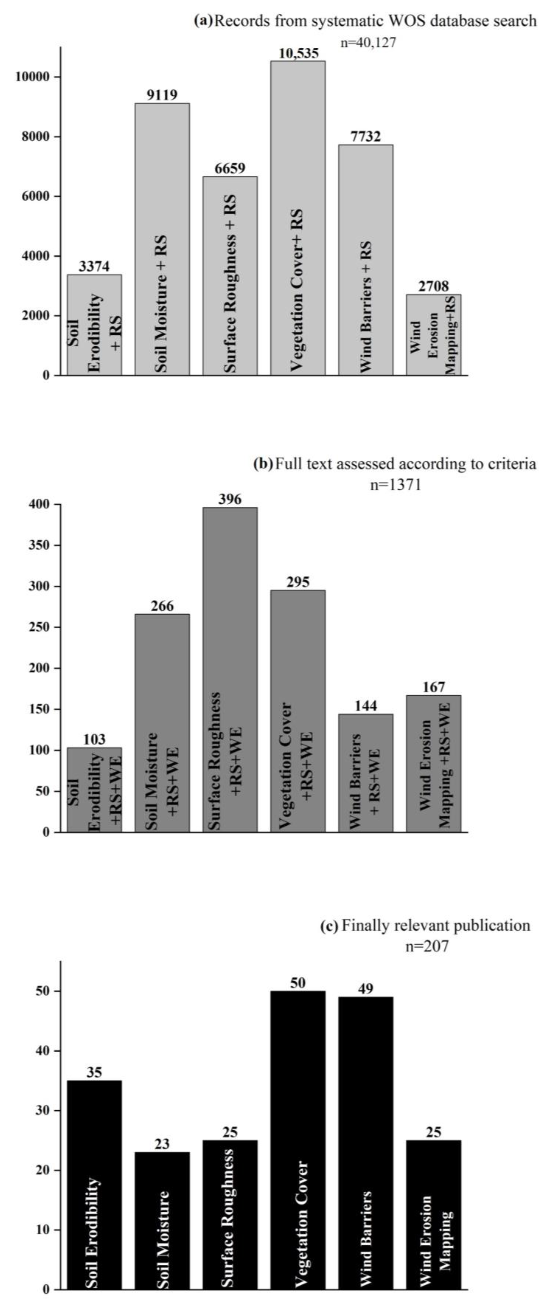
Systematic and Non-Systematic Literature Research

We conducted a bibliographic investigation in September–November 2022 in the WoS database. The query “wind erosion” + “remote sensing” generated 237 research papers, published between 1991 and 2022. We used VOSviewer bibliometric software version 1.6. to draw the cooperative network and keyword co-occurrence map to analyze the research progress and frontier [28].

We used a classical review approach based on non-systematic literature research in databases, SCOPUS, WoS, and Google Scholar. We used search terms such as “Wind erosion modelling, Wind erosion models, Wind erosion mapping, RS, Soil erodibility, Soil moisture, Surface roughness, Vegetation cover, Wind barriers, etc.” to obtain a set of papers focusing on wind erosion modelling and then we searched in the reference literature or used specific queries to obtain additional information.

We restricted our review to those model input parameters that are commonly used in WE models [11,12] and are derived or could be derived with use of RS. These WE models include basic parameters such as soil erodibility, soil moisture, soil roughness, vegetation cover, wind barriers, climate inputs, and other inputs such as threshold velocity, management, and so on. Soil erodibility is used in all the models and is derived from the percentage of sand soil particles and for some models forms additional soil physical parameters. Soil moisture is used directly as an input parameter or is estimated indirectly from the climate parameters. Surface roughness is included in models directly as specific input parameter or indirectly as tillage parameter or soil surface condition parameter. Vegetation or crop cover is directly included in most of the models or is covered in management or surface cover parameters. Wind barriers are related to field length, field geometry and wind speed. Additionally, we reviewed the application of RS methods for WE mapping because the RS is often used for verification of WE models, and in some cases the RS approach could be an alternative to WE models.

Figure 1 shows a flowchart with the results at the different stages of this study taken from the initial WoS search to the final selection of possible papers of interest for this review paper. Even though this was a specific and very stringent search, aimed at excluding unrelated articles from the beginning, the WoS output still generated a relatively large number of 40,127 publications for all six factors (a). As shown in Figure 1a, all the research conducted on the six investigated factors are included in the WoS database with the restriction of “remote sensing”. Following the evaluation of the papers according to the research interest, the cutting point for considering articles for further evaluation depended on the strong and effective relationship to the topic in this step. In this case, 1371 articles were considered for reading their full abstracts by the terms “Wind Erosion” as a restriction for all six evaluated factors (b). Finally, the relevant articles (n = 207) which emphasize the relationship of chosen factors with the terms “Wind Erosion” and “Remote Sensing” for more interdisciplinary research were investigated (c).

Although the climate parameters are crucial for WE modelling, we did not include them in our review, because they are commonly derived from meteorological data and models, and we do not see any potential for RS in this area. In the second phase, we estimated the current and future potential of RS for improving the quality of the input parameters for WE models.

3. Results

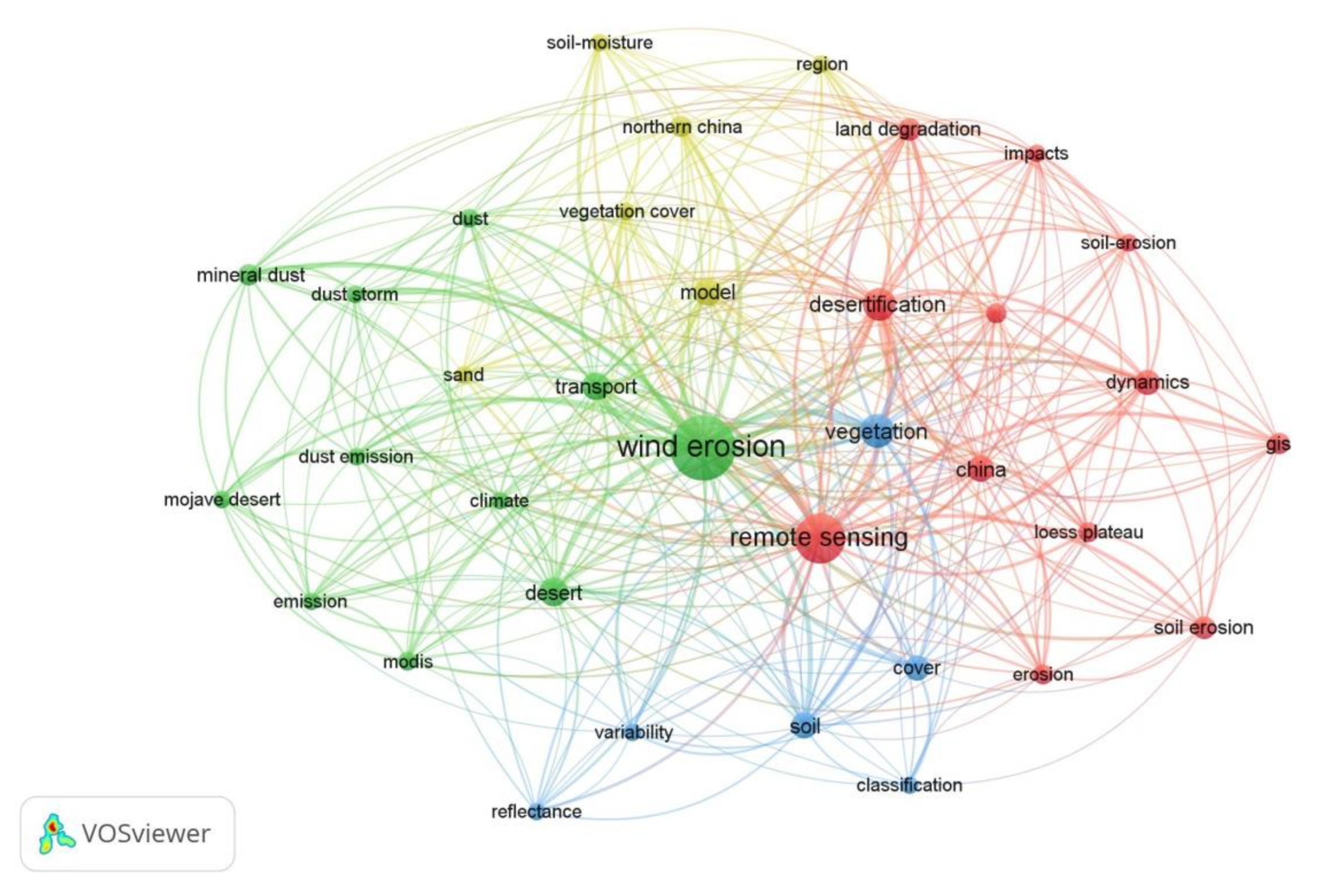
3.1. Research Frontiers

In Figure 2, the keyword network analysis map reveals the existence of four groups that represent distinct research areas related to WE and RS. Group 1 is mainly focused on utilizing RS techniques to evaluate land degradation and erosion. This is demonstrated by terms such as “erosion”, “land degradation”, “desertification”, and “impacts”. The terms “China” and “loess plateau” indicate an interest in the dominant interest in land degradation in these regions.

Groups are identified by color (Group 1—red; 2—green; 3—blue and 4—yellow). The size of the labels and circles in the figure is directly proportional to the frequency of occurrences. The lines connecting the terms indicate significant connections, with the thickness of the lines representing the strength of the association. Additionally, the distance between the terms in the figure also reflects the strength of the association.

The Group 2 research fronts are focused on the effect of WE on dust emission, as indicated by the link to terms “emission”, “dust”, and “desert” with terms of “modis” and “transport”. The time-series MODIS data are utilized for the purpose of identifying the erodibility of landscapes and mapping the hazard of WE during different seasons [29]. Group 3 pertains to the use of RS classification of vegetation cover as a crucial input for WE modeling. This is evident from the presence of terms such as “cover”, “variability”, “reflectance”, and “classification”. Group 3’s position on the network map suggests that it has a stronger association and greater connectivity with Group 1. On the other hand, Group 4 is focused on WE modeling and has a regional scope, as indicated by the frequent occurrence of terms such as “model” and “region”. The application of RS for analyzing the inputs such as “vegetation cover”, “soil moisture”, and “sand” for erosion models is visible here as well. The frequent use of the term “dust” and “desert” shows the increasing importance of desertification. The co-occurrence groups highlight two distinct trends:

-

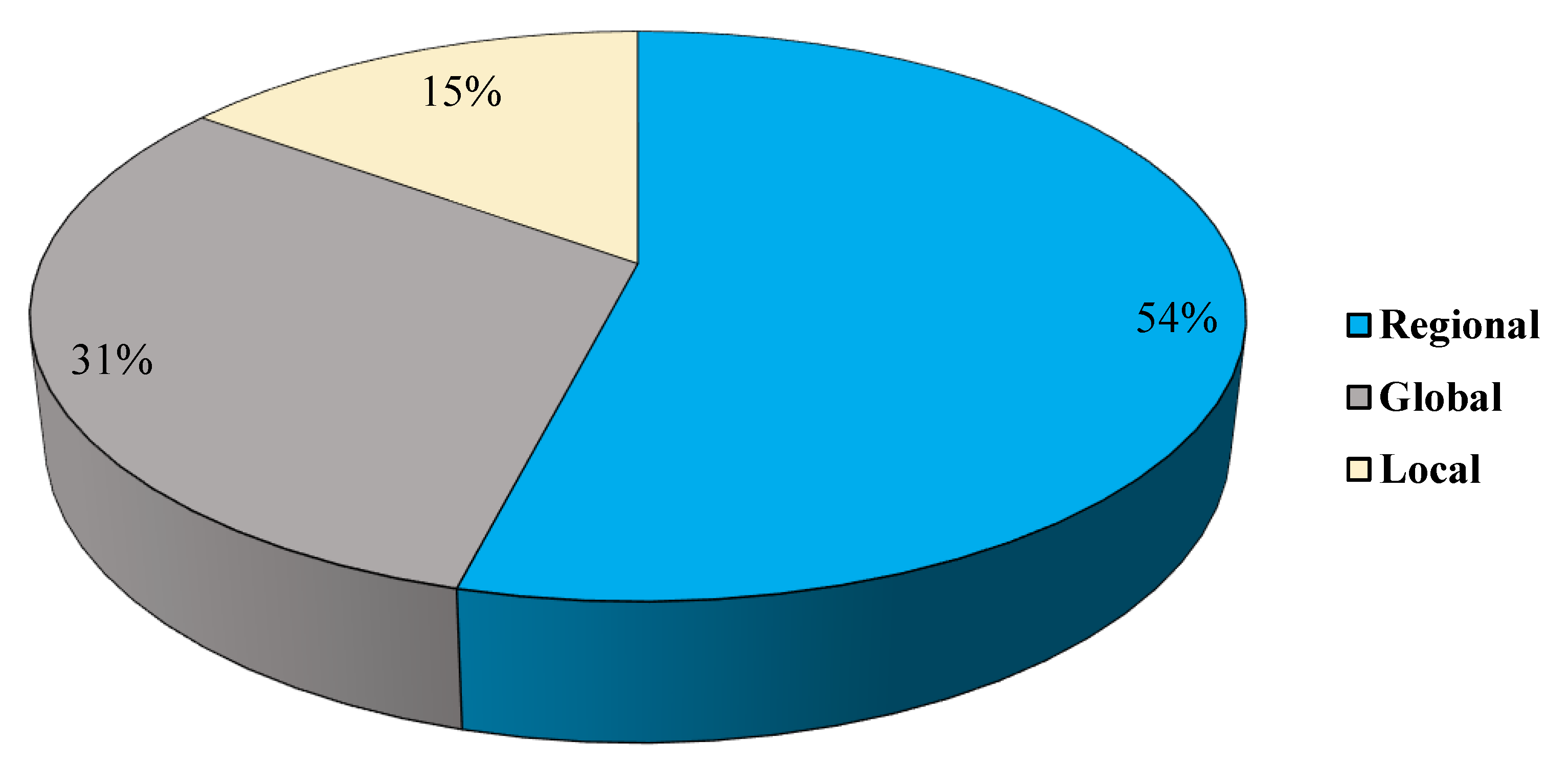
The majority of studies in the field of WE and RS are completed on a regional scale;

-

The research emphasizes more variable and effective factors in the process of erosion. The frequent use of terms such as “vegetation” and “climate change” shows this trend.

3.2. Remote Sensors and Indicators Used in Wind Erosion Modelling

Recent soil survey data, such as the LUCAS topsoil and RS data, have made large-scale soil erosion modeling more feasible. LUCAS Soil, which is an extensive and recurring topsoil survey conducted every three years across the European Union, is an example of such data [30]. The development of dynamic indexes and proxies for soil coverage will be facilitated by the increased availability of surveyed data and the utilization of RS data (MODIS, Landsat) and Copernicus products [31]. Landsat, with its collection of images dating back to the Landsat Multispectral Scanner (MSS) to the Landsat Operational Land Imager (OLI) and Thermal Infrared Sensor (TIRS) is home to the oldest archive of imagery from various sensors. With a spatial resolution of 30 m, it continues to be one of the most utilized satellite images in WE modeling, as shown in Figure 3. Additionally, the Shuttle Radar Topography Mission (SRTM) data, derived from synthetic aperture radar (SAR) imagery, remain a critical source of data for erosion assessment. Other sensors, such as ASTER, Sentinel, and SPOT, among others, offer lower or medium spatial resolution.

As illustrated in Figure 3, the number of indicators and RS sensors used through the WE evaluation in this systematic review is very variable. Different usage of RS data is based on its cost. Acquiring most of these images comes with a low cost or is entirely free in some cases. Additionally, high spatial resolution sensors such as IKONOS, GeoEye, and QuickBird can be utilized to evaluate erosion factors. Nonetheless, their usage in erosion assessment over large areas is often limited due to the high costs associated with acquiring them [32]. The MODIS data series was the most applied image during this study (Figure 4). Among these studies, the utilization of freely available Landsat images is frequently observed, followed by images from Google Earth.

Although other soil erosion models can be expensive and time-consuming, RS techniques can map erosion more efficiently and affordably with less expert data, time, and cost in local, global, regional, and plot applications (Figure 4). Until 2018, efforts to quantify and map the extent of soil erosion have been primarily focused on local-scale applications, despite many attempts [21].

As illustrated in Figure 4, with the advancement in RS knowledge, a more comprehensive and detailed assessment of the spatial distribution and magnitude of soil erosion at regional scales is required, along with the development of sustainable management and effective rehabilitation strategies. The occurrence of the term “region” in conjunction with the term “model” suggests a focus on using models at the regional scale.

3.3. Wind Erosion Factors and RS

3.3.1. Soil Erodibility

Current State and Research Gaps

Erodibility, a crucial factor for predicting WE [33,34,35], refers to a soil’s susceptibility to erosion under specific meteorological conditions, or the efficiency of soil erosion on a surface given certain meteorological forcing. The interaction of fine soil particles (silt, clay, and sand) and organic carbon typically determines erodibility and is associated with factors such as soil structure, organic content, surface roughness, and soil texture [36]. However, measuring erodibility can be challenging due to these multiple factors. The influence of soil surface conditions based on soil type is often overlooked as a source of variation in characterizing soil surface erodibility and in using RS for soil assessment [37]. The computation of soil erodibility has been approached differently in various studies [38]. Ref. [39] calculated the wind erodibility of European soils by using a multiple regression equation based on soil texture and chemical properties, while Ref. [40] used soil organic carbon and soil particle size distribution to calculate erodibility in Inner Mongolia, China. However, soil erodibility equations typically require specific physical soil properties that may not be widely available. In the United States, the wind erodibility index (WEI) is available through the USDA Web Soil Survey geographic database [41]. Conducting long-term erosion plot studies is necessary to obtain direct measurements of soil erodibility. Most of the earlier studies [42,43,44,45] have been limited only to experimental study areas. Ref. [46] analyzed the soil erodibility of soil moisture, gravel cover, and surface roughness in combination with Landsat8 data to evaluate the direct impact on soil erodibility. Close-range photogrammetry was used to generate a gravel percentage map and the ASTER digital topographic model was used to analyze surface roughness. Ref. [47] highlighted the potential of directional and multi-angular soil reflectance to enhance the knowledge of erodibility and to detect and quantify soil erosion. In addition, the authors suggested that utilizing ground-based radiometers, as well as current and upcoming versions of angular sensors mounted on aerial and satellite platforms, and multi-angular spectral reflectance holds promise for remotely assessing and computing soil surface characteristics, thereby offering a comprehensive framework. Bi-directional soil spectral reflectance models [48,49] have the potential to establish a framework for integrating the analysis of soil surface erodibility and potentially measuring WE. Ref. [50] employed Landsat MSS and AVIRIS imagery to illustrate the movement of sand from deserted agricultural areas.

Future Directions

Remote sensing is a valuable and economical means of obtaining data for mapping and modeling soil properties, soil resources, and their temporal and spatial variations [47,51,52,53,54]. Utilizing Visible, Near Infrared, and Shortwave Infrared sensors, it is possible to calibrate site-specific datasets that depict the correlation between spatiotemporal and quantitative variations in soil information across extensive regions [53]. Ref. [55] estimated soil erodibility by the support vector regression method on Landsat-8 images with relative percent deviation equals 2.01.

The presence of vegetation, crop residues, or clouds can hinder the accuracy of soil property predictions, which is why extracting spectral information solely from bare soil pixels may yield successful results [56]. Ref. [57] stated that a single satellite image provides only 0.5% of valid bare soil pixels, which is inadequate for soil mapping. To address this, new methods of bare soil detection, especially from Landsat and Sentinel images, are being employed. Ref. [58] used the MID-Infrared profile of four images to identify bare soil pixels and established a correlation between the amount of clay content and these pixels to generate a soil clay content map. Refs. [59,60] used a fusion technique, which increased the exposed soil coverage from 36% (single image) to 75%. Meanwhile, Ref. [61] utilized a five-year compilation of Landsat TM imagery and the Barest Soil Composite Image (BSCI) technique to achieve 90% in soil mapping. In a similar attempt, Ref. [62] integrated the reflectance and spectral parameters obtained from Sentinel-2 images with a wider range of spectral and non-spectral covariates to forecast topsoil clay content. Ref. [63] also proved that multi-temporal images performed better in predicting soil properties, then single-date images. The Soil Composite Mapping Processor (SCMaP) was devised by [64] to surmount the obstacle of insufficient soil exposure and to map soil properties in Germany. Further research advancement and improvement is expected as high signal-to-noise ratio spectrometers on space-borne imagery become available, along with the PRISMA, such as EnMAP [65], HISUI [66], SHALOM [67], HySpex [68], and the Sentinel-10/CHIME [69].

3.3.2. Soil Moisture

Current State and Research Gaps

The presence of soil moisture is a significant contributor to the cohesion of soil particles and acts as a mitigating factor for wind erosion [16]. Soil erodibility reaches its peak when the soil is completely dehydrated. However, as the soil moisture content increases beyond this limit, there is a noticeable reduction in erodibility. Erodibility rapidly increases with the soil moisture content [70]. Precisely monitoring and estimating the spatial and temporal changes in soil moisture is of great significance [71]. Estimating soil moisture becomes more challenging in regions with dense vegetation or snow cover, as well as areas with intricate topography [72]. Soil moisture content in correlation with the number of erosive days could predict some mitigation effect for some areas [39].

The production of dust is connected to the annual diversity in plant cover resulting from the variation in soil moisture [50]. Traditional techniques of restoration and reclamation necessitate surface disturbance and rely on adequate moisture to avoid erosion, making them vulnerable to significant erosion risk in the absence of wet conditions [16]. Several machine learning algorithms have been utilized for extracting water bodies and shorelines from remote sensing images, including neural networks, convolutional neural networks, artificial neural networks, support vector machines, naive Bayes, random forest, gradient boosted machine, recursive partitioning and regression trees, and constraint energy minimizations [73]. Individual spot measurements do not capture high spatial and temporal variability [74,75] and therefore are not suitable for regional and global research [71,76].

Future Directions

The investigation of soil moisture RS commenced during the mid-1970s, after the satellite expansion [71]. Optical and thermal infrared sensors, along with active microwave RS techniques, can be utilized to measure the soil moisture content in the near-surface soil [77]. Several soil moisture estimation outputs have been created via microwave RS, such as SMOS [78], AMSR-E [79], and SMAP [80]. Ref. [81] applied the Landsat and SPOT images for SWI to identify the WE risk in the farming region in Hungary. The driest area (SWI < 6%) exposed WE to a wider scope. Ref. [46] utilized the NDMI and WETNESS spectral index as indicators for estimating soil moisture, enabling the identification of sources for sand and dust storms using RS analysis. Ref. [82] used Sentinel-1 and Landsat-7 data to assess SMC in Egypt and achieved the result with R2 reaching 0.83. Ref. [83] exhibited the capability of estimating soil moisture by integrating on-site soil moisture measurements and MODIS land parameters (LST and NDVI) to generate daily soil moisture products at a resolution of 1 km. The utilization of the presently accessible MODIS time-series products for soil moisture and wind speed can be concurrently employed to detect landscape erodibility and to delineate the seasonal variations of WE hazard [29].

The latest progress in RS have exhibited the capability of quantifying the spatial differences in surface soil moisture across diverse topographic and land cover conditions [84,85]. Unfortunately, there is presently no dataset or model that can accurately determine the deep soil moisture content at a high resolution [76]. In addition, there is no comprehensive map of soil moisture along with its changes during the growing season, land cover, microbial population, etc. Establishing soil moisture prediction methods and combining them with artificial intelligence can help us to solve this problem in the future. Ref. [86] predicted soil surface moisture through the implementation of polarimetric decomposition in tandem with quantile regression forests (QRF). Ref. [87] applied Radial RBFNN and a PCA model to achieve an accurate prediction of farmland moisture. They also developed a range of intelligent prediction techniques for soil moisture content, which significantly enhance the level of agricultural intelligence. The emergence of UAV platforms has now offered an economical approach to measure the soil moisture content on a large scale [76]. Ref. [88] demonstrated that the derived GNSS soil moisture estimates can complement the current global soil moisture databases and offer more frequent retrievals at a resolution of 9 km.

To improve future soil moisture retrieval algorithms, it would be advantageous to integrate spaceborne measurements from multiple sensors, physically based model predictions, and in situ observations in a synergistic manner. Additionally, research should focus on developing approaches for mapping soil moisture in areas with dense vegetation [71].

3.3.3. Surface Roughness

Current State and Research Gaps

Surface roughness refers to the way surfaces are expressed in terms of topography, including features on horizontal and vertical scales ranging from millimeters to a few hundred meters [29]. Precise understanding of surface roughness and its influence on wind speed is crucial for various fields, including climate modeling, wind power meteorology, agriculture, and erosion hazard assessment [89]. Nearly flat surfaces with loose sand-sized particles, lacking any shelter or cover objects, are particularly sensitive to WE [90].

Surface roughness can be considered a direct input parameter or indirectly estimated through soil moisture or vegetation biomass in WE modeling [91,92]. It can be utilized as a WE predictor by determining the potential for soil particle retention, emission, and saltation [93]. However, the measurement accuracy of surface roughness is constrained by the measurement method, instruments used, and data pre-processing [94]. Surface roughness can be measured using contact or non-contact methods. Contact methods include the grid plate and profiler methods, while non-contact methods include laser profiler, stereophotography, pencil-beam radiometer, and LiDAR [95,96]. Achieving the required measurement accuracy is challenging due to limitations such as large spatial sampling intervals, short sampling segments, temporal variability, and inconvenient operation. However, TLS as a non-contact device [97] can furnish spatial data of high resolution (in mm), depicting surface alterations over time [98]. Other surface properties can be derived from the strength of the reflected signal. The best machine learning approaches for surface roughness estimation consist of both classical machine learning algorithms such as random forest, neural network and support vector machine and artificial neural network (ANN), as well as deep learning algorithms including multilayer perceptron (MLP) and deep belief network (DBN) [99].

Future Directions

RS has proven to be a fast and efficient way to provide high-resolution spatial data over large areas which can be utilized to derive surface roughness parameters. The roughness of a surface can be inferred by analyzing the reflectance of the surface from various angles of illumination and the sensor view, which is characterized by the BRDF [49]. Refs. [100,101] developed correlations between radar backscatter cross sections and surface roughness obtained from wind velocity profile data [102]. Ref. [103] estimated the surface roughness with 92.0% accuracy by using the image features and the combination of IPSO and SVR. Ref. [104] used electromagnetic radiation, particularly low-frequency microwaves, to characterize surface roughness. The limitation of satellite images is the ability to estimate the soil surface characteristics only in areas not covered by vegetation [105].

Although progress has been made in utilizing RS to account for the effects of surface roughness on WE, there are still significant constraints with the methodology and parameterization. For instance, Ref. [104] evaluated the precision and accuracy of LiDAR-based estimations of these parameters in comparison with manual pin-profilers. Their experiments showed that, while the surface RMS can be estimated precisely and accurately from LiDAR data, the correlation length estimates were not as reliable.

The accuracy of LiDAR technologies is constantly improving. Nowadays, the LiDAR reaches relative vertical accuracy in the order of, say, a few centimeters or even millimeters when using UAVs or terrestrial laser scanners [92,106]. Therefore, the constraining factors for surface roughness parameters do not reside in the precision or fidelity of the input data, but rather in the ability to capture the fluctuations in surface roughness due to shifts in vegetation cover, soil moisture levels, or tillage techniques. Accomplishing this necessitates coordinating data acquisition with these occurrences, which can be a time-consuming and an expensive undertaking, and may also be unfeasible for large-scale modeling efforts.

3.3.4. Vegetation Cover

Current State and Research Gaps

Vegetation reduces WE as follows: 1. safeguards the soil from erosive influences by enveloping a portion of its surface; 2. diminishes the velocity of the wind near the ground; 3. traps the soil particles [107]. Vegetation represents mainly standing live and dead biomass (e.g., crops in various development stages) and standing or flat litter (e.g., crop residues). The impact of vegetation on soil erodibility is contingent upon various factors such as the extent of vegetation cover, height, and spatial distribution or arrangement within a landscape [108]. The establishment of vegetation cover and development of windbreaks are the most common erosion control measures [18].

The impact of vegetation on WE in drylands has been primarily studied through wind tunnel experiments, windbreak studies, and field trials [107]. The degree of vegetation’s influence on WE is determined by the amount, height, and distribution of vegetation in the landscape. During different seasons, the state of vegetation cover undergoes changes, which in turn affects its ability to mitigate wind erosion. The impact of seasonality on vegetation cover relates to the growth and development stages of crops or plant species. In some regions, vegetation cover may decrease during dry seasons or winter, leading to reduced erosion control capacity. Conversely, during the rainy seasons or periods of active growth, the vegetation cover tends to increase, providing greater protection against erosion. The extent of vegetation cover is often represented as the ratio of the surface area covered by plants [109]. If the vegetation cover is below 20%, it has a minimal impact on reducing wind velocity, while erosion is essentially halted if the vegetation cover exceeds 60% [110]. Therefore, understanding the seasonality of vegetation cover is crucial for assessing its effectiveness in erosion control throughout the year. The review focusing on erosion monitoring [111] identified Landsat, SPOT, and MODIS data as the most-used RS systems for state-based monitoring of ground cover and identified the products most suitable for erosion monitoring [112,113,114]. For the WE modelling, the information about vegetation cover, its annual dynamics, and crop residues are important. Vegetation cover for the European scale model [115] was estimated from the Leaf Area Index derived from ENVISAT/MERIS satellite images. For the European WE model (WEELS), the Land Use data were gathered from existing maps, farmers files, agricultural statistics, or the land use dataset was estimated through modeling techniques in case of unavailability [36]. In [116]’s study on the East Africa region, the vegetation cover fraction was obtained from GCLS SPOT/PROBA-V images at a resolution of 1 km. For the East Africa region, Ref. [116] used a fraction of vegetation cover derived from GCLS SPOT/PROBA-V images at 1 km resolution. For the regional studies, the data from MODIS with a resolution of 250 m or 1 km [117,118,119] or Landsat with a resolution of 30 m [120,121] are often used. The pre-processed data products from Copernicus Global Land Services are also used [122]. For the historical analyses of the vegetation cover development, the MODIS data were combined with 8 km spatial resolution AVHRR [40,123,124] or the Landsat data were used [125].

Vegetation cover is often derived from the Normalised Difference Vegetation Index [126] using a dimidiate pixel model [127] or a specific regression model is developed [122]. From the range of vegetation indexes the Average Maximum Modified Soil Adjusted Vegetation Index was also used [120,128]. A classical RS classification approach was also used for the vegetation cover estimation [125]. In small experimental areas, the vegetation cover could be visually mapped in the field [129], using the line transect method [130] or a pin-type profile meter [131]. The impact of vegetation cover can be disregarded when examining the potential for WE [132], or in the case where the erosion events are expected at a time when there is no vegetation cover in the field [133]. Support Vector Regression and Random Forests are two popular classic machine learning algorithms, and have been widely used in regression and classification of vegetation-related studies [134].

Future Directions

RS has emerged as an effective tool to monitor and analyze vegetation to effectively incorporate seasonality and cover patterns over space and time [135]. Recent advancements in image-based techniques [136] and high-resolution RS [137,138,139] have enabled rapid and large-scale quantification of plant characteristics such as height, width, and porosity. These data can be utilized to quantify the dynamics of vegetation cover throughout different seasons and improve erosion modeling. RS has also facilitated the refinement of physical and spectral characteristics connected to vegetation cover and surface morphological structures [140,141,142], particularly by incorporating spatial patterns of vegetation [143,144]. Additionally, RS approaches hold great promise for quickly obtaining tillage information on individual fields over large areas [145]. Estimation of lateral cover with RS represents a great challenge. Depending on the scale of studies, authors use different approximations of lateral cover, based on empirical relations with fractional vegetation cover [146], LAI, or more recently, based on functional relationship with normalized and rescaled albedo resulting in so-called albedo-derived lateral cover [147]. Aerial drones (unmanned aerial vehicles (UAVs)) can be used for low-elevation surveys to collect vegetation transect measurements quickly and inexpensively [148]. Terrestrial laser scanning (TLS) with high resolution can detect small changes in height around partially vegetated erodible surfaces, aiding in the identification of erosional and depositional regions with high accuracy [107]. High spatial resolution RS allows for the direct imaging of individual plants that are at least the size of the ground resolution of the RS image. This capability enables the effective use of geostatistical methods for describing plant distribution [149]. RS data are becoming increasingly useful for modelling spatial and temporal variability in vegetation [150]. Recent advances in image-based techniques [136] and high-resolution RS [137,138,139] allow for the rapid quantification of plant characteristics such as height, width, and porosity over relatively large scales. RS approaches also offer a promising option for rapidly collecting tillage information on individual fields over large areas [145].

3.3.5. Living Wind Barriers

Current State and Research Gaps

The windbreaks have various functions in landscapes. Beside the soil protection against wind and water erosion, they positively affect the microclimate, plant productivity [150,151], soil properties [152,153,154], biodiversity, and also serve other purposes such as protecting buildings, offering thermal comfort to livestock, reducing snow and sand accumulation, and mitigating wind impacts on the transportation infrastructure [155]. Therefore, the effect of windbreaks is evaluated from different perspectives [156,157]. The WE model incorporates three aspects of wind barriers: (1) wind barriers’ height; (2) optical porosity; (3) wind barriers’ width. The wind barriers’ height affects the shelter length [158]. For the erosion modelling purpose, the height is measured by altimeter [159] or from vertical images of the windbreak [132], or is estimated from the average height of windbreak types [160]. Ref. [161] estimated the average tree height of windbreaks from first principal component of GF-1 Multi-Spectral high resolution satellite image. Porosity refers to the proportion of open space to the occupied space of tree stems, branches, twigs, and leaves. It impacts the degree of wind speed reduction and shelter effect of windbreaks [162]. Since measuring aerodynamic porosity is challenging, optical porosity is used as an alternative. Optical porosity is calculated as the ratio of white pixels to the total pixels in digitized black and white pictures taken at a distance of 30 m from the windbreak [163]. These images are processed using software such as ImageTool 3.0 or GIMP 2.10.34 [132,159,164,165]. In RS-based windbreak studies, it is common to assume an approximate shape for the simulated trees. However, this approach often results in notable discrepancies between the simulated and actual results. Ref. [166] employed TLS to obtain parameters used in a quantitative structural model (AdQSM) to reconstruct the tree structure and restore the wind field environment using the computational fluid dynamics software PHOENICS-2022. The findings suggest that TLS can effectively retrieve windbreak parameters and quantify porosity, thereby substantially improving the credibility of windbreak impact investigations in windbreak forests. The wind barriers’ width is related to barrier porosity [161,165], but also has a specific effect on wind velocity [167]. Using 10 m SPOT5 images is applicable for windbreaks’ width measurement; however, errors may arise when the windbreak is presented on both sides of the road, in the case of sparse or young windbreaks [168]. Aerial images were analyzed using object-oriented image analysis to map the windbreaks [169,170,171], but also for the automatic extraction of wind barriers’ width [172]. The wind barriers are neglected in regional scale models [17,35,39,116,122,173], because such a dataset does not exist for large areas. In most of the local studies, the effect of wind barriers is modelled in the direction of prevailing winds [159,165] or as a Euclidean distance from the nearest windbreak [161]. The most innovative methodology is to calculate the wind reduction for all wind directions and to weight them according to the average occurrence of erosive winds [132]. A unique method is to estimate the shelter area from lateral cover and shadows derived from the multitemporal MODIS albedo images [147].

Future Directions

For the large-scale studies, where wind barrier mapping is not possible, the existing satellite land cover products could be used. The Copernicus Land Monitoring Service provides a GIS layer of High Resolution Layer Small Woody Features, that were mapped from very-high spatial resolution imagery [174] and are available for EEA collaborating countries. The forest areas are included in High Resolution Layer Forest [175], derived from Sentinel 2 images, that also includes information about tree cover, the type of dominant leaves, and the category of the forest.

Remote sensing data obtained from satellites, which are usually calibrated with LiDAR measurements, are commonly utilized to evaluate the height of tree canopies at varying spatial scales and resolutions. For example, MODIS images, trained by Geoscience Laser Altimeter System (GLAS), were utilized to generate a global map of canopy height in 500 m resolution [176]. Landsat images and GLAS were used to produce woody vegetation structure maps with 30 m resolution [177]. Sentinel-2 images and the canopy height model were used to produce a country-wide map of vegetation height in Switzerland in resolution 10 m (“Country-wide high-resolution vegetation height mapping with Sentinel-2”, 2019). The Radar images are applicable for tree height estimation as well [178].

The LiDAR scanner is used in forestry research to measure tree height over more than two decades [179]. Current research includes an estimation of canopy base height and bulk density for fire modelling [180], for detection of the sub-canopy structure [181], and mapping of the urban ecological network [182].

The use of existing satellite products such as Copernicus High Resolution Layer Small Woody Features could improve the large scale models, where the effect of wind barriers is neglected [122,183]. The disadvantage is that this dataset does not provide information about windbreak height or porosity and is available only for EEA contributing countries. Satellite images were tested for wind barriers’ mapping [168], rough estimation of sheltered areas [147], and for estimation of the wind barriers width, height, and porosity [161] or gaps [184]. The 10 m resolution images are applicable, however better results would be obtained with more detailed images as was shown from aerial images [169,170,171]. LiDAR was proven as a precise tool for tree height mapping and also as a source of training data for satellite-based tree height estimations. The feature of wind barriers mapping is in application of LiDAR data, very high resolution multispectral satellite images, or in fusion of different RS approaches [185,186].

3.3.6. Wind Erosion Mapping

Current State and Research Gaps

RS approach is used more often for deriving the inputs for WE models, than for mapping the eroded areas. The sole effect of WE is hard to recognize from RS images; therefore, the compound effect with water erosion [187], tillage erosion [188], or land degradation in general [20,21] is mapped.

Monitoring of agricultural soil degradation by RS was reviewed by the authors of [21] and they identified two RS approaches for mapping the WE: (1) mapping direct indicators such as surface lowering or changes in surface roughness; and (2) mapping indirect indicators based on WE relationship with changes in vegetation cover. One illustration of the initial approach involves utilizing radar remote sensing to delineate the patterns of wind-induced land deterioration in the northeast Patagonian region [189]. A second approach could be illustrated by a study that used ASTER images to obtain a WE risk map for Inner Mongolia from the basis of the land use classes, and vegetation height [190].

Ref. [187] summarized the contribution of RS to mapping land depletion in Latin America and Caribbean. The most-used WE indicators were sand dunes, however various surface erosion features such as wind streaks, desert pavements, paleo–aeolian sand features, sand encroachments, blowouts, and changes in vegetation cover were used as well.

Machine learning models commonly employed for wind erosion mapping in various environmental research areas encompass decision tree models, linear equation models, particle swarm optimization-adaptive network-based fuzzy inference system, genetic algorithms, support vector regression, artificial neural networks, hybrid models, random forest, Wang and Mendel’s method, partial least square regression, principal component regression, Cubist, Bayesian additive regression trees, radial basis function, extreme gradient boosting, and regression tree analysis [188].

Future Directions

Detecting the traces of WE from RS images remains challenging. Ref. [20] describes some obstacles in mapping the land degradation at a regional scale: (1) the relationship between RS indicators and soil properties is complex and not straightforward and (2) obtaining data on subsurface soil properties can be challenging. An additional challenge is to distinguish the indicators of WE from other types of land degradation. To direct future research, the community will benefit from multi-temporal and multi-spectral data such as Landsat or Sentinel 2 series [21]. In addition, combining different mapping approaches from several RS platforms [17], using new LiDAR technics detection in changes soil surface [20] or drone-based RS [25] are opportunities in the mapping of WE for future studies. The new very-high resolution satellite systems such as Venus (Israel Space Agency and National Center for Space Studies, France) [191], Gaofen (China) [192], or Planet Satellites [193] bring more detailed images. The spatial and temporal resolution will also increase for upcoming hyperspectral missions such as Copernicus Chime (ESA) [194], HysIS (Indian Space Research Organisation), EnMAP (Environmental Monitoring and Analysis Program) [195], radar mission Copernicus Rose-L [196] and CIMR (ESA) [197], SCATSAT-1 [198], and NovaSAR-01 (CSIRO Centre for Earth Observation) [199].

Landsat 8 has improved spectral and radiometric characteristics that make it suitable for mapping soil erosion at both regional and local scales [200,201]. While the previous Landsat TM series had higher spectral resolution with seven bands (including two mid IR bands) that were more appropriate for degraded landscapes, the SPOT series satellites provide a higher spatial resolution with sensors called High Resolution Visible (HRV) and High Resolution Visible and Infrared (HRVIR), which can detect reflected radiance in three bands at a spatial resolution of 20 m and have been shown to be better at differentiating eroded regions than Landsat TM observations [21]. The cost-effectiveness of the high resolution IKONOS sensor compared to lower resolution air photographs is not significant [202]. SPOT 5 has a lower cost compared to IKONOS and QuickBird, and has been employed in numerous research works [203]; however, the limited spectral resolution of SPOT 5 hinders its potential in mapping soil erosion as it results in restricted spectral observations. The Sentinel 2 sensors, developed by the ESA, have an average spatial resolution of 10 m and a 5-day repeated coverage, making them the most probable and advantageous choices for soil erosion mapping after Landsat data, particularly in developing countries in which the obtaining of high-resolution sensors can be challenging. Sentinel 2 has exhibited its usefulness in the mapping of vegetation [204,205] and water resources’ mapping [21].

4. Discussion

Much of WE research uses RS to predict, monitor, and track wind erosion events and assess their impacts, but also as a source of input data for WE modelling, which is third of the challenges of aeolian transport modelling identified by [15]. WE models and RS systems are still under development. New, more detailed datasets are available from RS and other systems, enabling the development of erosion models, which could work with new and different input factors.

The main challenges for mapping soil erodibility is its complexity and spatial and temporal variation together with the fact that spectral information on soil properties could be extracted from bare soil pixels only. The analysis of multitemporal satellite images improves the coverage and quality of the analyses. Additional advancement is expected from forthcoming space-borne imagery spectrometers such as EnMAP, HISUI, SHALOM, HySpex2, and the Sentinel-10/CHIME. Similar challenges occur in soil moisture mapping. Soil moisture is important in many fields; therefore, the research is more advanced here and soil moisture products and techniques based on modelling or on radar or optical remote sensing are developed. Surface roughness is mapped using radar images; however, it seems that the LiDAR and UAV systems are becoming more suitable due to their increased availability and accuracy. Due to the variations caused by changes in vegetation cover, soil moisture, or tillage practices, the mapping of surface roughness is still challenging. Vegetation mapping is a wide topic; therefore, many remote sensing approaches and products have already been developed. The challenge for WE modelling remains the mapping of lateral cover. The windbreaks are mapped from high resolution satellite images or drones that have become more available in the last decade. Various techniques and products have been developed for woody vegetation mapping. The challenge for WE modelling is the mapping of tree height and porosity. This will be possible with the application of LiDAR, very high-resolution multispectral satellite images, or in fusion of different RS approaches. Direct mapping of WE traces with remote sensing remains challenging, the advances could be reached by multiple use of available systems such as LiDAR, SPOT, HRV, and HRVIR.

Future Research Needs

When evaluating different parameters that affected the WE modelling and could be advanced by RS, several concepts are apparent that could serve as guidance for future research. Some recommendations include:

• EnMAP, HISUI, SHALOM, HySpex2, and the Sentinel-10/CHIME could help to remotely mapping soil erodibility [65,66,67,69,206];
• GNSS and UAV platforms now provide an economical method for evaluating soil moisture content on a broad level [76,88];
• With the advancement of aerial LIDAR and UAVs, surface roughness measurement has been developed, but the possibility of capturing the variations in surface roughness due to the changes in vegetation cover, soil moisture, or tillage practices is still a big challenge [107];
• Recent advancements in image-based techniques now allow for the rapid and large-scale quantification of vegetation cover [136] and high-resolution RS [137,138,139];
• The feature of wind barriers mapping is in the application of LiDAR data, very high-resolution multispectral satellite images, or in fusion of different RS approaches [185,186];
• All the mentioned satellites and sensors, especially LiDAR, SPOT, HRV, and HRVIR are helpful in advancing the goal of WE mapping with RS, but unfortunately, a large-scale comprehensive map of WE has not yet been prepared [20,21,25];
• The data obtained from remote sensors primarily focus on surface features mapping, and direct linkage to soil erosion may require the use of inference methods [207]. However, it is important to note that remote sensing data encompass a wide range of information beyond surface features. For instance, atmospheric dust is extensively monitored using remote sensing techniques;
• High resolution data (SPOT-5 and QuickBird) show potential to offer accurate data for soil erosion mapping; however, the acquisition cost of some sensors such as IKONOS and QuickBird can be prohibitive for the large-scale mapping of soil erosion [21].

5. Conclusions

The issue of global warming presents a complex challenge for the world. While certain areas may experience increased vulnerability to WE [102,208,209], it is also important to acknowledge that other regions might witness a reduction in vulnerability [210]. Although numerous researchers have investigated various aspects of water erosion modelling, the implementation of advanced RS techniques in WE modelling has not received much scrutiny. This study presents an outline of the advancements in RS applications for WE modelling across different time periods and spatial scales. The systematic review results showed that most countries have not considered WE as a serious threat yet, and certain countries have more studies in this field, but the number of studies in the whole world is progressing, and this shows the growing importance of the challenge of WE. It is obvious that bibliometric studies offer only a transient snapshot of a particular research area. The non-systematic review results showed that while RS applications were used to quantify factors in WE, the focus was primarily on small-scale projects. Hence, measuring spatial variability requires a more detailed and widespread effort. The use of RS utilities to monitor WE is largely unattainable in developing countries, which affects WE studies. Hence, the latest sensors such as the Sentinel 2 and Landsat 8 series are currently in high demand because of their enhanced spatial, spectral, radiometric, and temporal resolutions, along with their affordability. High resolution data especially LiDAR, SPOT, HRV, and HRVIR are very helpful for WE mapping. Monitoring of the effective factors in WE has become easier with the help of RS tools, but the possibility of capturing the variations due to the changes in vegetation cover, soil moisture, or tillage practices remains a big challenge.

References

1. Sterk, G.; Riksen, M.; Goossens, D. Dryland Degradation by wind erosion and its control. Ann. Arid Zone 2001, 41, 351–367. [Google Scholar]
2. Shao, Y. Physics and Modelling of Wind Erosion; Springer Science & Business Media: New York, NY, USA, 2008. [Google Scholar]
3. Li, J.; Okin, G.S.; Alvarez, L.; Epstein, H. Quantitative effects of vegetation cover on wind erosion and soil nutrient loss in a desert grassland of southern New Mexico, USA. Biogeochemistry 2007, 85, 317–332. [Google Scholar] [CrossRef]
4. Yan, H.; Wang, S.; Wang, C.; Zhang, G.; Patel, N. Losses of soil organic carbon under wind erosion in China. Glob. Chang. Biol. 2005, 11, 828–840. [Google Scholar] [CrossRef]
5. Peng, F.; Xue, X.; You, Q.; Huang, C.; Dong, S.; Liao, J.; Duan, H.; Tsunekawa, A.; Wang, T. Changes of soil properties regulate the soil organic carbon loss with grassland degradation on the Qinghai-Tibet Plateau. Ecol. Indic. 2018, 93, 572–580. [Google Scholar] [CrossRef]
6. Borrelli, P.; Panagos, P.; Montanarella, L. New insights into the geography and modelling of wind erosion in the European agricultural land. Application of a spatially explicit indicator of land susceptibility to wind erosion. Sustainability 2015, 7, 8823–8836. [Google Scholar] [CrossRef] [Green Version]
7. Ma, X.; Zhao, C.; Zhu, J. Aggravated risk of soil erosion with global warming—A global meta-analysis. CATENA 2021, 200, 105129. [Google Scholar] [CrossRef]
8. Food and Agriculture Organization of the United Nations—FAO; Intergovernmental Technical Panel on Soils—ITPS. Status of the World’s Soil Resources (SWSR)—Main Report; Food and Agriculture Organization of the United Nations and Intergovernmental Technical Panel on Soils: Rome, Italy, 2015; p. 650. [Google Scholar]
9. Lyles, L. Erosive wind energy distributions and climatic factors for the West. J. Soil Water Conserv. 1983, 38, 106–109. [Google Scholar]
10. Stallings, J.H. Mechanics of Wind Erosion; TP 98; U.S. Department of Agriculture, Soil Conservation Service; U.S. Government Publishing Office: Washington, DC, USA, 1951.
11. Jarrah, M.; Mayel, S.; Tatarko, J.; Funk, R.; Kuka, K. A review of wind erosion models: Data requirements, processes, and validity. CATENA 2020, 187, 104388. [Google Scholar] [CrossRef]
12. Seo, I.W.; Lim, C.S.; Yang, J.E.; Lee, S.P.; Lee, D.S.; Jung, H.G.; Lee, K.S.; Chung, D.Y. An overview of applicability of WEQ, RWEQ, and WEPS models for prediction of wind erosion in lands. Korean J. Agric. Sci. 2020, 47, 381–394. [Google Scholar] [CrossRef]
13. Blanco-Canqui, H.; Lal, R. Principles of Soil Conservation and Management; Springer Science & Business Media: Berlin/Heidelberg, Germany, 2008. [Google Scholar]
14. Merritt, W.; Letcher, R.; Jakeman, A. A review of erosion and sediment transport models. Environ. Model. Softw. 2003, 18, 761–799. [Google Scholar] [CrossRef]
15. Raupach, M.R.; Lu, H. Representation of land-surface processes in Aeolian transport models. Environ. Model. Softw. 2004, 19, 93–112. [Google Scholar] [CrossRef]
16. Middleton, N.; Kang, U. Sand and Dust Storms: Impact Mitigation. Sustainability 2017, 9, 1053. [Google Scholar] [CrossRef] [Green Version]
17. Wang, W.; Samat, A.; Ge, Y.; Ma, L.; Tuheti, A.; Zou, S.; Abuduwaili, J. Quantitative soil wind erosion potential mapping for Central Asia using the Google Earth Engine Platform. Remote Sens. 2020, 12, 3430. [Google Scholar] [CrossRef]
18. Dwivedi, R.S. Geospatial Technologies for Land Degradation Assessment and Management, 1st ed.; CRC Press: Boca Raton, FL, USA, 2018. [Google Scholar] [CrossRef]
19. Funk, R. Assessment and measurement of Wind Erosion. In Novel Methods for Monitoring and Managing Land and Water Resources in Siberia; Springer Water Book Series; Springer: Cham, Switzerland, 2015; pp. 425–449. [Google Scholar] [CrossRef]
20. Shoshany, M.; Goldshleger, N.; Chudnovsky, A. Monitoring of agricultural soil degradation by remote-sensing methods: A Review. Int. J. Remote Sens. 2013, 34, 6152–6181. [Google Scholar] [CrossRef]
21. Sepuru, T.K.; Dube, T. An appraisal on the progress of remote sensing applications in soil erosion mapping and monitoring. Remote Sens. Appl. Soc. Environ. 2018, 9, 1–9. [Google Scholar] [CrossRef]
22. Senanayake, S.; Pradhan, B.; Huete, A.; Brennan, J. A review on assessing and mapping soil erosion hazard using geo-informatics technology for farming system management. Remote Sens. 2020, 12, 4063. [Google Scholar] [CrossRef]
23. De Paul Obade, V.; Lal, R. Assessing land cover and soil quality by remote sensing and Geographical Information Systems (GIS). CATENA 2013, 104, 77–92. [Google Scholar] [CrossRef]
24. Lukyanchuk, K.A.; Kovalchuk, I.P.; Pidkova, O.M. Application of a remote sensing in monitoring of Erosion Processes. Geoinform. Theor. Appl. Asp. 2020, 2020, 1–5. [Google Scholar] [CrossRef]
25. Zhang, J.; Guo, W.; Zhou, B.; Okin, G.S. Drone-based remote sensing for research on wind erosion in drylands: Possible applications. Remote Sens. 2021, 13, 283. [Google Scholar] [CrossRef]
26. Jiang, C.; Li, D.; Wang, D.; Zhang, L. Quantification and assessment of changes in ecosystem service in the three-river headwaters region, China as a result of climate variability and land cover change. Ecol. Indic. 2016, 66, 199–211. [Google Scholar] [CrossRef]
27. Borrelli, P.; Alewell, C.; Alvarez, P.; Anache, J.A.A.; Baartman, J.; Ballabio, C.; Bezak, N.; Biddoccu, M.; Cerdà, A.; Chalise, D.; et al. Soil erosion modelling: A global review and statistical analysis. Sci. Total Environ. 2021, 780, 146494. [Google Scholar] [CrossRef] [PubMed]
28. Batista, P.V.; Davies, J.; Silva, M.L.; Quinton, J.N. On the evaluation of soil erosion models: Are we doing enough? Earth-Sci. Rev. 2019, 197, 102898. [Google Scholar] [CrossRef]
29. Yang, X.; Leys, J. Mapping wind erosion hazard in Australia using Modis-derived ground cover, soil moisture and climate data. IOP Conf. Ser. Earth Environ. Sci. 2014, 17, 012275. [Google Scholar] [CrossRef] [Green Version]
30. Orgiazzi, A.; Ballabio, C.; Panagos, P.; Jones, A.; Fernández-Ugalde, O. Lucas soil, the largest expandable soil dataset for Europe: A Review. Eur. J. Soil Sci. 2017, 69, 140–153. [Google Scholar] [CrossRef] [Green Version]
31. Panagos, P.; Katsoyiannis, A. Soil erosion modelling: The new challenges as the result of policy developments in Europe. Environ. Res. 2019, 172, 470–474. [Google Scholar] [CrossRef]
32. Phinzi, K.; Ngetar, N.S. The assessment of water-borne erosion at catchment level using GIS-based Rusle and Remote Sensing: A Review. Int. Soil Water Conserv. Res. 2019, 7, 27–46. [Google Scholar] [CrossRef]
33. Bryan, R.B. The development, use and efficiency of indices of soil erodibility. Geoderma 1968, 2, 5–26. [Google Scholar] [CrossRef]
34. Geeves, G.W.; Leys, J.F.; McTainsh, G.H. Soil erodibility. In Soils: Their Properties and Management; Charman, P.E.V., Murphy, B.W., Eds.; Oxford University Press: New York, NY, USA, 2000; pp. 205–220. [Google Scholar]
35. Borrelli, P.; Ballabio, C.; Panagos, P.; Montanarella, L. Wind erosion susceptibility of European soils. Geoderma 2014, 232–234, 471–478. [Google Scholar] [CrossRef]
36. Cohen, M.J.; Shepherd, K.D.; Walsh, M.G. Empirical reformulation of the universal soil loss equation for erosion risk assessment in a tropical watershed. Geoderma 2005, 124, 235–252. [Google Scholar] [CrossRef]
37. Chappell, A.; Zobeck, T.M.; Brunner, G. Using on-nadir spectral reflectance to detect soil surface changes induced by simulated rainfall and wind tunnel abrasion. Earth Surf. Process. Landf. 2005, 30, 489–511. [Google Scholar] [CrossRef]
38. Webb, N.P.; Strong, C.L. Soil erodibility dynamics and its representation for wind erosion and dust emission models. Aeolian Res. 2011, 3, 165–179. [Google Scholar] [CrossRef]
39. Borrelli, P.; Panagos, P.; Ballabio, C.; Lugato, E.; Weynants, M.; Montanarella, L. Towards a Pan-European assessment of land susceptibility to wind erosion. Land Degrad. Dev. 2014, 27, 1093–1105. [Google Scholar] [CrossRef]
40. Zhou, Y.; Guo, B.; Wang, S.; Tao, H. An estimation method of soil wind erosion in Inner Mongolia of China based on Geographic Information System and remote sensing. J. Arid. Land 2015, 7, 304–317. [Google Scholar] [CrossRef]
41. Richardson, C.; Sadler, T. Evaluating wind erosion sensitivity for landfill sites in New Mexico using fuzzy analytical hierarchy process (FAHP). Am. J. Civ. Eng. 2022, 10, 1–12. [Google Scholar] [CrossRef]
42. Odeh, I.O.; McBratney, A.B. Using AVHRR images for spatial prediction of clay content in the Lower Namoi Valley of Eastern Australia. Geoderma 2000, 97, 237–254. [Google Scholar] [CrossRef]
43. Sullivan, D.G.; Shaw, J.N.; Rickman, D. IKONOS imagery to estimate surface soil property variability in two Alabama physiographies. Soil Sci. Soc. Am. J. 2005, 69, 1789–1798. [Google Scholar] [CrossRef] [Green Version]
44. Selige, T.; Böhner, J.; Schmidhalter, U. High resolution topsoil mapping using hyperspectral image and field data in multivariate regression modeling procedures. Geoderma 2006, 136, 235–244. [Google Scholar] [CrossRef]
45. Gomez, C.; Lagacherie, P.; Coulouma, G. Regional predictions of eight common soil properties and their spatial structures from hyperspectral Vis–Nir Data. Geoderma 2012, 189–190, 176–185. [Google Scholar] [CrossRef]
46. Rayegani, B.; Barati, S.; Goshtasb, H.; Gachpaz, S.; Ramezani, J.; Sarkheil, H. Sand and dust storm sources identification: A remote sensing approach. Ecol. Indic. 2020, 112, 106099. [Google Scholar] [CrossRef]
47. Chappell, A.; Zobeck, T.M.; Brunner, G. Using bi-directional soil spectral reflectance to model soil surface changes induced by rainfall and wind-tunnel abrasion. Remote Sens. Environ. 2006, 102, 328–343. [Google Scholar] [CrossRef]
48. Pinty, B.; Verstraete, M.M.; Dickinson, R.E. A physical model for predicting bidirectional reflectances over bare soil. Remote Sens. Environ. 1989, 27, 273–288. [Google Scholar] [CrossRef]
49. Jacquemoud, S.; Baret, F.; Hanocq, J. Modeling spectral and bidirectional soil reflectance. Remote Sens. Environ. 1992, 41, 123–132. [Google Scholar] [CrossRef]
50. Okin, G.S.; Murray, B.; Schlesinger, W.H. Degradation of sandy arid shrubland environments: Observations, process modelling, and management implications. J. Arid. Environ. 2001, 47, 123–144. [Google Scholar] [CrossRef]
51. Agbu, P.A.; Fehrenbacher, D.J.; Jansen, I.J. Soil property relationships with Spot Satellite Digital Data in East Central Illinois. Soil Sci. Soc. Am. J. 1990, 54, 807–812. [Google Scholar] [CrossRef]
52. Ben-Dor, E.; Chabrillat, S.; Demattê, J.; Taylor, G.; Hill, J.; Whiting, M.; Sommer, S. Using imaging spectroscopy to study soil properties. Remote Sens. Environ. 2009, 113, S38–S55. [Google Scholar] [CrossRef]
53. Mulder, V.; De Bruin, S.; Schaepman, M.; Mayr, T. The use of remote sensing in soil and terrain mapping—A review. Geoderma 2011, 162, 1–19. [Google Scholar] [CrossRef]
54. Wulf, H.; Mulder, T.; Schaepman, M.; Keller, A.; Jörg, P.C. Remote Sensing of Soils; University of Zurich, Remote Sensing Laboratories: Zurich, Switzerland, 2015. [Google Scholar]
55. Chakherlou, S.; Jafarzadeh, A.A.; Ahmadi, A.; Feizizadeh, B.; Shahbazi, F.; Darvishi Boloorani, A.; Mirzaei, S. Soil wind erodibility and erosion estimation using landsat satellite imagery and multiple-criteria decision analysis in Urmia Lake Region, Iran. Arid Land Res. Manag. 2022, 37, 71–91. [Google Scholar] [CrossRef]
56. Castaldi, F.; Chabrillat, S.; Don, A.; Van Wesemael, B. Soil Organic Carbon Mapping using lucas topsoil database and sentinel-2 data: An approach to reduce soil moisture and crop residue effects. Remote Sens. 2019, 11, 2121. [Google Scholar] [CrossRef] [Green Version]
57. Demattê, J.A.; Fongaro, C.T.; Rizzo, R.; Safanelli, J.L. Geospatial Soil Sensing System (GEOS3): A powerful data mining procedure to retrieve soil spectral reflectance from satellite images. Remote Sens. Environ. 2018, 212, 161–175. [Google Scholar] [CrossRef]
58. Shabou, M.; Mougenot, B.; Chabaane, Z.; Walter, C.; Boulet, G.; Aissa, N.; Zribi, M. Soil Clay content mapping using a time series of Landsat TM data in semi-arid lands. Remote Sens. 2015, 7, 6059–6078. [Google Scholar] [CrossRef] [Green Version]
59. Demattê, J.A.; Alves, M.R.; Terra, F.D.; Bosquilia, R.W.; Fongaro, C.T.; Barros, P.P. Is it possible to classify topsoil texture using a sensor located 800 km away from the surface? Rev. Bras. Ciência Solo 2016, 40, e0150335. [Google Scholar] [CrossRef] [Green Version]
60. Demattê, J.A.M.; Safanelli, J.L.; Paiva, A.F.D.S.; Souza, A.B.; Dos Santos, N.V.; Nascimento, C.M.; De Mello, D.C.; Bellinaso, H.; Neto, L.G.; Amorim, M.T.A.; et al. Bare Earth’s surface spectra as a proxy for Soil Resource Monitoring. Sci. Rep. 2020, 10, 4461. [Google Scholar] [CrossRef] [Green Version]
61. Diek, S.; Fornallaz, F.; Schaepman, M.E.; De Jong, R. Barest pixel composite for agricultural areas using Landsat Time Series. Remote Sens. 2017, 9, 1245. [Google Scholar] [CrossRef] [Green Version]
62. Loiseau, T.; Chen, S.; Mulder, V.L.; Dobarco, M.R.; Richer-De-Forges, A.C.; Lehmann, S.; Bourennane, H.; Saby, N.P.A.; Martin, M.P.; Vaudour, E.; et al. Satellite data integration for soil clay content modelling at a national scale. Int. J. Appl. Earth Obs. Geoinf. 2019, 82, 101905. [Google Scholar] [CrossRef]
63. Silvero, N.E.; Demattê, J.A.; Vieira, J.D.S.; Mello, F.A.D.O.; Amorim, M.T.A.; Poppiel, R.R.; Mendes, W.D.S.; Bonfatti, B.R. Soil property maps with satellite images at multiple scales and its impact on management and classification. Geoderma 2021, 397, 115089. [Google Scholar] [CrossRef]
64. Rogge, D.; Bauer, A.; Zeidler, J.; Mueller, A.; Esch, T.; Heiden, U. Building an exposed soil composite processor (SCMAP) for mapping spatial and temporal characteristics of soils with landsat imagery (1984–2014). Remote Sens. Environ. 2018, 205, 1–17. [Google Scholar] [CrossRef] [Green Version]
65. Guanter, L.; Kaufmann, H.; Segl, K.; Foerster, S.; Rogass, C.; Chabrillat, S.; Kuester, T.; Hollstein, A.; Rossner, G.; Chlebek, C.; et al. The ENMAP Spaceborne Imaging Spectroscopy Mission for Earth Observation. Remote Sens. 2015, 7, 8830–8857. [Google Scholar] [CrossRef] [Green Version]
66. Matsunaga, T.; Iwasaki, A.; Tsuchida, S.; Tanii, J.; Kashimura, O.; Nakamura, R.; Yamamoto, H.; Tachikawa, T.; Rokugawa, S. Current Status of Hyperspectral Imager Suite (HISUI) Jadeite. In Proceedings of the 2013 IEEE International Geoscience and Remote Sensing Symposium—IGARSS, Melbourne, Australia, 21–26 July 2013. [Google Scholar]
67. Varacalli, G.N.; Kafri, A.; Tidhar, G.A.; Chen, M.; Feingersh, T.; Sagi, E.; Cisbani, A.; Baroni, M.; Labate, D.; Nadler, R.; et al. SHALOM—Space-borne hyperspectral applicative land and ocean mission. In Proceedings of the 5th Workshop on Hyperspectral Image and Signal Processing: Evolution in Remote Sensing (WHISPERS), Gainesville, FL, USA, 26–28 June 2013; pp. 1–4. [Google Scholar]
68. Ward, K.J.; Chabrillat, S.; Brell, M.; Castaldi, F.; Spengler, D.; Foerster, S. Mapping Soil Organic Carbon for airborne and simulated enmap imagery using the Lucas Soil Database and a local PLSR. Remote Sens. 2020, 12, 3451. [Google Scholar] [CrossRef]
69. Nieke, J.; Rast, M. Status: Copernicus Hyperspectral Imaging Mission for the Environment (CHIME). In Proceedings of the IGARSS 2019—2019 IEEE International Geoscience and Remote Sensing Symposium, Yokohama, Japan, 28 July–2 August 2019. [Google Scholar] [CrossRef]
70. Chepil, W.S. Soil Conditions That Influence Wind Erosion; Technical Bulletins 157333; United States Department of Agriculture, Economic Research Service: Washington, DC, USA, 1958. [CrossRef]
71. Wang, L.; Qu, J.J. Satellite remote sensing applications for Surface Soil Moisture Monitoring: A Review. Front. Earth Sci. China 2009, 3, 237–247. [Google Scholar] [CrossRef]
72. Ahmed, A.; Nichols, S.; Zhang, Y. Review and evaluation of remote sensing methods for soil-moisture estimation. J. Photonics Energy 2011, 2, 028001. [Google Scholar] [CrossRef] [Green Version]
73. Niu, L.; Kaufmann, H.; Xu, G.; Zhang, G.; Ji, C.; He, Y.; Sun, M. Triangle Water Index (TWI): An Advanced Approach for More Accurate Detection and Delineation of Water Surfaces in Sentinel-2 Data. Remote Sens. 2022, 14, 5289. [Google Scholar] [CrossRef]
74. Engman, E.T. Applications of microwave remote sensing of soil moisture for water resources and Agriculture. Remote Sens. Environ. 1991, 35, 213–226. [Google Scholar] [CrossRef]
75. Wood, E.F.; Lettenmaier, D.P.; Zartarian, V.G. A land-surface hydrology parameterization with subgrid variability for general circulation models. J. Geophys. Res. 1992, 97, 2717. [Google Scholar] [CrossRef]
76. Cheng, M.; Li, B.; Jiao, X.; Huang, X.; Fan, H.; Lin, R.; Liu, K. Using multimodal remote sensing data to estimate regional-scale soil moisture content: A case study of Beijing, China. Agric. Water Manag. 2022, 260, 107298. [Google Scholar] [CrossRef]
77. Walker, J.P. Estimating Soil Moisture Profile Dynamics from Near-Surface Soil Moisture Measurements and Standard Meteorological Data. Ph.D. Thesis, University of Newcastle, Ourimbah, Australia, 1999. [Google Scholar]
78. Kerr, Y.H.; Waldteufel, P.; Wigneron, J.-P.; Delwart, S.; Cabot, F.; Boutin, J.; Escorihuela, M.-J.; Font, J.; Reul, N.; Gruhier, C.; et al. The smos mission: New tool for monitoring key elements ofthe global water cycle. Proc. IEEE 2010, 98, 666–687. [Google Scholar] [CrossRef] [Green Version]
79. Karthikeyan, L.; Pan, M.; Konings, A.G.; Piles, M.; Fernandez-Moran, R.; Nagesh Kumar, D.; Wood, E.F. Simultaneous retrieval of global scale vegetation optical depth, surface roughness, and soil moisture using X-band AMSR-e Observations. Remote Sens. Environ. 2019, 234, 111473. [Google Scholar] [CrossRef]
80. Mao, Y.; Crow, W.T.; Nijssen, B. Dual State/rainfall correction via soil moisture assimilation for improved streamflow simulation: Evaluation of a large-scale implementation with soil moisture active passive (SMAP) Satellite Data. Hydrol. Earth Syst. Sci. 2020, 24, 615–631. [Google Scholar] [CrossRef] [Green Version]
81. Mezösi, G.; Szatmári, J. Assessment of wind erosion risk on the agricultural area of the southern part of Hungary. J. Hazard. Mater. 1998, 61, 139–153. [Google Scholar] [CrossRef]
82. Mohamed, E.; Ali, A.; El-Shirbeny, M.; Abutaleb, K.; Shaddad, S.M. Mapping soil moisture and their correlation with crop pattern using remotely sensed data in arid region. Egypt. J. Remote Sens. Space Sci. 2020, 23, 347–353. [Google Scholar] [CrossRef]
83. Wang, L.; Qu, J.J.; Zhang, S.; Hao, X.; Dasgupta, S. Soil moisture estimation using MODIS and ground measurements in eastern China. Int. J. Remote Sens. 2007, 28, 1413–1418. [Google Scholar] [CrossRef]
84. Czajkowski, K.P.; Goward, S.N.; Stadler, S.J.; Walz, A. Thermal remote sensing of near surface environmental variables: Application over the Oklahoma Mesonet. Prof. Geogr. 2000, 52, 345–357. [Google Scholar] [CrossRef]
85. Chauhan, N.S.; Miller, S.; Ardanuy, P. Spaceborne soil moisture estimation at high resolution: A microwave-optical/IR synergistic approach. Int. J. Remote Sens. 2003, 24, 4599–4622. [Google Scholar] [CrossRef]
86. Zhang, L.; Lv, X.; Wang, R. Soil moisture estimation based on polarimetric decomposition and quantile regression forests. Remote Sens. 2022, 14, 4183. [Google Scholar] [CrossRef]
87. Li, W.; Liu, C.; Yang, Y.; Awais, M.; Ying, P.; Ru, W.; Cheema, M.J.M. A UAV-aided prediction system of soil moisture content relying on thermal infrared remote sensing. Int. J. Environ. Sci. Technol. 2022, 19, 9587–9600. [Google Scholar] [CrossRef]
88. Lei, F.; Senyurek, V.; Kurum, M.; Gurbuz, A.C.; Boyd, D.; Moorhead, R.; Crow, W.T.; Eroglu, O. Quasi-global machine learning-based soil moisture estimates at high spatio-temporal scales using CYGNSS and SMAP observations. Remote Sens. Environ. 2022, 276, 113041. [Google Scholar] [CrossRef]
89. Petersen, R.L. A wind tunnel evaluation of methods for estimating surface roughness length at industrial facilities. Atmos. Environ. 1997, 31, 45–57. [Google Scholar] [CrossRef]
90. MacKinnon, D.J.; Clow, G.D.; Tigges, R.K.; Reynolds, R.L.; Chavez, P. Comparison of aerodynamically and model-derived roughness lengths (zo) over diverse surfaces, central Mojave Desert, California, USA. Geomorphology 2004, 63, 103–113. [Google Scholar] [CrossRef]
91. Levin, N.; Ben-Dor, E.; Kidron, G.J.; Yaakov, Y. Estimation of surface roughness (Z0) over a stabilizing coastal dune field based on vegetation and topography. Earth Surf. Process. Landf. 2008, 33, 1520–1541. [Google Scholar] [CrossRef]
92. Turner, R.; Panciera, R.; Tanase, M.A.; Lowell, K.; Hacker, J.M.; Walker, J.P. Estimation of soil surface roughness of agricultural soils using Airborne Lidar. Remote Sens. Environ. 2014, 140, 107–117. [Google Scholar] [CrossRef]
93. Moreno, R.G.; Álvarez, M.D.; Alonso, A.T.; Barrington, S.; Requejo, A.S. Tillage and soil type effects on soil surface roughness at semiarid climatic conditions. Soil Tillage Res. 2008, 98, 35–44. [Google Scholar] [CrossRef]
94. Zheng, X.; Zhao, K.; Li, X.; Li, Y.; Ren, J. Improvements in farmland surface roughness measurement by employing a new laser scanner. Soil Tillage Res. 2014, 143, 137–144. [Google Scholar] [CrossRef]
95. Davidson, M.; Thuy Le Toan Mattia, F.; Satalino, G.; Manninen, T.; Borgeaud, M. On the characterization of Agricultural Soil Roughness for radar remote sensing studies. IEEE Trans. Geosci. Remote Sens. 2000, 38, 630–640. [Google Scholar] [CrossRef] [Green Version]
96. Zribi, M.; Ciarletti, V.; Taconet, O. Validation of a rough surface model based on fractional Brownian geometry with SIRC and Erasme Radar Data over orgeval. Remote Sens. Environ. 2000, 73, 65–72. [Google Scholar] [CrossRef]
97. Buckley, S.J.; Howell, J.; Enge, H.; Kurz, T. Terrestrial Laser Scanning in geology: Data Acquisition, processing and accuracy considerations. J. Geol. Soc. 2008, 165, 625–638. [Google Scholar] [CrossRef]
98. Nield, J.M.; Bryant, R.G.; Wiggs, G.F.; King, J.; Thomas, D.S.; Eckardt, F.D.; Washington, R. The dynamism of salt crust patterns on playas. Geology 2015, 43, 31–34. [Google Scholar] [CrossRef] [Green Version]
99. Hu, X.; Shi, L.; Lin, L.; Magliulo, V. Improving surface roughness lengths estimation using machine learning algorithms. Agric. For. Meteorol. 2020, 287, 107956. [Google Scholar] [CrossRef]
100. Greeley, R.; Blumberg, D.G.; McHone, J.F.; Dobrovolskis, A.; Iversen, J.D.; Lancaster, N.; Rasmussen, K.R.; Wall, S.D.; White, B.R. Applications of Spaceborne Radar Laboratory data to the study of Aeolian Processes. J. Geophys. Res. Planets 1997, 102, 10971–10983. [Google Scholar] [CrossRef]
101. Greeley, R.; Gaddis, L.; Lancaster, N.; Dobrovolskis, A.; Iversen, J.; Rasmussen, K.; Saunders, S.; Van Zyl, J.; Wall, S.; Zebker, H.; et al. Assessment of aerodynamic roughness via airborne radar observations. In Aeolian Grain Transport; Springer: Vienna, Austria, 1991; pp. 77–88. [Google Scholar] [CrossRef]
102. Marticorena, B.; Chazette, P.; Bergametti, G.; Dulac, F.; Legrand, M. Mapping the aerodynamic roughness length of desert surfaces from the polder/adeos bi-directional reflectance product. Int. J. Remote Sens. 2004, 25, 603–626. [Google Scholar] [CrossRef]
103. Ge, J.; Liu, H.; Yang, S.; Lan, J. Laser cleaning surface roughness estimation using enhanced GLCM feature and ipso-SVR. Photonics 2022, 9, 510. [Google Scholar] [CrossRef]
104. Abdelkareem, M.; Gaber, A.; Abdalla, F.; El-Din, G.K. Use of optical and radar remote sensing satellites for identifying and monitoring active/inactive landforms in the driest desert in Saudi Arabia. Geomorphology 2020, 362, 107197. [Google Scholar] [CrossRef]
105. Vrieling, A. Satellite Remote Sensing for Water Erosion Assessment: A Review. CATENA 2006, 65, 2–18. [Google Scholar] [CrossRef]
106. Herodowicz, K.; Piekarczyk, J. Effects of soil surface roughness on soil processes and remote sensing data interpretation and its measuring techniques—A Review. Pol. J. Soil Sci. 2018, 51, 229. [Google Scholar] [CrossRef] [Green Version]
107. Mayaud, J.; Webb, N. Vegetation in drylands: Effects on wind flow and aeolian sediment transport. Land 2017, 6, 64. [Google Scholar] [CrossRef] [Green Version]
108. Webb, N.P.; McGowan, H.A.; Phinn, S.R.; McTainsh, G.H. Auslem (Australian land erodibility model): A tool for identifying wind erosion hazard in Australia. Geomorphology 2006, 78, 179–200. [Google Scholar] [CrossRef]
109. Fryrear, D.W.; Bilbro, J.D.; Saleh, A.; Schomberg, H.; Stout, J.E.; Zobeck, T.M. RWEQ: Improved Wind Erosion Technology. J. Soil Water Conserv. 2000, 55, 183–189. [Google Scholar]
110. Zhao, Y.; Wu, J.; He, C.; Ding, G. Linking wind erosion to ecosystem services in drylands: A landscape ecological approach. Landsc. Ecol. 2017, 32, 2399–2417. [Google Scholar] [CrossRef]
111. Leys, J.; McTainsh, G.; Strong, C.; Heidenreich, S.; Biesaga, K. DustWatch: Using community networks to improve wind erosion monitoring in Australia. Earth Surf. Process. Landf. 2008, 33, 1912–1926. [Google Scholar] [CrossRef]
112. Donohue, R.J.; Roderick, M.L.; McVicar, T.R. Deriving consistent long-term vegetation information from AVHRR reflectance data using a cover-triangle-based framework. Remote Sens. Environ. 2008, 112, 2938–2949. [Google Scholar] [CrossRef]
113. Goulevitch, B.; Danaher, T.; Walls, J. The statewide Landcover and trees study (slats) monitoring land cover change and greenhouse gas emissions in Queensland. In Proceedings of the IEEE 1999 International Geoscience and Remote Sensing Symposium, IGARSS’99 (Cat. No.99CH36293), Hamburg, Germany, 28 June–2 July 1999. [Google Scholar] [CrossRef]
114. Guerschman, J.P.; Hill, M.J.; Renzullo, L.J.; Barrett, D.J.; Marks, A.S.; Botha, E.J. Estimating fractional cover of photosynthetic vegetation, non-photosynthetic vegetation and bare soil in the Australian Tropical Savanna Region upscaling the EO-1 Hyperion and Modis sensors. Remote Sens. Environ. 2009, 113, 928–945. [Google Scholar] [CrossRef]
115. Panagos, P.; Borrelli, P.; Meusburger, K.; Alewell, C.; Lugato, E.; Montanarella, L. Estimating the soil erosion cover-management factor at the European scale. Land Use Policy 2015, 48, 38–50. [Google Scholar] [CrossRef]
116. Fenta, A.A.; Tsunekawa, A.; Haregeweyn, N.; Poesen, J.; Tsubo, M.; Borrelli, P.; Panagos, P.; Vanmaercke, M.; Broeckx, J.; Yasuda, H.; et al. Land susceptibility to water and wind erosion risks in the East Africa Region. Sci. Total Environ. 2020, 703, 135016. [Google Scholar] [CrossRef]
117. Guo, B.; Zhang, F.; Yang, G.; Sun, C.; Han, F.; Jiang, L. Improved estimation method of soil wind erosion based on remote sensing and geographic information system in the Xinjiang Uygur autonomous region, China. Geomat. Nat. Hazards Risk 2017, 8, 1752–1767. [Google Scholar] [CrossRef] [Green Version]
118. Guoli, G.; Jiyuan, L.; Quanqin, S.; Jun, Z. Sand-fixing function under the change of vegetation coverage in a wind erosion area in northern China. J. Resour. Ecol. 2014, 5, 105–114. [Google Scholar] [CrossRef]
119. Mezősi, G.; Blanka, V.; Bata, T.; Kovács, F.; Meyer, B. Estimation of regional differences in wind erosion sensitivity in Hungary. Nat. Hazards Earth Syst. Sci. 2015, 15, 97–107. [Google Scholar] [CrossRef] [Green Version]
120. Saadoud, D.; Hassani, M.; Martin Peinado, F.J.; Guettouche, M.S. Application of fuzzy logic approach for wind erosion hazard mapping in Laghouat region (Algeria) using remote sensing and GIS. Aeolian Res. 2018, 32, 24–34. [Google Scholar] [CrossRef]
121. Yue, Y.; Shi, P.; Zou, X.; Ye, X.; Zhu, A.; Wang, J. The measurement of wind erosion through field survey and remote sensing: A case study of the mu us desert, China. Nat. Hazards 2015, 76, 1497–1514. [Google Scholar] [CrossRef]
122. Baumgertel, A.; Lukić, S.; Belanović Simić, S.; Kadović, R. Identifying areas sensitive to wind erosion—A case study of the AP vojvodina (Serbia). Appl. Sci. 2019, 9, 5106. [Google Scholar] [CrossRef] [Green Version]
123. Chi, W.; Zhao, Y.; Kuang, W.; He, H. Impacts of anthropogenic land use/cover changes on soil wind erosion in China. Sci. Total Environ. 2019, 668, 204–215. [Google Scholar] [CrossRef]
124. Li, J.; Ma, X.; Zhang, C. Predicting the spatiotemporal variation in soil wind erosion across Central Asia in response to climate change in the 21st Century. Sci. Total Environ. 2020, 709, 136060. [Google Scholar] [CrossRef]
125. Rezaei, M.; Sameni, A.; Fallah Shamsi, S.R.; Bartholomeus, H. Remote Sensing of land use/cover changes and its effect on wind erosion potential in southern Iran. PeerJ 2016, 4, e1948. [Google Scholar] [CrossRef]
126. Huete, A.; Didan, K.; Miura, T.; Rodriguez, E.; Gao, X.; Ferreira, L. Overview of the radiometric and biophysical performance of the Modis vegetation indices. Remote Sens. Environ. 2002, 83, 195–213. [Google Scholar] [CrossRef]
127. Gutman, G.; Ignatov, A. The derivation of the green vegetation fraction from NOAA/AVHRR data for use in numerical weather prediction models. Int. J. Remote Sens. 1998, 19, 1533–1543. [Google Scholar] [CrossRef]
128. Qi, J.; Chehbouni, A.; Huete, A.; Kerr, Y.; Sorooshian, S. A modified soil adjusted vegetation index. Remote Sens. Environ. 1994, 48, 119–126. [Google Scholar] [CrossRef]
129. Panebianco, J.E.; Buschiazzo, D.E. Effect of temporal resolution of wind data on wind erosion prediction with the revised wind erosion equation (RWEQ). Cienc. Suelo 2013, 31, 189–199. [Google Scholar]
130. Rakkar, M.; Blanco-Canqui, H.; Tatarko, J. Predicting soil wind erosion potential under different corn residue management scenarios in the Central Great Plains. Geoderma 2019, 353, 25–34. [Google Scholar] [CrossRef] [Green Version]
131. Pi, H.; Sharratt, B.; Feng, G.; Lei, J. Evaluation of two empirical wind erosion models in arid and semi-arid regions of China and the USA. Environ. Model. Softw. 2017, 91, 28–46. [Google Scholar] [CrossRef] [Green Version]
132. Bartus, M.; Barta, K.; Szatmári, J.; Farsang, A. Modeling wind erosion hazard control efficiency with an emphasis on shelterbelt system and plot size planning. Z. Geomorphol. 2017, 61, 123–133. [Google Scholar] [CrossRef]
133. Kozlovsky Dufková, J.; Mašíček, T.; Lackóová, L. Using of Wind Erosion Equation in GIS. Infrastruct. Ecol. Rural Areas 2019, 2, 39–51. [Google Scholar] [CrossRef]
134. Bao, Z.; Zhang, J.; Wang, G.; Guan, T.; Jin, J.; Liu, Y.; Li, M.; Ma, T. The sensitivity of vegetation cover to climate change in multiple climatic zones using machine learning algorithms. Ecol. Indic. 2021, 124, 107443. [Google Scholar] [CrossRef]
135. Ito, A.; Kok, J.F. Do dust emissions from sparsely vegetated regions dominate atmospheric iron supply to the Southern Ocean? J. Geophys. Res. Atmos. 2017, 122, 3987–4002. [Google Scholar] [CrossRef]
136. Karl, J.W.; Gillan, J.K.; Barger, N.N.; Herrick, J.E.; Duniway, M.C. Interpretation of high-resolution imagery for detecting vegetation cover composition change after fuels reduction treatments in Woodlands. Ecol. Indic. 2014, 45, 570–578. [Google Scholar] [CrossRef]
137. Omasa, K.; Hosoi, F.; Konishi, A. 3D lidar imaging for detecting and understanding plant responses and canopy structure. J. Exp. Bot. 2006, 58, 881–898. [Google Scholar] [CrossRef] [PubMed] [Green Version]
138. Jupp, D.L.; Culvenor, D.; Lovell, J.; Newnham, G.; Strahler, A.; Woodcock, C. Estimating forest LAI profiles and structural parameters using a ground-based laser called ‘Echidna®. Tree Physiol. 2008, 29, 171–181. [Google Scholar] [CrossRef] [PubMed]
139. Sankey, J.B.; Law, D.J.; Breshears, D.D.; Munson, S.M.; Webb, R.H. Employing lidar to detail vegetation canopy architecture for prediction of Aeolian Transport. Geophys. Res. Lett. 2013, 40, 1724–1728. [Google Scholar] [CrossRef]
140. Bradley, B.A.; Mustard, J.F. Identifying land cover variability distinct from land cover change: Cheatgrass in the Great Basin. Remote Sens. Environ. 2005, 94, 204–213. [Google Scholar] [CrossRef]
141. Okin, G.S.; Painter, T.H. Effect of grain size on remotely sensed spectral reflectance of sandy desert surfaces. Remote Sens. Environ. 2004, 89, 272–280. [Google Scholar] [CrossRef]
142. Weeks, R.J.; Smith, M.; Pak, K.; Li, W.; Gillespie, A.; Gustafson, B. Surface roughness, radar backscatter, and visible and near-infrared reflectance in Death Valley, California. J. Geophys. Res. Planets 1996, 101, 23077–23090. [Google Scholar] [CrossRef]
143. Caylor, K.; Dowty, P.; Shugart, H.; Ringrose, S. Relationship between small-scale structural variability and simulated vegetation productivity across a regional moisture gradient in Southern Africa. Glob. Chang. Biol. 2003, 10, 374–382. [Google Scholar] [CrossRef]
144. Okin, G.S.; Roberts, D.A.; Murray, B.; Okin, W.J. Practical limits on hyperspectral vegetation discrimination in arid and semiarid environments. Remote Sens. Environ. 2001, 77, 212–225. [Google Scholar] [CrossRef]
145. Sudheer, K.P.; Gowda, P.; Chaubey, I.; Howell, T. Artificial neural network approach for mapping contrasting tillage practices. Remote Sens. 2010, 2, 579–590. [Google Scholar] [CrossRef] [Green Version]
146. Shao, J. Resampling Methods in Sample Surveys. Statistics 1996, 27, 203–254. [Google Scholar] [CrossRef]
147. Chappell, A.; Webb, N.P.; Guerschman, J.P.; Thomas, D.T.; Mata, G.; Handcock, R.N.; Leys, J.F.; Butler, H.J. Improving ground cover monitoring for wind erosion assessment using MODIS BRDF parameters. Remote Sens. Environ. 2018, 204, 756–768. [Google Scholar] [CrossRef]
148. Cruzan, M.B.; Weinstein, B.G.; Grasty, M.R.; Kohrn, B.F.; Hendrickson, E.C.; Arredondo, T.M.; Thompson, P.G. Small unmanned aerial vehicles (Micro-Uavs, drones) in plant ecology. Appl. Plant Sci. 2016, 4, 1600041. [Google Scholar] [CrossRef]
149. McGlynn, I.O.; Okin, G.S. Characterization of shrub distribution using high spatial resolution remote sensing: Ecosystem implications for a former Chihuahuan Desert Grassland. Remote Sens. Environ. 2006, 101, 554–566. [Google Scholar] [CrossRef]
150. Cleugh, H.A. Effects of windbreaks on airflow, microclimates and crop yields. Agrofor. Syst. 1998, 41, 55–84. [Google Scholar] [CrossRef]
151. Zheng, X.; Zhu, J.; Xing, Z. Assessment of the effects of shelterbelts on crop yields at the regional scale in Northeast China. Agric. Syst. 2016, 143, 49–60. [Google Scholar] [CrossRef]
152. Chang, X.; Sun, L.; Yu, X.; Jia, G.; Liu, J.; Liu, Z.; Zhu, X.; Wang, Y. Effect of windbreaks on particle concentrations from agricultural fields under a variety of wind conditions in the farming-pastoral ecotone of Northern China. Agric. Ecosyst. Environ. 2019, 281, 16–24. [Google Scholar] [CrossRef]
153. Holden, J.; Grayson, R.; Berdeni, D.; Bird, S.; Chapman, P.; Edmondson, J.; Firbank, L.; Helgason, T.; Hodson, M.; Hunt, S.; et al. The role of hedgerows in soil functioning within agricultural landscapes. Agric. Ecosyst. Environ. 2019, 273, 1–12. [Google Scholar] [CrossRef]
154. Wiesmeier, M.; Lungu, M.; Cerbari, V.; Boincean, B.; Hübner, R.; Kögel-Knabner, I. Rebuilding soil carbon in degraded steppe soils of Eastern Europe: The importance of windbreaks and improved cropland management. Land Degrad. Dev. 2018, 29, 875–883. [Google Scholar] [CrossRef]
155. Engineering Sciences Data Unit (ESDU). Estimation of Shelter Provided by Solid and Porous Fences; ESDU Data Item 97031; Engineering Sciences Data Unit (ESDU): London, UK, 2000. [Google Scholar]
156. Li, B.; Sherman, D.J. Aerodynamics and morphodynamics of Sand Fences: A Review. Aeolian Res. 2015, 17, 33–48. [Google Scholar] [CrossRef]
157. Miri, A.; Dragovich, D.; Dong, Z. Wind flow and sediment flux profiles for vegetated surfaces in a wind tunnel and field-scale windbreak. CATENA 2021, 196, 104836. [Google Scholar] [CrossRef]
158. Yukhnovskyi, V.; Polishchuk, O.; Lobchenko, G.; Khryk, V.; Levandovska, S. Aerodynamic properties of windbreaks of various designs formed by thinning in central Ukraine. Agrofor. Syst. 2020, 95, 855–865. [Google Scholar] [CrossRef]
159. Kučera, J.; Podhrázská, J.; Karásek, P.; Papaj, V. The effect of windbreak parameters on the wind erosion risk assessment in Agricultural Landscape. J. Ecol. Eng. 2020, 21, 150–156. [Google Scholar] [CrossRef]
160. Schmidt, S.; Meusburger, K.; Figueiredo, T.; Alewell, C. Modelling hot spots of soil loss by wind erosion (solowind) in Western Saxony, Germany. Land Degrad. Dev. 2016, 28, 1100–1112. [Google Scholar] [CrossRef]
161. Yang, X.; Li, F.; Fan, W.; Liu, G.; Yu, Y. Evaluating the efficiency of wind protection by windbreaks based on remote sensing and Geographic Information Systems. Agrofor. Syst. 2021, 95, 353–365. [Google Scholar] [CrossRef]
162. Loeffler, A.E.; Gordon, A.M.; Gillespie, T.J. Optical porosity and windspeed reduction by coniferous windbreaks in southern Ontario. Agrofor. Syst. 1992, 17, 119–133. [Google Scholar] [CrossRef]
163. Kenney, W. A method for estimating windbreak porosity using digitized photographic silhouettes. Agric. For. Meteorol. 1987, 39, 91–94. [Google Scholar] [CrossRef]
164. Středová, H.; Podhrázská, J.; Litschmann, T.; Středa, T.; Rožnovský, J. Aerodynamic parameters of windbreak based on its optical porosity. Contrib. Geophys. Geod. 2012, 42, 213–226. [Google Scholar] [CrossRef]
165. Vigiak, O.; Sterk, G.; Warren, A.; Hagen, L.J. Spatial modeling of wind speed around windbreaks. CATENA 2003, 52, 273–288. [Google Scholar] [CrossRef]
166. An, L.; Wang, J.; Xiong, N.; Wang, Y.; You, J.; Li, H. Assessment of permeability windbreak forests with different porosities based on laser scanning and computational fluid dynamics. Remote Sens. 2022, 14, 3331. [Google Scholar] [CrossRef]
167. Yusaiyin, M.; Tanaka, N. Effects of windbreak width in wind direction on wind velocity reduction. J. For. Res. 2009, 20, 199–204. [Google Scholar] [CrossRef]
168. Deng, R.X.; Li, Y.; Xu, X.L.; Wang, W.J.; Wei, Y.C. Remote estimation of shelterbelt width from spot5 imagery. Agrofor. Syst. 2016, 91, 161–172. [Google Scholar] [CrossRef]
169. Burke, M.; Rundquist, B.; Zheng, H. Detection of Shelterbelt density change using historic APFO and NAIP aerial imagery. Remote Sens. 2019, 11, 218. [Google Scholar] [CrossRef] [Green Version]
170. Ghimire, K.; Dulin, M.W.; Atchison, R.L.; Goodin, D.G.; Shawn Hutchinson, J.M. Identification of windbreaks in Kansas using object-based image analysis, GIS techniques and field survey. Agrofor. Syst. 2014, 88, 865–875. [Google Scholar] [CrossRef] [Green Version]
171. Wiseman, G.; Kort, J.; Walker, D. Quantification of shelterbelt characteristics using high-resolution imagery. Agric. Ecosyst. Environ. 2009, 131, 111–117. [Google Scholar] [CrossRef]
172. Yang, X.; Yu, Y.; Fan, W. A method to estimate the structural parameters of windbreaks using remote sensing. Agrofor. Syst. 2016, 91, 37–49. [Google Scholar] [CrossRef]
173. Pásztor, L.; Négyesi, G.; Laborczi, A.; Kovács, T.; László, E.; Bihari, Z. Integrated Spatial Assessment of Wind Erosion Risk in Hungary. Nat. Hazards Earth Syst. Sci. 2016, 16, 2421–2432. [Google Scholar] [CrossRef] [Green Version]
174. Fraucqueur, L.; Morin, N.; Masse, A.; Remy, P.-Y.; Hugé, J.; Kenner, C.; Dazin, F.; Desclée, B.; Sannier, C. A new Copernicus High Resolution Layer at pan-European scale: Small woody features. In Remote Sensing for Agriculture, Ecosystems, and Hydrology XXI; SPIE: Bellingham, WA, USA, 2019. [Google Scholar] [CrossRef]
175. EEA. High Resolution Layer Forest 2018 Product User Manual; European Environment Agency: Copenhagen, Denmark, 2020; p. 56.
176. Lefsky, M.A. A global forest canopy height map from the Moderate Resolution Imaging Spectroradiometer and the Geoscience Laser Altimeter System. Geophys. Res. Lett. 2010, 37, L15401. [Google Scholar] [CrossRef] [Green Version]
177. Potapov, P.; Tyukavina, A.; Turubanova, S.; Talero, Y.; Hernandez-Serna, A.; Hansen, M.; Saah, D.; Tenneson, K.; Poortinga, A.; Aekakkararungroj, A.; et al. Annual continuous fields of woody vegetation structure in the lower Mekong Region from 2000-2017 Landsat Time-Series. Remote Sens. Environ. 2019, 232, 111278. [Google Scholar] [CrossRef]
178. Kugler, F.; Schulze, D.; Hajnsek, I.; Pretzsch, H.; Papathanassiou, K.P. Tandem-X Pol-Insar Performance for Forest Height Estimation. IEEE Trans. Geosci. Remote Sens. 2014, 52, 6404–6422. [Google Scholar] [CrossRef]
179. Næsset, E. Determination of mean tree height of forest stands using Airborne Laser Scanner Data. ISPRS J. Photogramm. Remote Sens. 1997, 52, 49–56. [Google Scholar] [CrossRef]
180. Chamberlain, C.P.; Sánchez Meador, A.J.; Thode, A.E. Airborne lidar provides reliable estimates of canopy base height and canopy bulk density in southwestern ponderosa pine forests. For. Ecol. Manag. 2021, 481, 118695. [Google Scholar] [CrossRef]
181. Jarron, L.R.; Coops, N.C.; MacKenzie, W.H.; Tompalski, P.; Dykstra, P. Detection of sub-canopy forest structure using Airborne Lidar. Remote Sens. Environ. 2020, 244, 111770. [Google Scholar] [CrossRef]
182. Choi, H.; Song, Y.; Kang, W.; Thorne, J.H.; Song, W.; Lee, D.K. Lidar-derived three-dimensional ecological connectivity mapping for urban bird species. Landsc. Ecol. 2021, 36, 581–599. [Google Scholar] [CrossRef]
183. Borrelli, P.; Robinson, D.A.; Fleischer, L.R.; Lugato, E.; Ballabio, C.; Alewell, C.; Meusburger, K.; Modugno, S.; Schütt, B.; Ferro, V.; et al. An assessment of the global impact of 21st Century land use change on soil erosion. Nat. Commun. 2017, 8, 2013. [Google Scholar] [CrossRef] [PubMed] [Green Version]
184. Kriese, J.; Hoeser, T.; Asam, S.; Kacic, P.; Da Ponte, E.D.; Gessner, U. Deep learning on synthetic data enables the automatic identification of deficient forested windbreaks in the Paraguayan Chaco. Remote Sens. 2022, 14, 4327. [Google Scholar] [CrossRef]
185. Kwong, I.H.; Fung, T. Tree height mapping and crown delineation using lidar, large format aerial photographs, and unmanned aerial vehicle photogrammetry in subtropical urban forest. Int. J. Remote Sens. 2020, 41, 5228–5256. [Google Scholar] [CrossRef]
186. Lucas, R.; Van De Kerchove, R.; Otero, V.; Lagomasino, D.; Fatoyinbo, L.; Omar, H.; Satyanarayana, B.; Dahdouh-Guebas, F. Structural characterisation of mangrove forests achieved through combining multiple sources of remote sensing data. Remote Sens. Environ. 2020, 237, 111543. [Google Scholar] [CrossRef]
187. Metternicht, G.; Zinck, J.A.; Blanco, P.D.; Del Valle, H.F. Remote sensing of land degradation: Experiences from Latin America and the Caribbean. J. Environ. Qual. 2010, 39, 42–61. [Google Scholar] [CrossRef]
188. Žížala, D.; Juřicová, A.; Zádorová, T.; Zelenková, K.; Minařík, R. Mapping soil degradation using remote sensing data and ancillary data: South-East Moravia, Czech Republic. Eur. J. Remote Sens. 2018, 52 (Suppl. 1), 108–122. [Google Scholar] [CrossRef] [Green Version]
189. Del Valle, H.F.; Blanco, P.D.; Metternicht, G.I.; Zinck, J.A. Radar Remote Sensing of wind-driven land degradation processes in northeastern Patagonia. J. Environ. Qual. 2010, 39, 62–75. [Google Scholar] [CrossRef]
190. Reiche, M.; Funk, R.; Zhang, Z.; Hoffmann, C.; Reiche, J.; Wehrhan, M.; Li, Y.; Sommer, M. Application of satellite remote sensing for mapping wind erosion risk and dust emission-deposition in Inner Mongolia grassland, China. Grassl. Sci. 2012, 58, 8–19. [Google Scholar] [CrossRef]
191. Dick, A.; Raynaud, J.-L.; Rolland, A.; Pelou, S.; Coustance, S.; Dedieu, G.; Hagolle, O.; Burochin, J.-P.; Binet, R.; Moreau, A. Venμs: Mission characteristics, final evaluation of the first phase and data production. Remote Sens. 2022, 14, 3281. [Google Scholar] [CrossRef]
192. Chen, L.; Letu, H.; Fan, M.; Shang, H.; Tao, J.; Wu, L.; Zhang, Y.; Yu, C.; Gu, J.; Hong, J.; et al. An introduction to the Chinese high-resolution Earth observation system: Gaofen-1~7 civilian satellites. J. Remote Sens. 2022, 2022, 9769536. [Google Scholar] [CrossRef]
193. Rufin, P.; Bey, A.; Picoli, M.; Meyfroidt, P. Large-area mapping of active cropland and short-term fallows in smallholder landscapes using PlanetScope Data. Int. J. Appl. Earth Obs. Geoinf. 2022, 112, 102937. [Google Scholar] [CrossRef]
194. Celesti, M.; Rast, M.; Adams, J.; Boccia, V.; Gascon, F.; Isola, C.; Nieke, J. The copernicus hyperspectral imaging mission for the environment (CHIME): Status and planning. In Proceedings of the IGARSS 2022—2022 IEEE International Geoscience and Remote Sensing Symposium, Kuala Lumpur, Malaysia, 17–22 July 2022. [Google Scholar] [CrossRef]
195. Bracken, A.; Coburn, C.; Staenz, K.; Rochdi, N.; Segl, K.; Chabrillat, S.; Schmid, T. Detecting soil erosion in semi-arid Mediterranean environments using simulated enmap data. Geoderma 2019, 340, 164–174. [Google Scholar] [CrossRef] [Green Version]
196. Pierdicca, N.; Davidson, M.; Chini, M.; Dierking, W.; Djavidnia, S.; Haarpaintner, J.; Hajduch, G.; Laurin, G.V.; Lavalle, M.; López-Martínez, C.; et al. The Copernicus L-band SAR mission rose-L (Radar observing system for europe) (conference presentation). In Active and Passive Microwave Remote Sensing for Environmental Monitoring III; SPIE: Bellingham, WA, USA, 2019. [Google Scholar] [CrossRef]
197. Kilic, L.; Prigent, C.; Aires, F.; Boutin, J.; Heygster, G.; Tonboe, R.T.; Roquet, H.; Jimenez, C.; Donlon, C. Expected performances of the Copernicus Imaging Microwave Radiometer (CIMR) for an all-weather and high spatial resolution estimation of ocean and sea ice parameters. J. Geophys. Res. Ocean. 2018, 123, 7564–7580. [Google Scholar] [CrossRef] [Green Version]
198. Singh, S.; Tiwari, R.K.; Gusain, H.S.; Sood, V. Potential applications of SCATSAT-1 Satellite Sensor: A systematic review. IEEE Sens. J. 2020, 20, 12459–12471. [Google Scholar] [CrossRef]
199. Zhou, Z.S.; Parker, A.; Brindle, L.; Rosenqvist, A.; Caccetta, P.; Held, A. Initial NovaSAR-1 Data Processing and Imagery Evaluation. In Proceedings of the IGARSS 2020—2020 IEEE International Geoscience and Remote Sensing Symposium, Waikoloa, HI, USA, 26 September–2 October 2020; pp. 6154–6157. [Google Scholar] [CrossRef]
200. Pickup, G.; Nelson, D. Use of landsat radiance parameters to distinguish soil erosion, stability, and deposition in arid Central Australia. Remote Sens. Environ. 1984, 16, 195–209. [Google Scholar] [CrossRef]
201. Dhakal, A.S.; Amada, T.; Aniya, M.; Sharma, R.R. Detection of Areas Associated with Flood and Erosion Caused by a Heavy Rainfall Using Multitemporal Landsat TM Data. Photogramm. Eng. Remote Sens. 2002, 68, 233–239. [Google Scholar]
202. Nichol, J.E.; Shaker, A.; Wong, M. Application of high-resolution stereo satellite images to detailed landslide Hazard assessment. Geomorphology 2006, 76, 68–75. [Google Scholar] [CrossRef]
203. Lu, D.; Weng, Q. A survey of image classification methods and techniques for improving classification performance. Int. J. Remote Sens. 2007, 28, 823–870. [Google Scholar] [CrossRef]
204. Shoko, C.; Mutanga, O.; Dube, T. Progress in the remote sensing of C3 and c4 grass species aboveground biomass over time and space. ISPRS J. Photogramm. Remote Sens. 2016, 120, 13–24. [Google Scholar] [CrossRef]
205. Sibanda, M.; Mutanga, O.; Rouget, M. Discriminating rangeland management practices using simulated HyspIRI, Landsat 8 OLI, Sentinel 2 MSI, and VENµS Spectral Data. IEEE J. Sel. Top. Appl. Earth Obs. Remote Sens. 2016, 9, 3957–3969. [Google Scholar] [CrossRef]
206. Michel, S.; Gamet, P.; Lefèvre-Fonollosa, M. HYPXIM—A hyperspectral satellite defined for science, security and defence users. In Proceedings of the 2011 3rd Workshop on Hyperspectral Image and Signal Processing: Evolution in Remote Sensing (WHISPERS), Lisbon, Portugal, 6–9 June 2011; pp. 1–4. [Google Scholar]
207. Vrieling, A.; De Jong, S.M.; Sterk, G.; Rodrigues, S.C. Timing of erosion and satellite data: A multi-resolution approach to soil erosion risk mapping. Int. J. Appl. Earth Obs. Geoinf. 2008, 10, 267–281. [Google Scholar] [CrossRef]
208. Huang, J.; Yu, H.; Guan, X.; Wang, G.; Guo, R. Accelerated dryland expansion under climate change. Nat. Clim. Chang. 2016, 6, 166–171. [Google Scholar] [CrossRef]
209. Négyesi, G.; Lóki, J.; Buró, B.; Bertalan-Balázs, B.; Pásztor, L. Wind erosion researches in Hungary—Past, present and future possibilities. Hung. Geogr. Bull. 2019, 68, 223–240. [Google Scholar] [CrossRef] [Green Version]
210. Sharratt, B.S.; Tatarko, J.; Abatzoglou, J.T.; Fox, F.A.; Huggins, D. Implications of climate change on wind erosion of agricultural lands in the Columbia plateau. Weather Clim. Extrem. 2015, 10, 20–31. [Google Scholar] [CrossRef] [Green Version]
Figure 1. A schematic diagram outlining the process of the literature review according to the WoS database, including overall numbers (a), full text according to criteria (b), and the final count of publications that were deemed applicable (c). WE here is the abbreviation of wind erosion.
Remotesensing 15 03316 g001
Figure 2. Keyword network analysis.
Remotesensing 15 03316 g002
Figure 3. The percentage of global studies that employed various RS sensors and indicators for estimating WE parameters. (Note: this Figure was generated from the GASEMT database).
Remotesensing 15 03316 g003
Figure 4. The percentage of studies carried out globally that utilized remote sensing to estimate WE parameters across varying spatial scales of application. (Note: this Figure was generated from the GASEMT database).
Remotesensing 15 03316 g004
Disclaimer/Publisher’s Note: The statements, opinions and data contained in all publications are solely those of the individual author(s) and contributor(s) and not of MDPI and/or the editor(s). MDPI and/or the editor(s) disclaim responsibility for any injury to people or property resulting from any ideas, methods, instructions or products referred to in the content.