A Knowledge Graph-Driven CNN for Radar Emitter Identification

Abstract

In recent years, the rapid development of deep learning technology has brought new opportunities for specific emitter identification and has greatly improved the performance of radar emitter identification. The most specific emitter identification methods, based on deep learning, have focused more on studying network structures and data preprocessing. However, the data selection and utilization have a significant impact on the emitter recognition efficiency, and the method to adaptively determine the two parameters by a specific recognition model has yet to be studied. This paper proposes a knowledge graph-driven convolutional neural network (KG-1D-CNN) to solve this problem. The relationship network between radar data is modeled via the knowledge graph and uses 1D-CNN as the metric kernel to measure these relationships in the knowledge graph construction process. In the recognition process, a precise dataset is constructed based on the knowledge graph according to the task requirement. The network is designed to recognize target emitter individuals from easy to difficult by the precise dataset. In the experiments, most algorithms achieved good recognition results in the high SNR case (10–15 dB), while only the proposed method could achieve more than a 90% recognition rate in the low SNR case (0–5 dB). The experimental results demonstrate the efficacy of the proposed method.

1. Introduction

Radar emitter identification is the most crucial part of our electronic reconnaissance (ER) [1]. It is a technology used to identify the type of radar transmitting this signal in real-time by analyzing the radar signal obtained by radar reconnaissance [2]. According to the accuracy of radar identification, radar emitter identification can be subdivided into radar type identification, radar model identification and individual radar identification. Specific radar emitter identification is the most significant and complicated part of radar emitter identification.

Up to now, the development of radar emitter identification has undergone three distinct phases. In the first stage of radar emitter identification, parameter matching based on the radar database predominates [3,4,5]. This method identifies the target radar by comparing the parameters of the target signal to the data in the database. In the second stage, the identification method based on the expert database is the most prevalent [6,7,8,9]. Compared with the parameter matching method, the radar experts combine historical reconnaissance information and expert knowledge to form the expert database. The expert system-based identification method is more accurate than the parameter matching method. However, constructing the expert database requires a significant amount of labor from domain experts. In the third stage of radar emitter identification, the “feature extraction and classifier” model predominates [10,11,12,13,14]. Various methods of feature extraction and classification can be combined to create various emitter identification methods. Numerous early works focused on developing more effective feature extraction algorithms, including the fast Fourier transform [14], the short-time Fourier transform [11], the square integral bispectrum transform [12], and Hilbert–Huang transform [13]. With the introduction of deep learning in 2006 [15,16,17], artificial intelligence technology has ushered in vigorous development in various fields, providing a new choice for the design of emitter classifiers.

However, the “feature extraction and intelligent classifier” recognition methods primarily focus on the numerical improvement of recognition accuracy via changing the network structure and preprocessing methods, ignoring the profound influence of sample selection on emitter recognition. The radar individual emitter data drives the specific emitter identification algorithms based on intelligent methods, and reasonable data mining and configuration can accomplish the identification task more effectively. Nowadays, intelligent identification algorithms often select data blindly, evenly distribute data or select data based on the human experience. Data quality is different, and there is often a relationship between the data. For different identification tasks, the selection of data is different. Blind selection and average distribution selection methods are often unsatisfactory. In addition, the manual selection method necessitates a manual analysis of the new task scene, as this is often oriented to specific radar individuals. Likewise, the relationship between data is also not considered. Existing data selection methods are not ideal for data utilization and are incapable of analyzing radar data from the past to form helpful knowledge to support data selection. The identification task can be efficiently completed with reasonable data selection based on different task scenes. It is necessary to reasonably extract and quantify the relationship between radar data to form available knowledge. In this paper, the knowledge graph technology provides a solution for describing the relationship between radar data, which is a technology for constructing the relationship network between things [18].

Knowledge graphs vary in form in different fields [19,20,21,22,23]. In this paper, we use the symbolic network concept to model the relationship between radar data. At the same time, the intelligent emitter recognition algorithm is selected as the objective function to measure the relationship between radar data. The relationship between radar data is transformed into the intelligent space by the intelligent recognizer to measure and form the radar emitter knowledge graph. Finally, this paper performs the recognition experiment on several datasets in some given specific scenes. The precise dataset is constructed by analyzing and utilizing the radar emitter knowledge graph. We combine the obtained dataset with a one-dimensional convolution neural network (1D-CNN) to complete the specific radar emitter identification task. The results of this experiment are positive.

The study of this paper has made the following contributions:

• A knowledge graph model of a radar emitter is proposed and measures the relationship between radar data in the model.
• A mechanism is proposed to construct the precise dataset based on the radar emitter knowledge graph.
• A new method of specific emitter identification is proposed based on the 1D-CNN to identify the emitter on the precise intermediate frequency (IF) radar dataset.

The paper is organized as follows. In Section 2, the fundamental problems of radar emitter identification, the specific emitter identification technology and knowledge graph technology are introduced. In Section 3, the proposed problems are defined. The measurement model of the radar emitter knowledge graph in intelligent space is introduced. Furthermore, a method based on the radar knowledge graph and the one-dimensional convolution neural network (KG-1D-CNN) is proposed. In Section 4, experiments are conducted to verify the proposed method, including the experimental settings, experimental model introduction, experimental result display and analysis. Finally, the conclusion and future work are provided.

2. Related Work

2.1. Specific Emitter Identification

Radar emitter identification is an essential part of electronic reconnaissance [1], which aims to obtain the type and model of the target radar and even identify the individual radar by analyzing the received signal. Most early radar emitter identification algorithms are parameter matching and based on radar parameters measured by an information processing system. Later, the expert database method that integrates professional knowledge is developed. These methods have fast recognition speeds and high reliability in identifying targets contained in the expert database. However, (1) the initial investment is significant, and (2) the unknown target of the expert database cannot be identified. In addition, it is complicated to identify new system radars whose parameters change fast. The development of signal analysis technology has promoted the progress of emitter identification technology. Time-frequency analysis was widely used in the feature extraction of emitter signals [24,25]. It amplified the different characteristics between radar emitter signals by transforming radar signals into the transform domain. Using features with significant differences can identify different radar emitters—the research of L. Li [24] and L.B. Yang [25] show that this method is very effective. Therefore, the “feature extraction + classifier” method is still the mainstream emitter identification method nowadays.

With the deepening of research on machine learning and deep learning technologies, these technologies have also been well applied in emitter identification. Compared with the traditional radar emitter identification algorithm, the intelligent technology-based radar emitter identification method has a superior anti-noise ability and generalization [11,13,14]. Most of the early intelligent emitter recognition algorithms are based on the mode of “preprocessing + feature extraction + intelligent classifier”. Different preprocessing methods, feature extraction methods and classifiers have been combined to produce different recognition algorithms. Z. Xiao combines the short-time Fourier transform and k-means algorithm to obtain a novel spectrum feature used to identify the radar emitter with the convolutional neural network [26]. Baldini. G uses the general linear chirplet transform and the convolutional neural network to achieve SEI [27]. Y. Xiao uses fast Fourier transform (FFT) and the convolution neural network to identify the target with the ADS-B signal [14]. Moreover, Y. Pan expresses the radar signal by the Hilbert–Huang transform and grayscale image and uses the deep residual networks to identify the radar emitter [13]. With the development of deep learning technology, the ability of the network to extract features is constantly improving, and some hidden features are difficult to extract by traditional signal analysis methods, while they can be well extracted by the deep learning-based method. Therefore, the emitter recognition algorithm began to integrate the work of feature extraction and classifiers into the deep learning network and yet only preprocessed the radar signal slightly. M. Zhu uses the deep learning network to extract new signal features for SEI [10]; P. Man uses the convolutional neural network with a relation computer block to identify radar emitters [28]. Kevin. M uses convolutional neural networks to identify RF device fingerprinting in cognitive communication networks [29].

The proposed method chooses the end-to-end emitter identification model to reduce the loss of fingerprint features of data. To conclude, the research so far shows that the subtle information loss greatly impacts the specific emitter recognition; however, it may have little influence on emitter-type identification and model identification when based on the parameters. Then, the end-to-end emitter identification model appears, which assigns the network the responsibilities of data preprocessing, feature extraction and classification identification. It realizes the end-to-end emitter identification from data to the identification result. It effectively avoids the loss of information and reduces the complexity of the process caused by intermediate processing. This paper also chooses this model.

2.2. LFM Radar Signal

In the process of constructing the knowledge graph in this article, the IF data sample set of the specific radar emitter is used as the research object. The information transmission of radar is dependent on the signal. The linear frequency modulation (LFM) signal is the most typical and widely used radar signal. This article uses the LFM signal as the information carrier. This section mainly analyzes the characteristics of the LFM signal in the time and frequency domains.

As the name implies, the instantaneous frequency of the LFM signal changes linearly with time. Furthermore, the mathematical expression of the LFM signal is as follows:

$$s(t)=A\ast rect(\frac{t}{\tau })e^{j(2\pi f_{0}t+\pi \alpha t^2+{\phi }_0)}, 0<t<\tau$$

(1)

$$rect(\frac{t}{\tau })=\left\{\begin{array}{c}1\hspace{0.33em},\\ 0\hspace{0.33em},\end{array}\hspace{0.33em}\hspace{0.33em}\hspace{0.33em}\hspace{0.33em}\hspace{0.33em}\begin{array}{c}t/\tau <1\\ other\end{array}\right.$$

(2)

where $A$ is the pulse amplitude; $rect(t)$ is the rectangular impulse function; $\tau$ is the pulse width; $f_0$ is the initial frequency of the signal; $\alpha$ is the frequency modulation slope of the signal; ${\phi }_0$ is the initial phase of the signal, which is 0 generally.

2.3. Characteristic Analysis of Radar Signal

In a radar signal processing system, the modulation of the radar signal is divided into intentional modulation and unintentional modulation. Intentional modulation is a feature that is actively added to a signal. In contrast, unintentional modulation is the modulation inadvertently added to the signal by uncontrollable factors, such as hardware and system mixing. The radar fingerprint feature is an essential basis for the individual identification of modern radars and belongs to unintentional modulation. There are still some fixed, unique, subtle differences for the same model or even the same batch of radar emitter. These differences are named radar emitter fingerprint features. The inherent defects of each part of the radar transmitter hardware and the mixing operation of the signal by the exciter add subtle features to the radar signal. These subtle features are unique and are called “fingerprint features”. Given the differences between various components of the radar emitter transmitter, mainly the oscillator and the pulse modulator, the features of unintentional modulation can be reflected in the amplitude, frequency and phase of the signal. In this section, the features of the signal envelope and phase noise are analyzed from the aspects of causes and features [30,31].

2.3.1. Envelope Features

In radar signal processing, radar signals can be described as follows:

$$z(t)=a(t)e^{j[2\pi f_{0}t+\phi (t)]}$$

(3)

where, $a(t)$ is the envelope of the signal.

The ideal radar envelope should approximate the rectangle; therefore, the radar system uses the rectangular impulse function more. However, the radar envelope will be distorted to certain degrees due to radar receiver components, passband limits of the radar receiver, space transmission conditions, noise and other influences. The distortion of the radar envelope mainly includes the features of rising edge, falling edge and undulation at the top of the envelope. The main feature parameters that describe the envelope include the pulse width, rising edge time of the envelope, falling edge time of the envelope, the angle between the rising edge and falling edge of the envelope, pulse-top fluctuation of the envelope, location of the envelope peak, the number of envelope peaks, and the inflexion point of the envelope.

In this paper, six envelope parameters are considered for the radar data simulation: pulse width, the rising edge of the envelope, the falling edge of the envelope, pulse-top fluctuation of the envelope, the peak of the envelope and the inflexion point of the top.

2.3.2. Phase Noise Characteristics

The instability of the radar transmitter hardware, the changes in impedance and reactance in the circuit, the thermal effect of components, and the system noise will affect the signal phase, which is embodied as the frequency offset of the signal in the frequency domain. Compared with other reasons, the nonlinear effect of the oscillating circuit is the most crucial cause of phase noise [32]. Therefore, this paper mainly analyzes the phase noise produced by the oscillator.

The oscillator’s phase noise is mainly composed of thermal noise, shot noise, and the frequency modulation and phase modulation parts of flicker noise. The noise with $f_m{}^{-3}$ characteristics is generated by the frequency modulation of flicker noise, corresponding to the part of the first section in Figure 1. The noise with $f_m{}^{-2}$ characteristics is usually generated by the frequency modulation of thermal noise and shot noise, corresponding to the part of the second section, as shown in Figure 1. The noise with $f_m{}^{-1}$ characteristics is generated by the phase modulation of flicker noise, corresponding to the part of the third section in Figure 1. The phase modulation of thermal noise and shot noise produces white noise, which has $f_m{}^0$ characteristics corresponding to the constant part of Figure 1. Since the carrier frequency’s offset $f_m$ of different radar individuals is different, the corresponding phase noise will have individual differences. Radar individuals can be identified by analyzing the phase noise of radar individuals. Since the LFM signal is the research object of this paper, the phase noise model of the LFM signal is introduced in the following sections.

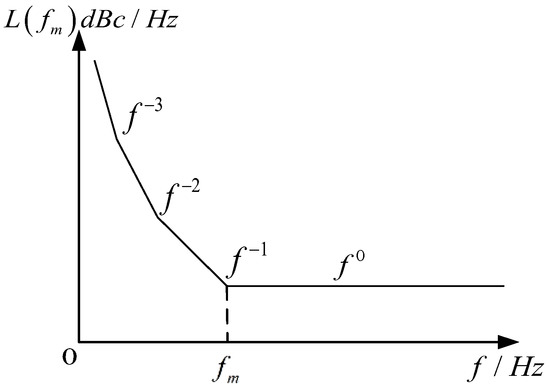
Figure 1. Oscillator characteristic diagram.

Phase noise is parasitic on the signal. It can be described as the ratio of the power of an oscillator signal within the 1 Hz bandwidth at an offset frequency $f_m$ to the power of the carrier signal and denoted $L\left(f_m\right)$.

A radar signal is a complex signal; however, the properties of its real and imaginary parts are the same. For the convenience of analysis, only the real part of the signal is taken for analysis. The mathematical expression of the real part of the LFM signal is as follows:

$$s(t)=A\sin (2\pi f_{0}t+\pi \alpha t^2+{\phi }_0), 0<t<\tau$$

(4)

$\beta$ is the coefficient of phase modulation, and $f_m$ is the coefficient of frequency modulation. If the initial phase of the signal is 0, the LFM signal with phase noise is expressed as follows:

$$s(t)=A\sin [2\pi f_{0}t+\pi \alpha t^2+\beta \sin (2\pi f_{m}t)],0<t<\tau$$

(5)

The following formula can be obtained by the sum formula and Bessel expansion:

$$\begin{array}{c}S\left(t\right)=A\sin \left(2\pi f_{c}t+\alpha \pi t^2\right)+{\displaystyle \sum _{n=1}^{\infty }\frac{\beta }{2}}A\sin \left[2\pi t\left(f_c+\frac{\alpha t}{2}+f_m\right)\right]\\ -{\displaystyle \sum _{n=1}^{\infty }\frac{\beta }{2}}A\sin \left[2\pi t\left(f_c+\frac{\alpha t}{2}-f_m\right)\right]\end{array}$$

(6)

In practice, the coefficient of frequency modulation $f_m$ is a set of frequency offsets, while the coefficient of phase modulation $\beta$ is a corresponding set of values.

2.4. Knowledge Graph

Google formally put forward the concept of the knowledge graph (KG) in May 2012 [33]. Its original intention was to optimize the results returned by search engines, transform the search based on search keywords into the search object itself, and enhance users’ search quality and experience. The knowledge graph is mainly divided into general and domain knowledge graphs [34]. For the general knowledge graph, four large-scale knowledge bases, including Freebase, Wikidata, DBpedia and YAGO, are at the core [35,36]. They provide essential data support for intelligent searches and personalized recommendations of common sense. The domain knowledge graphs include the Internet Movie Database (IMDB), MusicBrainz, UMLS and GeneOnto [37,38,39,40]. IMDB is a database about movie actors, movies, TV programs, TV stars and film production [37]. MusicBrainz is a music knowledge base that collects all music metadata [38]. The medical field includes knowledge bases such as UMLS and GeneOnto [39,40]. Then, the domain knowledge graphs in medical care, e-commerce, finance, agriculture and other fields have been effective [19,20,21,22,23]. Pham T proposed a graph-based multi-label disease prediction model, which uses the medical knowledge graph to help identify the connection between different diseases [19]. Experiments showed that their method outperformed the state-of-the-art algorithms. L. Feng proposed a domain knowledge graph in the E-commerce field called AliMe KG [20]. L. Feng applied AliMe KG to several online business scenarios, such as shopping guides, question answering over properties and recommendation reason generation, and gained approving results. Knowledge graph research in various fields has promoted the better development of the field.

The knowledge graph is essentially a relational network and a graph-based data structure. Broadly speaking, a knowledge graph describes various entities or concepts and their real-world relationships. It constitutes a vast semantic network graph comprising nodes and edges. Nodes are composed of entities or concepts, while the edges are composed of attributes of entities or relationships among entities. The key to constructing the radar emitter knowledge graph is to model nodes and edges and quantify the attribute values of the edges. The successful application of the KGs motivates us to develop a new framework to organize the recognition information provided by the model.

3. Methods

The current research on intelligent emitter recognition algorithms pays more attention to improving the algorithm performance and the numerical improvement of the recognition rate. The relationship between the data itself and the information implied by the difference in the recognition rate is barely utilized. In addition, for many given recognition tasks, the recognition rate of the algorithm has certain requirements, but it is not the only criterion. Furthermore, it is also required to quickly select and organize the appropriate data to train the recognizer that meets the task index efficiently and quickly. To address the data management problem, the proposed KG-1D-CNN has the following processes, as shown in Figure 2:

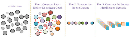
Figure 2. The flow diagram of the proposed KG-1D-CNN. (different colors represent different nodes, datasets and network layers).

• At first, we construct the knowledge graph of the radar emitter. The knowledge graph is used to provide a qualitative and quantitative representation of the relationship between radar data while in the process of radar emitter identification.
• Secondly, a precise dataset of specific tasks is compiled. For the specific recognition tasks, we performed data selection and identification difficulty ranking based on the constructed knowledge graph to construct the precise dataset.
• Thirdly, we constructed a radar emitter identification network based on the knowledge graph. On the basis of the selected training data (precise dataset), the network is adjusted so that it can identify targets from simple to complex based on prior knowledge.

3.1. Construct Radar Emitter Knowledge Graph

Other knowledge graphs aim to describe various entities (nodes) and their relationships (edges) in the real world. However, the radar emitter knowledge graph is actually used to measure the magnitude of difference between different emitter data; that is, to characterize the degree of recognition difficulty among radar emitter individuals. For clarity, some terms need to be explained:

• Node: In graph structures, a node is a vertex in a graph. The knowledge graph expands on the graph’s basis, and a node is a vertex composed of entities and concepts.
• Edge: In a graph, an edge is a line between nodes. In the knowledge graph, edges represent the connections between nodes, comprising relationships and attributes.
• Radar emitter individual: the radar emitter individual is a unique radar with fingerprint characteristics, and all emitters mentioned in this paper refer to the radar emitter.

The reasonable selection and application of radar data depend on the analysis of data relationships. In this paper, the knowledge graph of radar emitters is defined as the recognition relationship between radar data regarding a certain model. The key to constructing the emitter’s knowledge graph is to model the construction of nodes and edges. As shown in Figure 3, the construction of the knowledge graph in this section consists primarily of three steps.

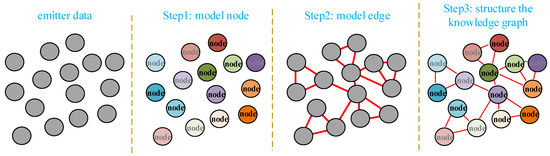
Figure 3. The flow diagram of the construction of the radar emitter knowledge graph. (different colors represent different nodes).

• Step 1: Node Modeling: this section primarily implements the mapping of radar data to the nodes in the knowledge graph.
• Step 2: Edge Modeling: the relationship between radar data is materialized as the edges between nodes, and the proposed measure model is used for qualitative and quantitative measurements.
• Step 3: Radar Emitter Knowledge Graph Construction: by integrating the results of step 1 and step 2, a radar emitter knowledge graph is formed to represent the interaction between radar data during the radar identification process.

3.1.1. Node

Node modeling and edge modeling are the basis for knowledge graph construction. This section uses node modeling to implement the representation of radar emitter data in the knowledge graph. The knowledge graph in this article primarily describes the relationship between radar data. Typically, the dataset originating from the same radar individual can represent the radar individual at the data level. The relationship between the radar individuals and samples fits the connotation of entities and concepts in node definition. Therefore, the radar individual is modeled as a node in the knowledge graph. Specifically, the radar dataset representing the radar individual is used as the filling content of the individual radar node. The specific node construction process is shown in Figure 4.

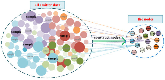
Figure 4. The node construction flow diagram of the radar emitter knowledge graph. (different colors represent different samples and nodes).

The preceding diagram demonstrates that the radar data samples are modeled as distinct nodes in the knowledge graph via node construction. The comprehensive algorithm for node construction is shown in Algorithm 1.

Algorithm 1: The Nodes Construction Algorithm

$\begin{array}{ll}1:& \mathbf{Input}: \mathrm{radar} \mathrm{emitter} \mathrm{datasets}: dataset{s}_1,dataset{s}_2,\cdots ,dataset{s}_k.\\ 2:& \mathbf{Output}:\mathrm{the} \mathrm{node}-\mathrm{set} \mathrm{of} \mathrm{radar} \mathrm{emitter} \mathrm{knowledge} \mathrm{graph}: V\\ 3:& \mathrm{Construct} \mathrm{the} \mathrm{radar} \mathrm{emitter} \mathrm{nodes} \\ 4:& \mathbf{for} i=1 \mathrm{to} k \mathbf{do} // k:\mathrm{the} \mathrm{number} \mathrm{of} \mathrm{radar} \mathrm{emitter}\\ 5:& V_i(n_i\leftarrow rada{r}_i,c_i\leftarrow datase{t}_i) // n_i:\mathrm{the} \mathrm{name} \mathrm{of} V_i, c_i:\mathrm{the} \mathrm{content} \mathrm{of} V_i\\ 6:& \mathbf{end}\mathbf{for}\\ 7:& \mathbf{return}V\end{array}$

3.1.2. Edge

In the section, when using edge models, the relationships between radar data are modeled. Unlike the previous radar emitter identification process that is based on multi-parameter measurements and time-frequency analysis, this paper’s specific radar emitter identification is based on the full-pulse radar data of the intermediate frequency, and it is unnecessary to measure and analyze the attributes of radar data samples. The primary purpose of constructing the radar emitter knowledge graph is to measure the relationship between radar emitter data. Undoubtedly, there is a relationship between radar emitter data. In the recognition network, data interaction influences the training and ultimate recognition results of the recognizer. It is easy to find that some data collaboration can improve recognition performance during actual training, while others can make recognition more difficult. For recognition tasks, different data combinations have different effects on the task results, reflecting the collaborative relationship between data, which provides a feasible idea for measuring the relationship between radar data.

This paper models the relationships between radar data using a description of the relationships between nodes in the signed network [41]. A signed network is a two-dimensional complex network using nodes and edges to express the connection of things. The signed network defines the edges between nodes in two opposite relationships: a positive relationship and a negative relationship. However, the signed network only describes the node relationship qualitatively, and its description accuracy is too low to effectively show the difference in radar data influences on the recognition task. Therefore, based on its concept, the value of the edge is processed continuously. In a given network with N nodes, the definition of edge $e_{ij}$ is as follows:

$$e_{ij}=\left\{\begin{array}{cc}(0,+1)& \mathrm{if} \mathrm{node} v_i \mathrm{to} v_j \mathrm{is} \mathrm{linked} \mathrm{positively}, \hfill \\ (-1, 0)& \mathrm{if} \mathrm{node} v_i \mathrm{to} v_j \mathrm{is} \mathrm{linked} \mathrm{negatively}, \hfill \\ 0& \mathrm{if} \mathrm{node} v_i \mathrm{and} v_j \mathrm{is} \mathrm{linked} \mathrm{weakly}. \hfill \end{array}\right.$$

(7)

where, $e_{ij}$ is the edge of the node $v_i$ pointing to the node $v_j$. It should be noted that $e_{ij}$ is different from $e_{ji}$.

Data drives the application of intelligent networks in radar emitter identification; therefore, whether the data contribute to completing the identification task is a qualitative criterion for its positive and negative relationships. The interaction of data causes the result of emitter recognition, and the emitter recognition rate is its numerical expression. Thus, a comprehensive analysis of the emitter recognition rate can be used to quantify the interaction between data in this recognition task. The specific measurement algorithm is shown in Algorithm 2.

Algorithm 2: The Edges Quantification Algorithm

$\begin{array}{ll}1: & \mathbf{input}: \mathrm{the} \mathrm{radar} \mathrm{emitter} \mathrm{nodes} : V=\{\cdots ,V_i:(n_i\leftarrow rada{r}_i,c_i\leftarrow datase{t}_i),\cdots \}\\ & N: \mathrm{the} \mathrm{nuber} \mathrm{of} \mathrm{radar} \mathrm{emitter} \mathrm{nodes}\\ 2: & \mathbf{output}:\mathrm{the} \mathrm{edge} \mathrm{set} \mathrm{formed} \mathrm{by} \mathrm{the} \mathrm{nodes} \mathrm{in} V: E=\{\cdots ,e_{ij},\cdots \}\\ 3:& \mathrm{Use} \mathrm{the} \mathrm{emitter} \mathrm{identifier} \mathrm{to} \mathrm{obtain} \mathrm{the} \mathrm{recognition} \mathrm{rate} \mathrm{set} \mathrm{of} \{\cdots ,rada{r}_i,\cdots \} \mathrm{in} V \\ & \mathrm{is} \{\cdots ,p_i,\cdots \}. // \mathrm{Prepare} \mathrm{for} \mathrm{the} \mathrm{edge}’\mathrm{s} \mathrm{quantificaion} \\ 4: & \mathbf{for} i=1 \mathrm{to} N \mathbf{do} // \mathrm{Quantify} \mathrm{the} \mathrm{edge} \mathrm{in} \mathrm{the} \mathrm{graph}\\ 5:& \mathbf{for} j=1 \mathrm{to} N \mathbf{do}\\ 6:& e_{ij}=p_j // \mathrm{Use} \mathrm{the} \mathrm{recognition} \mathrm{rate} \mathrm{to} \mathrm{quantify} \mathrm{the} \mathrm{edge}\\ 7:& \mathbf{if} i=j \mathbf{then}\\ 8:& e_{ij}=None // \mathrm{Correct} \mathrm{the} \mathrm{value} \mathrm{of} \mathrm{edges} \mathrm{pointing} \mathrm{to} \mathrm{itself} \\ 9:& \mathbf{end} \mathbf{if}\\ 10:& \mathbf{end} \mathbf{for}\\ 11:& \mathbf{end} \mathbf{for}\\ 12:& \mathbf{return} E\end{array}$

Through the quantification operations of all edges in the graph, the set of all edge values $e=\left\{\cdots ,e_{ij},\cdots \right\}$ is obtained. Since the recognition rate is a value on the continuous interval $(0,1)$, there is $e_{ij}\in (0,1)$. Locating the values 0, −1 and 1, and in particular, 0 in the threshold, is the key objective of edge value characterization in Formula (7). In this paper, the mean, maximum and minimum values of the set are taken to map 0, −1 and 1 in Formula (7), respectively, using the function $f\left(·\right)$ to achieve their mapping. The specific formula is as follows:

$$\begin{array}{l}\min (e),mean(e),\max (e)\stackrel{f(·)}{\to }-1,0,+1\\ f(e)=\left\{\begin{array}{c}\frac{e-\min (e)}{mean(e)-\min (e)}-1,e<mean(e)\\ \frac{e-mean(e)}{\max (e)-mean(e)}, e\ge mean(e)\end{array}\right.\end{array}$$

(8)

3.1.3. Radar Emitter Knowledge Graph

The recognition accuracy of a radar emitter individual is the result of the interaction of all the training data. The certain target individual’s recognition accuracy is the embodiment of the interactions of the other individuals included in the training set, which can be used to describe the other individuals’ influence on the identification of the individual quantitatively. However, in one recognition task, it is difficult to distinguish the influence degree of other individuals on the target individual. Therefore, this paper subdivides the identification tasks in the building process of the radar emitter knowledge graph and measures the different influence values through multiple identification tasks.

In this paper, the measurement of the edge $e_{ij}$ from node $v_i$ pointing to node $v_j$ is taken as an example. Firstly, the recognition task, including the target node $v_j$, the node $v_i$ and other nodes, is selected to train the recognition network, and the recognition rate is obtained. In a recognition task, the recognition rate of $v_j$ is the edge sub-value $e_{ij}^{\prime }$ from node $v_i$ pointing to node $v_j$ under the interference of this third-party node in this recognition task. Notably, (1) the recognition network is used as the measurement component to provide the recognition rate in this process; (2) the node’s number $K$, including the measured nodes $v_i$ and $v_j$, is set to $K\ge 3$ because at least one third-party node participation is required in one recognition task for measuring the edges. Secondly, all task combinations are to be obtained, including the target nodes and third-party nodes, and the recognition rates of the target nodes under these recognition task conditions are to be counted. Then, we obtain all the edge sub-values $e_{ij}^{\prime }$ from node $v_i$ pointing to node $v_j$ when various influences are introduced in the radar emitter knowledge graph. Thirdly, all the sub-values $e_{ij}^{\prime }$ are averaged, and the ultimate value of edge $e_{ij}$ is the average value, which balances the effects of all the other nodes. Finally, all edges in the radar emitter knowledge graph traverse the above operations. By integrating these edges, the radar emitter knowledge graph’s relational adjacency matrix of nodes is obtained. The specific Algorithm 3 is as follows.

Algorithm 3: Knowledge Graph of Radar Emitter Structuring Algorithm

$\begin{array}{ll}1:& \mathbf{input}: \mathrm{the} \mathrm{radar} \mathrm{emitter} \mathrm{nodes}: V=\{\cdots ,V_i:(n_i\leftarrow rada{r}_i,c_i\leftarrow datase{t}_i),\cdots \}(\mathrm{included} N \\ & \mathrm{nodes}), \mathrm{the} \mathrm{node}’\mathrm{s} \mathrm{number} \mathrm{in} \mathrm{once} \mathrm{recognition} \mathrm{task} \mathrm{for} \mathrm{measuring} \mathrm{edges}: K(K\ge 3)\\ 2:& \mathbf{output}:\mathrm{the} \mathrm{adjacent} \mathrm{matrix} \mathrm{of} \mathrm{radar} \mathrm{emitter} \mathrm{knowledge} \mathrm{graph}: G(V,E) \\ 3:& \mathrm{Divide} \mathrm{the} \mathrm{nodes} \mathrm{into} \mathrm{a} \mathrm{group} \mathrm{of} K \mathrm{nodes}, \mathrm{and} \mathrm{get} \mathrm{all} \mathrm{possible} \mathrm{combinations} \mathrm{as} M, \mathrm{where}\\ & M_t=\{\cdots ,v_j,\cdots \}\in M. // \mathrm{Prepare} \mathrm{node} \mathrm{grouping} \mathrm{for} \mathrm{measuring} \mathrm{edges} \\ 4:& \mathbf{for} M_i=\{\cdots ,v_j,\cdots \}\mathbf{in} M \mathbf{do} // \mathrm{Get} \mathrm{the} \mathrm{measured} \mathrm{values} \mathrm{of} \mathrm{the} \mathrm{edges} \mathrm{in} \mathrm{all} \mathrm{groups} \\ 5:& \mathrm{Train} \mathrm{the} \mathrm{emitter} \mathrm{identifier}\mathrm{with} \{\cdots ,dataset{s}_j,\cdots \} \mathrm{in} M_i, \mathrm{and} \mathrm{obtain} \mathrm{the} \mathrm{recognition} \mathrm{rate} \\ & \mathrm{set} \mathrm{of} \{\cdots ,rada{r}_j,\cdots \} \mathrm{is} \{\cdots ,p_j^i,\cdots \}. // \mathrm{Prepare} \mathrm{for} \mathrm{the} \mathrm{edge}’\mathrm{s} \mathrm{quantificaion} \mathrm{in} M_i\end{array}$

$\begin{array}{ll}6:& \mathbf{for} t \mathbf{in}{M}_i\mathrm{do}\\ 7:& \mathbf{for} q \mathbf{in}{M}_i\mathbf{do}\\ 8:& e_{qt}^i=p_t^i // \mathrm{Use} \mathrm{the} \mathrm{recognition} \mathrm{rate} \mathrm{to} \mathrm{quantify} \mathrm{the} \mathrm{edge} \mathrm{in} M_i\\ 7:& \mathbf{if} i=j \mathbf{then}\\ 8:& e_{tt}^i=None // \mathrm{Correct} \mathrm{the} \mathrm{value} \mathrm{of} \mathrm{edges} \mathrm{pointing} \mathrm{to} \mathrm{itself} \\ 9:& \mathbf{end} \mathbf{if}\\ 9:& \mathbf{end} \mathbf{for}\\ 11:& \mathbf{end} \mathbf{for}\\ 12:& \mathbf{end} \mathbf{for}\\ 13:& e=\frac{1}{C_{N-2}^{K-2}}{\displaystyle \sum _{i=1,\cdots ,C_N^K}{e}^i} // \mathrm{Take} \mathrm{the} \mathrm{average} \mathrm{of} \mathrm{all} \mathrm{measured} \mathrm{values} \mathrm{as} \mathrm{the} \mathrm{final} \mathrm{value} \\ 14:& e=f(e) // \mathrm{Use} \mathrm{formula}\left(8\right) \mathrm{to} \mathrm{map} \mathrm{the} \mathrm{value} \mathrm{of} \mathrm{edges} \mathrm{in} \mathrm{the} \mathrm{graph} \mathrm{to} (-1, 1)\\ 15:& G(V,E), V=\{v_1,\cdots ,v_N\}, E=\{e_{12},\cdots ,e_{(N-1)N}\} // \mathrm{Integrate} V \mathrm{and} E \mathrm{to} \mathrm{get} G\\ 16:& \mathbf{return} G\end{array}$

The above process of building the radar emitter knowledge graph based on radar data can be simply represented in Figure 5.

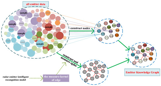
Figure 5. The construction framework diagram of the radar emitter knowledge graph. (different colors represent different samples and nodes).

3.2. Precise Dataset Construction

In the radar information processing system, the specific emitter identification generally trains the recognizer based on the data provided by the front end. The intelligence information on the target of the front-end reconnaissance system is beneficial for radar emitter identification. However, it is usually only sent to the decision-making system to assist in decision-making, while it is not applied to the process of emitter identification. The previous identification process could not extract helpful information and form an effective strategy to improve the identification performance, which resulted in a waste of intelligence information. The actual recognition scene is a complex scene with multiple emitters. Generally, radar emitter recognition usually sends all the training data of the radar emitters without distinction to the intelligent recognition network for recognizer training, which can achieve good results when the data and computing resources are sufficient. However, because the data are not distinguished, the network’s resources are evenly distributed to all types of data. The effective features for identification in the network are screened out little by little through training iteration. Moreover, when many types of data enter the network simultaneously, they often need a deeper network to obtain the required recognition rate. To sum up, the existing problems of the current recognition methods include insufficient use of front-end target information and insufficient consideration of the data differences in recognition network training.

With the above radar emitter knowledge graph, we can obtain the difference values between the data. With the front-end intelligence information and task information, we can obtain the recognition difficulty values between the emitter data. According to the information, the effective part of the knowledge graph is extracted to form a subgraph. Using the subgraph, the data influence relationship between the target node and the task-related nodes can be described.

In the process of learning new knowledge, humans tend to learn key and simple knowledge first, followed by progressively more difficult information until they master the complex new knowledge. In this section, the precise dataset construction method can learn from the human knowledge acquisition process. The specific operation is to arrange all nodes according to the degree of difficulty, distinguishing nodes from target nodes and forming a precise dataset with a difficulty ranking for a specific task. The specific operation process is shown in Figure 6.

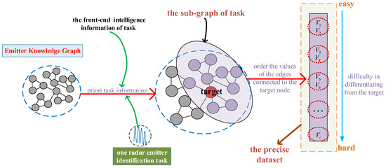
Figure 6. The process diagram of forming the precise dataset.

Compared to the disorderly placement of data and feeding them together into the network, the precise dataset can express the ease of differentiation between different individuals and target individuals, which provides data preparation for further use of the precise dataset for the simple to complex identification of radar emitters.

3.3. The Proposed Specific Emitter Identification Method

3.3.1. Specific Emitter Identification via 1D-CNN

The convolutional neural network has been widely used because of its excellent feature extraction and noise immunity performance [42,43]; therefore, this paper selects CNN as the identification model. Meanwhile, in order to better retain the subtle features of radar individuals and improve the timeliness of the recognition algorithm, this paper selects the radar emitter recognition algorithm based on the IF data. This paper selects 1D-CNN to classify and identify the IF radar data because the radar IF data is a one-dimensional signal.

Our radar emitter identification model is the 1D-CNN, comprising an input layer, convolutional layer, pooling layer, fully connected layer and classifier. Figure 7 shows the structure of the 1D-CNN constructed in this paper. First, the input layer inputs a one-dimensional radar IF data sequence of size 3000 × 1. Then, three blocks of the “convolutional layer + pooling layer” are built. Since the network’s input data is one-dimensional, we use one-dimensional convolutional kernels with the size of 7 × 1. The pooling layer performs the extraction of the main features, and the maximum pooling is chosen here. In addition, the activation functions after the three pooling layers are chosen as the hyperbolic tangent activation function. Finally, a fully connected layer connects the features obtained from the third pooling layer to obtain a vector of size 1 × 96. Dense is used for dimensionality reduction to obtain a vector of size 1 × 10. The vector is sent to the softmax classifier for its final classification.

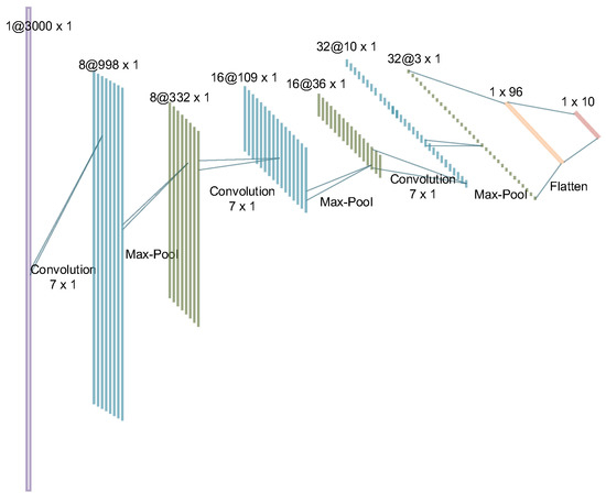
Figure 7. The 1D-CNN structure diagram.

3.3.2. Specific Emitter Identification via Knowledge Graph and 1D-CNN

The previously constructed radar emitter knowledge graph has already laid the foundation for solving the proposed problem, which measures the relationship between the radar data in the knowledge graph and provides a necessary reference basis for selecting and using data in this method. The framework diagram of the proposed method is shown in Figure 8.

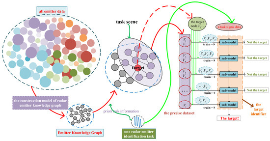
Figure 8. The framework diagram of the proposed method. (different colors represent different radar emitter data).

The method is divided into three main parts: the construction part of the radar emitter knowledge graph, the precise dataset construction part, and the training part of the radar emitter identification network. The first part constructs a radar emitter knowledge graph based on radar data, in the form of which the relationships between radar data are described. The second part is to use the information from the knowledge graph to construct the precise dataset for the specific task. At first, we combine the front-end intelligence information and task information to extract the subgraphs of the radar emitter knowledge graph, which contain the relationships between the target nodes and nodes in the task scene. Then, the nodes are ranked according to the subgraphs to obtain the precise dataset with a recognition difficulty from easy to difficult. The third part is training the recognition network based on the previous research. The network, built on the identification sub-model according to the precise dataset, sifts out the non-target data from easy to difficult. Finally, the data that pass all the sub-models are those predicted to be the target, while vice versa are those predicted to be non-targets. According to the data characteristics and task scene, the final recognition network is built by the sub-models of the same structure. In this paper, the sub-models are chosen as 1D-CNNs because radar emitter identification is performed on the IF data (belonging to one-dimensional data). The specific emitter identification algorithm via KG and 1D-CNN is as follows.

Compared to feeding all the data directly into the network, the proposed method guides the network’s training through a reasonable analysis of the relationships between the radar data. The proposed method uses a precise dataset to hierarchize the recognition difficulty. Recognition sub-models are cascaded to achieve target recognition from easy to difficult, step by step. Each passing sub-model screens out a portion of the non-target data, thus reducing the difficulty of the final task. The task’s difficulty is reduced step by step, and by the last sub-model, the task difficulty has been simplified into layers. The traditional all-in approach needs to continuously fit comprehensive, high-quality features to distinguish all individuals during training. At the same time, in the proposed method, each sub-model tends to learn the significant distinguishing features of the corresponding sub-task. The results of all sub-models are added together to obtain the final recognition results. The task difficulty of the proposed method is the sum of the difficulty of each sub-task. However, the difficulty of the all-into method is geometrically multiplied by the difficulty of all the sub-tasks.

3.4. Computational Complexity Analysis

In this section, the computational complexity of the radar emitter knowledge graph construction algorithm and the KG-1D-CNN algorithm are analyzed. The basic computational composition of both algorithms contains training the 1D-CNN sub-model, and the complexity of the model is mainly described by the model’s parameters and floating-point operations (FLOPs). Since the data size and model structure have been determined, the parameter of a 1D-CNN sub-model is determined to be 5562, and the FLOPs of a 1D-CNN sub-model are also determined to be 3.67 M. Therefore, the complexity of the 1D-CNN sub-model is denoted as $O(B)$, with $B$ being a constant.

The computational complexity of the knowledge graph construction is mainly determined by two parts: the metric part and the edge value computation part. In the first part, the computational complexity is determined by (1) the number of executions of metric operations and (2) the complexity of an operation (that is, the complexity of training a single 1D-CNN sub-model). The knowledge graph contains $N$ nodes, and a single metric requires the $K$ nodes to participate; therefore, the metric experiment is executed by the $T=C_N^K$ times, and its computational complexity is $O(N^K)$; therefore, the computational complexity of the metric part is $O(B\ast N^K)$. The second part is to compute the edge values based on the metric results. For a single edge, the computation is the average of the results of all metric operations associated with it, and its complexity is $O(N-2)$. There are $N^2$ edges to be computed in the knowledge graph; thus, the complexity of the edge value computation is $O\left(N^2\ast \left(N-2\right)\right)\sim O\left(N^3\right)$. In summary, the complexity of the knowledge graph construction is $O\left(N^K\ast B+N^2\ast \left(N-2\right)\right)\sim O\left(N^K\right)$.

The computational complexity of the KG-1D-CNN algorithm is also determined by two main components. The first source of computation is the precise dataset construction part, which ranks the subgraph of the $n$ radar emitters contained in the task environment, and has a computational complexity of $O\left({\left(n-1\right)}^2\right)$. The second part is the model training, which comprises $n-1/k-1$ 1D-CNN sub-models with the same structure as the previous 1D-CNN sub-model; thus, the computational complexity of this part is $O\left(B\ast \left(n-1/k-1\right)\right)$. In conclusion, the computational complexity of the KG-1D-CNN algorithm is $O\left({\left(n-1\right)}^2+B\ast \left(n-1/k-1\right)\right)$. In terms of numbers, a determined CNN model’s computing effort $B$ is significantly more than a given task’s environmental radar number $n$. Therefore, the complexity of the KG-1D-CNN algorithm depends mainly on the second term.

4. Experiments

In this section, we set five test problems to verify the performance of the proposed method from different aspects, using the 1D-CNN algorithm as the baseline algorithm for comparison. In addition, the proposed method is compared with other radar identification methods at different signal-to-noise ratios (SNR) and the number of samples. All experiments are performed on a computer with an Intel 10900K CPU, 64 GB of RAM and an RTX 3070 GPU. The evaluation metrics of the algorithm mainly comprise precision, recall, the F1-score and accuracy, which are defined as follows.

$$\begin{array}{l}precision=\frac{TP}{TP+FP}, recall=\frac{TP}{TP+FN}, accuracy=\frac{TP+TN}{TP+FP+FN+TN}, \\ F1-score=2\times \frac{precision\times recall}{precision+recall}\end{array}$$

(9)

where, $TP$ (True Positive) is the correctly predicted positive; $FP$ (False Negative) is the wrongly predicted positive; $TN$ (True Negative) is the correctly predicted negative; $FN$ (False Positive) is the wrongly predicted negative.

4.1. Experiment Settings

In this part, ten radar individuals are constructed with different types of parameters or individual parameters. The radar-type parameters are mainly carrier frequencies, frequency bandwidths and time widths, while the individual radar parameters are mainly phase noise parameters and envelope parameters. Since we use filters to simulate the envelope shape, the envelope parameters are mainly expressed as filter parameters. The sampling frequency of all signals is 1 GHz. Ten radar emitters contain different values of SNR of 0 dB, 5 dB, 10 dB and 15 dB, respectively. The number of samples per radar emitter individual dataset with each SNR is 200 and 400, separately. The ten emitter-type parameters and individual parameters are shown in Table 1 and Table 2, respectively.

Table 1. Specific type parameters of 10 radar emitters.

	Carrier Frequency	Frequency Bandwidth	Time Width
Emitter 1	10 GHz	30 MHz	3 μs
Emitter 2	10 GHz	30 MHz	3 μs
Emitter 3	10 GHz	30 MHz	3 μs
Emitter 4	8 GHz	20 MHz	3 μs
Emitter 5	8 GHz	20 MHz	3 μs
Emitter 6	8 GHz	20 MHz	3 μs
Emitter 7	12 GHz	40 MHz	3 μs
Emitter 8	12 GHz	40 MHz	3 μs
Emitter 9	12 GHz	40 MHz	3 μs
Emitter 10	11 GHz	50 MHz	3 μs

Table 2. Specific individual parameters of 10 radar emitters.

	Phase Noise Parameters		Filter Parameters
	Frequency Offset	Phase Noise Coefficient	Sampling Frequency	Cutoff Frequency
Emitter 1	$[1, 10, 100, 2000, 10,000]\cdot$1 kHz	$[1, 0.1, 0.01, 0.004, 0.0003]$	20 kHz	200 Hz
Emitter 2	$[1, 10, 100, 1000, 10,000]\cdot$1 kHz	$[0.5, 0.1, 0.03, 0.008, 0.0004]$	30 kHz	150 Hz
Emitter 3	$[1, 10, 100, 1000, 10,000]\cdot$1 kHz	$[0.1, 0.05, 0.01, 0.007, 0.0008]$	30 kHz	200 Hz
Emitter 4	$[1, 10, 100, 2000, 10,000]\cdot$1 kHz	$[1, 0.1, 0.01, 0.004, 0.0003]$	20 kHz	200 Hz
Emitter 5	$[1, 10, 100, 1000, \mathrm{10,000}]\cdot$1 kHz	$[0.5, 0.1, 0.03, 0.008, 0.0004]$	30 kHz	150 Hz
Emitter 6	$[1, 10, 100, 1000, 10,000]\cdot$1 kHz	$[0.1, 0.05, 0.01, 0.007, 0.0008]$	30 kHz	200 Hz
Emitter 7	$[1, 10, 100, 2000, 10,000]\cdot$1 kHz	$[1, 0.1, 0.01, 0.004, 0.0003]$	20 kHz	200 Hz
Emitter 8	$[1, 10, 100, 1000, 10,000]\cdot$1 kHz	$[0.5, 0.1, 0.03, 0.008, 0.0004]$	30 kHz	150 Hz
Emitter 9	$[1, 10, 100, 1000, 10,000]\cdot$1 kHz	$[0.1, 0.05, 0.01, 0.007, 0.0008]$	30 kHz	200 Hz
Emitter 10	$[1, 10, 100, 1000, 20,000]\cdot$1 kHz	$[1, 0.1, 0.03, 0.007, 0.0002]$	20 kHz	100 Hz

The Figure 9 shows the signal waveforms of 10 radar emitter individuals with the SNR of 10 dB.

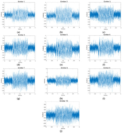
Figure 9. The radar emitter signals of ten radar individuals. (a) Emitter 1; (b) Emitter 2; (c) Emitter 3; (d) Emitter 4; (e) Emitter 5; (f) Emitter 6; (g) Emitter 7; (h) Emitter 8; (i) Emitter 9; (j) Emitter 10.

We designed five recognition problems with the same radar database and SNR of 10 dB. The database contains ten emitters, each with 200 samples. The task’s target individual and interfering individuals in the task environment can be changed to verify the algorithm performance in various task scenes. The five test recognition problems are as follows (Table 3).

Table 3. Details of the five test problems.

Test Problem	Target	Environment	Features
Problem 1	Emitter 7	(Emitter 1, Emitter 4, Emitter 6, Emitter 7, Emitter 8, Emitter9)	Give one target emitter to test the algorithm’s ability in single-target problems.
Problem 2	Emitter 4		Change the target emitter to test the algorithm’s ability in different targets.
Problem 3	Emitter 4, Emitter 7		Give one more target (two targets) to test the algorithm’s ability in multi-target problems.
Problem 4	Emitter 7	(Emitter 1—Emitter 10)	Give more environment emitters (10 emitters total) to test the algorithm’s ability in more complex environments.
Problem 5	Emitter 1—Emitter 10		No prior information to clarify the target to test the algorithm’s ability to identify all the emitters in the complex environment.

In training the network, we used the cross-entropy loss function and Adam optimizer with a learning rate of 0.001 and a batch size of 64. The model with the highest accuracy on the validation set was saved.

4.2. Construction Experiment of Radar Emitter Knowledge Graph

The experimental scenes of five test problems contain the same radar database; therefore, the same radar emitter knowledge graph is constructed. As described in the construction process in Section 3.1, the measure-kernel is constructed using the 1D-CNN network proposed in Section 3.3.1. The number of nodes for each measurement experiment in the edge measure process is chosen as $K=3$. The adjacency matrix of the final radar emitter knowledge graph, obtained from the measurement experiments, is shown in Table 4.

Table 4. The adjacent matrix of radar emitter knowledge graph of the five test problems in Table 3.

	1	2	3	4	5	6	7	8	9	10
1	—	0.40	−0.67	0.90	0.75	0.48	0.71	0.89	0.56	1.00
2	0.53	—	−0.47	0.90	0.77	0.75	0.74	0.77	0.78	1.00
3	−0.34	−0.45	—	0.83	0.53	0.66	0.73	0.83	0.36	1.00
4	0.83	0.73	0.66	—	0.46	−1.00	0.57	0.75	0.59	1.00
5	0.75	0.93	0.62	0.48	—	−0.31	0.61	0.78	0.73	1.00
6	0.83	0.84	0.71	0.04	−0.66	—	0.61	0.84	0.77	1.00
7	0.74	0.63	0.67	0.83	0.85	0.75	—	0.58	−0.75	1.00
8	0.73	0.74	0.56	0.71	0.69	0.90	0.68	—	−0.65	1.00
9	0.86	0.93	0.50	0.83	0.76	0.77	−0.89	−0.10	—	1.00
10	0.83	0.48	0.84	0.79	0.73	0.28	0.85	0.83	0.76	—

The nodes and elements in the adjacency matrix A correspond to the nodes and edges in the knowledge graph $G$, respectively. The correspondence is as follows:

$$a_{ij}=e_{ij} a_{ij}\in A,e_{ij}\in E,v_i,v_j\in V$$

(10)

4.3. Results

The experimental process is divided into the following three main steps.

• First, as in Section 3.2, we extract the task-related subgraph according to the task scene, and the specific formula for extraction is as follows:

  $$\begin{array}{l}{G}_{sub}(V_{sub},E_{sub})\in G(V,E)\\ v_t,v_i\in V_{sub}{v}_t:\mathrm{target} \mathrm{node}, v_i:\mathrm{node} \mathrm{in} \mathrm{the} \mathrm{scene}\\ e_{ti}\in E_{sub}\end{array}$$

  (11)
• Second, the task subgraph is ranked from easy to difficult to construct the corresponding precise dataset for the target.
• Third, the precise dataset is divided into a training set and a test set. In all the subsequent experiments, the number ratio of the training data to test the data is 8:2, and 1/8 of the training data is used as the validation data. As in Algorithm 4, the training set is fed into the network for training to obtain a well-trained recognition model. Finally, the test set is fed into the recognition model to obtain the recognition accuracy.

  Algorithm 4: Specific Emitter Identification via KG and 1D-CNN Algorithm

  $\begin{array}{ll}1:& \mathbf{input}: V: \mathrm{the} \mathrm{dataset} V=v_T+\{v_1,v_2,\cdots ,v_n\} (\mathrm{including} n+1 \mathrm{nodes} \mathrm{and} N \mathrm{data} \mathrm{samples} \mathrm{per} \mathrm{node}\\ & \mathrm{in} \mathrm{the} \mathrm{task} \mathrm{scene}), v_T: \mathrm{the} \mathrm{target} \mathrm{node}, \{v_1,v_2,\cdots ,v_n\}: \mathrm{the} \mathrm{precise} \mathrm{dataset}, \mathrm{the} \mathrm{node}’\mathrm{s} \mathrm{number} \mathrm{in} \mathrm{a}\\ & \mathrm{recognition} \mathrm{identification} \mathrm{sub}-\mathrm{model} \mathrm{training}: k(k\ge 3). \lambda : \mathrm{training} \mathrm{ratio} (\mathrm{the} \mathrm{percentage} \mathrm{of}\\ & \mathrm{training} \mathrm{data} \mathrm{to} \mathrm{total} \mathrm{data}). {\lambda }_1: \mathrm{validation} \mathrm{ratio} (\mathrm{the} \mathrm{percentage} \mathrm{of} \mathrm{validation} \mathrm{data} \mathrm{to} \mathrm{total} \mathrm{data}).\\ 2:& \mathbf{output}: \mathrm{the} \mathrm{trained} \mathrm{identification} \mathrm{network} \\ 3:& \mathrm{Data} \mathrm{partition}:V_t=\{V_{tr},V_{tv},V_{te}\}\\ & \mathrm{training} \mathrm{set}: V_{tr}=V(1:\lambda N)=v_T(1:\lambda N^{(T)})+\{v_1(1:\lambda N^{(1)}),v_2(1:\lambda N^{(2)}),\cdots ,v_n(1:\lambda N^{(n)})\}.\\ & \mathrm{validation} \mathrm{set}: V_{tv}=V(\lambda N+1:(\lambda +{\lambda }_1)N).\\ & \mathrm{test} \mathrm{set}: V_{te}=V((\lambda +{\lambda }_1)N+1:N).\\ 4:& \mathbf{for} i=1 \mathrm{to} ⌈n/k-1⌉\mathbf{do} // \mathrm{Train} \mathrm{all} \mathrm{sub}-\mathrm{models} \mathrm{with} \mathrm{the} \mathrm{precise} \mathrm{dataset}\\ 5:& \mathrm{Take} \mathrm{the} \mathrm{most} \mathrm{distinguishable} k-1 \mathrm{nodes} \mathrm{in} \mathrm{the} \mathrm{precise} \mathrm{dataset}, \mathrm{and} \mathrm{combine} \mathrm{them} \\ & \mathrm{with} \mathrm{the} \mathrm{target} \mathrm{node} \mathrm{to} \mathrm{form} \mathrm{the} \mathrm{sub}-\mathrm{model} \mathrm{dataset}: sub\_V_t^i\\ & // \mathrm{Prepare} \mathrm{datasets} \mathrm{for} \mathrm{the} sub-model\left(i\right) \mathrm{training} \\ 6:& \mathrm{Feed} \mathrm{the} \mathrm{sub}-\mathrm{model} \mathrm{with} sub\_V_t^i // \mathrm{Train} \mathrm{the} sub-model(i) \mathrm{with} sub\_V_t^i\\ 7:& \mathbf{do}: \\ 8:& outpu{t}_i=sub-model.model(sub\_V_{tr}^i)\\ & loss=categorical\_crossentropy(outpu{t}_i,L_{tr}^i) // L_{tr}^i \mathrm{is} \mathrm{the} \mathrm{label} \mathrm{of} \mathrm{data}\\ & loss.backward()\\ 9:& \mathbf{While} epoch<g\\ 10:& \mathrm{Validate} \mathrm{the} \mathrm{trained} \mathrm{sub}-\mathrm{models} \mathrm{with} sub\_V_{tv}^i \mathrm{and} \mathrm{obtain} \mathrm{a} \mathrm{well} \mathrm{trained} sub-model(i).\\ 11:& \mathrm{Remove} \mathrm{the} k-1 \mathrm{nodes} \mathrm{that} \mathrm{have} \mathrm{been} \mathrm{trained}. // \mathrm{Update} \mathrm{the} \mathrm{precise} \mathrm{dataset} \\ 12:& \mathbf{end} \mathbf{for}\\ 13:& \mathrm{Connect} \mathrm{all} \mathrm{the} \mathrm{trained} \mathrm{sub}-\mathrm{model} \mathrm{to} \mathrm{obtain} \mathrm{the} \mathrm{well} \mathrm{trained} \mathrm{network}\hat{1} :\\ & \mathrm{The} \mathrm{target} \mathrm{output} \mathrm{channel} \mathrm{of} \mathrm{the} \mathrm{front} \mathrm{sub}-\mathrm{model} \mathrm{is} \mathrm{connected} \mathrm{with} \mathrm{the} \mathrm{input} \mathrm{channel} \mathrm{of}\\ & \mathrm{the} \mathrm{back} \mathrm{sub}-\mathrm{model}. // \mathrm{Connect} \mathrm{all} \mathrm{the} \mathrm{trained} \mathrm{sub}-\mathrm{model}’\mathrm{s} \mathrm{input} \mathrm{and} \mathrm{output}\\ 14:& \mathrm{Test} \mathrm{the} \mathrm{network} \mathrm{with} \mathrm{the} \mathrm{test} \mathrm{set} V_{te}.\\ 15:& \mathbf{return} \mathrm{network}\hat{1}\end{array}$

4.3.1. Experiments on Five Test Problems

We performed experiments based on the five test problems in Table 3 to verify the performance of the proposed algorithm in different situations, and we used 1D-CNN without KG (as in Figure 7) as the baseline method for the comparison.

The experiments were first conducted under Problem 1 to verify the recognition performance of our method for a single task target.

The interfering emitter individuals under Problem 1 are Emitter 1, Emitter 4, Emitter 6, Emitter 8 and Emitter 9, so the subgraph of Problem 1 is extracted from Table 4. The values of the subgraph are sorted from easy to difficult. The result is shown in Table 5.

Table 5. The subgraph of Problem 1 and the sorting result of the subgraph.

The subgraph	1	4	6	7	8	9
	0.71	0.57	0.61	—	0.68	−0.89
The sorting result	1	8	6	4	9	7
	0.71	0.68	0.61	0.57	−0.89	—

Based on the ranking result of Table 5, the training set was extracted, and the recognition model was trained and tested. The experiments were repeated ten times to exclude the chance factors. The final recognition results are listed in the following table.

From Table 6, it can be seen that the proposed method can achieve good recognition accuracy with an SNR of 10 dB in a single-target recognition task. The process of extracting subgraphs and constructing the precise dataset of a task is simple, yet tedious. A similar description is already provided in the previous experiments; thus, this part will not repeat in the later experiments. Repeated experiments of the proposed and baseline methods were performed under five test problems (10 times per method per test problem). The results are mainly presented in terms of recognition accuracy and time usage, as shown in Figure 10.

Table 6. Accuracy and time usage of the proposed method in Problem 1.

Experiment	Precision		Recall		F1-Score		Accuracy	Time (s)
	Non-Target	Target	Non-Target	Target	Non-Target	Target
Experiment 1	99.50	90.24	98.06	97.67	98.75	93.67	97.92	13.04
Experiment 2	98.98	83.72	96.53	94.74	97.74	88.89	96.25	12.15
Experiment 3	100.00	90.48	98.02	100.00	99.00	95.00	98.33	13.29
Experiment 4	98.98	83.72	96.53	94.74	97.74	88.89	96.25	12.60
Experiment 5	99.51	86.49	97.58	96.97	98.54	91.43	97.50	11.86
Experiment 6	100.00	82.22	96.06	100.00	97.99	90.24	96.67	12.12
Experiment 7	100.00	86.11	97.61	100.00	98.79	92.54	97.92	12.44
Experiment 8	99.49	84.44	96.52	97.44	97.98	90.48	96.67	12.61
Experiment 9	100.00	81.82	96.08	100.00	98.00	90.00	96.67	12.24
Experiment 10	100.00	85.71	97.62	100.00	98.80	92.31	97.92	11.72
Average	99.65	85.50	97.06	98.16	98.33	91.35	97.21	12.41

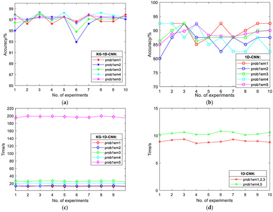
Figure 10. Accuracy and time usage of our method and 1D-CNN in test problems 1–5. (a) Accuracy of our method; (b) accuracy of 1D-CNN method; (c) time usage of our method; (d) time usage of 1D-CNN method.

The results of the repeated experiments were integrated to obtain the results in Table 7. Comparing the results of Problem 1 and Problem 2, it can be seen that our method achieves good recognition results for different targets. For the same target emitter 7, the recognition results are slightly different between Problem 1 and Problem 4; however, their accuracies both reach more than 97%. For the algorithm time usage, the recognition environment of Problem 4 is more complex than Problem 1; thus, the running time spent under Problem 4 is slightly larger than Problem 1. Problem 3 and Problem 5 are designed to verify the performance of the proposed method under the task with multiple recognition targets. The target recognition problem under multiple targets is solved by decomposing it into multiple single-target recognition problems. The results show that the proposed method is also effective for the multiple-target recognition problem. However, the usage time increases as the number of targets increases, which is because the proposed method is more applicable to situations with task-prior information to determine or reduce the range of targets. In addition, the accuracy of the proposed method is higher than that of the baseline method in all five test problems. This indicates that the proposed method of constructing precise datasets based on the radar emitter knowledge graph does help to improve the recognition rate.

Table 7. Accuracy and time usage of the proposed method and baseline method in five test problems (mean of 10 repeated experiments).

Test Problems	1D-CNN		KG-1D-CNN
	Accuracy	Time (s)	Accuracy	Time (s)
Problem 1	90.50	8.98	97.21	12.41
Problem 2	86.50	8.98	96.58	13.52
Problem 3	88.50	8.98	96.90	25.92
Problem 4	87.25	10.41	97.58	19.87
Problem 5	88.80	10.41	97.28	197.23

Since test problem 5 is more complex than the other problems, its results are displayed and analyzed separately next. In test problem 5, the target radar emitters are the same as the environment emitters, simulating the task without a priori information. This is the least suitable case for the proposed method because it is more suitable for tasks with a priori information. The specific experimental results for test problem 5 are as follows:

According to Table 8, the recognition results of ten emitter individuals in Problem 5 differ, with the worst result reaching 95.7%. This difference in recognition merely verifies what is stated previously: there is a difference in the difficulty of recognition between individuals. From Table 1 and Table 2, there is a significant difference between Emitter 10 and the other nine, both in the type parameters and individual parameters; thus, it is the easiest to identify and achieve the highest recognition rate. In this experiment, the overall recognition rate is 97.28% for all the target emitters. We took the sum of each emitter’s time usage as the task time usage, which is 197.23 s.

Table 8. Accuracy and time usage of the proposed method in Problem 5.

Target Emitter	Precision		Recall		F1-Score		Accuracy	Time (s)
	Non-Target	Target	Non-Target	Target	Non-Target	Target
Emitter 1	99.83%	84.88%	97.92%	98.50%	98.86%	90.85%	97.98%	19.91
Emitter 2	99.75%	78.35%	97.02%	97.75%	98.34%	86.92%	97.05%	19.83
Emitter3	98.70%	77.93%	97.21%	88.50%	97.90%	82.69%	96.25%	19.66
Emitter4	99.58%	86.67%	98.33%	96.25%	98.95%	91.17%	98.13%	19.58
Emitter5	99.72%	82.89%	97.70%	97.50%	98.69%	89.47%	97.68%	19.70
Emitter6	98.74%	75.63%	96.47%	88.75%	97.57%	81.05%	95.7%	19.71
Emitter7	98.89%	86.47%	98.42%	90.00%	98.65%	88.08%	97.58%	19.87
Emitter8	99.49%	74.99%	96.39%	95.50%	97.91%	83.89%	96.3%	19.69
Emitter9	98.00%	80.04%	96.90%	82.00%	97.75%	80.90%	96.13%	19.63
Emitter10	100.00%	100.00%	100.00%	100.00%	100.00%	100.00%	100%	19.65
Total	99.27%	82.79%	97.64%	93.48%	98.46%	87.50%	97.28%	197.23

Note: For excluding chance factors of experimental results, each emitter individual identification experiment is performed ten times, and the results in the table are the average of the ten times.

4.3.2. Comparisons with Other Methods

To better demonstrate the effectiveness of our method, this part is compared with some other individual recognition algorithms based on deep learning. The recognition under Problem 5 can be equivalent to the recognition scene of the traditional method, and thus the identification setting of Problem 5 is chosen as the setting of the comparison experiments. The SNR in the scene is changed to observe the change in recognition accuracy with the SNR. The classical RESNET50 is chosen for comparison Algorithm 1. Since this paper recognizes the radar by IF data, which is one-dimensional, the convolution kernel in the network is changed to one dimension, and the network becomes 1D-RESNET50. The algorithms of article [28], article [14] and article [29] are chosen as the comparison Algorithms 2–4. The 1D-CNN mentioned in Section 3.3.1 is chosen for the 5th comparison algorithm. The results of the comparison experiments are as follows:

The recognition accuracy of each method is good when the SNRs are 10 dB and 15 dB. However, with the decrease in SNR, the recognition rates of the five comparison algorithms are significantly reduced. In contrast, the accuracy of the proposed method is slightly reduced with the SNR, and it is still stable above 90%. Although the recognition accuracy of the 1D-CNN algorithm proposed in this paper is slightly lower than that of the comparison algorithms, it takes much less time than all other comparison algorithms. The 1D-CNN makes up for the disadvantage that the proposed algorithm needs more time in the condition to recognize all individuals, so we chose the 1D-CNN as the sub-model of the proposed algorithm. The experiments also show that the proposed method’s recognition accuracy is stable and high under all SNRs but with the most time used to identify all individuals. However, the proposed method is mainly aimed at the situation where prior knowledge can narrow the target. In conjunction with the previous experiments, it is evident that the time usage of the proposed algorithm will be substantially reduced if the target number is decreased.

Table 9 demonstrates that the recognition performance of the comparison algorithms is poor when the SNR is low. Considering that it may be related to the number of samples, we raised the sample number of each individual to 400 under each SNR and conducted the following recognition experiments. The results are as follows:

Table 9. Accuracy and time usage of traditional methods and the proposed method in different SNR conditions.

SNR	1D-RESNET50		CNN-Man [28]		CNN-Xiao [14]		CNN-Kevin [29]		1D-CNN		KG-1D-CNN
	Accuracy	Time (s)	Accuracy	Time (s)	Accuracy	Time (s)	Accuracy	Time (s)	Accuracy	Time (s)	Accuracy	Time (s)
0 dB	50.20%	154.91	56.55%	15.8	52.75%	28.40	53.48%	31.60	51.00%	10.67	91.86%	200.42
5 dB	70.55%	154.17	74.70%	16.02	73.5%	27.91	74.53%	31.62	71.15%	10.24	95.33%	200.65
10 dB	92.70%	154.67	93.35%	16.04	93.80%	28.23	93.58%	31.38	88.80%	10.41	97.28%	197.23
15 dB	97.98%	154.49	99.95%	16.13	98.90%	29.77	99.25%	30.20	97.75%	10.13	99.35%	205.44

Note 1: All recognition accuracies above are the average results of 10 experiments. Note 2: The knowledge graphs in KG-1D-CNN have been reconstructed because the datasets are different for different SNRs, and the construction process will not be described repeatedly.

Table 10 shows the amount of data that increases; the recognition accuracy of each algorithm increases, and so does the recognition time. The overall recognition of each algorithm with a sample number of 400 is consistent with the sample number of 200. The proposed method can stabilize the recognition accuracy at a high level.

Table 10. Accuracy and time usage of traditional methods and the proposed method using 400 samples per emitter.

SNR	1D-RESNET50		CNN-Man [28]		CNN-Xiao		CNN-Kevin		1D-CNN		KG-1D-CNN
	Accuracy	Time (s)	Accuracy	Time (s)	Accuracy	Time (s)	Accuracy	Time (s)	Accuracy	Time (s)	Accuracy	Time (s)
0 dB	58.33%	294.90	64.13%	26.14	59.00%	49.47	59.28%	56.51	56.73%	16.61	93.30%	310.59
5 dB	79.00%	295.89	81.75%	26.40	79.43%	49.44	80.84%	57.00	73.55%	16.06	95.47%	320.85
10 dB	95.25%	295.96	98.55%	26.34	96.28%	49.84	96.40%	56.22	93.48%	16.27	98.62%	314.98
15 dB	99.25%	296.16	100.00%	26.09	99.94%	51.49	99.37%	57.18	99.33%	16.76	99.70%	310.52

Note 1: All recognition accuracies above are the average results of 10 experiments. Note 2: The knowledge graphs in KG-1D-CNN have been reconstructed because of the change in the sample number of the dataset, and the construction process will not be shown here.

Comparing all the experimental results, we can see that the recognition performances of other traditional recognition algorithms decrease significantly with a smaller sample number and low SNR. At the same time, our method can maintain a high recognition accuracy. Our proposed method measures the influence relationship between the radar data in the recognition task via a knowledge graph, extracts the corresponding subgraph of the specific task and analyzes the influence relationship to guide the network from easy to difficult to identify different emitter individuals. The experiments demonstrate that this recognition approach has good recognition performance in various test scenes.

5. Conclusions

In this paper, we propose a radar emitter identification method based on the radar relationship knowledge graph, which has (1) measured the relationship between radar data, (2) improved the identification accuracy by training the network based on the knowledge graph, and (3) ensured the identification accuracy with fewer data samples and a lower SNR. In this paper, a knowledge graph is used to represent the relationship between radar emitters, where 1D-CNN is used as the metric kernel of the relationship between the nodes in the knowledge graph. The knowledge graph is used to rank the recognition difficulty levels on the task dataset, and the ranked data are fed from easy to difficult to train the sub-models, which are used to build the recognition network to realize the recognition task. The experimental results show that this method could improve the recognition rate. Compared with other recognition methods, it also had better robustness to noise and had more stable recognition results with fewer data.

However, there are some limits to our method. First, the construction of the radar relationship knowledge graph is time-consuming. Secondly, this paper mainly verifies the methodology’s feasibility; thus, the number of radar emitters is not large. Thirdly, the proposed method’s time usage without a priori information is not less than the comparison algorithms. For the first limit, the “offline + online” model is currently used to solve it, in which the knowledge graph’s generation is carried out offline in the early stage. For the second problem, we will expand the radar emitter’s number and explore the characteristics of a larger radar relationship knowledge graph in the future. For the third problem, in future work, we will continue to explore a combined method of knowledge graphs and radar emitter identification that relies little on a priori information.

References

- Zohuri, B. Electronic countermeasure and electronic counter-countermeasure. In Radar Energy Warfare and the Challenges of Stealth Technology; Springer: Berlin/Heidelberg, Germany, 2020; pp. 111–145. [Google Scholar]
- Cao, R.; Cao, J.; Mei, J.-p.; Yin, C.; Huang, X. Radar emitter identification with bispectrum and hierarchical extreme learning machine. Multimed. Tools Appl. 2019, 78, 28953–28970. [Google Scholar] [CrossRef]
- Ting, C.; Wei, G.; Bing, S. A new radar emitter recognition method based on pulse sample figure. In Proceedings of the 2011 Eighth International Conference on Fuzzy Systems and Knowledge Discovery (FSKD), Shanghai, China, 26–28 July 2011; pp. 1902–1905. [Google Scholar]
- Jin, Q.; Wang, H.; Yang, K. Radar emitter identification based on EPSD-DFN. In Proceedings of the 2018 IEEE 3rd Advanced Information Technology, Electronic and Automation Control Conference (IAEAC), Chongqing, China, 12–14 October 2018; pp. 360–363. [Google Scholar]
- Matuszewski, J.; Sikorska-Łukasiewicz, K. Neural network application for emitter identification. In Proceedings of the 2017 18th International Radar Symposium (IRS), Prague, Czech Republic, 28–30 June 2017; pp. 1–8. [Google Scholar]
- Dash, D.; Valarmathi, J. Radar Emitter Identification in Multistatic Radar System: A Review. In Proceedings of the International Conference on Automation, Signal Processing, Instrumentation and Control, Singapore, 27–28 February 2021; pp. 2655–2664. [Google Scholar]
- Kong, M.; Zhang, J.; Liu, W.; Zhang, G. Radar emitter identification based on deep convolutional neural network. In Proceedings of the 2018 International Conference on Control, Automation and Information Sciences (ICCAIS), Hangzhou, China, 24–27 October 2018; pp. 309–314. [Google Scholar]
- Wang, J.; Wang, X.; Tian, Y.; Chen, Z.; Chen, Y. A Radar Emitter Recognition Mechanism Based on IFS-Tri-Training Classification Processing. Electronics 2022, 11, 1078. [Google Scholar] [CrossRef]
- Shi, Y.; Zhang, W.; Zhu, M.; Wang, L.; Xu, S. Specific Radar Emitter Identification: A Comprehensive Review. J. Electron. Inf. Technol. 2022, 44, 1–14. [Google Scholar]
- Zhu, M.; Feng, Z.; Zhou, X. A Novel Data-Driven Specific Emitter Identification Feature Based on Machine Cognition. Electronics 2020, 9, 1308. [Google Scholar] [CrossRef]
- Yu, H.-h.; Yan, X.-p.; Liu, S.-k.; Li, P.; Hao, X.-h. Radar emitter multi-label recognition based on residual network. Def. Technol. 2021, 18, 410–417. [Google Scholar]
- Yao, Y.; Yu, L.; Chen, Y. Specific emitter identification based on square integral bispectrum features. In Proceedings of the 2020 IEEE 20th International Conference on Communication Technology (ICCT), Nanning, China, 28–31 October 2020; pp. 1311–1314. [Google Scholar]
- Pan, Y.; Yang, S.; Peng, H.; Li, T.; Wang, W. Specific emitter identification based on deep residual networks. IEEE Access 2019, 7, 54425–54434. [Google Scholar] [CrossRef]
- Xiao, Y.; Wei, X. Specific emitter identification of radar based on one dimensional convolution neural network. J. Phys. Conf. Ser. 2020, 1550, 032114. [Google Scholar] [CrossRef]
- Hinton, G.E.; Osindero, S.; Teh, Y.-W. A fast learning algorithm for deep belief nets. Neural Comput. 2006, 18, 1527–1554. [Google Scholar] [CrossRef]
- Bengio, Y.; Lamblin, P.; Popovici, D.; Larochelle, H. Greedy layer-wise training of deep networks. In Proceedings of the Twentieth Annual Conference on Neural Information Processing Systems, Vancouver, BC, Canada, 4–7 December 2006; Volume 19. [Google Scholar]
- Ranzato, M.A.; Poultney, C.; Chopra, S.; Cun, Y. Efficient learning of sparse representations with an energy-based model. In Advances in Neural Information Processing Systems; MIT Press: Cambridge, MA, USA, 2006; Volume 19. [Google Scholar]
- Singhal, Amit.: Introducing the Knowledge Graph: Things, Not Strings. Google Blog 16, May, 2012. Available online: https://blog.google/products/search/introducing-knowledge-graph-things-not (accessed on 31 May 2023).
- Pham, T.; Tao, X.; Zhang, J.; Yong, J.; Li, Y.; Xie, H. Graph-based multi-label disease prediction model learning from medical data and domain knowledge. Knowl. Based Syst. 2022, 235, 107662. [Google Scholar] [CrossRef]
- Li, F.-L.; Chen, H.; Xu, G.; Qiu, T.; Ji, F.; Zhang, J.; Chen, H. AliMeKG: Domain knowledge graph construction and application in e-commerce. In Proceedings of the 29th ACM International Conference on Information & Knowledge Management, Virtual, 19–23 October 2020; pp. 2581–2588. [Google Scholar]
- Cheng, D.; Yang, F.; Wang, X.; Zhang, Y.; Zhang, L. Knowledge graph-based event embedding framework for financial quantitative investments. In Proceedings of the 43rd International ACM SIGIR Conference on Research and Development in Information Retrieval, Virtual, 25–30 July 2020; pp. 2221–2230. [Google Scholar]
- Chen, Y.; Kuang, J.; Cheng, D.; Zheng, J.; Gao, M.; Zhou, A. AgriKG: An agricultural knowledge graph and its applications. In Proceedings of the International Conference on Database Systems for Advanced Applications, Chiang Mai, Thailand, 22–25 April 2019; pp. 533–537. [Google Scholar]
- Haussmann, S.; Seneviratne, O.; Chen, Y.; Ne’eman, Y.; Codella, J.; Chen, C.-H.; McGuinness, D.L.; Zaki, M.J. FoodKG: A semantics-driven knowledge graph for food recommendation. In Proceedings of the International Semantic Web Conference, Auckland, New Zealand, 26–30 October 2019; pp. 146–162. [Google Scholar]
- Li, L.; Ji, H.-B.; Jiang, L. Quadratic time–frequency analysis and sequential recognition for specific emitter identification. IET Signal Process. 2011, 5, 568–574. [Google Scholar] [CrossRef]
- Yang, L.; Zhang, S.; Xiao, B. Radar emitter signal recognition based on time-frequency analysis. In Proceedings of the IET International Radar Conference 2013, Xi’an, China, 14–16 April 2013; pp. 1–4. [Google Scholar]
- Xiao, Z.; Yan, Z. Radar Emitter Identification Based on Novel Time-Frequency Spectrum and Convolutional Neural Network. IEEE Commun. Lett. 2021, 25, 2634–2638. [Google Scholar] [CrossRef]
- Baldini, G.; Gentile, C. Transient-based internet of things emitter identification using convolutional neural networks and optimized general linear chirplet transform. IEEE Commun. Lett. 2020, 24, 1482–1486. [Google Scholar] [CrossRef]
- Man, P.; Ding, C.; Ren, W.; Xu, G. A Specific Emitter Identification Algorithm under Zero Sample Condition Based on Metric Learning. Remote Sens. 2021, 13, 4919. [Google Scholar] [CrossRef]
- Merchant, K.; Revay, S.; Stantchev, G.; Nousain, B. Deep Learning for RF Device Fingerprinting in Cognitive Communication Networks. IEEE J. Sel. Top. Signal Process. 2018, 12, 160–167. [Google Scholar] [CrossRef]
- Jiang, H.; Guan, W.; Ai, L. Specific radar emitter identification based on a digital channelized receiver. In Proceedings of the 2012 5th International Congress on Image and Signal Processing, Agadir, Morocco, 28–30 June 2012; pp. 1855–1860. [Google Scholar]
- Cheng, F.; Ying, N. Visualization and Re-extraction Technology of 2D Radar Envelope Data. Comput. Mod. 2018, 1, 69–73. [Google Scholar] [CrossRef]
- Herzel, F.; Ergintav, A.; Sun, Y. Phase noise modeling for integrated PLLs in FMCW radar. IEEE Trans. Circuits Syst. II Express Briefs 2013, 60, 137–141. [Google Scholar] [CrossRef]
- Eder, J.S. Knowledge Graph Based Search System. US20120158633A1, 24 February 2012. [Google Scholar]
- Chen, Z.; Wang, Y.; Zhao, B.; Cheng, J.; Zhao, X.; Duan, Z. Knowledge graph completion: A review. IEEE Access 2020, 8, 192435–192456. [Google Scholar] [CrossRef]
- Chen, X.; Jia, S.; Xiang, Y. A review: Knowledge reasoning over knowledge graph. Expert Syst. Appl. 2020, 141, 112948. [Google Scholar] [CrossRef]
- Zheng, D.; Long, Y.; Zhou, Z.; Chen, W.; Li, J.; Tang, Y. Scholar-Course Knowledge Graph Construction Based on Graph Database Storage. In Proceedings of the International Symposium on Emerging Technologies for Education, Zhuhai, China, 11 November 2021; pp. 448–459. [Google Scholar]
- Herr, B.W.; Ke, W.; Hardy, E.; Borner, K. Movies and actors: Mapping the internet movie database. In Proceedings of the 2007 11th International Conference Information Visualization (IV’07), Zurich, Switzerland, 4–6 July 2007; pp. 465–469. [Google Scholar]
- Stutzbach, A.R. MusicBrainz; JSTOR: Ann Arbor, MI, USA, 2011. [Google Scholar]
- Bodenreider, O. The unified medical language system (UMLS): Integrating biomedical terminology. Nucleic Acids Res. 2004, 32, D267–D270. [Google Scholar] [CrossRef]
- Khan, S.; Situ, G.; Decker, K.; Schmidt, C.J. GoFigure: Automated Gene Ontology™ annotation. Bioinformatics 2003, 19, 2484–2485. [Google Scholar] [CrossRef]
- Tang, J.; Chang, Y.; Aggarwal, C.; Liu, H. A survey of signed network mining in social media. ACM Comput. Surv. (CSUR) 2016, 49, 1–37. [Google Scholar] [CrossRef]
- Chen, Y.; Jiang, H.; Li, C.; Jia, X.; Ghamisi, P. Deep feature extraction and classification of hyperspectral images based on convolutional neural networks. IEEE Trans. Geosci. Remote Sens. 2016, 54, 6232–6251. [Google Scholar] [CrossRef]
- Wiatowski, T.; Bölcskei, H. A mathematical theory of deep convolutional neural networks for feature extraction. IEEE Trans. Inf. Theory 2017, 64, 1845–1866. [Google Scholar] [CrossRef]
Disclaimer/Publisher’s Note: The statements, opinions and data contained in all publications are solely those of the individual author(s) and contributor(s) and not of MDPI and/or the editor(s). MDPI and/or the editor(s) disclaim responsibility for any injury to people or property resulting from any ideas, methods, instructions or products referred to in the content. |
© 2023 by the authors. Licensee MDPI, Basel, Switzerland. This article is an open access article distributed under the terms and conditions of the Creative Commons Attribution (CC BY) license (https://creativecommons.org/licenses/by/4.0/).