Article

Prediction Aerospace Software to Detect Solar Activity and the Fast Tracking of Solar Activity Using Remote Sensing Instruments in Orbit

Changchun Institute of Optics, Fine Mechanics and Physics, Chinese Academy of Sciences, Changchun 130033, China
*
Author to whom correspondence should be addressed.
Remote Sens. 2023, 15(13), 3288; https://doi.org/10.3390/rs15133288
Submission received: 25 May 2023 / Revised: 19 June 2023 / Accepted: 23 June 2023 / Published: 27 June 2023

Abstract

:
At present, solar remote sensing instruments face problems regarding the short detection time for solar activity and the need to preheat the electronics before detection. The accurate orbit prediction function ensures that the maximum error of the payload electronics system preheating time is less than 8 s, enabling the electronics to obtain stable and reliable solar remote sensing data, and allowing the prediction function to adapt to the changes in preheating time and the limit position of turntable rotation. To achieve the complete detection of solar activity by a payload in orbit, a turntable with two directions of rotation was accurately controlled to achieve rapid capture and track the Sun’s activity, and the delay time for tracking the Sun successfully was less than 8 s to ensure that the payload made full use of the solar detection time for full detection. The turntable’s tracking error was less than 0.002°, allowing the payload to obtain high-precision solar remote sensing data in orbit. The above methods enable the payload to realize the complete, stable, and high-precision detection of solar activity in orbit for wavelengths ranging approximately from 165 nm to 2400 nm.

1. Introduction

Solar radiation is the fundamental and paramount energy resource for the Earth. It profoundly influences the global environment and climate, exerting a significant impact. Specifically, the impact includes the greenhouse effect, volcanoes, and monsoons [1,2,3,4,5,6,7,8,9,10]. Therefore, investigating the variations in solar radiation holds the key to exploring the potential implications for future climate changes on Earth. Since the 1970s, large-scale development has been carried out on solar remote sensing instruments. The parker solar probe was developed by the National Aeronautics and Space Administration (NASA) and launched in 2018 [11,12,13,14,15,16]; the solar observation instrument (SOLAR) was installed on the International Space Station (ISS) in 2008, and it has three main loads: a solar variation and irradiance monitor (SOVIM) [17,18], a solar spectral irradiance measurement (SOLSPEC) instrument [19,20], and a solar automatic calibration extreme ultraviolet/ultraviolet spectrophotometer (SOL-ACES) [21]; the Solar TErrestrial RElations Observatory (STEREO) was developed by NASA and Johns Hopkins University (JHU) and was launched in 2006. Both the STEREO–A and STEREO–B carried five loads to detect the Sun’s energy. The transition region and coronal explorer (TRACE) was launched by NASA in 1998 and operates in visible (VIS) to far ultraviolet (UV); the Ulysses was developed by NASA and the European Space Agency (ESA) and launched in 1990. The workaround solar probes in scientific research institutions or universities in China was carried out in the early 21st century. Typical satellites include the advanced space-based solar observatory (ASO-S) launched in 2022 [22,23,24,25], which has three main loads: a Ly alpha Solar Telescope (LST), a hard X-ray imager (HXI), and a full-disc vector magnetograph (FMG). The LST was developed by the Changchun Institute of Optics, Fine Mechanics and Physics, Chinese Academy of Sciences (CIOMP). The Chinese Hα Solar Explorer (CHASE) was launched in 2021 [26] and carried the solar space telescope developed by CIOMP. The successful development of these instruments marked China’s official entry into the era of space exploration.
Although human efforts to detect solar radiation cannot stop solar activity, scientists hope to predict solar activity through the detection of different angles and wave bands of the solar spectrum and make positive responses to it. Therefore, the Fengyun-3E satellite carried three solar exploration payloads developed by CIOMP. One of them was a solar irradiance spectrometer operating in the UV to near-infrared (NIR) (165~2400 nm) range, which could track and detect solar activity 14 times a day, accumulating a large amount of scientific data for the study of solar radiation changes.
Since the annual variation in solar spectral irradiance in VIS and NIR bands is only 10−3, the stability of the solar irradiance spectrometer is required to be better than 0.2%/year in orbit [27]. The stability of the spectrometer is determined by electronics, tracking precision, and the optic system. To obtain the required stability and high precision of the detection data from the solar irradiance spectrometer (spectrometer for short) in orbit, the instrument’s electronic hardware needs to be preheated for several minutes before the measurement. The tracking precision is required to be less than 0.1° [28], and the optical components must be stable. The preheating time is determined by the circuit design and was 30 min in this paper. The stability of optical components was beyond the scope of this paper. The preheating time affects the stability of the instrument measurement results. The deviation in preheating time is required to be less than one minute in orbit. The condition of the track and the limited position of the two-dimensional turntable (turntable for short) mean that the solar observation window (SOW) of each track varies continuously with the seasons, and the minimum time is 24 min. It takes approximately 20 min or more to conduct a complete solar spectral detection. Therefore, it is required that the preheating time should be finished and the fast-tracking solar be successfully realized when sunlight enters the SOW. The spectrometer can determine its position in real time instead of minutes later. Therefore, it is difficult to tell when to start preheating. In this paper, a simple and reliable method is proposed for a prediction function to calculate the preheating start time and quickly capture solar activity in orbit. The method can automatically adapt to the difference in preheating time and the rotation range of the turntable in orbit. Due to the complex conditions of the spectrometer, no instruments with similar requirements have been encountered yet, and therefore, there are no similar methods to refer to, although there are papers related to orbit prediction that propose a method to theoretically calculate the solar angle based on broadcast time and the parameters of the orbit [29]. The calculation process is complex, and the prediction error increases with the increase in prediction time. There have not been any scientific applications so far.

2. Materials and Methods

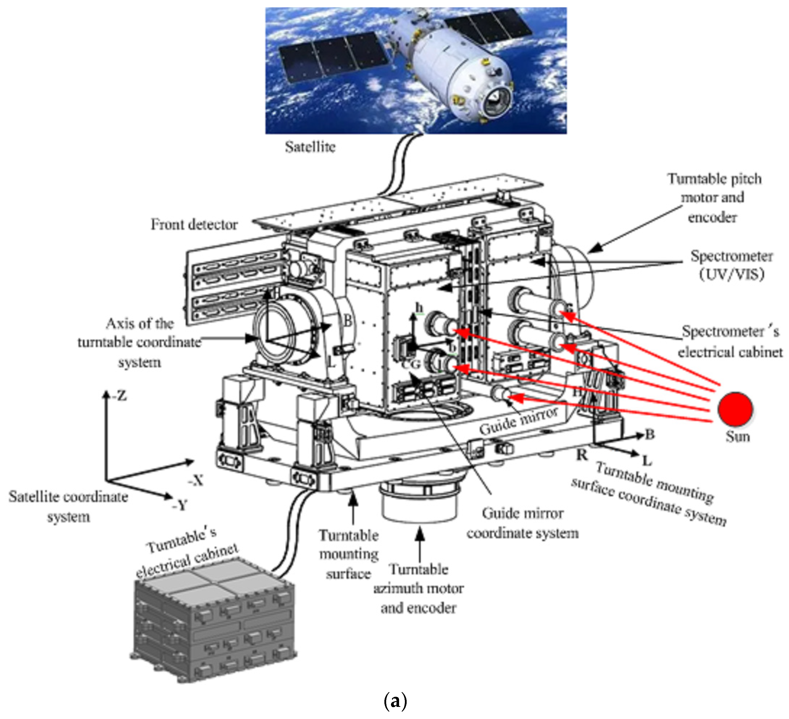
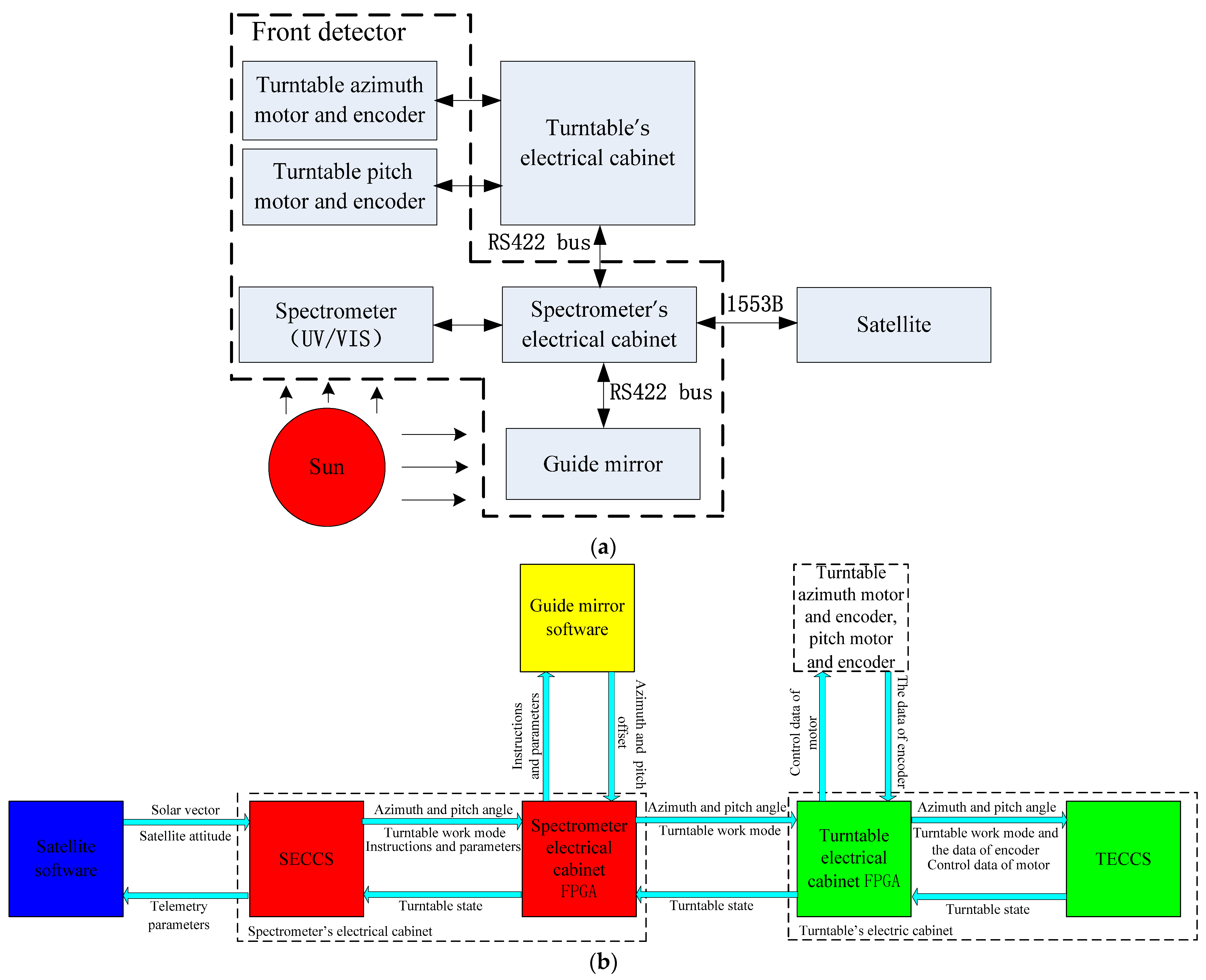
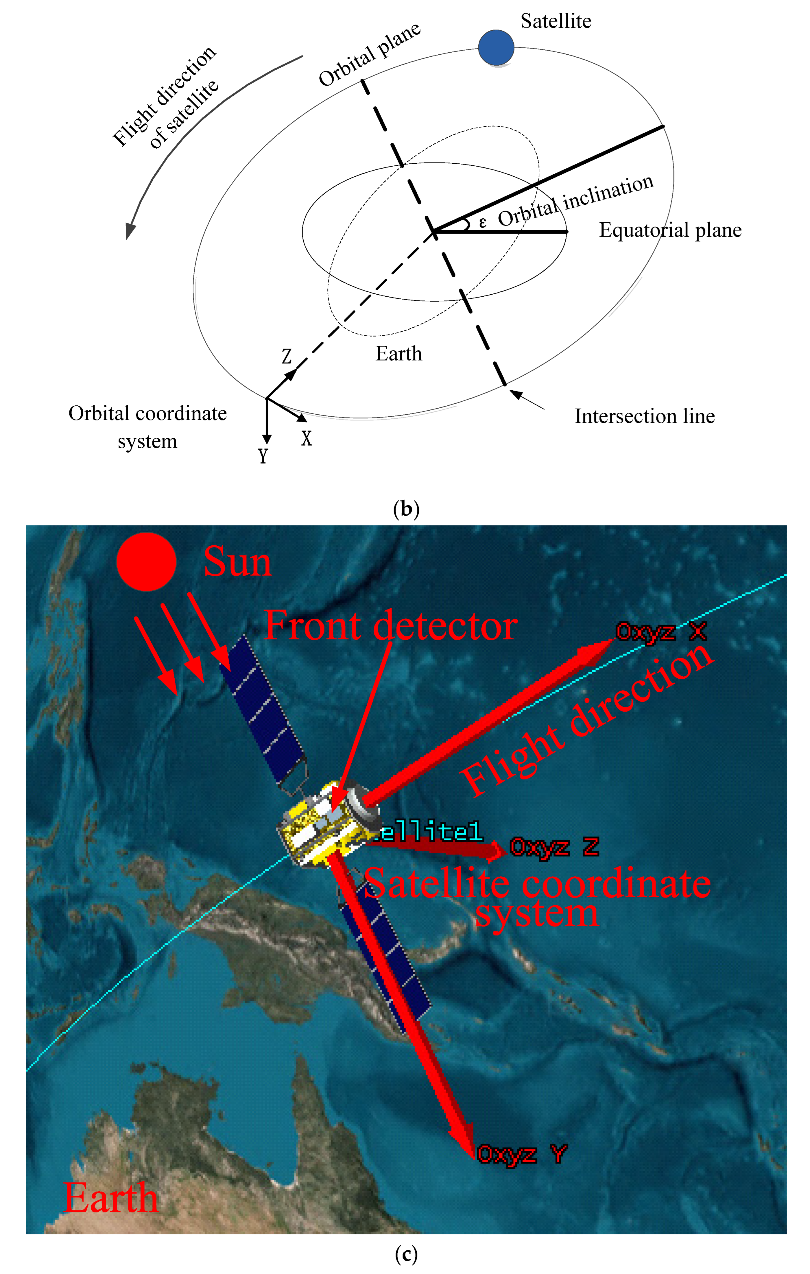
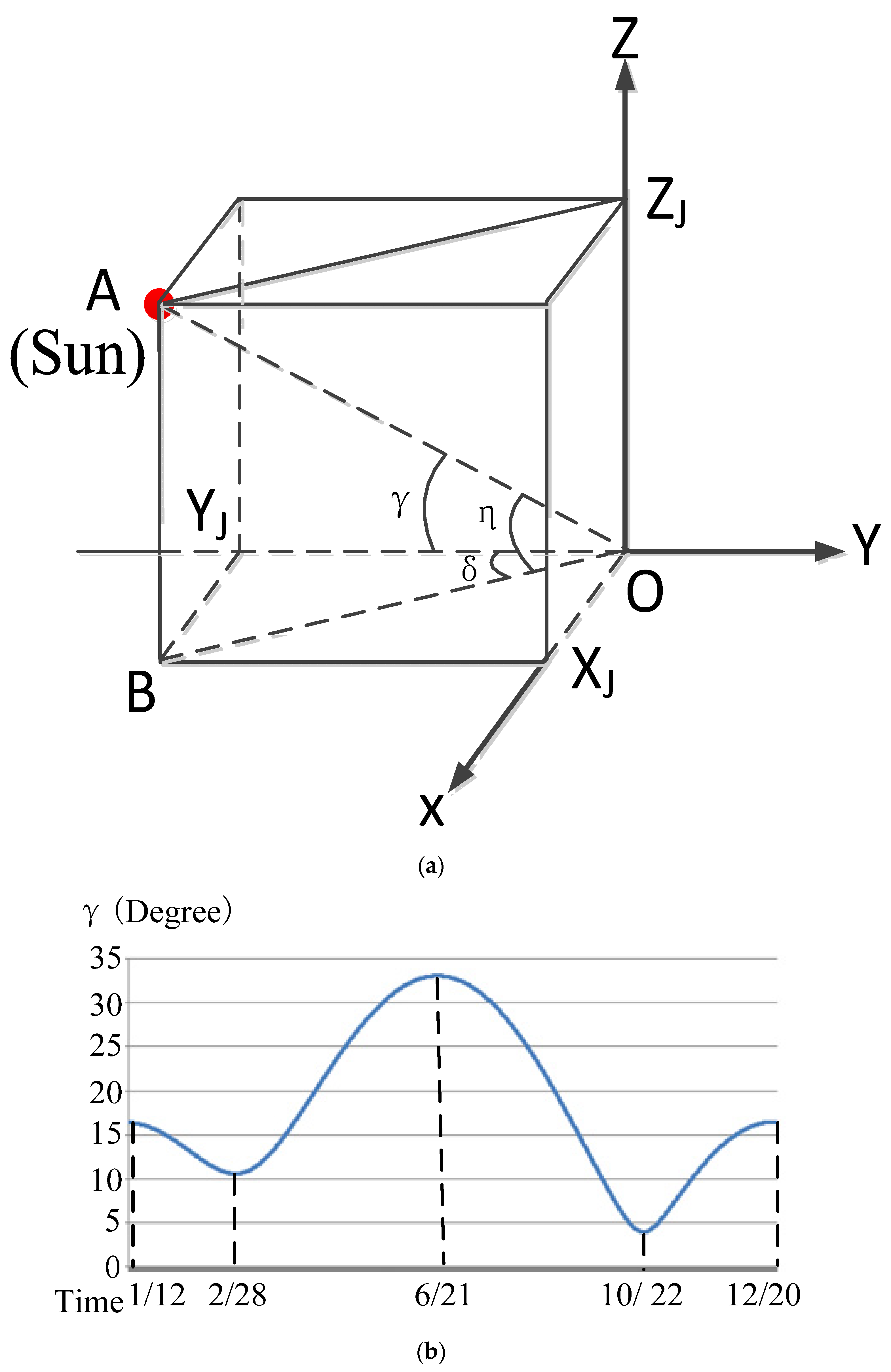
2.1. The Solar Tracking Principle of the Spectrometer

The spectrometer built by CIOMP was loaded on the Fengyun-3E satellite, which started to operate in orbit in 2021. The orbit is characterized by being Sun-synchronous, and the orbital altitude is 850 km. The satellite’s life span is 8 years, and its weight is 6 tons. Because of their long lifetime and heavy weight, the payloads can only adopt the turntable tracking method in orbit [30].
The spectrometer’s composition and the spectrometer and satellite’s coordinate systems are shown in Figure 1a. The spectrometer consists of two parts; one is the turntable’s electrical cabinet (TEC), which controls the rotation of the turntable, and the other is the front detector, which detects the Sun. The abbreviation for the coordinate system is CS. The satellite CS(SCS), turntable mounting surface CS(TMSCS), the axis of the turntable CS(ATCS), and guide mirror CS(GMCS) are theoretically coincident. The orbital CS(OCS) and parameter satellite move around the Earth as shown in Figure 1b. The satellite revolves around the Earth in a Sun-synchronous orbit, as shown. The orbital inclination with respect to the equatorial plane is ε, the value of which is 99°, and this does not affect the prediction function. The orbital cycle is 102 min. The satellite is expected to remain in an orbit with exactly the same orbital parameters throughout its lifetime. For example, the stability of the satellite’s attitude is better than 0.006°. The OCS is as shown too. The position relationship between the Sun, the Earth, and the satellite and the position of the front detector on the satellite is shown in Figure 1c. The satellite moves in the same direction as the +X-axis, the Sun is in the −Y-axis direction and the +Z-axis points towards the Earth. The front detector is on the satellite, on either side of the Earth. The TEC is inside the satellite. The spectrometer’s internal connection and the connection in relation to the satellite are shown in Figure 2a. The front detector contains a spectrometer’s electrical cabinet (SEC), an electronic detection system (containing UV, VIS, and NIR bands), a guide mirror, a motor, and an encoder in azimuth and pitch directions, with all of the above installed on the turntable. The SEC receives data from the satellite and sends angles to the TEC for controlling the turntable.
The satellite and SEC CPU software (SECCS, The version number is 2.05) data flow of the turntable control is illustrated in Figure 2b. The SECCS receives the satellite attitude in a broadcast message and the solar vector in an orbit message sent by satellite through the 1553B (Military Standard 1553 bus, a standard for communications that was developed by the United States Department of Defense) [31,32,33,34]. Using these data and the mechanical installation matrix, the azimuth and pitch angles of the sunlight at the GMCS are calculated by the SECCS immediately. Firstly, this angle is used to realize the timing for the SEC controlling the electronic detection system for powering on and preheating, and secondly, it is used to realize the moment when the SEC controls the turntable through the TEC to bring the sunlight into the guide mirror’s field of view. The TEC obtains the azimuth and pitch angles according to SEC through the RS422 (its full name is Electrical Characteristics of Balanced Voltage Digital Interface Circuits, published by the ANSI Telecommunication Industry Association/Electronic Industries Association (TIA/EIA) in 1994) [35,36,37] communication bus and makes the turntable rotate according to these angles. The corresponding encoder’s location information is utilized for closed-loop.
If the guide mirror’s function is normal and can be utilized, when the sunlight is at the limited position of the turntable (in other words, at the edge of the guide mirror’s field of view, which is circular with a radius of 1°), then the SEC can control the turntable by bringing it into the limit position, putting the sunlight in the guide mirror’s central field of view quickly. Through this, the sunlight can be captured successfully, the SEC will send the guide mirror tracking mode to the TEC, and then it can control the turntable by using the guide mirror’s offset angles to track the sunlight. If all of the offset angles are less than 0.1°, the SEC will control the electronic detection system to detect the Sun and transmit the data to the satellite platform via the 1553B. The guide mirror transmits the azimuth and pitch offsets to SEC via the RS422 bus, and then it transmits them to the TEC.
In cases where the guide mirror’s functionality is abnormal or not utilized, and the sunlight reaches the limited position of the turntable, the SEC can take charge of positioning the turntable at its limited position. The SEC can then transmit the programmed tracking mode to the TEC, which subsequently ensures continuous sunlight tracking by controlling the turntable’s azimuth and pitch angles. If the difference between the calculated angles in both directions and the position information of the same direction encoder is not more than 0.1°, the SEC can control the electronic detection system to detect the Sun and transmit the data to the satellite platform via the 1553B.

2.2. The Method of Orbit Prediction to Detect Solar Radiation

The spectrometer operates on a solar-synchronous orbit with an orbital period of 102 min. The solar cone (γ), azimuth (δ), and pitch (η) angle schematic diagrams are shown in Figure 3a. The solar cone (γ) is formed by lines OA and OYJ; the angle in the azimuth direction is formed by lines OB and OYJ; and the angle in the pitch direction is formed by lines OA and OB. The yearly variation of the solar cone angle with time is shown in Figure 3b. The range of the solar cone angle is approximately 4–34.5°. It reached its maximum value on June 21 and its minimum on October 22. Due to the mechanical structure, the default electronic limits position in the azimuth and the pitch directions of the turntable are −30° to +24° and −34.5° to 2°, respectively. The range can be changed in orbit. The limit position in the azimuth negative direction of the turntable was altered from −30° to −21°, and in the pitch positive direction, it was altered from 2° to 0° by the injection parameters in orbit. According to the limit position in two directions, the maximum SOW is 51 min. To obtain a stable solar spectral curve, the spectrometer electronics system needs to be preheated for 30 min before solar detection, and the preheating time can be changed in orbit. This requires the SECCS to have an orbit prediction function that can adapt to the difference in the preheating time and the limited position of the turntable in orbit. Under the condition that the limit position of the turntable and the electronics’ preheating time can be changed, it is guaranteed that the electronics will complete the preheating when the spectrometer enters the SOW, and this prediction function is not limited by ε (the orbital inclination).
The orbit prediction of the (N + 1)th according to the Nth orbit and the actual preheating time of the (N + 1)th orbit are shown in Figure 4. The spectrometer executes the corresponding mode according to the number of tracks in orbit. Therefore, when the SECCS works in orbit, it needs to define the starting point of the track to achieve mode switching. In theory, the selection of the orbit starting point is arbitrary. According to the characteristics of the satellite’s real-time position data and for the simple and reliable implementation of the SECCS, the orbit starting point is selected above the equator of the orbit-raising section (point D1 in Figure 4), and the orbit count is +1 when the satellite passes this position. Once the starting point of the orbit has been selected, its physical position will remain unchanged, while the position of the SOW in orbit changes with the seasons. Therefore, the relative position relationship between the starting point of the orbit and the SOW also changes with the seasons. To describe this phenomenon using a simple method, it is assumed that the starting point of the orbit is variable, and the AN and CN points are the starting point and the endpoint of the SOW of the Nth orbit, respectively. That is, the solar angle in the ANCN segment of the Nth orbit is within the rotation range of the turntable. For example, the relative position relationship between the starting point of the orbit and the SOW near December 16 is like the relationship between the D2 point and the ANCN segment, and the relative position relationship near October 2 is like the relationship between the D1 point and the ANCN segment. The change in the relative position does not affect the orbital prediction results.
When the SEC is powered on, the SECCS receives the satellite attitude in a broadcast message and the solar vector in an orbit message in a period of 2 s. At the same time, the orbit message count is +1. The orbit message count increases along the satellite’s running direction. When passing the orbital starting point (point D1 in Figure 4), the SECCS resets the orbit message count to 1. Since the tracking period is 102 min, the maximum orbit message count in one track is 3060. The starting point of the SOW of the Nth track (n = 1, 2, …) is marked as the AN point, and the orbit message count at this point is marked as aN. The SECCS marks the starting point of the SOW. The orbit message counts curve of the orbit at the starting point of the SOW at different orbits from one day in October after the satellite launch is shown in Figure 5. The maximum difference between the orbit message counts aN and aN+1 of the two adjacent orbits at the starting point of the SOW is 1; that is, the maximum corresponding time of the ANAN+1 segment (T1) in Figure 4 is 2 s. The solar synchronous orbits are equipped with this feature, and this feature is independent of the rotation range of the turntable azimuth and pitch direction. The SECCS uses this feature to make orbital predictions, and it is not limited by the orbital inclination. The SECCS calculates the solar angle in real time according to the solar vector data. The aN value is updated according to the rotation range of the turntable azimuth and pitch direction, which are −21°~+24° and −34.5°~0°. The rotation range of the turntable azimuth and pitch direction can be changed in orbit. Different rotation ranges correspond to different positions of the starting point (AN point) of the SOW, and the aN value is different accordingly.
The electronic preheating time of the spectrometer is X (30 by default) minutes. The preheating time X is mainly determined according to the design requirements and the life of the electronic hardware. Considering the orbital period (102 min), the detection time (approximately 20 min), and the implementation difficulty of the software (The version number is 2.05), generally, X can be set from 5 to 80 min. If the time between the BN and AN points is X minutes, the BN point is in the reverse direction of satellite movement, and the orbit message update cycle is 2 s, then the orbit message count bN at the BN point should be as follows: when aN > X 60/2 (X default value is 30), bN = aN–X 60/2; when X 60/2 ≥ aN ≥ 1, bN = 3060–X 60/2 + aN. In other words, the time of the BNAN segment (T2) is 30 min.
The orbit prediction method is to select the BN point as the starting position for the electronic powering on and preheating of the (N + 1)th orbit. Similarly, the BN+1 point is selected as the starting position of the electronic powering on and preheating of the (N + 2)th orbit, and so on. The electronics preheating time is BNEN+1, and EN+1 is the position in which the spectrometer tracks the solar activity successfully. A detailed introduction to the EN+1 point is given in Section 4.
The FN+1 point is the position in which the tracking preparation of the turntable electrical cabinet is completed. The tracking preparation time is the BNFN+1 segment, which is approximately 3 s. The AN+1 point is the starting position of the SOW of the (N + 1)th orbit, where the solar radiation is at the limit position of the turntable. The turntable conducts Sun pre-pointing according to the solar angle calculated by the SECCS in the FN+1AN+1 segment. When the Sun is outside the rotation range of the turntable, the turntable rotates to the extreme angle position in one or two directions and waits for the Sun to enter the range of the turntable. At point HN+1, the Sun enters the range of the turntable and is near the central field of view of the guide mirror, and the azimuth and pitch offsets are less than 0.1°. At the EN+1 point, the SECCS controls the turntable to track the Sun successfully with the guide mirror offset. At this time, the spectrometer starts to detect solar activity.
The actual preheating time of the spectrometer is the BNEN+1 segment. The delay time from the Sun entering the SOW (AN+1 point) to the successful tracking of the Sun (EN+1 point) includes the solar capture process of the AN+1HN+1 segment, and the HN+1EN+1 segment makes the guide mirror tracking successful. The maximum corresponding time of the ANAN+1 segment (T1) in Figure 4 is 2 s. The time of the BNAN segment (T2) is 30 min. The main cycle period of the SECCS (T3) is 0.3 s at most, and the orbit message update cycle (T4) is 2 s. The cycle period of the turntable electrical cabinet CPU software (TECCS, The version number is 2.04) (T5) is 1 ms, and the Sun passing angle (V1) is 0.04° every second. The azimuth and pitch axis of the turntable rotates at the same time, and the speed (V2) is 0.25°/s. After eliminating the installation and other deviations between the coordinate systems, the deviation between the calculated angle and the actual angle (α1) is 0.064°. The actual preheating time is as follows:
BNEN+1 = BNAN + AN+1HN+1 + HN+1EN+1 − ANAN+1
including
BNAN = T2 = 30 min
AN+1HN+1 max = 2T3 + T4 + 2T5 + T4V1/V2 = 2.9 s
AN+1HN+1 min = 2T3 + 2T5 + T4V1/V2 = 0.9 s
HN+1EN+1 = ((2T3 + 2T5 + T4V1/V2) V1 + α1)/V2 = 0.4 s
ANAN+1 = T1 = 2 s
It can be seen from Equations (1)–(5) that
BNEN+1 max = BNAN + AN+1HN+1 max + HN+1EN+1 − ANAN+1 = 30 min + 1.3 s
BNEN+1 min = BNAN + AN+1HN+1 min + HN+1EN+1 − ANAN+1 = 30 min − 0.7 s
Therefore, in theory, the maximum error of spectrometer electronics preheating is 1.3 s. The time AN+1EN+1 from the Sun entering the rotation range of the turntable to tracking successfully via the guide mirror is as follows:
AN+1EN+1 = AN+1HN+1 + HN+1EN+1
According to Equations (2)–(4),
AN+1EN+1 max = AN+1HN+1 max + HN+1EN+1 = 3.3 s
AN+1EN+1 min = AN+1HN+1 min + HN+1EN+1 = 1.3 s
Therefore, theoretically, the maximum and minimum delay time from the Sun entering the extreme position of the turntable to tracking successfully via the guide mirror is 3.3 s and 1.3 s, respectively. As the maximum updating period of the telemetry parameters for the ground and in orbit is 8 s, the measured values of the electronics preheating time error and tracking the Sun delay time are less than 8 s. The GN+1 point is the position where the detection of solar radiation is completed. The solar radiation detection time is the EN+1GN+1 section, which is approximately 20 min. The JN+1 point means that the TECCS controls the turntable to convert to the standby state. The corresponding period for the turntable going to 0° in both the azimuth and pitch directions and entering the standby state is the GN+1JN+1 section, which is related to the turntable position at the end of the detection.

2.3. Fast-Tracking Solar Method

The coordinate systems involved in the calculation of the solar azimuth and pitch angle in the GMCS include the OCS, the SCS, the TMSCS, the ATCS, and the GMCS. Ideally, the five CSs are coincident, but there are deviations in satellite attitude control and mechanical installation. Therefore, the sunlight angle at the GMCS is calculated by the solar vector at the OCS, and the process needs four repetitions of CS transformations. The position relationship between the CSs is shown in Figure 1a,b. Due to the long distance from the Sun to the Earth, the translation of all CSs does not affect the calculation of the sunlight angle. The relationship of the five CSs involved in the calculation of the solar angle is illustrated in Figure 6. The sunlight azimuth and pitch angle are calculated using these rotation angles.
Assume that the axes of all CSs are orthogonal. The solar vector at the OCS is [XS YS ZS], and because of the necessary precision for tracking the Sun, the solar vector is normalized to 1, and it is 16 bits, 1 sign bit, and 15 data bits, meeting XS2 + YS2 + ZS2 = 32,7672. The satellite platform sends the attitude parameters of the satellite to the payload every second; that is, the rotation angles between the SCS and the OCS, and the rotation angle around the Z-axis (yaw angle) is β1, the X-axis (rolling angle) is τ1, and the Y-axis (pitch angle) is σ1, as shown in Figure 6. All CS rotations are in the same order. The solar vector transformation to the SCS is [XB YB ZB], and we can then obtain Equation (8) as follows:
X B Y B Z B = cos β 1 cos σ 1 sin β 1 sin τ 1 sin σ 1 sin β 1 cos σ 1 + cos β 1 sin τ 1 sin σ 1 cos τ 1 sin σ 1 sin β 1 cos τ 1 cos β 1 cos τ 1 sin τ 1 cos β 1 sin σ 1 + sin β 1 sin τ 1 cos σ 1 sin β 1 sin σ 1 cos β 1 sin τ 1 cos σ 1 cos τ 1 cos σ 1 X S Y S Z S
Similarly, the solar vector is [XD YD ZD] in TMSCS; it can be calculated using [XB YB ZB] in SCS, and we then obtain Equation (9) as follows:
X D Y D Z D = cos β 2 cos σ 2 sin β 2 sin τ 2 sin σ 2 sin β 2 cos σ 2 + cos β 2 sin τ 2 sin σ 2 cos τ 2 sin σ 2 sin β 2 cos τ 2 cos β 2 cos τ 2 sin τ 2 cos β 2 sin σ 2 + sin β 2 sin τ 2 cos σ 2 sin β 2 sin σ 2 cos β 2 sin τ 2 cos σ 2 cos τ 2 cos σ 2 X B Y B Z B
Similarly, the solar vector is [XZ YZ ZZ] in ATCS; it can be calculated using [XD YD ZD] in TMSCS, and we then obtain Equation (10) as follows:
X Z Y Z Z Z = cos β 3 cos σ 3 sin β 3 sin τ 3 sin σ 3 sin β 3 cos σ 3 + cos β 3 sin τ 3 sin σ 3 cos τ 3 sin σ 3 sin β 3 cos τ 3 cos β 3 cos τ 3 sin τ 3 cos β 3 sin σ 3 + sin β 3 sin τ 3 cos σ 3 sin β 3 sin σ 3 cos β 3 sin τ 3 cos σ 3 cos τ 3 cos σ 3 X D Y D Z D
Similarly, the solar vector is [XJ YJ ZJ] in GMCS; it can be calculated using [XZ YZ ZZ] in ATCS, and we then obtain Equation (11) as follows:
X J Y J Z J = cos β 4 cos σ 4 sin β 4 sin τ 4 sin σ 4 sin β 4 cos σ 4 + cos β 4 sin τ 4 sin σ 4 cos τ 4 sin σ 4 sin β 4 cos τ 4 cos β 4 cos τ 4 sin τ 4 cos β 4 sin σ 4 + sin β 4 sin τ 4 cos σ 4 sin β 4 sin σ 4 cos β 4 sin τ 4 cos σ 4 cos τ 4 cos σ 4 X Z Y Z Z Z
The angles of the sunlight in the GMCS are shown in Figure 3a. The azimuth angle is the rotation angle around the Z-axis, and the pitch angle is the rotation angle around the X-axis. The sunlight enters the spectrometer’s field of view from the −Y-axis. The rotation direction of the angles conforms to the left-hand rule, so the solar vector is converted to the azimuth angle of the turntable δ and pitch angle η in the GMCS, as reflected in Equations (12) and (13). The λ is 32767, which is the maximum of 15 bits.
δ = arctg X J Y J
η = arcsin Z J λ
The SECCS’s function of a turntable control flow for the rapid tracking of sunlight is shown in Figure 7. According to the orbit prediction function of the SECCS, the spectrometer can detect solar radiation on the second orbit after powering on. The solar capture and tracking processes are as follows:
(1)
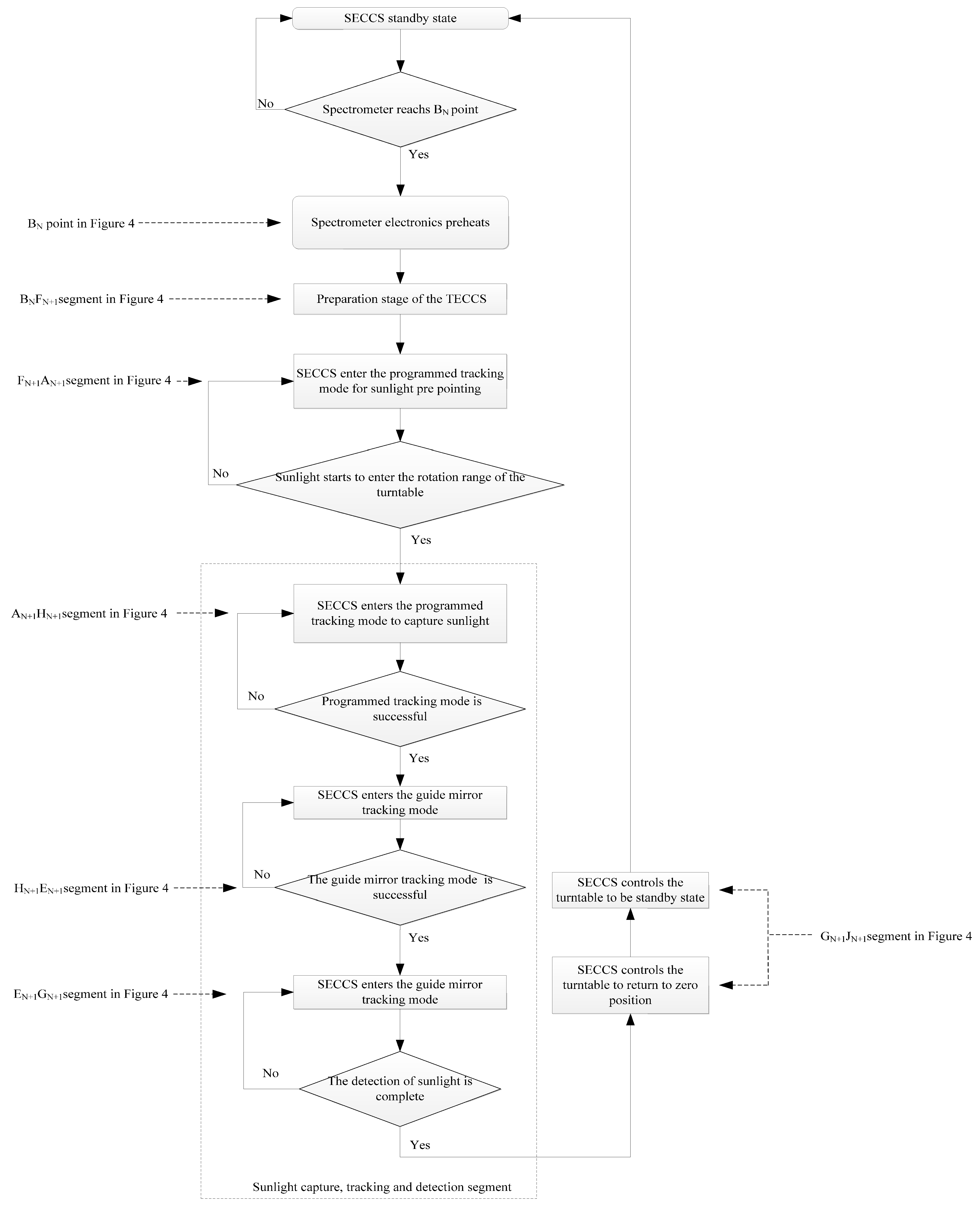
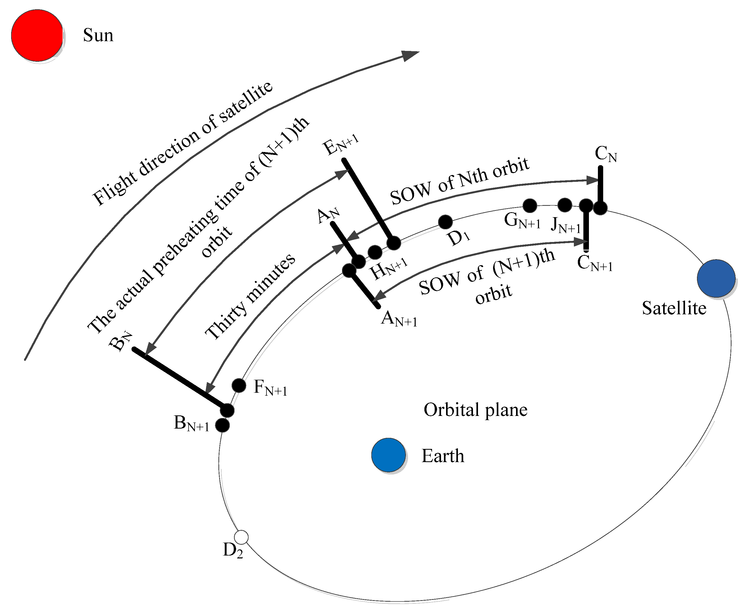
According to the orbit prediction function, the BN point of the Nth orbit is taken as the starting time of the spectrometer electronics preheating of the (N + 1)th orbit;
(2)
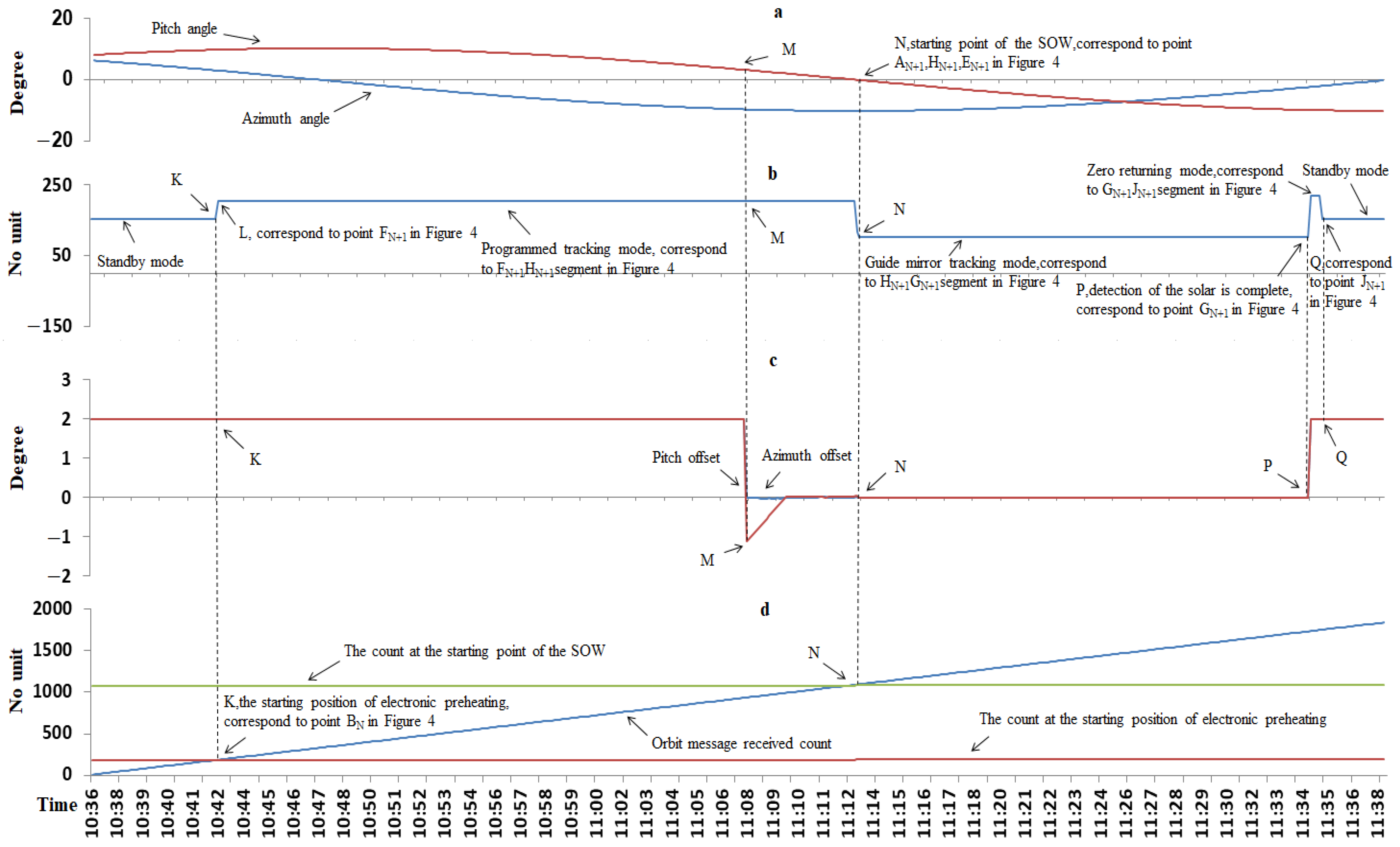
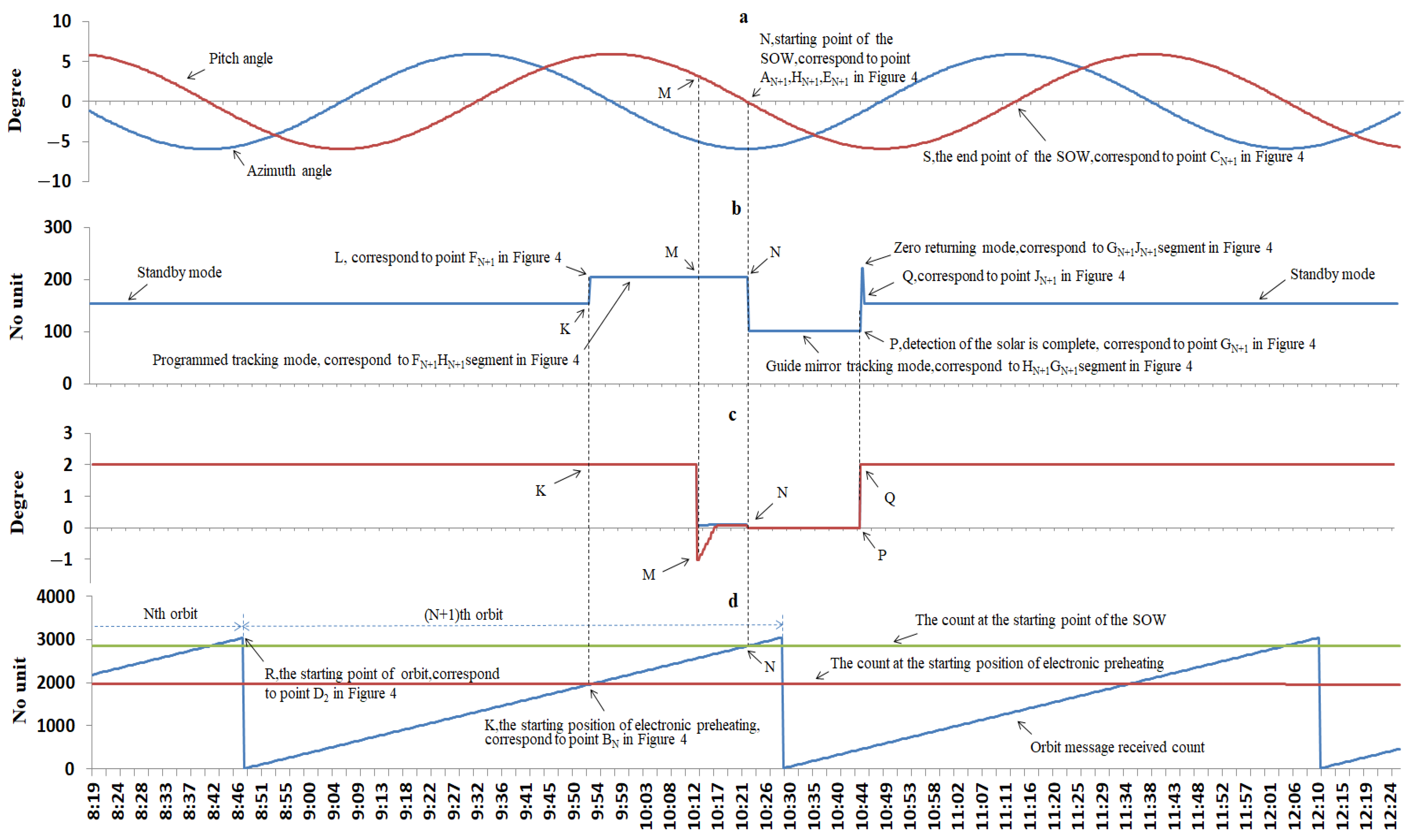
The preparation stage of the TECCS is approximately 3 s. In this stage, the electrical cabinet completes the software (The version number is 2.04) loading action from the standby state, corresponding to the BNFN+1 section in Figure 4;
(3)
After the TECCS is ready for tracking, the SECCS controls it to enter the programmed tracking mode for solar pre-pointing, corresponding to the FN+1AN+1 segment in Figure 4. At this time, the sunlight is outside the rotation range of the turntable. The TECCS controls the rotation of the turntable according to the received azimuth and pitch angles and uses the azimuth and pitch encoder angles to make a closed-loop control. At this time, no matter the relationship between the solar angle received by the TECCS and the angle quantity of the corresponding encoder, the SECCS does not switch the mode of the turntable. When the azimuth and pitch angles calculated by the SECCS are greater than or equal to the maximum rotation angle in the corresponding direction of the turntable, the extreme value of the rotation angle in the corresponding direction of the turntable is sent to the TECCS. At least one direction of the turntable azimuth and pitch waits for the sunlight to enter the turntable rotation range at the extreme range position. Compared with the turntable waiting for the sunlight to enter the field of view at the zero position, this mode realizes the purpose of rapid capture and tracking;
(4)
When the sunlight starts to enter the rotation range of the turntable (corresponding to the AN+1 point in Figure 4), the SECCS enters the programmed tracking mode to capture it. The TECCS still controls the rotation of the turntable according to the received azimuth angle and pitch angle and uses the azimuth and pitch encoder angles to make a closed-loop control. When the difference between the solar angle received by the TECCS and the corresponding encoder angle is less than 0.1° (corresponding to the HN+1 point in Figure 4), the programmed tracking mode is successful. The SECCS switches the operating mode of the turntable to the guide mirror tracking mode. As sunlight is at the edge of the rotating range of the turntable, the field of view of the guide mirror is a circular field with a radius of 1°. According to the error chain analysis of the SECCS, the sunlight enters the field of view of the guide mirror. This period corresponds to the AN+1HN+1 section in Figure 4;
(5)
In the guide mirror tracking mode, the TECCS controls the turntable azimuth and pitch motor rotation for closed-loop tracking according to the guide mirror offset. When the guide mirror azimuth and pitch offset are less than 0.1° (corresponding to the EN+1 point in Figure 4), the guide mirror tracking mode is successful;
(6)
When the guide mirror tracking mode is successful, the spectrometer starts to detect sunlight until the end of detection. This period corresponds to the EN+1GN+1 segment in Figure 4;
(7)
When the detection of sunlight is complete, the SECCS controls the turntable to return it to the zero position and enter it into the standby state. This period corresponds to the GN+1JN+1 section in Figure 4.
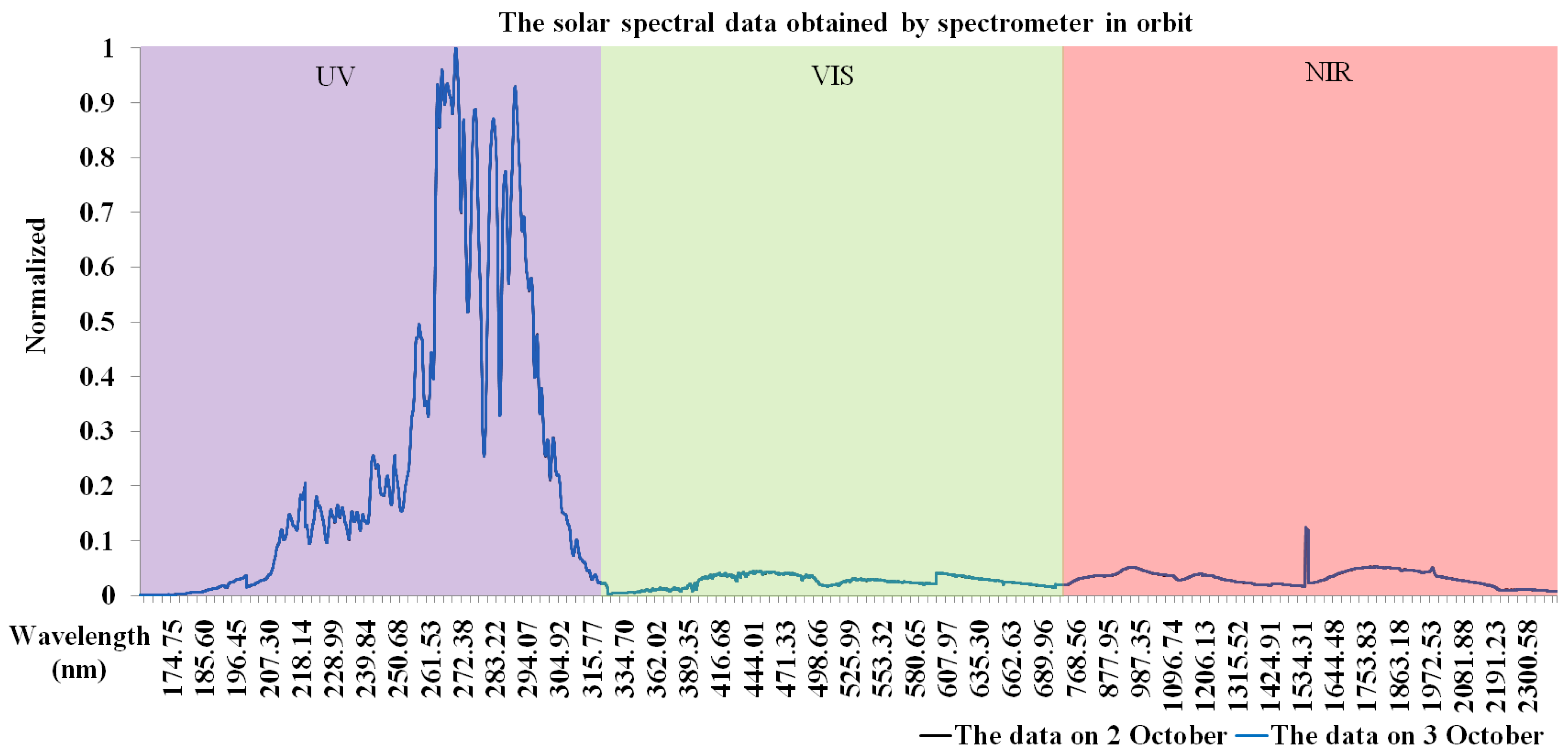
Figure 7. The SECCS’s function of a turntable control flow for the fast tracking of sunlight.
Remotesensing 15 03288 g007
In step (1)~step (7), the SECCS completes the process of solar capture, tracking, and detection. In steps (3) and (4), the purpose of the SECCS to track solar activity quickly is achieved.

3. Results

The spectrometer conducted orbit prediction experiments on the Earth’s surface in July 2020 and January 2021, respectively. The simulation experiment aimed to achieve orbit simulation solar tracking on the ground using a prediction function, as well as solar capture and SECCS tracking. Therefore, two-orbit simulation experiments measured on the ground were shown. The simulation experiment of the SECCS’s orbit prediction principle on the ground is shown in Figure 8. The light source emitted parallel light through the collimator and was fixed to simulate the sunlight. The front detector was fixed on the platform, which rotated according to the solar vector sent by the satellite simulator in orbit. The satellite simulator sent the data to the SECCS at the same time. The SECCS converted the data into the azimuth and pitch angles at the guide mirror coordinate system to control the rotation of the turntable. The solar irradiance spectrometer realized the orbit prediction, dynamic capture, and tracking of light sources by the turntable.
The results of the two solar tracking simulations and the SECCS orbit prediction function when on the Earth’s surface are shown in Figure 9 and Figure 10a–d. Viewed from the −Y-axis direction, the angle offset of the guide mirror in the +Z-axis range was negative, the angle offset of the −Z-axis range was positive, the angle offset of the −X-axis range was negative, and the angle offset of the +X-axis range was positive. When the orbit message count value was equal to the value at the beginning of preheating (point K of the curve (d) in Figure 9), that is, when the orbit message count value was equal to bN at the BN point in Figure 4, the solar detection mode started and the spectrometer electronics were powered on for preheating. At this time (point K of the curve (c) in Figure 9), the light source was located outside the field of view of the guide mirror, the azimuth and pitch offset had a fixed value of 2°, and the working mode of the TECCS (point K of the curve (b) in Figure 9) was on standby. As the preparation time of the TECCS is very short, the turntable working mode quickly switched from standby to the programmed tracking (pre-pointing) mode (point L of the curve (b) in Figure 9), corresponding to point FN+1 in Figure 4.
The programmed tracking mode continued to the starting point of the SOW (point N of the curve (a) in Figure 9). When the orbit message count value was equal to the value at the starting point of the SOW (point N of curve (d) in Figure 9), because the programmed tracking (solar capture) mode and the guide mirror tracking mode are completed in a very short time, the AN+1, HN+1, and EN+1 points in Figure 4 coincided as N points in Figure 9. The azimuth and pitch direction offsets of the guide mirror were all near 0° (point N of the curve (c) in Figure 9), and the turntable working mode was switched from programmed tracking to the guide mirror tracking mode (point N of the curve (b) in Figure 9), and the solar irradiance spectrometer started to detect the Sun’s activity. In the process of the programmed tracking mode, when the azimuth and pitch angles were –12.621° and 3.062° (point M of the curve (a) in Figure 9), the light source entered the edge of the field of view in the pitch direction of the guide mirror, and the azimuth direction entered the central field of view of the guide mirror. Therefore, the pitch offset of the guide mirror changed from 2° to −1.117°, and the azimuth offset changed from 2° to −0.034° (point M of the curve (c) in Figure 9).
When the spectrometer detection of sunlight was complete, the SECCS mode switched from the guide mirror tracking mode to the zero-returning mode (point P of the curve (b) in Figure 9). At this time, the light source was still in the central field of view of the guide mirror (point P of curve (c) in Figure 9). When the turntable returned to the zero position at azimuth and pitch detection, the SECCS mode switched from the zero-returning mode to the standby mode (point Q of the curve (b) in Figure 9). When the light source exited the field of view of the guide mirror, the azimuth and pitch offsets reached 2° (point Q of the curve (c) in Figure 9). The spectrometer performed complete orbit prediction, light source acquisition, and tracking and detection of the light process. The difference between Figure 9 and Figure 10 is in the specific angle values; Figure 10 is not described and explained repeatedly.
The spectrometer conducted solar capture, tracking, and detection in orbit on 2 October, 16 December, and 1 October 2021. Results of the solar tracking and the SECCS orbit prediction function in orbit for given dates (2 October, 16 December, and 1 October, as an example) are shown in Figure 11, Figure 12 and Figure 13. The key nodes of the electronics system preheating start time, the SECCS mode of turntable control switching, and the detection start time and end time were consistent with the ground simulation experiment. The R point of curve (d) in Figure 11 and the point with the same characteristics as this point were the track starting points, corresponding to the D1 point in Figure 4. As the relative position relationship between the track starting point and the mode starting point BN changes in real time in a year (as shown in Figure 11), the solar track starting point R in curve (d) was consistent with the D2 point in Figure 4. The S point of the curve (a) in Figure 11 was the endpoint of the SOW of the orbit, corresponding to the CN+1 point in Figure 4. The difference between Figure 11, Figure 12 and Figure 13 is in the specific angle values; Figure 12 and Figure 13 are not described and explained repeatedly. It can be seen from Figure 11, Figure 12 and Figure 13 that the orbit prediction function, solar capture, and tracking function of the spectrometer were normal in orbit, and the purpose of rapid solar tracking was achieved. Under the guide mirror tracking mode, the absolute values of the azimuth and pitch offsets were less than 0.002°, meeting the index requirements of 0.1°. The process of software (The version number is 2.05) orbit prediction, solar capture, and tracking was consistent and independent of time. Therefore, datasets of three orbits are provided to prove the correctness of this function.
The solar spectral data obtained by the spectrometer in orbit, which were normalized to 1 on 2 October and 3 October, are shown in Figure 14, and the data for 1 October and 16 December are shown in Figure 15. It can be seen from the figure that the solar spectral data measured over four days in the UV, VIS, and NIR bands had a good consistency. Since the tracking accuracy and the hardware preheating time were only two aspects of obtaining stable solar remote sensing data, solar remote sensing data from four orbits were provided to demonstrate that the tracking accuracy and preheating time met the requirements.

4. Discussion

There are four key topics for discussion:
  • Determining the preheating time of the hardware: This aspect should be thoroughly researched by examining different preheating durations on the ground, which can provide valuable insights for optimizing the process.
  • Identifying optical components that contribute to the stability of the optic system: An investigation involving experts in optical design can identify and characterize specific components that significantly influence the stability of the optic system.
  • Designing the guide mirror with a larger field of view: It was designed as a circular field with a radius of more than 1°, such as 60°. The solar data can be captured when the spectrometer is in orbit, which can simplify the control process of the turntable.
  • Designing the turntable with a larger rotation range, such as with azimuth and pitch directions of ±35°: This aspect should make the SOW as long as the orbital period, which meets the conditions for tracking and detecting the Sun in the whole orbit.
Aspects to be further verified include the following:
  • The results obtained on the ground (Equation (6)) and in orbit (Equation (7)) cannot be adequately supported solely by simulating solar tracking data on the ground and solar tracking and detection in orbit due to the difference in the telemetry parameters’ timing between the two scenarios (8 s on the ground versus 32 s in orbit).
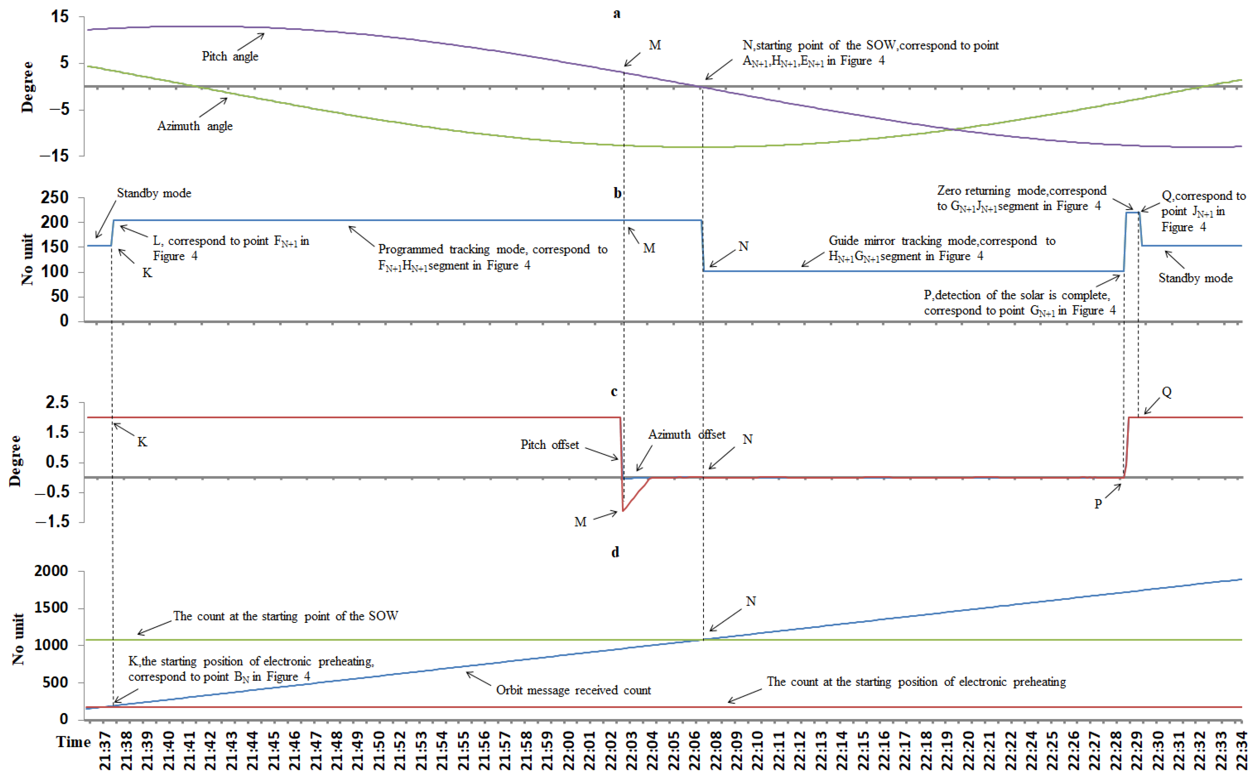
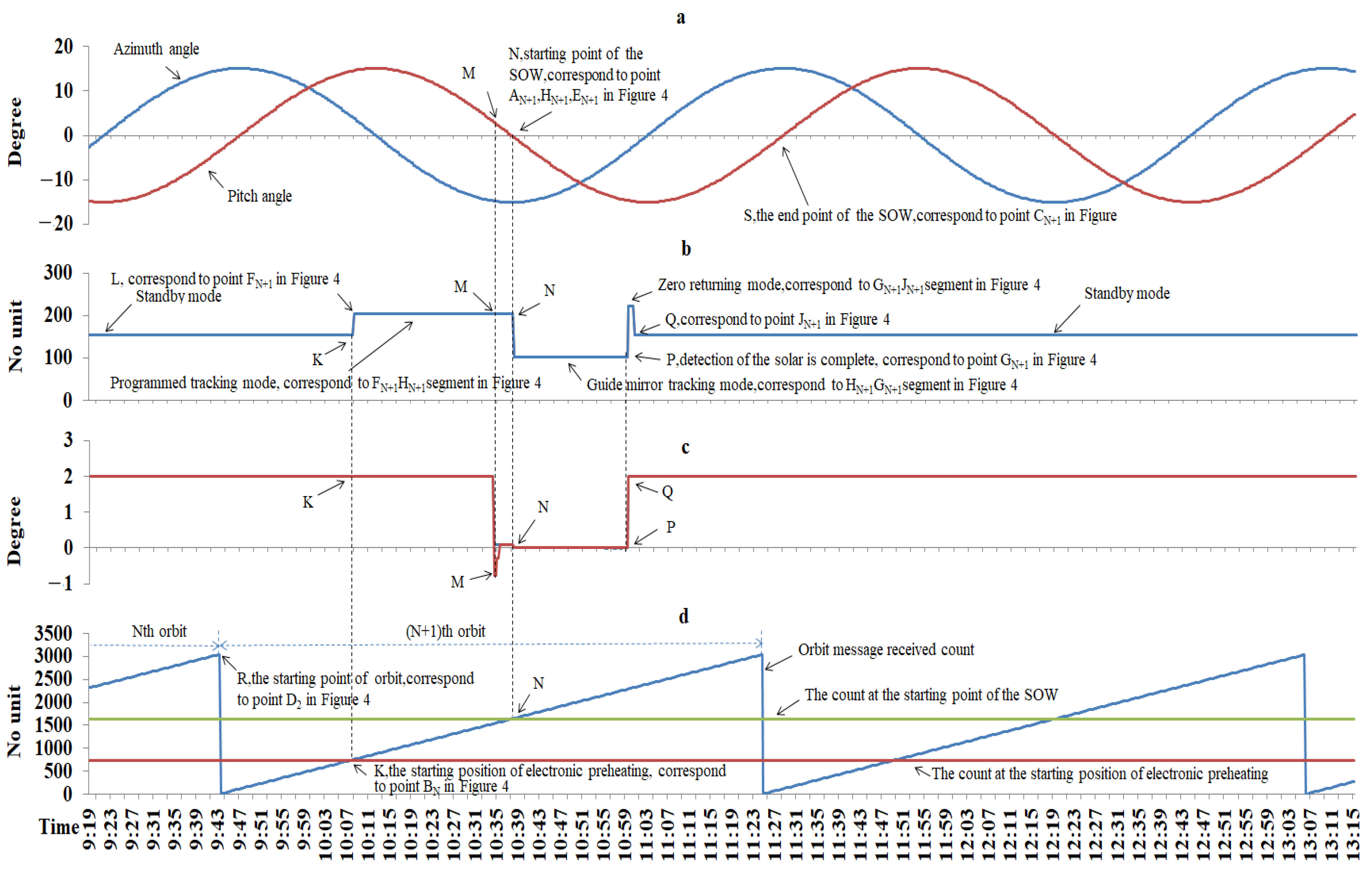
  • The results of the solar tracking simulation on the ground may not align perfectly with the MN section angle values of the curve (c) depicted in Figure 11, Figure 12 and Figure 13. This discrepancy can be attributed to the influence of the two-dimensional turntable’s balance on the ground, which differs from its weightless state in orbit.
  • The orbit prediction function of Aerospace Software is suitable for a Sun-synchronous orbit with any orbital inclination, but whether it is suitable for all kinds of orbits needs to be determined.
  • The solar remote sensing data should be compared with other international spectrometers to verify the accuracy of the measurement results.

5. Conclusions

The ground-simulated solar tracking experiment showed that the methods for orbit prediction and the fast tracking of solar activity are reasonable, feasible, simple, and reliable. The preheating time error of the payload electronics system was less than 1.3 s in theory and less than 8 s in the ground measurement, which meets the preheating time requirements and achieves the purpose of orbit prediction. The delay in the solar tracking success was less than 3.3 s in theory and less than 8 s in the actual measurement. The goal of fast tracking was achieved under the condition wherein the rotation range of the turntable was limited. The measured data show that the methods of orbit prediction and the fast tracking of the solar activity function were normally in orbit. The methods should be applied in different ε orbits.
The orbit prediction and fast-tracking solar methods make full use of the solar window period to carry out complete solar detection on the basis of meeting the electronics’ preheating time. At the same time, the tracking error of the turntable was less than 0.002°, which ensured that the instrument could obtain high-precision and stable solar spectral data. This can be summarized as follows:
  • The orbit prediction results were correct according to Figure 9 and Figure 10;
  • The fast-tracking solar method was effective according to Equations (6) and (7);
  • The mode switchings were the same in orbit according to the curve (b) in Figure 11, Figure 12 and Figure 13;
  • The Sun tracking accuracy met the system requirements according to the NP segment of curve (d) in Figure 11, Figure 12 and Figure 13, and the solar spectral detection results were stable in orbit according to Figure 14 and Figure 15.

6. Patents

We have applied for Chinese patents for both the orbit prediction method and the fast-tracking solar method, with the patent names of A Method for Predicting the Position of the Solar on the Solar Synchronous Orbit, and A Method for Fast Solar Capture and Tracking by Aerospace Software on the Solar Synchronous Orbit. The corresponding patent application numbers are 202111477431.3 and 202211344980.8. They are currently awaiting review by the China National Intellectual Property Administration.

Author Contributions

Conceptualization, Y.S.; methodology, Y.S.; software, Y.S.; validation, Y.S.; formal analysis, Y.S.; investigation, Y.S.; resources, Y.S.; data curation, X.Y., Z.L., Y.H., B.L., G.L., X.G. and J.L.; writing—original draft preparation, Y.S.; writing—review and editing, Y.S. All authors have read and agreed to the published version of the manuscript.

Funding

This research was funded by National Natural Science Foundation of China (No. 62205330) and National key research and development program of China (No. 2022YFB3903202).

Institutional Review Board Statement

Not applicable.

Informed Consent Statement

Not applicable.

Data Availability Statement

The data is unavailable due to privacy or ethical restrictions.

Conflicts of Interest

The authors declare no conflict of interest.

References

  1. Ding, Y.H. Effect of Solar Activity on Earth’s Climate and Weather. Meteorol. Mon. 2019, 45, 297–304. [Google Scholar]
  2. Kagata, H.; Yamamura, K. Special Feature: Global Climate Change and the Dynamics of Biological Communities—Preface. Popul. Ecol. 2006, 48, 3–4. [Google Scholar] [CrossRef]
  3. Lin, W.; Lu, E. Annual and Seasonal Global Solar-Radiation Climates in YunNan, China. Energy Convers. Manag. 1992, 33, 1021–1029. [Google Scholar]
  4. Yilmaz, E. A Systematic Study on the Monthly Mean Global Solar Radiation between Latitudes 65S and 65N. Energy Sources Part A Recovery Util. Environ. Eff. 2011, 33, 434–439. [Google Scholar] [CrossRef]
  5. Ricke, K.; Morgan, G.; Allen, M. Regional Climate Response to Solar-radiation Management. Nat. Geosci. 2010, 3, 537–541. [Google Scholar] [CrossRef]
  6. Wen, G.; Cahalan, R.; Rind, D.; Jonas, J.; Pilewskie, P.; Harder, J. Spectral Solar UV Radiation and Its Variability and Climate Responses. In Proceedings of the International Radiation Symposium on Radiation Processes in the Atmosphere and Ocean (IRS), Berlin, Germany, 6–10 August 2012; Volume 1531, pp. 788–791. [Google Scholar]
  7. Kambezidis, H. The Solar Radiation Climate of Athens: Variations and Tendencies in the Period 1992–2017, the Brightening Era. Sol. Energy 2018, 173, 328–347. [Google Scholar] [CrossRef]
  8. Matuszko, D. Long-term Variability in Solar Radiation in Krakow Based on Measurements of Sunshine Duration. Int. J. Climatol. 2014, 34, 228–234. [Google Scholar] [CrossRef]
  9. Pasini, A.; Triacca, U.; Attanasio, A. Evidence of Recent Causal Decoupling between Solar Radiation and Global Temperature. Environ. Res. Lett. 2012, 7, 034020. [Google Scholar] [CrossRef]
  10. Madhlopa, A. Solar Radiation Climate in Malawi. Sol. Energy 2006, 80, 1055–1057. [Google Scholar] [CrossRef]
  11. Mitchell, J.; Nolfo, G.; Hill, M.; Christian, E.; McComas, D.; Schwadron, N.; Wiedenbeck, M.; Bale, S.; Case, A.; Cohen, C.; et al. Small Electron Events Observed by Parker Solar Probe/ISeIS during Encounter 2. Astrophys. J. 2020, 902, 20. [Google Scholar] [CrossRef]
  12. Zhao, L.L.; Zank, G.; Hu, Q.; Telloni, D.; Chen, Y.; Adhikari, L.; Nakanotani, M.; Kasper, J.; Huang, J.; Bale, S.; et al. Detection of small magnetic flux ropes from the third and fourth Parker Solar Probe encounters. Astron. Astrophys. 2021, 650, A12. [Google Scholar] [CrossRef]
  13. Sakshee, S.; Riddhi, B.; Supratik, B. MHD-scale anisotropy in solar wind turbulence near the Sun using Parker solar probe data. Mon. Not. R. Astron. Soc. 2022, 514, 1282–1288. [Google Scholar] [CrossRef]
  14. Sebastian, A.; Acedo, L.; Morano, J. An orbital model for the Parker Solar Probe mission: Classical vs relativistic effects. Adv. Space Res. 2022, 70, 842–853. [Google Scholar] [CrossRef]
  15. Alberti, T.; Benella, S.; Benzi, R. Reconciling Parker Solar Probe Observations and Magnetohydrodynamic Theory. Astrophys. J. Lett. 2022, 940, 1. [Google Scholar] [CrossRef]
  16. Raouafifi, N.; Matteini, L.; Squire, J.; Badman, S.; Velli, M.; Klein, K.; Chen, C.; Matthaeu, W.; Szabo, A.; Linton, M.; et al. Parker Solar Probe: Four Years of Discoveries at Solar Cycle Minimum. Space Sci. Rev. 2023, 219, 8. [Google Scholar] [CrossRef]
  17. Thuillier, G.; Frohlich, C.; Schmidtke, G. Spectral and total solar irradiance measurements on board the International Space Station. In Proceedings of the 2nd European Symposium on Utilisation of the International Space Station, Noordwijk, The Netherlands, 16–18 November 1998; Volume 433, pp. 605–611. [Google Scholar]
  18. Schmidtke, G.; Frohlich, C.; Thuillier, G. ISS-SOLAR: Total (TSI) and Spectral (SSI) Irradiance Measurements. Adv. Space Res. 2006, 37, 255–264. [Google Scholar] [CrossRef]
  19. Thuillier, G.; Foujols, T.; Bolsee, D.; Gillotay, D.; Herse, M.; Peetermans, W.; Decuyper, W.; Mandel, H.; Sperfeld, P.; Pape, S. SOLAR/SOLSPEC: Scientific Objectives, Instrument Performance and Its Absolute Calibration Using a Blackbody as Primary Standard Source. Sol. Phys. 2009, 257, 185–213. [Google Scholar] [CrossRef]
  20. Weber, M. Comment on the Article by Thuillier et al. “The Infrared Solar Spectrum Measured by the SOLSPEC Spectrometer onboard the International Space Station”. Sol. Phys. 2015, 290, 1601–1605. [Google Scholar] [CrossRef]
  21. Wienhold, F.; Anders, J.; Galuska, B.; Klocke, U.; Knothe, M.; Riedel, W.; Schmidtke, G.; Singler, R.; Ulmer, U.; Wolf, H. The solar package on ISS: SOL-ACES. In Proceedings of the 2nd TIGER Symposia A Program for Thermospheric-Iono Spheric Geospheric Research, St. Petersburg, Russia, 9–10 June 1999; Volume 25, pp. 473–476. [Google Scholar]
  22. Vourlidas, A. Ly alpha science from the LST aboard the ASO-S mission. Res. Astron. Astrophys. 2019, 19, 11. [Google Scholar] [CrossRef]
  23. Gan, W.Q. Progress Report on ASO-S. Chin. J. Space Sci. 2022, 42, 565–567. [Google Scholar] [CrossRef]
  24. Gan, W.Q. Status of the Advanced Space-based Solar Observatory. Chin. J. Space Sci. 2020, 40, 704–706. [Google Scholar]
  25. Huang, Y.Y.; Ma, T.; Zhang, Y.Q.; Zhang, Y.; Zhang, Z. Calibration of the Detector Units of the Spectrometer of the Hard X-ray Imager Payload Onboard the ASO-S Mission. Acta Astron. Sin. 2020, 61, 42. [Google Scholar]
  26. Fang, C.; Li, C. Introduction to the Chinese Halpha Solar Explorer (CHASE) Mission. Chin. J. Space Sci. 2022, 42, 546–549. [Google Scholar] [CrossRef]
  27. Ye, X.; Yi, X.; Lin, C.; Fang, W.; Wang, K.; Xia, Z.; Ji, Z.; Zheng, Y.; Sun, D.; Quan, J. Instrument Development: Chinese Radiometric 122 Benchmark of Reflected Solar Band Based on Space Cryogenic Absolute Radiometer. Remote Sens. 2020, 12, 2856. [Google Scholar] [CrossRef]
  28. Yang, D.; Fang, W.; Ye, X.; Song, B. High Precision Sun–tracking of Spaceborne Solar Irradiance Monitor. Opt. Precis. Eng. 2014, 22, 2483–2490. [Google Scholar] [CrossRef]
  29. Li, Z.; Wang, S.; Huang, Y.; Lin, G.; Shao, Y.; Yu, M. High-Precision and Short-Time Solar Forecasting by Spaceborne Solar Irradiance Spectrometer. Acta Opt. Sin. 2019, 39, 1–5. [Google Scholar]
  30. Shao, Y.; Li, Z.; Yang, X.; Huang, Y.; Li, B.; Lin, G.; Li, J. Methods of Analyzing the Error and Rectifying the Calibration of a Solar Tracking System for High-Precision Solar Tracking in Orbit. Remote Sens. 2023, 15, 2213. [Google Scholar] [CrossRef]
  31. Liu, G.; Hu, J. Design of Communication Stream for the 1553B Bus. J. Beijing Inst. Technol. 2003, 23, 301–304. [Google Scholar]
  32. Kanchana, G.; Kumar, M.S. Avionics system network with MIL-STD 1553B bus. J. Inst. Electron. Telecommun. Eng. 1995, 41, 291–295. [Google Scholar] [CrossRef]
  33. Sabnis, A.; Hotkar, V.; Vanathy, B.; Jacob, A. 1553B Communication Using DSP Based Digital Controller. In Proceedings of the International Conference on Control, Instrumentation, Energy and Communication (CIEC), Kolkata, India, 31 January–2 February 2014; pp. 485–489. [Google Scholar]
  34. Rao, D.; Raja, A.; Karthikeyan, R.; Pal, K.; Tharun, S.; Priya, B. Design and Implementation of 1553B Bus Controller on FPGA. In Proceedings of the 3rd International Conference on Computing Methodologies and Communication (ICCMC), Erode, India, 27–29 March 2019; IEEE: New York, NY, USA, 2019; pp. 418–421. [Google Scholar]
  35. Burgess, R. RS422 and Beyond. Electron. Eng. 1981, 53, 81. [Google Scholar]
  36. Zhang, Y.; Cheng, J.; Su, J.; Zheng, L.; Qiu, X.; Shang, W. Time-domain resonant characteristics between the disturbances and the 129 RS422 communication signals in Tesla pulse driver, and analysis on the caused RS422 communication interference. IET Sci. Meas. Technol. 2020, 14, 905–913. [Google Scholar] [CrossRef]
  37. Shi, L.; Guo, B. RS485/422 Solution in Embedded Access Control System. In Proceedings of the 2nd International Conference on Biomedical Engineering and Informatics (BMEI), Tianjin, China, 17–19 October 2009; pp. 2094–2097. [Google Scholar]
Figure 1. (a) The composition of the spectrometer and satellite and the spectrometer coordinate systems. (b) Orbital coordinate system and parameter, with the satellite moving around the Earth. (c) The position relationship between the Sun, the Earth, and the satellite and the position of the front detector on the satellite.
Remotesensing 15 03288 g001aRemotesensing 15 03288 g001b
Figure 2. (a) The internal connection relation of the spectrometer and the connection relation with the satellite. (b) The satellite and the spectrometer’s software (The version number is 2.05) data flow of the turntable control.
Remotesensing 15 03288 g002
Figure 3. (a) Schematic drawing of the solar cone, azimuth, and pitch angle in the guide mirror coordinate system. (b) Yearly variation of the solar cone angle with time.
Remotesensing 15 03288 g003
Figure 4. Orbit prediction of the (N + 1)th according to the Nth orbit and the actual preheating time of the (N + 1)th orbit.
Remotesensing 15 03288 g004
Figure 5. Orbit message counts at the starting point of the SOW in orbit for a day.
Remotesensing 15 03288 g005
Figure 6. Relationship of the five CSs involved in the calculation of the solar angle.
Remotesensing 15 03288 g006
Figure 8. The simulation experiment of the SECCS’s orbit prediction principle on the ground.
Remotesensing 15 03288 g008
Figure 9. Results of the first solar tracking simulation and the SECCS orbit prediction function when on the Earth’s surface. (a) Azimuth and pitch angles of solar at guide mirror coordinate system. (b) The work mode of SECCS to control turntable. (c) The azimuth and pitch offsets of the guide mirror. (d) The orbit message received count.
Remotesensing 15 03288 g009
Figure 10. Results of the second solar tracking simulation and the SECCS orbit prediction function when on the Earth’s surface. (a) Azimuth and pitch angles of solar at guide mirror coordinate system. (b) The work mode of SECCS to control turntable. (c) The azimuth and pitch offsets of the guide mirror. (d) The orbit message received count.
Remotesensing 15 03288 g010
Figure 11. Results of the solar tracking and the SECCS orbit prediction function in orbit for a given date (2 October, as an example). (a) Azimuth and pitch angles of solar at guide mirror coordinate system. (b) The work mode of SECCS to control turntable. (c) The azimuth and pitch offsets of the guide mirror. (d) The orbit message received count.
Remotesensing 15 03288 g011
Figure 12. Results of the solar tracking and the SECCS orbit prediction function in orbit for a given date (16 December, as an example). (a) Azimuth and pitch angles of solar at guide mirror coordinate system. (b) The work mode of SECCS to control turntable. (c) The azimuth and pitch offsets of the guide mirror. (d) The orbit message received count.
Remotesensing 15 03288 g012
Figure 13. Results of the solar tracking and the SECCS orbit prediction function in orbit for a given date (1 October, as an example). (a) Azimuth and pitch angles of solar at guide mirror coordinate system. (b) The work mode of SECCS to control turntable. (c) The azimuth and pitch offsets of the guide mirror. (d) The orbit message received count.
Remotesensing 15 03288 g013
Figure 14. The solar spectral data obtained by the spectrometer in ultraviolet (UV), visible (VIS), and near-infrared (NIR) in orbit for a given date (2 October and 3 October, as an example).
Remotesensing 15 03288 g014
Figure 15. The solar spectral data obtained by the spectrometer in ultraviolet (UV), visible (VIS), and near-infrared (NIR) in orbit for a given date (1 October and 16 December, as an example).
Remotesensing 15 03288 g015
Disclaimer/Publisher’s Note: The statements, opinions and data contained in all publications are solely those of the individual author(s) and contributor(s) and not of MDPI and/or the editor(s). MDPI and/or the editor(s) disclaim responsibility for any injury to people or property resulting from any ideas, methods, instructions or products referred to in the content.

