
Region-Based Sea Ice Mapping Using Compact Polarimetric Synthetic Aperture Radar Imagery with Learned Features and Contextual Information

Abstract
1. Introduction
2. Background
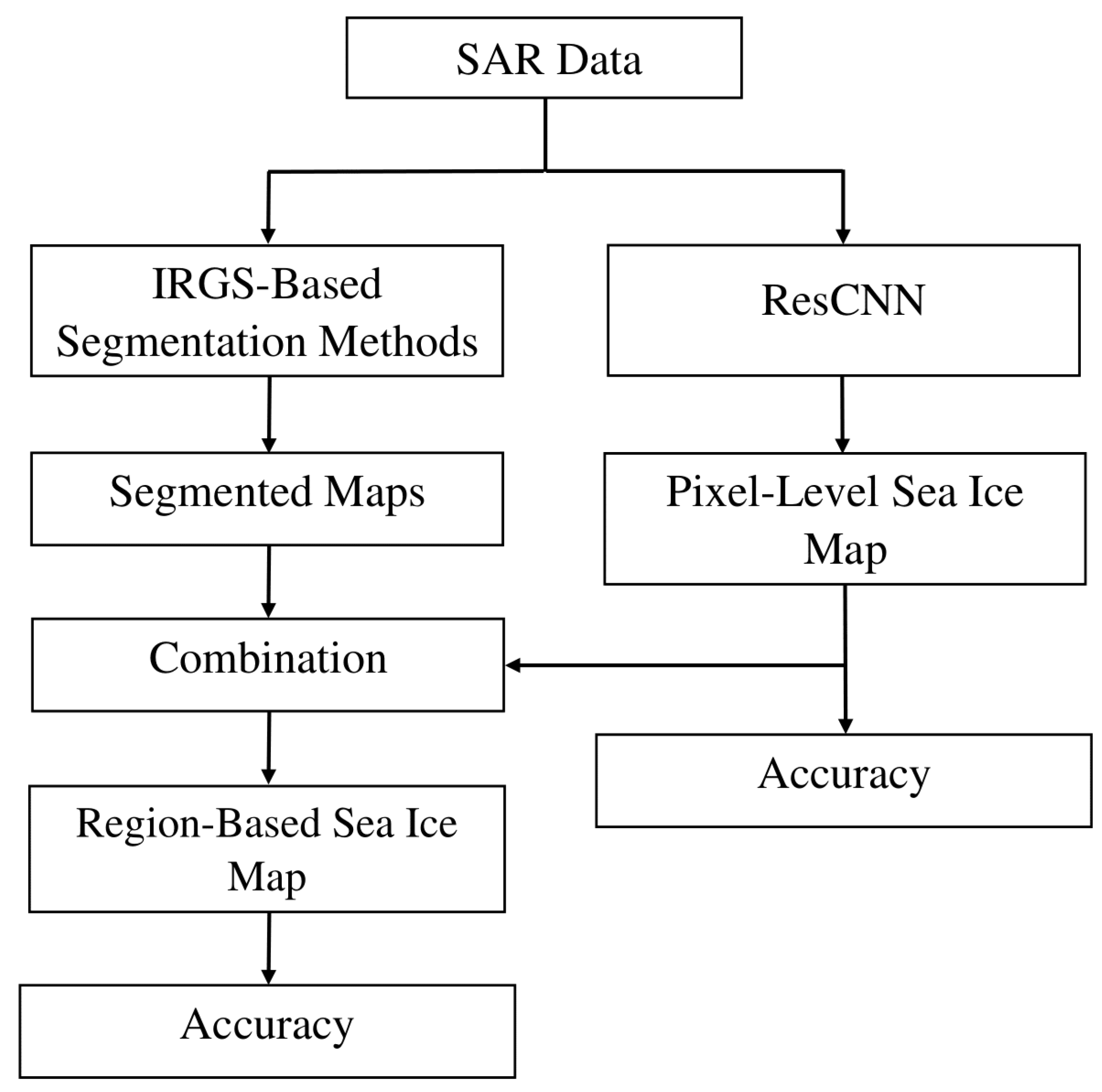
3. Methodology
- The various SAR modes (Section 3.1) each used as source imagery are CP, DP, RQP, and QP as input to the region-based segmentation and pixel-level classification methods;
- A ResCNN model is used to generate the pixel-level sea ice maps by using learned features from each of the modes (Section 3.2);
- Unsupervised segmentation algorithms, which are mode dependent, are used to generate homogeneous, contiguous regions with accurate class boundaries (Section 3.3);
- The segmented and pixel-level classified images are combined by a region-based majority voting approach (Section 3.4).
3.1. SAR Data
3.1.1. QP SAR Data
3.1.2. Synthesized CP SAR Data
3.1.3. Reconstructed QP SAR Data
3.1.4. DP SAR Data
3.2. Sea Ice Classification Using ResCNN Model
3.3. Obtaining Homogeneous Edge-Preserved Regions
3.4. Combining Pixel-Based Classification and Region-Based Segmentation
4. Experiments
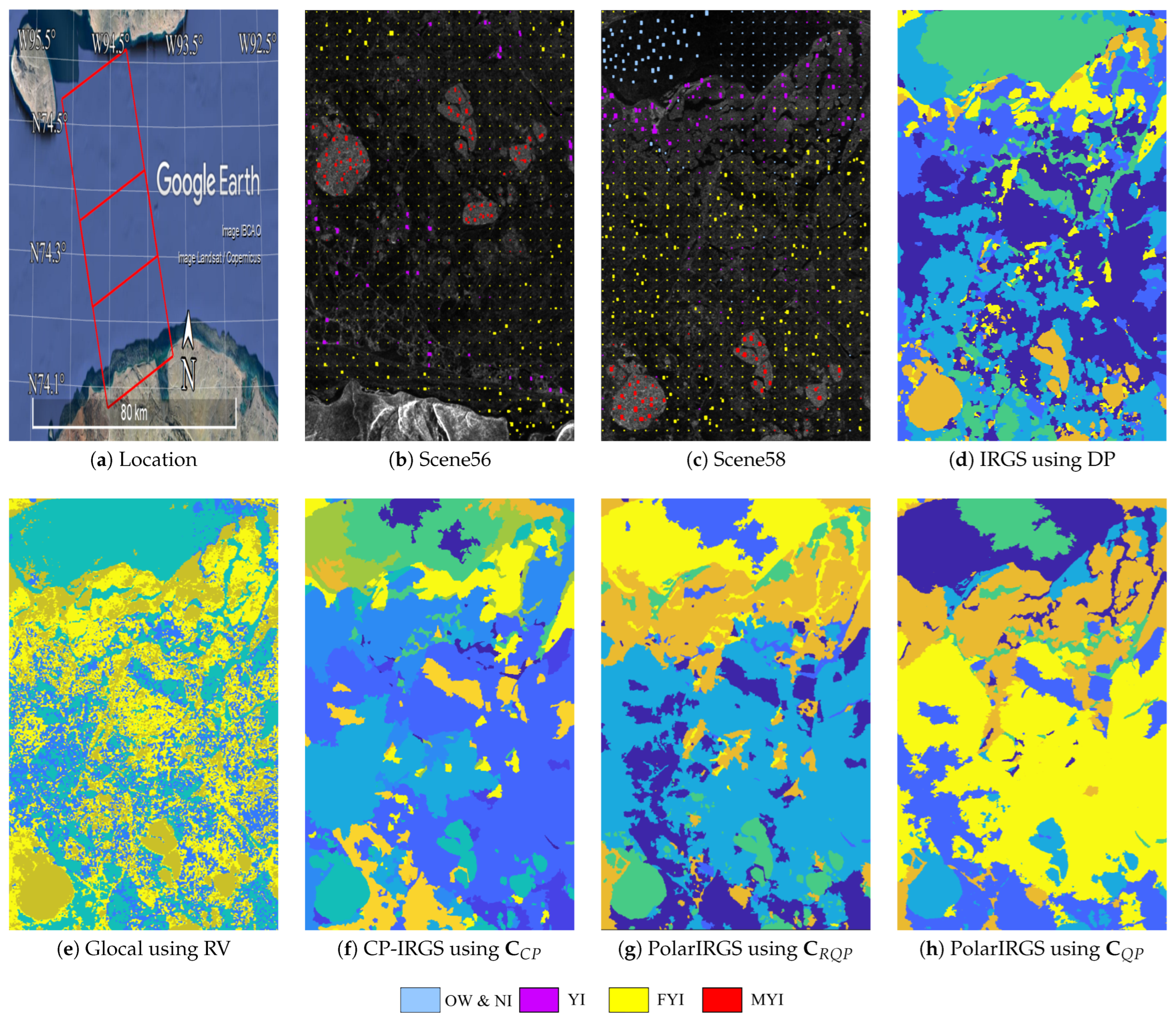
4.1. Study Area and Dataset
4.2. Training and Testing Data
4.3. Model Settings
4.4. Comparing CP, DP, RQP, and QP Modes
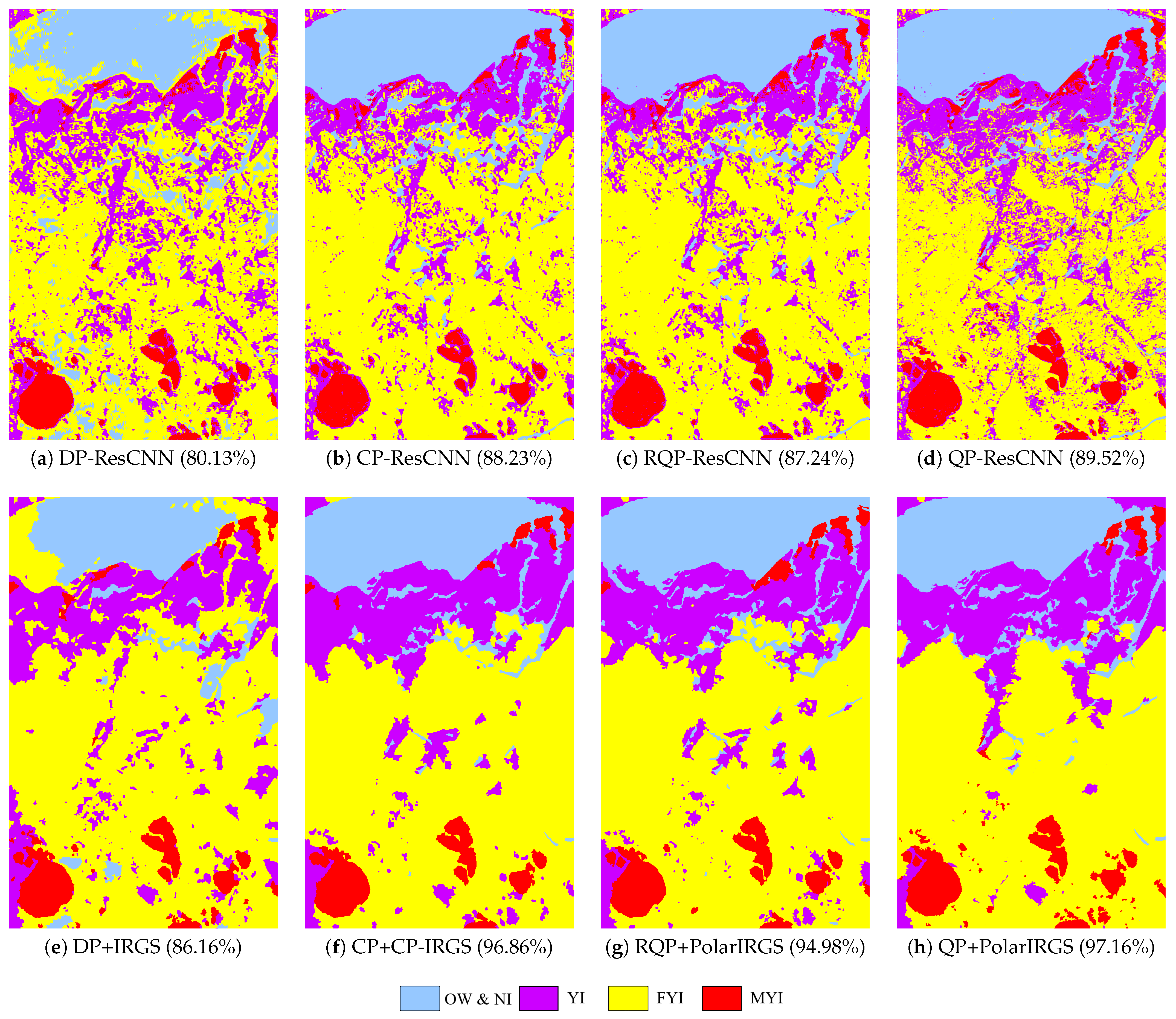
4.5. Performance Comparison of the Proposed Methodology with the Baselines
5. Conclusions
Author Contributions
Funding
Data Availability Statement
Conflicts of Interest
References
- Barber, D.G. Microwave remote sensing, sea ice and Arctic climate. Phys. Can 2005, 61, 105–111. [Google Scholar]
- Ghanbari, M.; Clausi, D.A.; Xu, L.; Jiang, M. Contextual Classification of Sea-Ice Types Using Compact Polarimetric SAR Data. IEEE Trans. Geosci. Remote Sens. 2019, 57, 7476–7491. [Google Scholar] [CrossRef]
- Charbonneau, F.J.; Arkett, M.; Brisco, B.; Buckley, J.; Chen, H.; Goodenough, D.G.; Liu, C.; McNarin, H.; Poitevin, J.; Shang, J.; et al. Meeting Canadian user needs with the RADARSAT Constellation Mission’s compact polarimetry mode: A summary assessment. Nat. Resour. Can. Ott. Geomat. Can. Open File. 2017, 34, 78. [Google Scholar]
- Raney, R.K. Hybrid-polarity SAR architecture. IEEE Trans. Geosci. Remote Sens. 2007, 45, 3397–3404. [Google Scholar] [CrossRef]
- Dabboor, M.; Geldsetzer, T. Towards sea ice classification using simulated RADARSAT Constellation Mission compact polarimetric SAR imagery. Remote Sens. Environ. 2014, 140, 189–195. [Google Scholar] [CrossRef]
- Singha, S.; Ressel, R. Arctic sea ice characterization using RISAT-1 compact-pol SAR imagery and feature evaluation: A case study over Northeast Greenland. IEEE J. Sel. Top. Appl. Earth Obs. Remote Sens. 2017, 10, 3504–3514. [Google Scholar] [CrossRef]
- Espeseth, M.M.; Brekke, C.; Anfinsen, S.N. Hybrid-polarity and reconstruction methods for sea ice with L- and C-band SAR. IEEE Geosci. Remote Sens. Lett. 2016, 13, 467–471. [Google Scholar] [CrossRef]
- Geldsetzer, J.; Arkett, M.; Zagon, T.; Charbonneau, F. All-season compact-polarimetry C-band SAR observations of sea ice. Can. J. Remote Sens. 2015, 41, 485–504. [Google Scholar] [CrossRef]
- Li, H.; William, P. Sea ice characterization and classification using hybrid polarimetry SAR. IEEE J. Sel. Top. Appl. Earth Obs. Remote Sens. 2016, 9, 4998–5010. [Google Scholar] [CrossRef]
- Zhang, X.; Zhang, J.; Liu, M.; Meng, J. Assessment of C-band compact polarimetry SAR for sea ice classification. Acta Oceanol. Sin. 2016, 35, 79–88. [Google Scholar] [CrossRef]
- Dabboor, M.; Montpetit, B.; Howell, S. Assessment of the high resolution SAR mode of the RADARSAT Constellation Mission for first year ice and multiyear ice characterization. Remote Sens. 2018, 10, 594. [Google Scholar] [CrossRef]
- Nasonova, S.; Scharien, R.K.; Geldsetzer, T.; Howell, S.; Power, D. Optimal compact polarimetric parameters and texture features for discriminating sea ice types during winter and advanced melt. Can. J. Remote Sens. 2018, 44, 390–411. [Google Scholar] [CrossRef]
- Song, W.; Li, M.; Gao, W.; Huang, D.; Zhenling, M.; Liotta, A.; Perra, C. Automatic sea-ice classification of SAR images based on spatial and temporal features learning. IEEE Trans. Geosci. Remote Sens. 2021, 59, 9887–9901. [Google Scholar] [CrossRef]
- Liu, W.; Wang, W.; Zhao, Q.; Shen, X.; Konan, M. A new feature selection method based on a validity index of feature subset. IEEE Trans. Geosci. Remote Sens. 2017, 92, 1–8. [Google Scholar] [CrossRef]
- Wang, L.; Scott, A.K.; Xu, L.; Clausi, D.A. Sea ice concentration estimation during melt from dual-pol SAR scenes using deep convolutional neural networks: A case study. IEEE Trans. Geosci. Remote Sens. 2016, 54, 4524–4533. [Google Scholar] [CrossRef]
- Lyu, H.; Huang, W.; Mahdianpari, M. Eastern Arctic Sea Ice Sensing: First Results from the RADARSAT Constellation Mission Data. Remote Sens. 2022, 14, 1165. [Google Scholar] [CrossRef]
- Xu, Y.; Scott, A.K. Sea ice and open water classification of SAR imagery using CNN-based transfer learning. In Proceedings of the 2017 IEEE International Geoscience and Remote Sensing Symposium (IGARSS), Fort Worth, TX, USA, 23–28 July 2017; pp. 3262–3265. [Google Scholar]
- Ren, Y.; Li, X.; Yang, X.; Xu, H. Development of a Dual-Attention U-Net Model for Sea Ice and Open Water Classification on SAR Images. IEEE Geosci. Remote Sens. Lett. 2022, 19, 1–5. [Google Scholar] [CrossRef]
- Khaleghian, S.; Ullah, H.; Kræmer, T.; Hughes, N.; Eltoft, T.; Marinoni, A. Sea ice classification of SAR imagery based on convolution neural networks. Remote Sens. 2021, 13, 1734. [Google Scholar] [CrossRef]
- Han, Y.; Liu, Y.; Hong, Z.; Zhang, Y.; Yang, S.; Wang, J. Sea ice image classification based on heterogeneous data fusion and deep learning. Remote Sens. 2021, 13, 592. [Google Scholar] [CrossRef]
- Huang, Y.; Ren, Y.; Li, X. Classifying Sea Ice Types from SAR Images Using a U-Net-Based Deep Learning Model. In Proceedings of the 2021 IEEE International Geoscience and Remote Sensing Symposium (IGARSS), Brussels, Belgium, 11–16 July 2021; pp. 3502–3505. [Google Scholar]
- Gao, Y.; Gao, F.; Dong, J.; Wang, S. Transferred deep learning for sea ice change detection from synthetic-aperture radar images. IEEE Geosci. Remote Sens. Lett. 2019, 16, 1655–1659. [Google Scholar] [CrossRef]
- Bentes, C.; Frost, A.; Velotto, D.; Tings, B. Ship-iceberg discrimination with convolutional neural networks in high resolution SAR images. In Proceedings of the EUSAR 2016: 11th European Conference on Synthetic Aperture Radar, Hamburg, Germany, 6–9 June 2016; pp. 1–4. [Google Scholar]
- He, K.; Zhang, X.; Ren, S.; Sun, J. Deep residual learning for image recognition. In Proceedings of the IEEE Conference on Computer Vision and Pattern Recognition (CVPR), Las Vegas, NV, USA, 27–30 June 2016; pp. 770–778. [Google Scholar]
- Guo, S.; Tian, Y.; Li, Y.; Chen, S.; Hong, W. Unsupervised classification based on H/alpha decomposition and Wishart classifier for compact polarimetric SAR. In Proceedings of the 2015 IEEE International Geoscience and Remote Sensing Symposium (IGARSS), Milan, Italy, 26–31 July 2015; pp. 1614–1617. [Google Scholar]
- Khedama, R.; Belhadj-Aissaa, A. Contextual classification of remotely sensed data using MAP approach and MRF. ISPRS J. Photogramm. Remote Sens. 2004, 35, 11–16. [Google Scholar]
- Ghanbari, M.; Clausi, D.A.; Xu, L. CP-IRGS: A Region-Based Segmentation of Multilook Complex Compact Polarimetric SAR Data. IEEE J. Sel. Top. Appl. Earth Obs. Remote Sens. 2021, 14, 6559–6571. [Google Scholar] [CrossRef]
- Leigh, S.; Wang, Z.; Clausi, D.A. Automated ice–water classification using dual polarization SAR satellite imagery. IEEE Trans. Geosci. Remote Sens. 2013, 52, 5529–5539. [Google Scholar] [CrossRef]
- Raney, R.K.; Cahill, J.; Patterson, G.W.; Bussey, D.J. The m-chi decomposition of hybrid dual-polarimetric radar data with application to lunar craters. J. Geophys. Res. Planets 2012, 117. [Google Scholar] [CrossRef]
- Charbonneau, F.J.; Brisco, B.; Raney, R.K.; McNairn, H.; Liu, C.; Vachon, P.W.; Shang, J.; DeAbreu, R.; Champagne, C.; Geldsetzer, A.M.; et al. Compact polarimetry overview and applications assessment. Can. J. Remote Sens. 2010, 36, S298–S315. [Google Scholar] [CrossRef]
- Espeseth, M.M.; Brekke, C.; Johansson, A.M. Assessment of RISAT-1 and RADARSAT-2 for sea ice observations from a hybrid-polarity perspective. Remote Sens. 2017, 9, 1088. [Google Scholar] [CrossRef]
- Souyris, J.-C.; Imbo, P.; Fjortoft, R.; Mingot, S.; Lee, J.S. Compact polarimetry based on symmetry properties of geophysical media: The π/4 mode. IEEE Trans. Geosci. Remote Sens. 2005, 43, 634–646. [Google Scholar] [CrossRef]
- Nord, M.E.; Ainsworth, T.L.; Lee, J.; Stacy, N.J. Comparison of compact polarimetric synthetic aperture radar modes. IEEE Trans. Geosci. Remote Sens. 2008, 47, 174–188. [Google Scholar] [CrossRef]
- Ainsworth, T.L.; Kelly, J.P.; Lee, J.-S. Classification comparisons between dual-pol, compact polarimetric and quad-pol SAR imagery. ISPRS J. Photogramm. Remote Sens. 2009, 64, 464–471. [Google Scholar] [CrossRef]
- Goodfellow, I.; Bengio, Y.; Courville, A. Deep Learning; MIT Press: Cambridge, MA, USA, 2016; pp. 203–218, 277–282. ISBN 9780262337434. [Google Scholar]
- Bengio, Y.; Courville, A.; Vincent, P. Representation learning: A review and new perspectives. IEEE Trans. Pattern Anal. Mach. Intell. 2013, 35, 1798–1828. [Google Scholar] [CrossRef]
- Yu, Q.; Clausi, D.A. IRGS: Image segmentation using edge penalties and region growing. IEEE Trans. Pattern Anal. Mach. Intell. 2008, 30, 2126–2139. [Google Scholar]
- Yu, Q.; Clausi, D.A. SAR sea-ice image analysis based on iterative region growing using semantics. IEEE Trans. Geosci. Remote Sens. 2007, 45, 174–188. [Google Scholar] [CrossRef]
- Qin, A.K.; Clausi, D.A. Multivariate image segmentation using semantic region growing with adaptive edge penalty. IEEE Trans. Image Process. 2010, 19, 2157–2170. [Google Scholar] [CrossRef] [PubMed]
- Yu, P.; Qin, A.K.; Clausi, D.A. Unsupervised polarimetric SAR image segmentation and classification using region growing with edge penalty. IEEE Trans. Geosci. Remote Sens. 2011, 50, 1302–1317. [Google Scholar] [CrossRef]
- Cortes, C.; Vapnik, V. Support-vector networks Machine. Mach. Learn. 1995, 20, 237–297. [Google Scholar] [CrossRef]
- Geldsetzer, T.; Charbonneau, F.; Arkett, M.; Zagon, T. Ocean wind study using simulated RCM compact-polarimetry SAR. Can. J. Remote Sens. 2015, 41, 418–430. [Google Scholar] [CrossRef]
- Zhang, B.; Perrie, W.; Li, X.; Pichel, W.G. Mapping sea surface oil slicks using RADARSAT-2 quad-polarization SAR image. Geophys. Res. Lett. 2011, 38. [Google Scholar] [CrossRef]
- Geldsetzer, T.; Van Der Sanden, J.J. Identification of polarimetric and nonpolarimetric C-band SAR parameters for application in the monitoring of lake ice freeze-up. Can. J. Remote Sens. 2013, 39, 263–275. [Google Scholar] [CrossRef]
- Dubois-Fernandez, P.C.; Souyris, J.C.; Angelliaume, S.; Garestier, F. The compact polarimetry alternative for spaceborne SAR at low frequency. IEEE Trans. Geosci. Remote Sens. 2008, 43, 3208–3222. [Google Scholar] [CrossRef]
- Cloude, S.R.; Goodenough, D.G.; Chen, H. Compact decomposition theory for L-Band satellite radar applications. IEEE Trans. Geosci. Remote Sens. Symp. 2012, 43, 5097–5100. [Google Scholar]
- Raney, R.K. Dual-polarized SAR and stokes parameters. IEEE Geosci. Remote Sens. Lett. 2006, 3, 317–319. [Google Scholar] [CrossRef]
- Lee, J.-S.; Pottier, E. Polarimetric Radar Imaging: From Basics to Applications, 1st ed.; CRC Press: Boca Raton, FL, USA, 2009; ISBN 9781420054989. [Google Scholar]
- Goodman, N.R. Statistical analysis based on a certain multivariate complex Gaussian distribution (an introduction). Ann. Math. Stat. 1963, 34, 152–177. [Google Scholar] [CrossRef]
- Chang, Y.; Zhao, L.; Shi, L.; Nie, Y.; Hui, Z.; Xiong, Q.; Li, P. Polarimetric calibration of SAR images using reflection symmetric targets with low helix scattering. Int. J. Appl. Earth Obs. Geoinf. 2021, 104, 102559. [Google Scholar] [CrossRef]
- Nghiem, S.V.; Yueh, S.H.; Kwok, R.; Li, F.K. Symmetry properties in polarimetric remote sensing. Radio Sci. 1992, 27, 693–711. [Google Scholar] [CrossRef]
- Denbina, M.; Collins, M.J. Iceberg detection using compact polarimetric synthetic aperture radar. Atmos. Ocean 2012, 50, 437–446. [Google Scholar] [CrossRef]
- Yin, J.; Moon, W.; Yang, J. Model-based pseudo-quad-pol reconstruction from compact polarimetry and its application to oil-spill observation. J. Sens. 2015, 2015, 734848. [Google Scholar] [CrossRef]
- Collins, M.J.; Denbina, M.; Atteia, G. On the reconstruction of quad-pol SAR data from compact polarimetry data for ocean target detection. IEEE Trans. Geosci. Remote Sens. 2012, 51, 591–600. [Google Scholar] [CrossRef]
- Simonyan, K.; Zisserman, A. Very deep convolutional networks for large-scale image recognition. arXiv 2014, arXiv:1409.1556. [Google Scholar]
- Murphy, K.P. Machine Learning: A Probabilistic Perspective; MIT Press: Cambridge, MA, USA, 2012; p. 57. ISBN 9780262018029. [Google Scholar]
- Kingma, D.P.; Ba, J. Adam: A method for stochastic optimization. arXiv 2014, arXiv:1412.6980. [Google Scholar]
- Ioffe, S.; Szegedy, C. Batch normalization: Accelerating deep network training by reducing internal covariate shift. arXiv 2015, arXiv:1502.03167. [Google Scholar]
- Hoekstra, M.; Jiang, M.; Clausi, D.A.; Duguay, C. Lake ice-water classification of RADARSAT-2 images by integrating IRGS Segmentation with pixel-based random forest labeling. Remote Sens. 2020, 12, 1425. [Google Scholar] [CrossRef]
- Clausi, D.A.; Qin, A.K.; Chowdhury, M.S.; Yu, P.; Maillard, P. MAGIC: MAp-guided ice classification system. Can. J. Remote Sens. 2010, 36, S13–S25. [Google Scholar] [CrossRef]
- Tsai, Y.S.; Dietz, A.; Oppelt, N.; Kuenzer, C. Remote sensing of snow cover using spaceborne SAR: A review. Can. J. Remote Sens. 2019, 11, 1456. [Google Scholar] [CrossRef]


| Name | Description | # a |
|---|---|---|
| , | intensity values of and channels [45] | 2 |
| scattering mechanism parameter [46] | 1 | |
| circular polarization ratio [30] | 1 | |
| u | conformity coefficient [5] | 1 |
| correlation coefficient of RH and RV [5] | 1 | |
| m | degree of polarization [29] | 1 |
| Shannon entropy, intensity component [5] | 1 | |
| Shannon entropy, polarimetric component [5] | 1 | |
| m-chi decomposition of CP data [29] | 3 | |
| Stokes vector components [47] | 4 |
| Layer Name | Output Size | Operators |
|---|---|---|
| Block 1 | ||
| Block 2 | ||
| Block 3 | ||
| Block 4 | ||
| Global Average | average pool | |
| Classification | K | fully connected |
| Softmax | K |
| Name | Description | # of Train | # of Test |
|---|---|---|---|
| OW/NI | open water and new ice | 2000 | 3367 |
| YI | young ice | 5889 | 6383 |
| FYI | first-year ice | 6395 | 6383 |
| MYI | multi-year ice | 5750 | 5637 |
| Method | OW/NI | YI | FYI | MYI | User’s Accuracy (%) | |
|---|---|---|---|---|---|---|
| DP+IRGS | OW/NI | 2299 | 6 | 234 | 0 | 90.55 |
| YI | 1 | 5053 | 366 | 4 | 93.16 | |
| FYI | 1067 | 164 | 5778 | 5 | 82.38 | |
| MYI | 0 | 1160 | 5 | 5628 | 82.85 | |
| Overall Accuracy (%): | 86.16 | |||||
| Kappa Coefficient: | 0.8114 | |||||
| CP+CP-IRGS | OW/NI | 3327 | 32 | 1 | 0 | 99.19 |
| YI | 21 | 5874 | 119 | 5 | 97.60 | |
| FYI | 19 | 23 | 6261 | 7 | 99.22 | |
| MYI | 0 | 454 | 2 | 5625 | 92.50 | |
| Overall Accuracy (%): | 96.86 | |||||
| Kappa Coefficient: | 0.9575 | |||||
| RQP+PolarIRGS | OW/NI | 3307 | 8 | 4 | 0 | 99.064 |
| YI | 41 | 5655 | 287 | 6 | 94.42 | |
| FYI | 19 | 27 | 6091 | 6 | 99.15 | |
| MYI | 0 | 693 | 1 | 5625 | 89.02 | |
| Overall Accuracy (%): | 94.98 | |||||
| Kappa Coefficient: | 0.9320 | |||||
| QP+PolarIRGS | OW/NI | 3342 | 14 | 4 | 0 | 99.46 |
| YI | 23 | 6155 | 324 | 2 | 94.63 | |
| FYI | 2 | 26 | 6050 | 31 | 99.03 | |
| MYI | 0 | 188 | 5 | 5604 | 96.67 | |
| Overall Accuracy (%): | 97.16 | |||||
| Kappa Coefficient: | 0.9614 | |||||
| Method | OW/NI | YI | FYI | MYI | User’s Accuracy (%) | |
|---|---|---|---|---|---|---|
| Ghanbari et al. [2] | OW/NI | 3324 | 7 | 1 | 0 | 99.76 |
| YI | 41 | 4666 | 290 | 3 | 93.32 | |
| FYI | 2 | 26 | 6089 | 5 | 99.46 | |
| MYI | 0 | 1684 | 3 | 5629 | 76.94 | |
| Overall Accuracy (%): | 90.52 | |||||
| Kappa Coefficient: | 0.8719 | |||||
| Leigh et al. [28] | OW/NI | 3206 | 15 | 4 | 0 | 99.41 |
| YI | 2 | 5791 | 554 | 7 | 91.14 | |
| FYI | 159 | 576 | 5821 | 6 | 88.71 | |
| MYI | 0 | 1 | 4 | 5625 | 99.91 | |
| Overall Accuracy (%): | 93.90 | |||||
| Kappa Coefficient: | 0.9171 | |||||
Disclaimer/Publisher’s Note: The statements, opinions and data contained in all publications are solely those of the individual author(s) and contributor(s) and not of MDPI and/or the editor(s). MDPI and/or the editor(s) disclaim responsibility for any injury to people or property resulting from any ideas, methods, instructions or products referred to in the content. |
© 2023 by the authors. Licensee MDPI, Basel, Switzerland. This article is an open access article distributed under the terms and conditions of the Creative Commons Attribution (CC BY) license (https://creativecommons.org/licenses/by/4.0/).
Share and Cite
Taleghanidoozdoozan, S.; Xu, L.; Clausi, D.A. Region-Based Sea Ice Mapping Using Compact Polarimetric Synthetic Aperture Radar Imagery with Learned Features and Contextual Information. Remote Sens. 2023, 15, 3199. https://doi.org/10.3390/rs15123199
Taleghanidoozdoozan S, Xu L, Clausi DA. Region-Based Sea Ice Mapping Using Compact Polarimetric Synthetic Aperture Radar Imagery with Learned Features and Contextual Information. Remote Sensing. 2023; 15(12):3199. https://doi.org/10.3390/rs15123199
Chicago/Turabian StyleTaleghanidoozdoozan, Saeid, Linlin Xu, and David A. Clausi. 2023. "Region-Based Sea Ice Mapping Using Compact Polarimetric Synthetic Aperture Radar Imagery with Learned Features and Contextual Information" Remote Sensing 15, no. 12: 3199. https://doi.org/10.3390/rs15123199
APA StyleTaleghanidoozdoozan, S., Xu, L., & Clausi, D. A. (2023). Region-Based Sea Ice Mapping Using Compact Polarimetric Synthetic Aperture Radar Imagery with Learned Features and Contextual Information. Remote Sensing, 15(12), 3199. https://doi.org/10.3390/rs15123199