A Novel Optimization Strategy of Sidelobe Suppression for Pulse Compression Weather Radar

Abstract

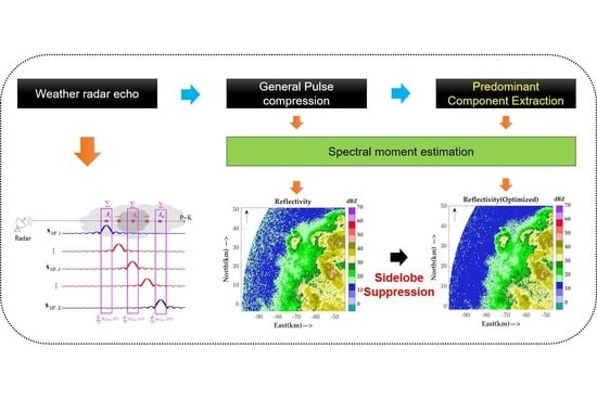
The solid-state transmitters are widely adopted for weather radars, where pulse compression is operated to provide the required sensitivity and range resolution. Therefore, effective sidelobe suppression strategies must be employed, especially for weather observation. Currently, many methods can suppress the sidelobe to a very low level in the case of point targets or uniformly distributed targets. However, in strong convection weather process, the weather echo amplitude lies in a wide dynamic range and the main lobe of weak target is prone to being contaminated by the sidelobe of strong target, causing the degradation of weather fundamental data estimation, even generating artifacts and affecting the quantitative precipitation evaluation. In this paper, we propose a novel strategy which is the further processing of a general pulse compression radar to mitigate the effects of sidelobes. The proposed method is called the predominant component extraction (PCE), in which the re-weighting processing is operated after pulse compression, and then the echo of each bin is optimized and its energy will approach the real targets in each bin. It can improve the estimation of weak signals or even eliminate the artifact at the edge of the scene. Numerical simulation experiments and real-data verifications are implemented to validate the feasibility and superiority. It is noted that the proposed method has no requirement on the transmitted waveform and can be realized only by adding a step after pulse compression in the actual system.

1. Introduction

Pulse compression technology can meet the requirements of high-range resolution and long-range detection at the same time, which has been widely used in weather radar systems with the application of solid-state transmitter.

The commonly used pulse compression waveforms include linear frequency modulation (LFM), nonlinear frequency modulation (NLFM), phase coded signal [1,2,3], etc. The LFM waveform which is the most widely used has high-range sidelobe (−13.26 dB) after matched filtering. A window function is often utilized to suppress range sidelobes, resulting in the expansion of the main lobe and the loss of the signal to noise ratio (SNR) [4,5]. However, the reflectivity of precipitations ranges from about −10 to 75 dBZ [6,7] and the radar sensitivity is one of the most critical factors for distributed precipitations in weather observations. Therefore, in order to reduce the SNR loss of LFM signal after windowing, the NLFM waveform was developed decades ago. The concept of NLFM waveform was put forward by Fowle and Brandon in 1959 [8,9]. The energy spectrum (i.e., the square of the spectrum) of NLFM can be designed as a window function, namely, the effect of windowing can be transferred to signal modulation, and then the matching filter can be performed directly to achieve low sidelobe performance, in order to avoid the SMR loss caused by windowing processing [7]. The peak sidelobe ratio (PSLR) can be reduced to below −40 dB after matched filtering, which can achieve the same results of window function weighting processing [10]. At the same time, NLFM has better detection rate characteristics and more accurate range detection performance than LFM [11].

However, some researches have shown that the adjacent reflectivity in extreme weather targets varies dramatically and the gradient often ranges from 30 to 40 dBZ within 1 km, sometimes even reaching 55 dBZ/km [12,13,14]. In order to realize the detection of weather targets with high gradient-reflectivity phenomenon, a very effective sidelobe suppression strategy must be adopted to avoid the artifact caused by range sidelobes [15], while the sidelobe performances of NLFM waveform are not enough to meet the accuracy of the quantitative detection of distributed scatterers, and the sidelobe needs to be further suppressed.

To reach the ultra-low range sidelobes, a mismatch filter can be used at the cost of losing SNR [5,16,17]. Argenti et al. [12] designed transmit waveforms and receive filters using the quadratic nonlinear optimization method by minimizing both PSLR and integrated sidelobe ratio (ISLR) of the waveform at the receiver output, and the PSLR and ISLR can reach −80 dB and −70 dB, respectively with the loss of resolution degradation. Beauchamp et al. [18] discussed the optimal design of pulse compression waveform/filter pairs for use with near-nadir spaceborne radar in low Earth orbit for the observation of clouds and precipitation. It was demonstrated that the LFM waveforms provide superior performance over NLFM waveforms for the application subject to unmitigated Doppler shifts and the PSLR and ISLR could reach −56 dB and −34 dB, respectively using the minimum integrated sidelobe (ISL) mismatch filter. Kurdzo et al. [15] designed NLFM waveform using a genetic algorithm that took into account individual system characteristics and performance measures in order to design a low SNR loss (high power efficiency) waveform for use with weather radar utilizing pulse compression. In addition, the waveform was implemented in the X-band transportable solid-state dual-polarized weather radar system (PX-1000), and the PSLR and ISLR in the actual system can reach −52 dB and −37 dB, respectively. For weather radar, the received signal of one radar resolution volume (RRV) is the sum of scattered signals from the ensemble of particles in this RRV. Therefore, the velocities of the particles in RVV continuously distribute in an interval and the Doppler spectrum or power spectral density (PSD) generally has Gaussian shape [19]. The spectral moments, i.e., reflectivity, mean radial velocity, and spectrum width (ZVW) are called fundamental weather parameters and are defined as the top three order moments of PSD. Bharadwaj et al. [20] used frequency diversity waveform and minimum ISL mismatch filter for pulse compression. The simulation results show that the estimation errors of fundamental weather parameters, i.e., reflectivity, mean radial velocity, and spectrum width (ZVW) for weak targets will increase when the reflectivity changes greatly, which had been verified using CASA (Center for Collaborative Adaptive Sensing of the Atmosphere) X-band dual-polarized radar.

The sidelobe of the point target from the above-mentioned pulse compression filters can be compressed to a very low level, while it can only be achieved for point or uniformly distributed targets, such as layered precipitation. In the process of strong convection weather phenomenon, the reflectivity will appear as a large gradient, and the sidelobe energy in the strong target range bins will be superimposed into the weak target range bins. When the reflectivity gradient reaches a certain range (such as 40 dBZ/km), the sidelobe energy of the strong target is equal to the main lobe energy of the weak target which will be contaminated, causing the unacceptable estimation errors of ZVW, even generating false targets and affecting the estimation of precipitation [15,21].

Let us assume that the probing of the meteorological object is conducted with frequency modulated waveform (such as LFM or NLFM) at a fixed antenna orientation. After pulse compression of the return signal by the optimal filter (OF), such as matched filter or mismatched filter, some realization of a random echo-signal is received. This signal is a mixture of the amplitudes of the main and sidelobes of the response of the OF, resulting in the increase in estimation error of ZVW. To isolate the reaction of the OF only by the main lobe, in this paper, an artificial realization of the echo-signal is initially modeled. This realization consists only of rectangular pulses with amplitudes obtained by smoothing the amplitudes of the real realization of the echo-signal, which is called basic waveform transfer function (B-WTF) to describe the main lobe signals. Then, considering the parameters of the waveform and OF, the frequency-modulated pulse with amplitudes obtained by smoothing the amplitudes of the real realization of the echo-signal is modeled to describe the sidelobe signals, which is called pulse-compression waveform transfer function (PC-WTF) and is supplemented by the main lobe signals. Thereafter, the cost function of each range bin can be constructed by B-WTF and PC-WTF for the calculations of optimal extraction matrix (OEM) for re-weighting of original real realization. The optimized echoes are used to calculate the relevant data quality index according to some criterions. If the criterions are not satisfied, the iteration procedure is repeated with slightly modified initial conditions until the matching criterion is met. Through the above-mentioned procedure, the predominant signal in each range bin can be extracted from the mixed signal and the sidelobes are cleared.

This method is called the predominant component extraction (PCE), which is operated after pulse compression for a normal weather radar with LFM or NLFM waveform to improve sidelobe suppression. After PCE processing, the energy of optimized echoes will be close to the main lobe energy of the actual targets, achieving the sidelobe suppression of the weather targets with large gradient reflectivity.

When the reflectivity gradient is large, the proposed method can obtain the weak target signal and reduce the estimation errors of ZVW. This optimization effect is particularly clear for the large gradient reflectivity scene in the typhoon or other strong convective weather phenomenon. In addition, this method can significantly improve the data quality and eliminate the artifact at the edge of the scene, which contributes to obtaining the accurate estimation of precipitation and other parameters. It is worth mentioning that the proposed method is operated after pulse compression, and it has no requirement on the radar transmitting waveform, which can be realized by adding a step after pulse compression in the actual radar system.

This article is organized as follows. The optimization model is presented in Section 2. Section 3 describes the calculation of the OEM and the iterative optimization process of the PCE. Some results of simulations and verifications based on the real measured data are shown in Section 4. The discussion is drawn in Section 5. Finally, Section 6 provides the conclusion and research perspectives.

2. Problem Statement and Modeling

Considering one range-direction signal, the normalized echo matrix of unit amplitude transmitted modulation waveform, such as LFM or NLFM after pulse compression is defined as the pulse-compression waveform transfer function (PC-WTF) $s_{MF}$, and the normalized echo matrix with unit amplitude rectangular-pulse transmitted waveform is defined as the basic waveform transfer function (B-WTF) $s_{SP}$, which are expressed as follows:

$$s_{MF}=\left[\begin{array}{c}{s}_{MF,1}\\ s_{MF,2}\\ \begin{array}{c}⋮\\ s_{MF,k}\\ ⋮\end{array}\\ s_{MF,K}\end{array}\right]=\left[\begin{array}{c}{s}_{MF,1}\left(1\right),s_{MF,1}\left(2\right),\cdots ,s_{MF,1}\left(p\right),\cdots ,s_{MF,1}\left(P\right)\\ s_{MF,2}\left(1\right),s_{MF,2}\left(2\right),\cdots ,s_{MF,2}\left(p\right),\cdots ,s_{MF,2}\left(P\right)\\ ⋮\\ s_{MF,k}\left(1\right),s_{MF,k}\left(2\right),\cdots ,s_{MF,k}\left(p\right),\cdots ,s_{MF,k}\left(P\right)\\ ⋮\\ s_{MF,K}\left(1\right),s_{MF,K}\left(2\right),\cdots ,s_{MF,K}\left(p\right),\cdots ,s_{MF,K}\left(P\right)\end{array}\right]$$

(1)

$$s_{SP}=\left[\begin{array}{c}{s}_{SP,1}\\ s_{SP,2}\\ \begin{array}{c}⋮\\ s_{SP,k}\\ ⋮\end{array}\\ s_{SP,K}\end{array}\right]=\left[\begin{array}{c}{s}_{SP,1}\left(1\right),s_{SP,1}\left(2\right),\cdots ,s_{SP,1}\left(p\right),\cdots ,s_{SP,1}\left(P\right)\\ s_{SP,2}\left(1\right),s_{SP,2}\left(2\right),\cdots ,s_{SP,2}\left(p\right),\cdots ,s_{SP,2}\left(P\right)\\ ⋮\\ s_{SP,k}\left(1\right),s_{SP,k}\left(2\right),\cdots ,s_{SP,k}\left(p\right),\cdots ,s_{SP,k}\left(P\right)\\ ⋮\\ s_{SP,K}\left(1\right),s_{SP,K}\left(2\right),\cdots ,s_{SP,K}\left(p\right),\cdots ,s_{SP,K}\left(P\right)\end{array}\right]$$

(2)

where each row of (1) and (2) represents the range direction sample sequence and $P$ is the number of range bins of echoes. Each column represents the normalized amplitude of each target applied to the corresponding range bin, and K is the number of targets. In contrast to point targets, the entire radar beam is usually filled with weather targets; therefore, the number of range bins can be treated as equivalent to the number of targets, i.e., $P=K$. In addition, $s_{MF,k}$ is the PC-WTF of the kth target and $s_{SP,k}$ is the B-WTF of the kth target as follows:

$$s_{MF,k}=\left[s_{MF,k}\left(1\right),s_{MF,k}\left(2\right),\cdots ,s_{MF,k}\left(p\right),\cdots ,s_{MF,k}\left(P\right)\right]$$

(3)

$$s_{SP,k}=\left[s_{SP,k}\left(1\right),s_{SP,k}\left(2\right),\cdots ,s_{SP,k}\left(p\right),\cdots ,s_{SP,k}\left(P\right)\right]$$

(4)

Due to the absence of sidelobes of rectangular-pulse waveform and the presence of sidelobes of pulse compression waveform, $s_{MF,k}\left(p\right)$ and $s_{SP,k}\left(p\right)$ which are the members of (3) and (4), respectively, can be expressed as follows:

$$s_{MF,k}\left(p\right)=\{\begin{array}{cc}{a}_0& p=k\\ b\left(p\right)& p\ne k\end{array}$$

(5)

$$s_{SP,k}\left(p\right)=\{\begin{array}{cc}{a}_0& p=k\\ 0& p\ne k\end{array}$$

(6)

where $a_0$ is the main lobe value after pulse compression of kth target’s echo, $k$ is the range bin position where the main lobe is located, and $b\left(p\right)$ is the sidelobe value at other range bin locations of kth target’s echo.

Therefore, the values of $a_0$ and $b\left(p\right)$ are only related to the waveform parameters, the radar system parameters, and the method of pulse compression, which are independent of the target characteristics. In particular, as long as the waveform parameters, the radar system parameters, and the method of pulse compression are determined, $s_{MF}$ and $s_{SP}$ will be determined. Considering the PC-WTF as an example, its schematic diagram is shown in Figure 1:

Let us assume that $A=\left[\begin{array}{ccc}{A}_1^{}& \begin{array}{ccc}\cdots & A_k^{}& \cdots \end{array}& A_K^{}\end{array}\right]$ is the backscattering coefficient matrix, and $A_k$ is the complex backscattering coefficient of the kth target, where the amplitude is related to the scattering intensity of the target and the phase includes the information of doppler velocity of the target. The received echo is the superposition from all targets as shown in Figure 2, which can be expressed as (7):

$$\begin{array}{cc}{P}_0& =A{s}_{MF}\hfill \\ & =\left[{\displaystyle \sum _{k=1}^K{A}_k{s}_{MF,k}\left(1\right)},{\displaystyle \sum _{k=1}^K{A}_k{s}_{MF,k}\left(2\right)},\cdots ,{\displaystyle \sum _{k=1}^K{A}_k{s}_{MF,k}\left(P\right)}\right]\hfill \end{array}$$

(7)

It can be seen from (7) that the energy of each range bin is the superposition of the main lobe of this bin and the sidelobes from other bins. When the energy of the extra added sidelobes is comparable to that of the original main lobe, it will affect the estimations of ZVW. Therefore, it is considered to re-optimize the signal of each range bin and its energy will approach that of the actual targets in each bin; therefore, we call it the predominant component extraction (PCE) method.

Considering the operation of the weighting processing of the signals in each range bin, we can obtain the weighted signal as follows:

$$P_{est}=A\left(W_{opt}^{}\odot s_{MF}\right)$$

(8)

where $W_{opt}^{}$ is the OEM with $K\times P$ dimension as follows:

$$W_{opt}^{}=\left[\begin{array}{cccccc}{w}_{opt,1}\left(1\right)& w_{opt,2}\left(1\right)& \cdots & w_{opt,p}\left(1\right)& \cdots & w_{opt,P}\left(1\right)\\ w_{opt,1}\left(2\right)& w_{opt,2}\left(2\right)& \cdots & w_{opt,p}\left(2\right)& \cdots & w_{opt,P}\left(2\right)\\ ⋮& ⋮& \cdots & ⋮& \cdots & ⋮\\ w_{opt,1}\left(k\right)& w_{opt,2}\left(k\right)& \cdots & w_{opt,p}\left(k\right)& \cdots & w_{opt,P}\left(k\right)\\ ⋮& ⋮& ⋮& ⋮& ⋮& ⋮\\ w_{opt,1}\left(K\right)& w_{opt,2}\left(K\right)& \cdots & w_{opt,p}\left(K\right)& \cdots & w_{opt,P}\left(K\right)\end{array}\right]$$

(9)

where $w_{opt,p}={\left[\begin{array}{ccc}{w}_{opt,p}\left(1\right)& \cdots & w_{opt,p}\left(K\right)\end{array}\right]}_{}^{\mathrm{T}}$ is the optimization coefficient of pth range bin and $\odot$ is Hadamard product. The signal is weighed using $w_{opt,p}$ in each range bin in order that the energy will approach that of the actual targets. Next, an optimization problem is established by B-WTF to obtain $W_{opt}^{}$.

Since the echoes of rectangular pulse signal only have the main lobe and there is no sidelobe to be superimposed in the other range bins, the calculated signal energies are optimal in theory. Therefore, we can use rectangular waveforms to model the expected output echo:

$$\begin{array}{cc}{P}_{\exp }& =A{s}_{SP}\hfill \\ & =\left[{\displaystyle \sum _{k=1}^K{A}_k{s}_{SP,k}\left(1\right)},{\displaystyle \sum _{k=1}^K{A}_k{s}_{SP,k}\left(2\right)},\cdots ,{\displaystyle \sum _{k=1}^K{A}_k{s}_{SP,k}\left(P\right)}\right]\hfill \\ & =\left[A_1{s}_{SP,1}\left(1\right),A_2{s}_{SP,2}\left(2\right),\cdots ,A_P{s}_{SP,P}\left(P\right)\right]\hfill \end{array}$$

(10)

In order to obtain $P_{\exp }$, $W_{opt}$ needs to meet the following condition:

$$\begin{array}{cc}\underset{W_{opt}}{\min }& p\left(W_{opt}\right)\\ s.t.& p\left(W_{opt}\right)={\Vert P_{est}-P_{\exp }\Vert }_2^2\end{array}$$

(11)

To date, the optimization model has been established.

It should be noted that, in this paper, we assume that the echoes are entirely from meteorological targets and the patterns of targets are determined by the backscattering coefficient matrix and waveform transfer function. However, the PCE method can be operated regardless of how the target is distributed. We do not need to know the value of backscattering coefficient matrix in advance when modeling PC-WTF and B-WTF. As long as the waveform and radar system parameters are determined, PC-WTF and B-WTF can be modeled, which can be realized in the actual processing process. After modeling PC-WTF and B-WTF, what we need to solve is how to optimize (7) to make it closer to (10), which needs to be realized by the PCE method proposed in this paper. The block diagram of the PCE algorithm is presented in Figure 3.

3. Optimization Process

3.1. The Solution of OEM

After obtaining the above-mentioned optimization model, $W_{opt}^{}$ can be calculated by the derivative of $p\left(W_{opt}\right)$ and setting the derivative to zero. Next, we will introduce the calculation process in detail.

Expanding (11), we can achieve:

$$\begin{array}{cc}\underset{W_{opt}}{\min }& p\left(W_{opt}\right)\\ s.t.& p\left(W_{opt}\right)={\Vert A\left(W_{opt}^{}\odot s_{MF}\right)-A{s}_{SP}\Vert }_2^2\end{array}$$

(12)

For distributed meteorological targets, P = K can be assumed and A is a matrix that does not change in one coherent processing interval (CPI). At this time, a unit matrix $I$ can be introduced to facilitate the derivative calculation of Hadamard product. Then, the above-mentioned optimization problem can be written as:

$$\begin{array}{cc}\underset{W_{opt}}{\min }& p\left(W_{opt}\right)\\ s.t.& p\left(W_{opt}\right)={\Vert \left(W_{opt}^{}I\odot s_{MF}\right)-s_{SP}\Vert }_2^2\end{array}$$

(13)

Additionally, $W_{opt}^{}$ can be calculated from $\frac{d\left[p\left(W_{opt}\right)\right]}{d{W}_{opt}}=0$, as shown in (14), where the detailed calculation process is in Appendix A.

$$W_{opt}^{}={\left(I\odot s_{MF}\odot s_{MF}{I}^{\mathrm{T}}\right)}^{-1}\left(I\odot s_{MF}{s}_{SP}\right)$$

(14)

3.2. Iteration Process

After obtaining $W_{opt}^{}$, the echoes can be optimized through formula (8). However, the initial matrix $A$ needs to be known. Thereafter, the data quality can be improved through iteration. If the actual received echo is $S_r$, we can express it as:

$$S_r=A{s}_{MF}$$

(15)

A can be calculated as:

$$A={\left[{\left(s_{MF}^{\mathrm{T}}\right)}^{-1}{S}_r^{\mathrm{T}}\right]}_{}^{\mathrm{T}}$$

(16)

Then, the estimated echo by the PCE method can be expressed as:

$$S_{est}=A\left(W_{opt}^{}\odot s_{MF}\right)$$

(17)

Thereafter, the OEM of (17) is recalculated and optimized iteratively until the stop criterion is met. Next, we set the appropriate stop criterion to make the data quality meet the requirements.

Since the proposed method in this paper is not aimed at the point target sidelobe, the performance of PSLR and ISLR cannot be compared. Therefore, other indicators that can reflect the data quality need to be set as the stop criterion.

• Data error iteration condition:

The root mean square error (RMSE) reflects the degree of data deviation from the ground truth. In the quantitative analysis of simulation, the ground truth is given; therefore, the stop criterions can be set according to the RMSE. The RMSE of one range direction can be calculated as:

$$RMS{E}_E=\sqrt{\frac{1}{P}{\displaystyle \sum _{p=1}^P{\left|E_{est}\left(p\right)-E_{gt}\left(p\right)\right|}^2}}$$

(18)

where $E_{est}$ represents the ZVW (i.e., reflectivity $Z_{est}$, radial velocity $V_{est}$, and spectral width $W_{est}$) calculated from the optimized echoes and $E_{gt}$ is the ground truth of ZVW.

Since the energy optimization effect of each range bin is our concern in this paper, we can set the RMSE of the reflectivity less than a certain threshold ${\epsilon }_1$ as the stop criterion, as follows:

$$RMS{E}_{Z_{est}}<{\epsilon }_1$$

(19)

• Data fluctuation iteration condition:

In real-data verification, the ground truth cannot be obtained, while the moving average can be used as the ground truth to calculate SD. Therefore, the SD can reflect the fluctuation of radar data and we call it data fluctuation, which can be used to set the stop criterion. The standard deviation (SD) of ZVW in the pth range bin can be calculated by the data on n range bins before and n range bins after, and the first n range bins and the last n range bins do not participate in the calculation of SD [22]:

$$\begin{array}{l}S{D}_p=\sqrt{\frac{1}{2n+1}{\displaystyle \sum _{j=0}^{2n+1}{\left(E_{p+j-n}-{\overline{E}}_p\right)}^2}},0<n<\frac{P}{2},n<p<P-n\\ {\overline{E}}_p=\frac{1}{2n+1}{\displaystyle \sum _{j=0}^{2n+1}{E}_{p+j-n},}0<n<\frac{P}{2},n<p<P-n\end{array}$$

(20)

where $E$ represents the ZVW (i.e., reflectivity $Z_{est}$, radial velocity $V_{est}$, and spectral width $W_{est}$) calculated from the optimized echoes. ${\overline{E}}_p$ is the moving average calculated from $2n+1$ range bins.

Setting the percentage of data with the SD less than 1 in the total data greater than ${\epsilon }_2$ as the stop criterion, we can make the data fluctuation meet the requirements. This percentage is defined as the data fluctuation qualification rate AR, as follows:

$$AR=\frac{\mathrm{sum}\left(S{D}_p<1\right)}{P}\times 100\%>{\epsilon }_2,0<{\epsilon }_2<100\%$$

(21)

In summary, Algorithm 1 can be summarized as follows.

Algorithm 1: The PCE algorithm

◆ STEP 1: Model the PC-WTF and B-WTF according to the radar system and waveform parameters. ◆ STEP 2: Calculate $W_{opt}^{}$ according to (14). ◆ STEP 3: Calculate the initial matrix $A$ according to (16). ◆ STEP 4: Calculate the first optimization echo $S_{est}^{}$ according to (17) and estimate the spectral moments, i.e., $Z_{est}^{}$, $V_{est}^{}$, and $W_{est}^{}$. ◆ STEP 5: In the quantitative analysis of simulation stage, calculate the RMSE and AR of $Z_{est}^{}$ and set the iteration thresholds ${\epsilon }_1$ and ${\epsilon }_2$ Judge whether the stop criterion of (19) and (21) are met. In the real-data verification stage, calculate the AR of $Z_{est}^{}$ and set the iteration threshold ${\epsilon }_2$ Judge whether the stop criterion of (21) is met. ◆ STEP 6: Repeat steps 3 to 5 until the stop criterion is satisfied.

4. Results

Before the distributed target simulation, first, the point target scene is simulated and the performances of PSLR and ISLR of four different pulse compression methods are compared, i.e., LFM waveform with windowing, LFM waveform with mismatch filtering, NLFM waveform with windowing, and NLFM waveform with mismatch filtering, wherein the NLFM signal is constructed according to [23] and the mismatch filter is constructed according to the method in [24]. Then, the input ZVW is used to simulate one-dimensional echoes of distributed targets in the range direction. The pulse compression method with the best performance is used for processing. The pulse pair processing method (PPP) is used for spectral moment estimation [21]. This processing set can explain the influence of sidelobe superposition of distributed meteorological targets. Thereafter, the PCE method is used and the RMSE and AR are calculated through (18) and (21) to quantitatively analyze the advantages of the proposed method. Finally, the real in-phase and quadrature-phase (I/Q) data of an actual supercell from a ground-based weather radar and global precipitation measurement (GPM) precipitation data are obtained, which are applied to the proposed method for verification.

4.1. Verifications Based on Numerical Simulation Experiments

4.1.1. Sidelobe Superposition Effects

First, the echo of point target is simulated, and the parameters are shown in

Table 1. The simulation parameters of point target.

Parameters	Values
Frequency (GHz)	13.6
Band width (MHz)	4
Pulse width (μs)	64
Sample frequency (MHz)	16
Target distance (km)	15

. The processing results using different pulse compression methods are in Figure 4, where the window function is Hamming window function.

The performances of the four pulse compression methods are shown in

Table 2. The performances of the four pulse compression methods.

	LFM (MF + W)	LFM (WMMF)	NLFM (MF + W)	NLFM (WMMF)
PSLR (dB)	−53.34	−55.31	−60.97	−67.89
ISLR (dB)	−25.66	−27.84	−28.94	−37.23
SNR loss (dB)	6.12	1.84	3.16	0.14

, where “W” refers to the windowing process. It can be indicated that the windowing process will cause serious SNR loss and the loss of SNR can be mitigated by using NLFM waveform. In addition, the performances of the combination of NLFM waveform and mismatch filter are best, which can suppress PSLR and ISLR below −60 dB and −35 dB, respectively.

Next, the one-dimensional echoes of distributed targets with different reflectivity gradients are simulated. The simulation parameters are shown in

Table 3. The simulation parameters of one-dimensional echoes of distributed targets with different reflectivity gradients.

Parameters	Values	Parameters	Values
Frequency (GHz)	13.6	Pulse width (μs)	64
Band width (MHz)	4	Sample frequency (MHz)	16
Accumulation pulse number	64	PRF (Hz)	1860/1395
Target number	350	Gradient of Z (dBZ/km)	15/25/40
Target spectral width (m/s)	Randi [1, 5]	Target velocity (m/s)	Int [−7, 7]

, where the SNR of the input signal is 60 dB. The target number is equal to 350, which is equivalent to the total range bin number. The range revolution is 37.5 m and the detection distance is 13.125 km. In addition, the weak targets account for 7.5 km and the strong targets account for 3.6 km. The transmit waveform is NLFM in [23] and the mismatch filter in [24] is used for pulse compression. The input Z with different gradients is shown in Figure 5. In addition, the reflectivity, mean velocity, and spectral width can be obtained by the PPP method in Figure 6, Figure 7 and Figure 8, respectively.

Although the performance of the pulse compression method is good enough, when the reflectivity gradient is large (such as 40 dBZ/km), the energy of the sidelobe of the strong target is equal to or even greater than the energy of the weak target, resulting in the estimation errors of the ZVW in the weak target area.

4.1.2. Optimization Process

In order to solve the above-mentioned problems, the PCE algorithm is used for each range bin. The comparison results are shown in Figure 9, Figure 10 and Figure 11. The RMSE and AR of ZVW before and after optimization can be calculated through (18) and (21), respectively. The results are shown in

Table 4. The RMSE and AR of ZVW (not optimized/optimized).

$\mathbf{Gradient} \mathbf{of} \mathbf{Z}$ (ΔZ, dBZ/km)		15	25	40
Z (dBZ)	RMSE (dBZ)	2.65/2.32	3.30/2.34	10.42/4.23
	AR (%)	24.57/50.01	32.37/45.66	28.90/28.61
V (m/s)	RMSE (m/s)	2.02/1.14	2.93/1.20	4.13/1.61
	AR (%)	39.02/85.84	28.61/82.95	36.99/49.42
W (m/s)	RMSE (m/s)	1.92/0.72	1.99/0.69	2.01/1.56
	AR (%)	36.13/50.87	45.66/48.84	39.60/59.54

.

It can be indicated that the RMSE and AR can be improved by the proposed method. Moreover, we calculate the RMSE and AR changing with the gradient of reflectivity in the range of 10~40 dBZ/km. The results are shown in Figure 12 and Figure 13. When the reflectivity gradient is large (≥30 dBZ/km), the Z and V estimations are seriously deviated from the ground truth due to the fact that the RMSEs are large. At this time, the data are invalid and the calculated AR is not referential. The proposed method can greatly reduce the RMSE, in order that the invalid data can become valid. When the reflectivity gradient is not large (<30 dBZ/km), the RMSE is acceptable and the data are valid. At this time, we focus on the results of AR. The ARs of optimized data are more acceptable and the data quality is effectively improved.

In addition, we compared the SNR loss caused by the proposed method. In contrast to point targets, the distributed targets cannot directly compare the energy of the main lobe. Therefore, the SNR loss is defined as the mean difference SNR before and after optimization:

$$SNRloss=\frac{1}{P}{\displaystyle \sum _{p=1}^P\left[SN{R}_{before}\left(p\right)-SN{R}_{after}\left(p\right)\right]}$$

(22)

The SNR loss changing with reflectivity gradient is shown in Figure 14. It can be indicated that with the increase in reflectivity gradient, SNR loss will become serious. Therefore, the proposed method is to improve the data quality at the cost of loss of SNR.

4.2. Verifications Based on Real Data

4.2.1. Verifications by Ground-Based Weather Radar Data

The radar is located at WRCP station (32.75°N, 119.35°E) with an altitude of 32.3 m and works in the conical scanning mode with the azimuth angle of 0 to 360 degrees. The operating parameters are listed in

Table 5. The operating parameters of ground-based weather radar.

Parameters	Value	Parameters	Value
Frequency (GHz)	5.5	Peak Power (W)	1710
Antenna gain (dB, T/R)	34/38	Beam width (°, AZ/EL)	1/3
Noise figure (dB)	3	Pulse number	32
Pulse width (μs)	100	Bandwidth (MHz)	1
Dual PRF (Hz)	900/1200	Elevation angle (°)	2

.

Supercells, as one of the important mesoscale weather systems, can form severe convective weather, such as heavy precipitation, thunderstorm wind, hail, and tornado. In the radar map, the supercell appears as a tightly organized image of high reflectivity, which may have a hook echo. The in-phase and quadrature(I/Q) data originated from a supercell appearing in 22:52 UTC on 17 July 2020. The echo data contained 902 CPI, 32 pulses per CPI, and 652 range gates per pulse. The transmit waveform is LFM and the matched filtering and Hamming window are used.

The ZVWs of the supercell are shown in Figure 15 and the results after optimization by PCE are shown in Figure 16. Due to the large scale of the supercell, the contrast result is not clear in the complete image. Since the proposed method improved the reflectivity (i.e., echo power) significantly, we enlarged the local reflectivity for comparison as shown in Figure 17. We can see that the artifacts at the scene edge are basically removed after optimization and the target edge is clearer due to the fact that the sidelobe is suppressed.

The ARs of the ZVW are calculated in

Table 6. The AR of the ZVW.

	Z	V	W
The AR before optimization (%)	62.68	64.90	76.39
The AR after optimization (%)	70.66	70.20	84.54

. It can be indicated that the percentages of ZVW with the SD less than 1 in total data are increased after optimization, which indicated the effective improvement of the data quality.

4.2.2. Verifications by Quantitative Precipitation Estimation (QPE) Data

In order to verify the application value of the proposed method, we use the Z–I relationship to estimate the precipitation in positions A and B, in which Z is the reflectivity calculated by the unoptimized data and optimized data, respectively, and I is the precipitation intensity in mm/h. The same Z–I relationship is used for both, which is $Z=70I^{1.38}$ fitted from a supercell in [25].

The ground truth of precipitation is the global precipitation measurement (GPM) from Goddard Earth Sciences Data and Information Services Center (GES) DISK) [26] with a time resolution of 0.5 h and a spatial resolution of 0.1°× 0.1°.

In positions A and B, we select 3 × 3 pixels with an adjacent distance of 10 km. For each pixel, the reflectivity of the range bins within the four surrounding spatial resolutions (0.1° × 0.1°) is extracted to calculate the precipitations which are averaged successively, and the precipitation estimates at the pixel can be obtained. The selected region is shown in Figure 18. The precipitations at nine pixel points in the two scenes are calculated using the optimized and unoptimized reflectivity and the results are compared as shown in Figure 19. Then, the differences between the estimation and ground truth for optimized and unoptimized data are calculated to obtain the estimation errors as shown in Figure 20.

It is indicated that the precipitations calculated by the optimized reflectivity are more accurate and the RMSE is effectively decreased for the convective region (Position A) that has large gradient reflectivity, which indicates that the proposed method can improve the quality of precipitation estimation. For the stratified precipitation with low rainfall (Position B), the improvement effect is not clear. Therefore, the proposed method is more suitable for strong convection weather targets.

To date, the application value of the proposed method in this paper is illustrated by the real data of ground-based weather radar and QPE data. This method can eliminate artifacts at the edge of the scene and improve the data quality of ZVW and precipitation.

5. Discussion

In the numerical simulation experiments, the performances of the combination of NLFM waveform and mismatch filter are best, which can suppress PSLR and ISLR below −60 dB and −35 dB, respectively. Then, this pulse compression method is used in the distributed targets with different reflectivity gradients, while the energy of the sidelobe of the strong target is equal to or even greater than the energy of the weak target when the reflectivity gradient is large, resulting in the estimation errors of the ZVW in the weak target area, as shown in Figure 6, Figure 7 and Figure 8. It is indicated that the point target performance (such as PSLR and ISLR) of the pulse compression method is good enough, while it cannot meet the requirement of the high-gradient reflectivity distributed targets. At this time, if we operate the PCE algorithm after pulse compression, the weak targets can be reconstructed and the ZVW can be calculated more accurately, as shown in Figure 12 and Figure 13. In addition, the RMSE and AR results in Figure 12 and Figure 13 can verify the better performance of the PCE algorithm.

Furthermore, in real-data verification, the ground-based weather radar data and QPE data are used to validate the feasibility and superiority of the proposed method. First, the PCE algorithm can eliminate the artifact in the scene and the contour edge of reflectivity is smoother, as shown in Figure 16. In addition, the percentages of ZVW with the SD less than 1 in total data are increased after optimization, as shown in Table 6. These results indicated the effective improvement of the data quality after PCE algorithm. Finally, the precipitations calculated by the optimized reflectivity are more accurate, especially for the convective region as shown in Figure 19 and Figure 20, indicating the advancement of the proposed method in the precipitation estimation.

6. Conclusions

In this paper, a novel sidelobe suppression strategy based on the extraction and iteration of weather radar called PCE is proposed. The cost function is constructed by modeling the transfer function of each range bin for the calculations of OPE. Through PCE processing, the energy of optimized echoes will be close to the main lobe energy of the actual targets in this range bin, achieving the sidelobe suppression of the weather targets with large gradient reflectivity. The proposed method is operated after pulse compression and it has no requirement on the radar transmitting waveform, which can be realized by adding a step after pulse compression in the actual radar system.

It is indicated from numerical simulation experiments that when the reflectivity gradient is large, the proposed method can greatly reduce the estimation errors for weak target, which is at the cost of loss of SNR. When the reflectivity gradient is not large, the data qualities are also effectively improved. The real-data verifications indicate that the proposed method can eliminate artifacts at the edge of the scene and improve the data quality of ZVW and precipitation.

Furthermore, although we only used the measured radar data of supercells to verify the proposed method in this paper, the method can also be applied to other strong convective weather phenomenon such as eyewall of a hurricane and a convective cell. These will be studied in the follow-up work.

References

Skolnik, M.I. Radar Handbook, 3rd ed.; McGraw-Hill: New York, NY, USA, 2008. [Google Scholar]
Richards, M.A. Fundamentals of Radar Signal Processing; McGraw-Hill Processional: New York, NY, USA, 2005. [Google Scholar]
Cook, E.; Bernfeld, M. Radar Signals—An Introduction to Theory and Applications; Artech House: Norwood, MA, USA, 1993. [Google Scholar]
Griffiths, H.D.; Vinagre, L. Design of Low-Sidelobe Pulse Compression Waveforms. Electron. Lett.1994, 30, 1004–1005. [Google Scholar] [CrossRef]
Bringi, V.N.; Chandrasekar, V. Polarimetric Doppler Weather Radar: Principles and Applications; Cambridge University Press: Cambridge, UK, 2001. [Google Scholar]
Pang, C.; Hoogeboom, P.; Le Chevalier, F.; Russchenberg, H.W.; Dong, J.; Wang, T.; Wang, X. A Pulse Compression Waveform for Weather Radars with Solid-State Transmitters. IEEE Geosci. Remote Sens. Lett.2015, 12, 2026–2030. [Google Scholar] [CrossRef]
Brandon, P.S. The Design of a Nonlinear Pulse Compression System to Give a Low Loss High Resolution Radar Performance. Marconi Rev.1973, 36, 1–45. [Google Scholar]
Fowle, E. The Design of FM Pulse Compression Signals. IEEE Trans. Inform. Theory1964, 10, 61–67. [Google Scholar] [CrossRef]
Patton, L.K. On the Satisfaction of Modulus and Ambiguity Function Constraints in Radar Waveform Optimization for Detection. Ph.D. Thesis, Wright State University, Dayton, OH, USA, 2009. [Google Scholar]
Luszczyk, M.; Labudzinski, A. Side Lobe Level Reduction for Complex Radar Signals with Small Base. In Proceedings of the 2012 13th International Radar Symposium, Warsaw, Poland, 23–25 May 2012; pp. 146–149. [Google Scholar]
Argenti, F.; Facheris, L. Radar Pulse Compression Methods Based on Nonlinear and Quadratic Optimization. IEEE Trans. Geosci. Remote Sens.2021, 59, 3904–3916. [Google Scholar] [CrossRef]
Hu, J.; Dong, X.; Hu, C. Research on Nonlinear Wind Field Retrieval Method Based on Modified VAD Analysis. J. Signal Process.2021, 37, 284–291. [Google Scholar] [CrossRef]
Wang, X.; Zhai, W.; Greco, M.; Gini, F. Cognitive Sparse Beamformer Design in Dynamic Environment via Regularized Switching Network. IEEE Trans. Aerosp. Electron. Syst.2022, 59, 1816–1833. [Google Scholar] [CrossRef]
Kurdzo, J.M.; Cheong, B.L.; Palmer, R.D.; Zhang, G.; Meier, J.B. A Pulse Compression Waveform for Improved-Sensitivity Weather Radar Observations. J. Atmos. Ocean. Technol.2014, 31, 2713–2731. [Google Scholar] [CrossRef]
Ackroyd, M.H.; Ghani, F. Optimum Mismatched Filters for Sidelobe Suppression. IEEE Trans. Aerosp. Electron. Syst.1973, AES-9, 214–218. [Google Scholar] [CrossRef]
Cohen, M.N.; Baden, J.M. Pulse Compression Coding Study; Georgia Tech Research Institute: Atlanta, GA, USA, 1983. [Google Scholar]
Beauchamp, R.M.; Tanelli, S.; Peral, E.; Chandrasekar, V. Pulse Compression Waveform and Filter Optimization for Spaceborne Cloud and Precipitation Radar. IEEE Trans. Geosci. Remote Sens.2017, 55, 915–931. [Google Scholar] [CrossRef]
Cavallaro, S. Statistical Properties of Polarimetric Weather Radar Returns for Nonuniformly Filled Beams. IEEE Geosci. Remote Sens. Lett.2017, 14, 1584–1588. [Google Scholar] [CrossRef]
Bharadwaj, N.; Chandrasekar, V. Wideband Waveform Design Principles for Solid-State Weather Radars. J. Atmos. Ocean. Technol.2012, 29, 14–31. [Google Scholar] [CrossRef]
Dong, X.; Hu, J.; Hu, C.; Chen, Z.; Li, Y. Rapid Identification and Spectral Moment Estimation of Non-Gaussian Weather Radar Signal. IEEE Trans. Geosci. Remote Sens.2022, 60, 1–12. [Google Scholar] [CrossRef]
Li, S.; Yang, M.; Li, L. Evaluation on Data Quality of X-Band Dual Polarization Weather Radar Based on Standard Deviation Analysis. J. Arid Meteorol.2019, 37, 467–476. [Google Scholar]
Levanon, N.; Mozeson, E. Radar Signals; Wiley: Hoboken, NJ, USA, 2004. [Google Scholar]
Sun, Y.; Liu, Q.; Cai, J.; Long, T. A Novel Weighted Mismatched Filter for Reducing Range Sidelobes. IEEE Trans. Aerosp. Electron. Syst.2019, 55, 1450–1460. [Google Scholar] [CrossRef]
He, K.; Fan, Q.; Li, K. Z-R Relation with Its Application to Typhoon Precipitation in Zhoushan. J. Appl. Meteorol.2007, 18, 573–576. [Google Scholar]
Huffman, G.J.; Stocker, E.F.; Bolvin, D.T.; Nelkin, E.J.; Tan, J. GPM IMERG Final Precipitation L3 Half Hourly 0.1 Degree x 0.1 Degree V06 2019; Goddard Earth Sciences Data and Information Services Center (GES DISC): Greenbelt, MD, USA, 2019. [Google Scholar]
Zhang, X. Matrix Analysis and Applications; Tsinghua University Press: Beijing, China, 2013. [Google Scholar]
Figure 1.
The schematic diagram of PC-WTF.
Figure 2.
The schematic diagram of received echoes.
Figure 3.
The block diagram of the PCE algorithm.
Figure 4.
The pulse compression results of point target.
Figure 5.
The input Z with different gradients. (a) Gradient of Z is 15 dBZ/km; (b) gradient of Z is 25 dBZ/km; (c) gradient of Z is 40 dBZ/km.
Figure 6.
The reflectivity calculated from unoptimized echoes. (a) Gradient of Z is 15 dBZ/km; (b) gradient of Z is 25 dBZ/km; (c) gradient of Z is 40 dBZ/km.
Figure 7.
The mean velocity calculated from unoptimized echoes. (a) Gradient of Z is 15 dBZ/km; (b) gradient of Z is 25 dBZ/km; (c) gradient of Z is 40 dBZ/km.
Figure 8.
The spectral width calculated from unoptimized echoes. (a) Gradient of Z is 15 dBZ/km; (b) gradient of Z is 25 dBZ/km; (c) gradient of Z is 40 dBZ/km.
Figure 9.
The comparison results of reflectivity. (a) Gradient of Z is 15 dBZ/km; (b) gradient of Z is 25 dBZ/km; (c) gradient of Z is 40 dBZ/km.
Figure 10.
The comparison results of mean velocity. (a) Gradient of Z is 15 dBZ/km; (b) gradient of Z is 25 dBZ/km; (c) gradient of Z is 40 dBZ/km.
Figure 11.
The comparison results of spectral width. (a) Gradient of Z is 15 dBZ/km; (b) gradient of Z is 25 dBZ/km; (c) gradient of Z is 40 dBZ/km.
Figure 12.
The RMSE of ZVW changing with the gradient of reflectivity. (a) Reflectivity; (b) mean velocity; (c) spectral width.
Figure 13.
The AR of ZVW changing with the gradient of reflectivity. (a) Reflectivity; (b) mean velocity; (c) spectral width.