


Real-Time Water Level Monitoring Based on GNSS Dual-Antenna Attitude Measurement


Abstract
1. Introduction
2. Methodology
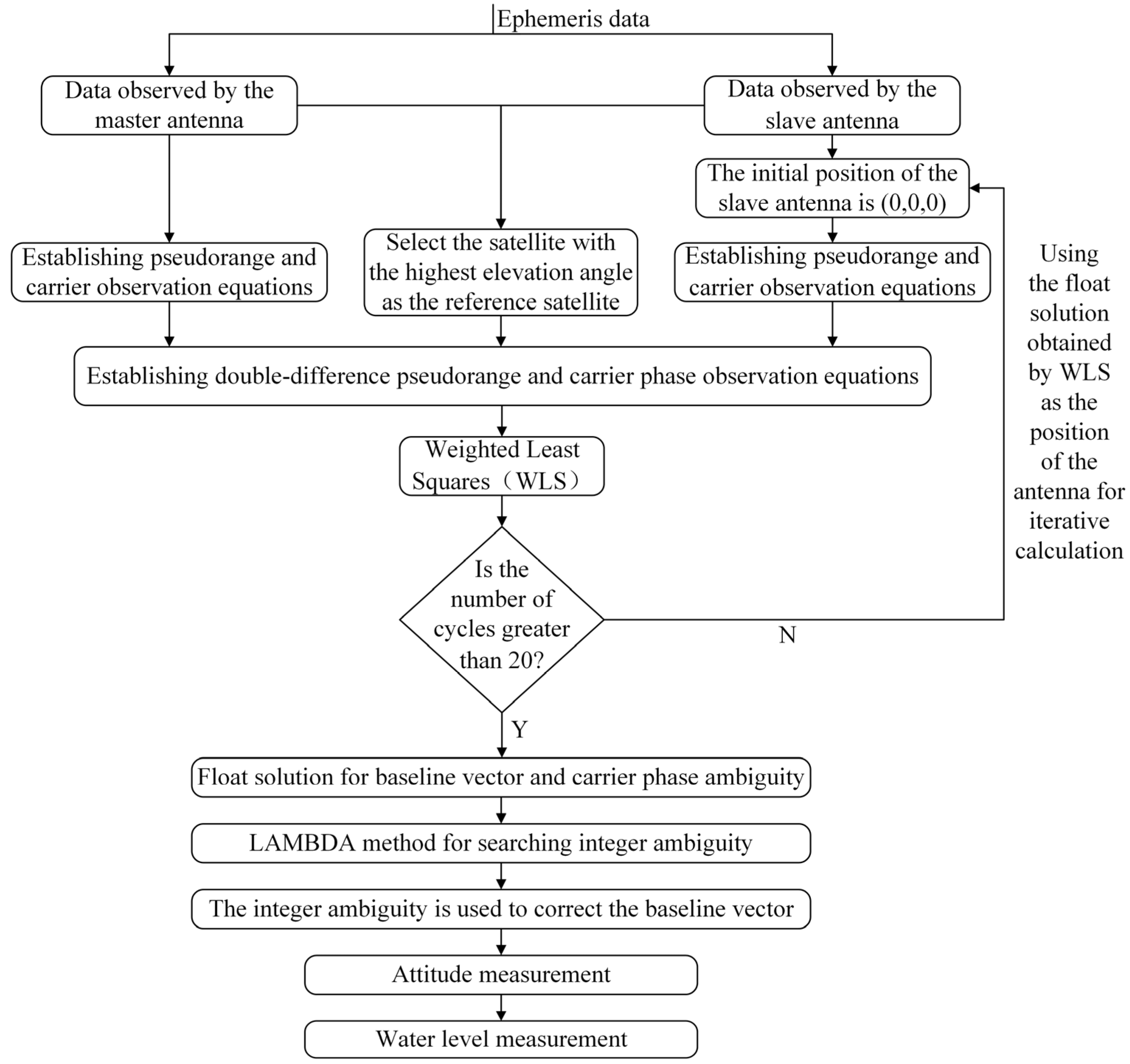
2.1. Program Design
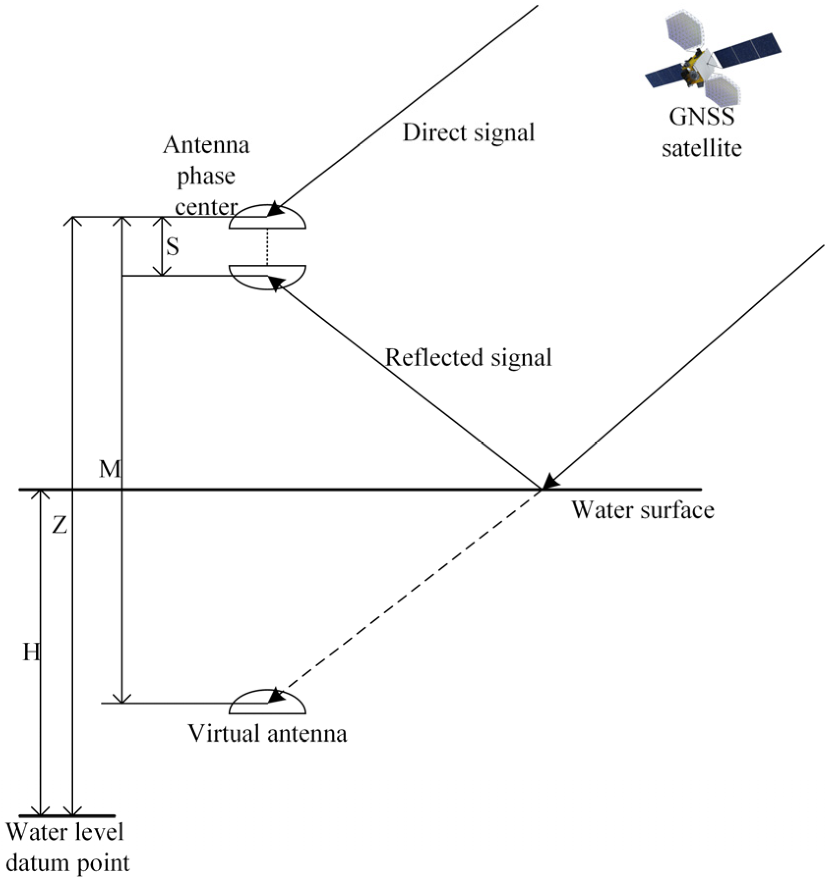
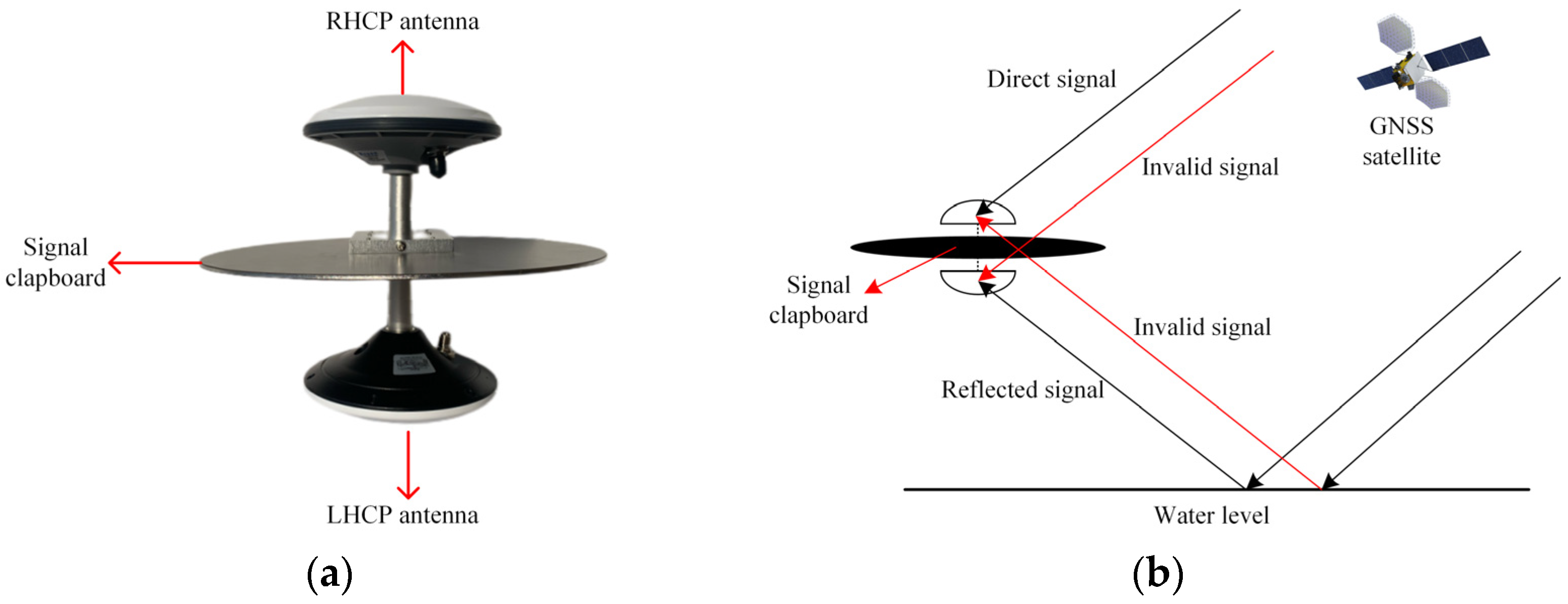
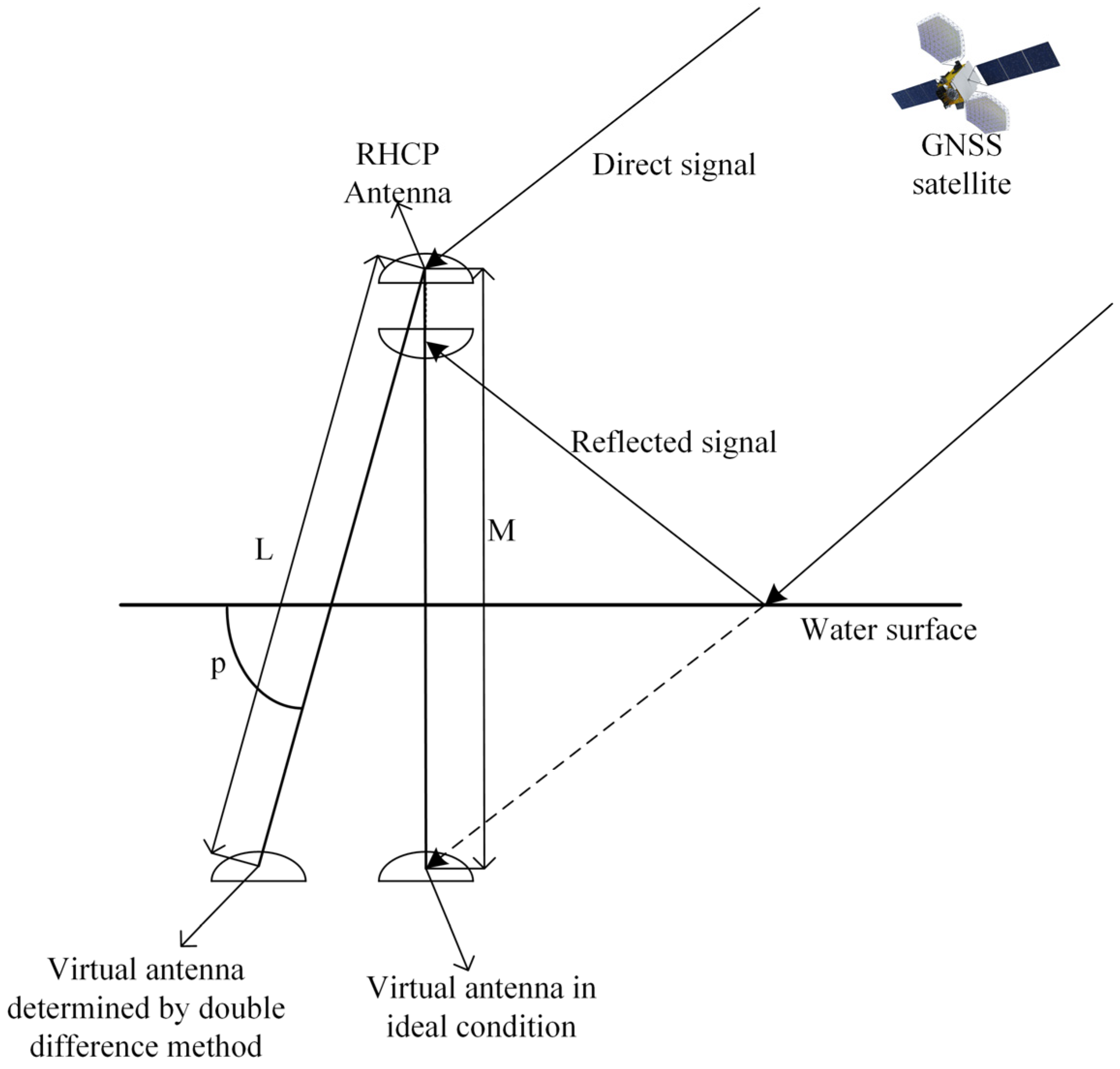
2.2. Altimetry Principle
2.3. Baseline Vector Calculation
2.4. Fixing of Integer Ambiguity
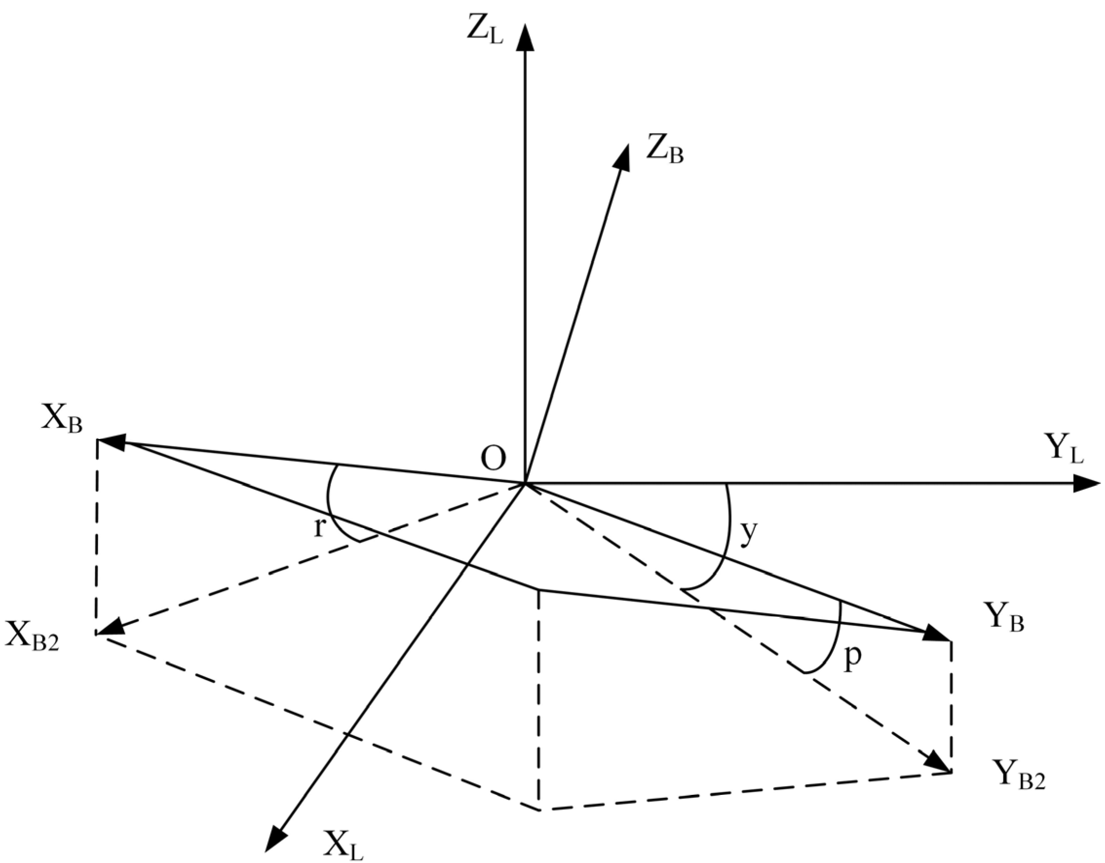
2.5. Definition and Calculation of Attitude Angle
2.5.1. Definition of Attitude Angle
2.5.2. Calculation of Attitude Angle
3. Field Experiment
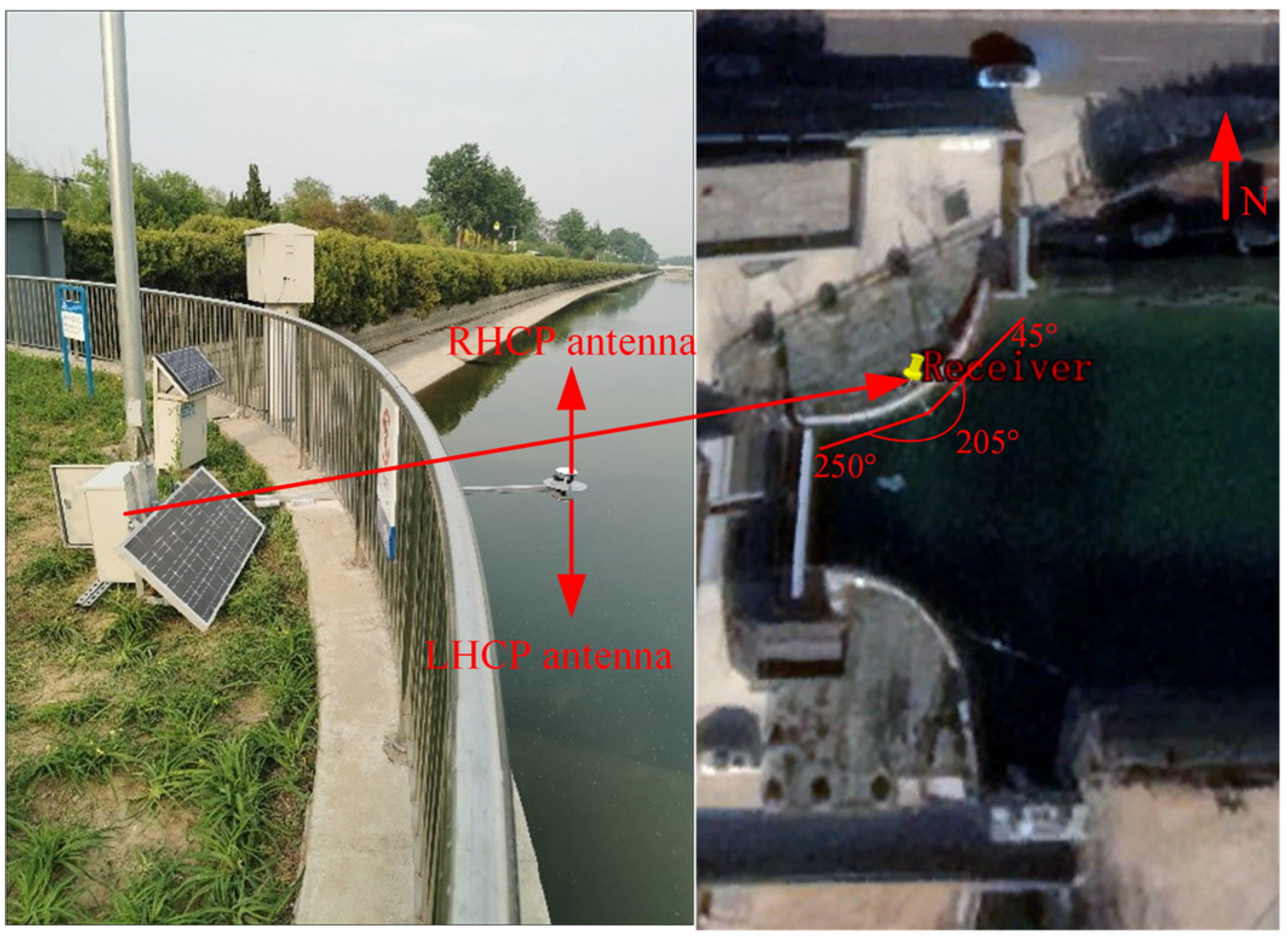
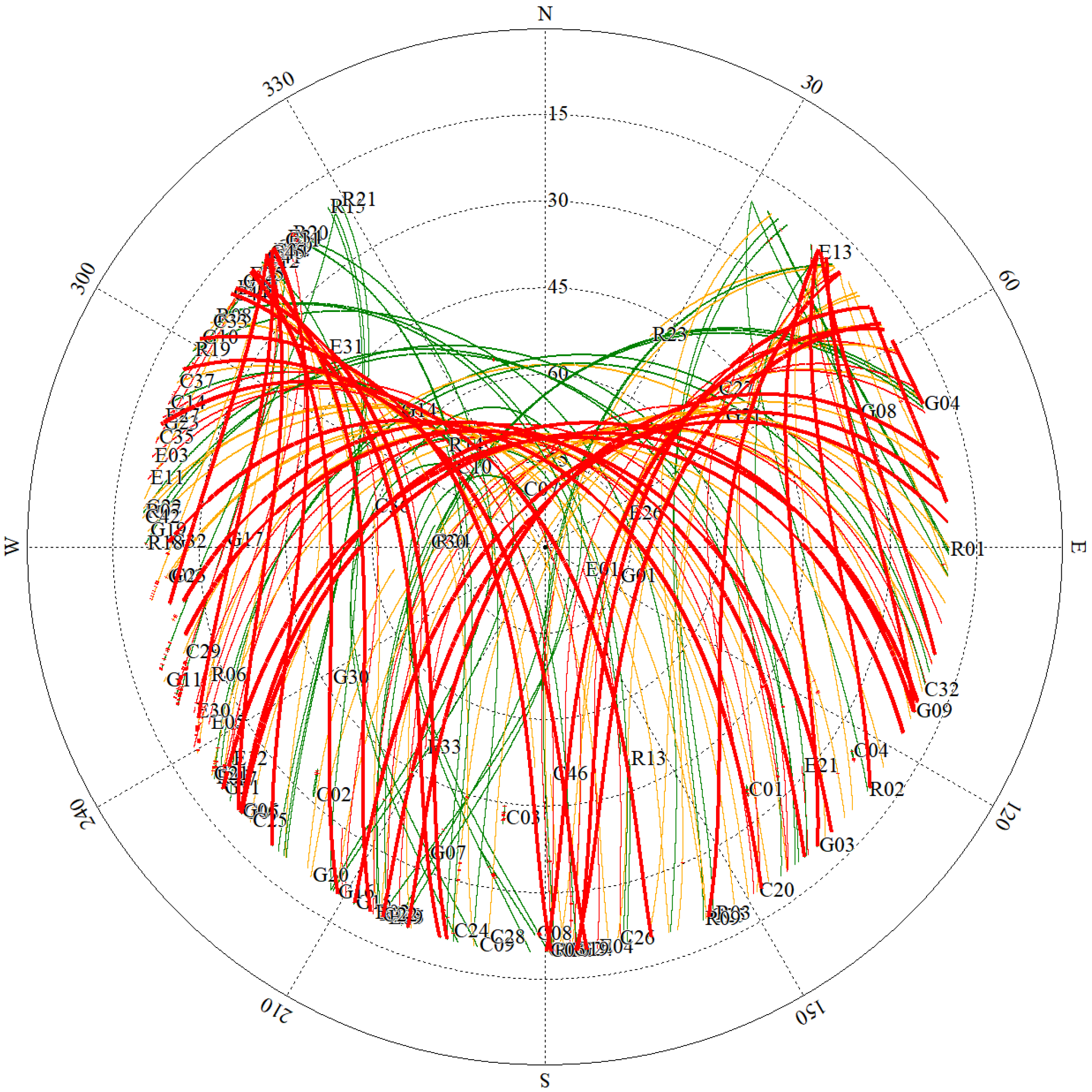
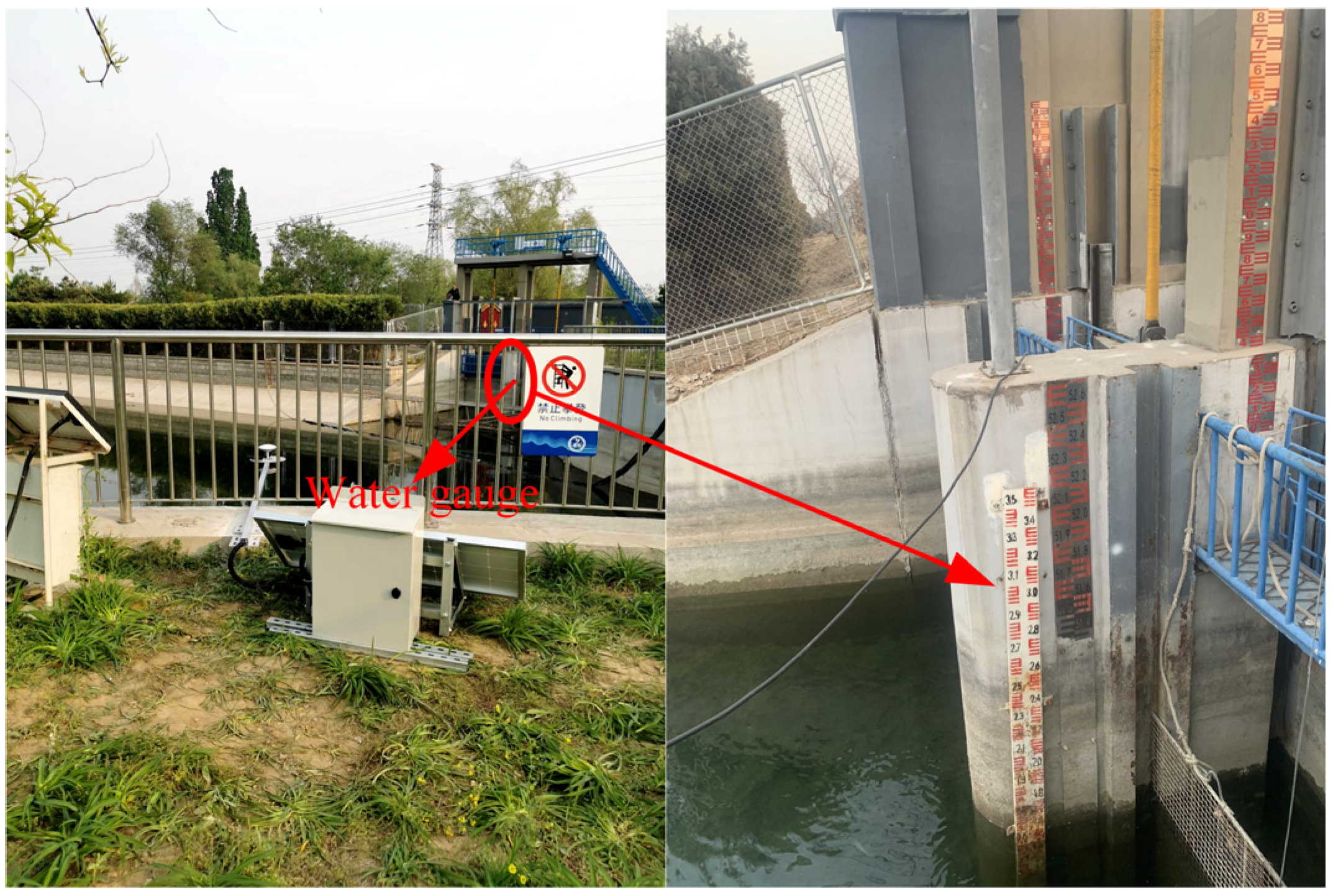
3.1. Experimental Scenario
3.2. Experimental Equipment
4. Results
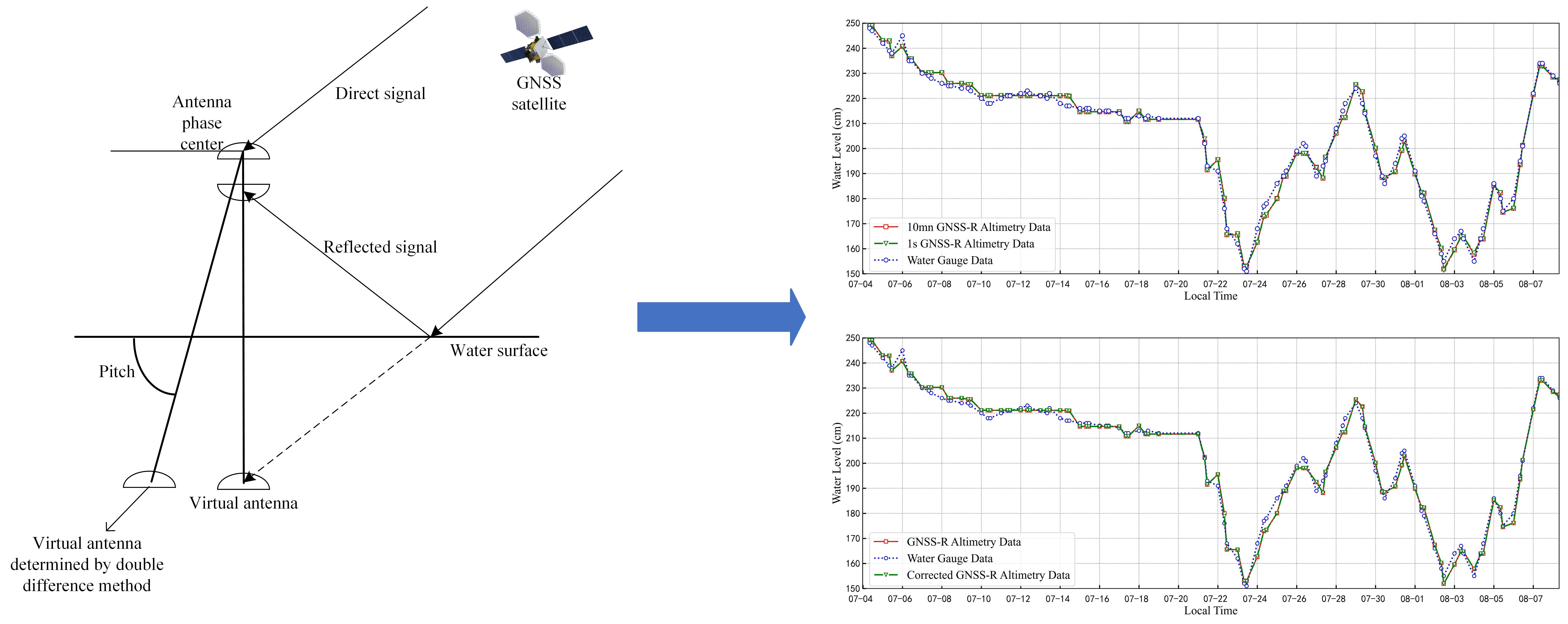
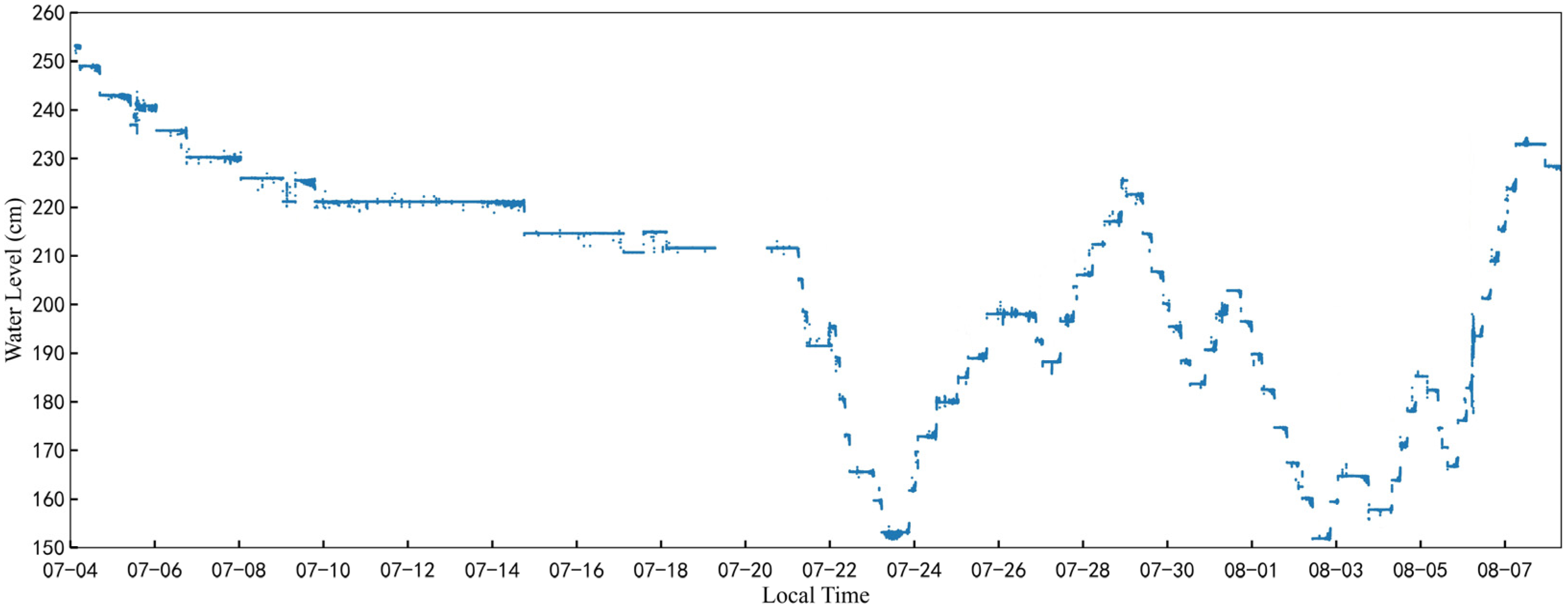
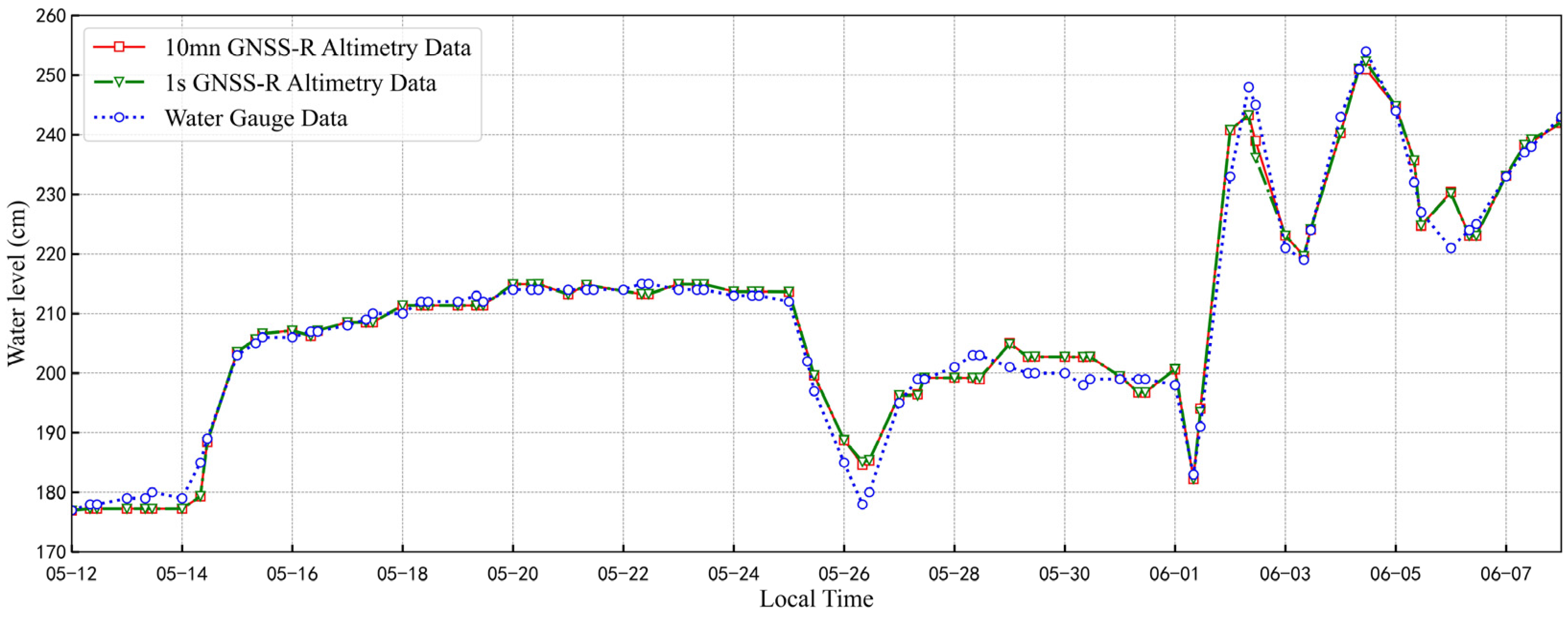
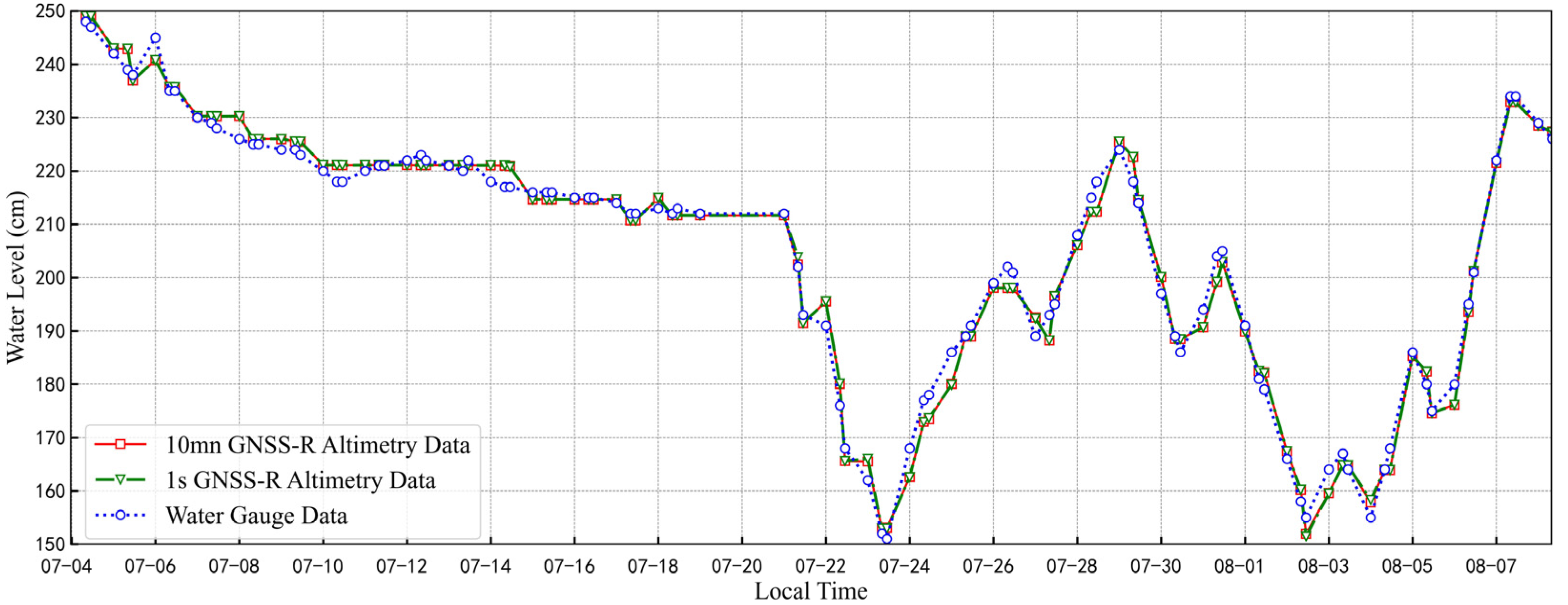
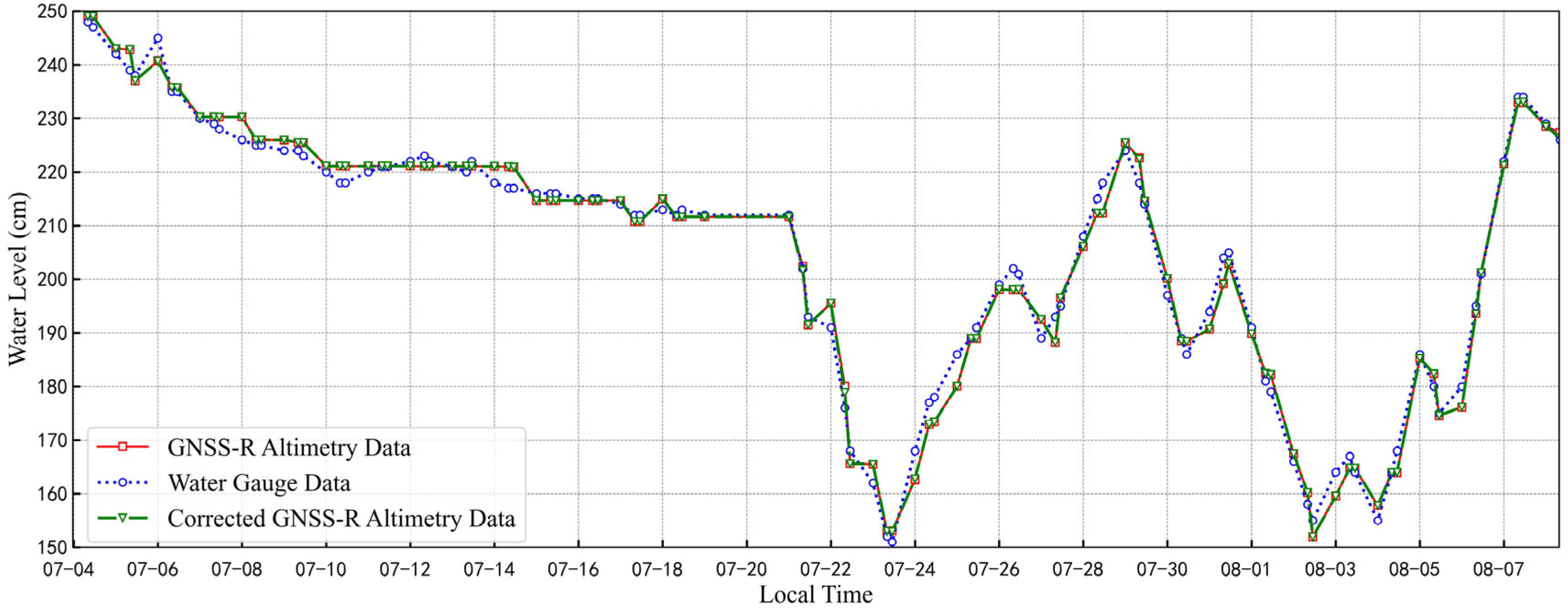
4.1. Variation of Water Surface Height
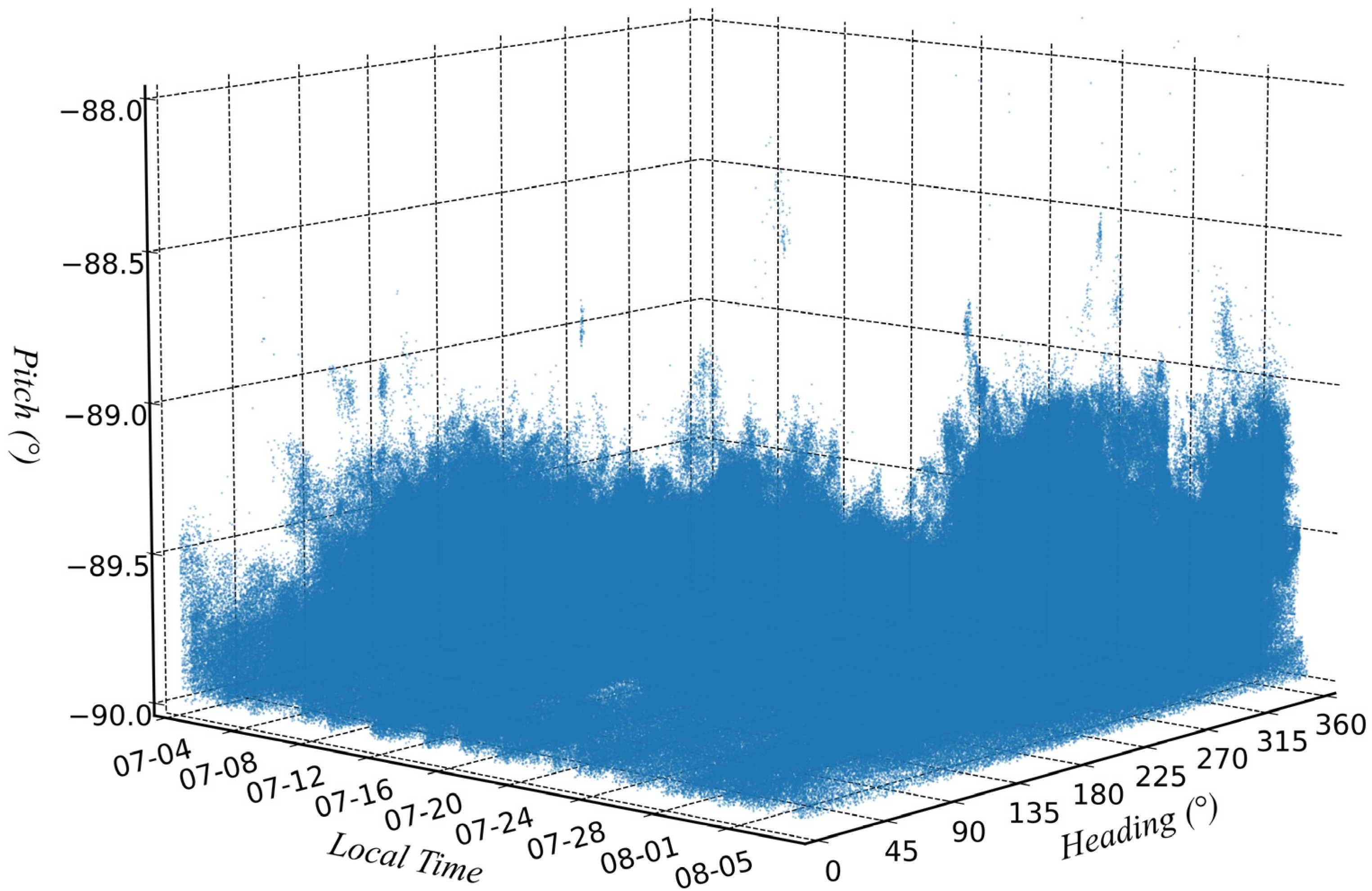
4.2. Variation of Attitude Angle
5. Discussion
Author Contributions
Funding
Data Availability Statement
Acknowledgments
Conflicts of Interest
References
- Zhu, D.; Li, H.; Wang, X. Application Prospects of GNSS Remote Sensing Technique in the Development of Smart Water Conservancy. Water Resour. Hydropower Eng. 2022, 15, 40. [Google Scholar]
- Yang, D.; Zhang, Q. GNSS Reflected Signal Processing: Fundamentals and Applications; Publishing House of Electronic Industry: Beijing, China, 2012. [Google Scholar]
- Foti, G.; Gommenginger, C.; Jales, P.; Unwin, M.; Shaw, A.; Robertson, C.; Rosello, J. Spaceborne gnss reflectometry for ocean winds: First results from the uk techdemosat-1 mission. Geophys. Res. Lett. 2015, 42, 5435–5441. [Google Scholar] [CrossRef]
- Clarizia, M.-P.; Ruf, C.; Cipollini, P.; Zuffada, C. First spaceborne observation of sea surface heightusing GPS-Reflectometry. AGU Geophys. Res. Lett. 2016, 43, 767–774. [Google Scholar] [CrossRef]
- Fabra, F. GNSS-R as A Source of Opportunity for Remote Sensing of the Cryosphere. Ph.D. Thesis, Universitat Politècnica de Catalunya, Barcelona, Spain, 2014. [Google Scholar]
- Chew, C.; Shah, R.; Zuffada, C.; Hajj, G.; Masters, D.; Mannucci, A.J. Demonstrating soil moisture remote sensing with observations from the UK TechDemoSat-1 satellite mission. Geophys. Res. Lett. 2016, 43, 3317–3324. [Google Scholar] [CrossRef]
- Zhongmin, M.; Shuangcheng, Z.; Qi, L.; Guanwen, H.; Qiancheng, K.; Jilun, P. Monitoring water level change of the Yellow River by universal GPS receivers. Nanjing Xinxi Gongcheng Daxue Xuebao 2021, 13, 187–193. [Google Scholar]
- Martín-Neira, M. A Passive reflectometry and interferometry system (PARIS): Application to ocean altimetry. ESA J. 1993, 17, 331–335. [Google Scholar]
- Anderson, K.D. Determination of water level and tides using interferometric observations of GPS signals. J. Atmos. Ocean. Technol. 2000, 17, 1118–1127. [Google Scholar] [CrossRef]
- Martin-Neira, M.; Caparrini, M.; Font-Rossello, J.; Lannelongue, S.; Vallmitjana, C. The PARIS concept: An experimental demonstration of sea surface altimetry using GPS reflected signals. IEEE Trans. Geosci. Remote Sens. 2001, 39, 142–150. [Google Scholar] [CrossRef]
- Ruffini, G.; Caparrini, M.; Ruffini, L. PARIS Altimetry with L1 Frequency Data from the Bridge 2 Experiment. arXiv 2002, arXiv:0212055. [Google Scholar]
- Wang, X.; He, X.; Zhang, Q. Evaluation and combination of quad-constellation multi-GNSS multipath reflectometry applied to sea level retrieval. Remote Sens. Environ. 2019, 231, 111229. [Google Scholar] [CrossRef]
- Xu, L.; Wan, W.; Chen, X.; Zhu, S.; Liu, B.; Hong, Y. Spaceborne GNSS-R Observation of Global Lake Level: First Results from the TechDemoSat-1 Mission. Remote Sens. 2019, 11, 1438. [Google Scholar] [CrossRef]
- Ha, M.C. Evolution of Soil Moisture and Analysis of Fluvial Altimetry Using GNSS-R. Ph.D. Thesis, Université Paul Sabatier-Toulouse III, Toulouse, France, 2018. [Google Scholar]
- Song, M.; He, X.; Wang, X.; Zhou, Y.; Xu, X. Study on the quality control for periodogram in the determination of water level using the GNSS-IR technique. Sensors 2019, 19, 4524. [Google Scholar] [CrossRef]
- Gao, F.; Xu, T.; Wang, N.; He, Y.; Luo, X. A shipborne experiment using a dual-antenna reflectometry system for GPS/BDS code delay measurements. J. Geod. 2020, 94, 88. [Google Scholar] [CrossRef]
- Semmling, M. Altimetric Monitoring of Disko Bay Using Interferometric GNSS Observations on L1 and L2. Ph.D. Thesis, Deutsches GeoForschungsZentrum GFZ, Potsdam, Germany, 2012; 136p. [Google Scholar]
- Larson, K.M.; Löfgren, J.S.; Haas, R. Coastal sea level measurements using a single geodetic GPS receiver. Adv. Space Res. 2013, 51, 1301–1310. [Google Scholar] [CrossRef]
- Löfgren, J.S.; Haas, R.; Scherneck, H.G. Sea level time series and ocean tide analysis from multipath signals at five GPS sites in different parts of the world. J. Geodyn. 2014, 80, 66–80. [Google Scholar] [CrossRef]
- Larson, K.M.; Ray, R.D.; Williams, S.D.P. A 10-year comparison of water levels measured with a geodetic GPS receiver versus a conventional tide gauge. J. Atmos. Ocean. Technol. 2017, 34, 295–307. [Google Scholar] [CrossRef]
- Wang, N.; Xu, T.; Gao, F.; Xu, G. Sea level estimation based on GNSS dual-frequency carrier phase linear combinations and SNR. Remote Sens. 2018, 10, 470. [Google Scholar] [CrossRef]
- Wang, X.; He, X.; Xiao, R.; Song, M.; Jia, D. Millimeter to centimeter scale precision water-level monitoring using GNSS reflectometry: Application to the South-to-North Water Diversion Project, China. Remote Sens. Environ. 2021, 265, 112645. [Google Scholar] [CrossRef]
- Wang, F.; Zhang, B.; Yang, D.; Xing, J.; Zhang, G.; Yang, L. Four-Channel Interference of Dual-Antenna GNSS Reflectometry and Water Level Observation. IEEE Geosci. Remote Sens. Lett. 2021, 19, 8019305. [Google Scholar] [CrossRef]
- Martín-Neira, M.; Colmenarejo, P.; Ruffini, G.; Serra, C. Altimetry precision of 1 cm over a pond using the wide-lane carrier phase of GPS reflected signals. Can. J. Remote Sens. 2002, 28, 394–403. [Google Scholar] [CrossRef]
- Löfgren, J.S.; Haas, R. Sea Level Measurements Using Multi-Frequency GPS and GLONASS Observations. EURASIP J. Adv. Signal Process. 2014, 2014, 50. [Google Scholar] [CrossRef]
- Liu, W.; Beckheinrich, J.; Semmling, M.; Ramatschi, M.; Vey, S.; Wickert, J.; Hobiger, T.; Haas, R. Coastal Sea-Level Measurements Based on GNSS-R Phase Altimetry: A Case Study at the Onsala Space Observatory, Sweden. IEEE Trans. Geosci. Remote Sens. 2017, 55, 5625–5636. [Google Scholar] [CrossRef]
- Fabra, F.; Cardellach, E.; Rius, A.; Ribo, S.; Oliveras, S.; Nogués-Correig, O.; Rivas, M.B.; Semmling, M.; D’Addio, S. Phase altimetry with dual polarization GNSS-R over sea ice. IEEE Trans. Geosci. Remote Sens. 2011, 50, 2112–2121. [Google Scholar] [CrossRef]
- He, Y.; Gao, F.; Xu, T.; Meng, X.; Wang, N. Coastal altimetry using interferometric phase from GEO satellite in quasi-zenith satellite system. IEEE Geosci. Remote Sens. Lett. 2021, 19, 3002505. [Google Scholar] [CrossRef]
- Kucwaj, J.C.; Reboul, S.; Stienne, G.; Choquel, J.B.; Benjelloun, M. Circular Regression Applied to GNSS-R Phase Altimetry. Remote Sens. 2017, 9, 651. [Google Scholar] [CrossRef]
- Bao, L.F.; Wang, N.Z.; Gao, F. Improvement of Data Precision and Spatial Resolution of cGNSS-R Altimetry Using Improved Device with External Atomic Clock. IEEE Geosci. Remote Sens. 2016, 13, 207–211. [Google Scholar] [CrossRef]
- Zhao, L.; Li, N.; Li, L.; Zhang, Y.; Chun, C. Real-Time GNSS-Based Attitude Determination in the Measurement Domain. Sensors 2017, 17, 296. [Google Scholar] [CrossRef]
- Wang, N.Z.; Bao, L.F.; Gao, F. Improved Water Level Retrieval from Epoch-by-Epoch Single and Double Difference GNSS-R Algorithms. Acta Geod. Er Cartogr. Sinica. 2016, 45, 795–802. [Google Scholar]
- Rius, A.; Nogués-Correig, O.; Ribó, S.; Cardellach, E.; Oliveras, S.; Valencia, E.; Park, H.; Tarongi, J.M.; Camps, A.; van der Marel, H.; et al. Altimetry with GNSS-R interferometry: First proof of concept experiment. GPS Solut. 2012, 16, 231–241. [Google Scholar] [CrossRef]
- Masters, D. Surface Remote Sensing Applications of GNSS Bistatic Radar: Soil Moisture and Aircraft Altimetry; University of Colorado: Boulder, CO, USA, 2004. [Google Scholar]
- Kaplan, E. Understanding GPS—Principles and Applications, 2nd ed.; Artech House: Norwood, MA, USA, 2005. [Google Scholar]
- Teunissen, P.J.G. An Optimality Property of the Integer Least-Squares Estimator. J. Geod. 1999, 73, 587–593. [Google Scholar] [CrossRef]
- Xu, G.; Xu, Y. Applications of GPS Theory and Algorithms. In GPS; Springer: Berlin/Heidelberg, Germany, 2016. [Google Scholar]
- Teunissen, P.J.G.; Montenbruck, O. Springer Handbook of Global Navigation Satellite Systems; Springer International Publishing: Cham, Switzerland, 2017. [Google Scholar]
- Frei, E.; Beutler, G. Rapid static positioning based on the fast ambiguity resolution approach ‘FARA’ theory and first results. Manuscr. Geod. 1990, 15, 325–356. [Google Scholar]
- Euler, H.-J.; Schaffrin, B. On a Measure for the Discernibility between Different Ambiguity Solutions in the Static-Kinematic GPS-Mode. In International Association of Geodesy Symposia; Springer: Berlin/Heidelberg, Germany, 1991; Volume 107, pp. 285–295. [Google Scholar]
- Tiberius, C.C.; De Jonge, P. Fast positioning using the LAMBDA method. In Proceedings of the International Symposium on Differential Satellite Navigation Systems, Bergen, Norway, 24–28 April 1995; pp. 24–28. [Google Scholar]
- Han, S. Quality-control issues relating to instantaneous ambiguity resolution for real-time GPS kinematic positioning. J. Geodesy 1997, 71, 351–361. [Google Scholar] [CrossRef]
- Song, F. Research on GNSS Integer Ambiguity Estimation Methods. Ph.D. Thesis, China University of Mining & Technology, Beijing, China, 2016. [Google Scholar]
- Zhang, Y.; Tian, L.; Meng, W.; Gu, Q.; Han, Y.; Hong, Z. Feasibility of code-level altimetry using coastal BeiDou reflection (BeiDou-R) setups. IEEE J. Stars 2015, 8, 4130–4140. [Google Scholar] [CrossRef]
- Medina, D.; Heßelbarth, A.; Büscher, R.; Ziebold, R.; García, J. On the Kalman filtering formulation for RTK joint positioning and attitude quaternion determination. In Proceedings of the 2018 IEEE/ION Position, Location and Navigation Symposium (PLANS), Monterey, CA, USA, 23–26 April 2018; pp. 597–604. [Google Scholar]
- Lau, L.; Cross, P. Development and testing of a new ray-tracing approach to GNSS carrier-phase multipath modelling. J. Geodesy 2007, 81, 713–732. [Google Scholar] [CrossRef]


| Types of Antennas | RHCP Antenna | LHCP Antenna |
|---|---|---|
| Operating temperature | −40 °C~+70 °C | −40 °C~+70 °C |
| Antenna gain | 40 ± 2 dB | 40 ± 2 dB |
| Working frequency | BDS B1/B2/B3 | BDS B1/B2/B3 |
| GPS L1/L2/L5 | GPS L1/L2/L5 | |
| GLONASS L1/L2 | GLONASS L1/L2 | |
| GALILEO E1/E5a/E5b | GALILEO E1/E5a/E5b | |
| L-Band | L-Band | |
| SBAS | SBAS | |
| Phase center error | ±2 mm | ±2 mm |
| Weight | ≤500 g | ≤500 g |
| Size | Φ147 × 67.7 | Φ147 × 67.7 |
Disclaimer/Publisher’s Note: The statements, opinions and data contained in all publications are solely those of the individual author(s) and contributor(s) and not of MDPI and/or the editor(s). MDPI and/or the editor(s) disclaim responsibility for any injury to people or property resulting from any ideas, methods, instructions or products referred to in the content. |
© 2023 by the authors. Licensee MDPI, Basel, Switzerland. This article is an open access article distributed under the terms and conditions of the Creative Commons Attribution (CC BY) license (https://creativecommons.org/licenses/by/4.0/).
Share and Cite
Zhang, P.; Pang, Z.; Lu, J.; Jiang, W.; Sun, M. Real-Time Water Level Monitoring Based on GNSS Dual-Antenna Attitude Measurement. Remote Sens. 2023, 15, 3119. https://doi.org/10.3390/rs15123119
Zhang P, Pang Z, Lu J, Jiang W, Sun M. Real-Time Water Level Monitoring Based on GNSS Dual-Antenna Attitude Measurement. Remote Sensing. 2023; 15(12):3119. https://doi.org/10.3390/rs15123119
Chicago/Turabian StyleZhang, Pengjie, Zhiguo Pang, Jingxuan Lu, Wei Jiang, and Minghan Sun. 2023. "Real-Time Water Level Monitoring Based on GNSS Dual-Antenna Attitude Measurement" Remote Sensing 15, no. 12: 3119. https://doi.org/10.3390/rs15123119
APA StyleZhang, P., Pang, Z., Lu, J., Jiang, W., & Sun, M. (2023). Real-Time Water Level Monitoring Based on GNSS Dual-Antenna Attitude Measurement. Remote Sensing, 15(12), 3119. https://doi.org/10.3390/rs15123119