Removing Time Dispersion from Elastic Wave Modeling with the pix2pix Algorithm Based on cGAN

Abstract

The finite-difference (FD) method is one of the most commonly used numerical methods for elastic wave modeling. However, due to the difference approximation of the derivative, the time dispersion phenomenon cannot be avoided. This paper proposes the use of pix2pix algorithm based on a conditional generative adversarial network (cGAN) for removing time dispersion from elastic FD modeling. Firstly, we analyze the time dispersion of elastic wave FD modeling. Then, we discuss the pix2pix algorithm based on cGAN, improve the loss function of the pix2pix algorithm by introducing a Sobel operator, and analyze the parameter selection of the network model for the pix2pix algorithm. Finally, we verify the feasibility and effectiveness of the pix2pix algorithm in removing time dispersion from elastic wave FD modeling through testing some model simulation data.

1. Introduction

The numerical computation of seismic wave equations is an important step in seismic modeling, reverse time migration, and full waveform inversion [1]. The computational accuracy of the numerical solution may affect the quality of imaging and inversion [2]. The common numerical solution methods for the wave equation include the finite-difference (FD) method [3], finite element method [4], pseudo-spectral method [5], and so on. The FD method has the advantages of simple implementation, fast calculation and easy parallelism, making it widely used in the solution of seismic wave equations [6,7]. However, the FD method approximates the time derivative by using a differential format, which unavoidably generates numerical errors known as time dispersion. Reducing the time dispersion produced by the FD method has considerable practical significance for forward modeling.

According to the derivation process of the FD method, using a smaller time step and higher-order time derivative difference approximation can mitigate the time dispersion artifacts [8], but this method requires significant computational resources. Tal-Ezer [9] proposed the rapid expansion method to reduce time dispersion. Ren et al. [10] extended the Lax–Wendroff method for suppressing space dispersion and enabled it to be used for eliminating time dispersion. Stork [11] pointed out that time dispersion is independent of the velocity model and grid settings and can be removed after propagation. Dai et al. [12] derived the analytical form of the time dispersion error, and designed a post-propagation filter to implement time dispersion suppression. Wang and Xu [13] developed a method for suppressing time dispersion by defining a time dispersion conversion operator and its inverse operator, and then used the inverse operator to overcome time dispersion. Li et al. [14] proved that improving the accuracy of time derivative differences can significantly improve the quality of forward modeling, and designed two types of filters to alleviate time dispersion by comparing waveforms. Koene et al. [15] achieved the conversion of differential solutions and numerical solutions by modifying the source function in the frequency domain. Similarly, Xu et al. [16] and Amundsen and Pedersen [17] designed different types of filters for suppressing time dispersion after propagation. However, such methods often introduce the summation of series or convolutional calculations in the design of filters, resulting in large computational complexity and potential secondary errors.

With the popularization of deep learning algorithms in the field of geophysical applications [18], some artificial intelligence algorithms have been applied to overcome numerical dispersion generated by the FD method. Moseley et al. [19] used the WaveNet to quickly simulate seismic wave propagation in complex media. Wei and Fu [20] and Rasht-Behesht et al. [21] used a physical information neural network (PINN) to obtain high-accuracy seismic wavefield simulation data. Kaur et al. [22] used cycleGAN to overcome space dispersion caused by FD method. Han et al. [23] proposed a semi-supervised neural network to eliminate time dispersion. Both of these methods involve complex neural networks, which require a large amount of time for training. Siahkoohi et al. [24] used transfer learning to suppress numerical dispersion. Gadylshin et al. [25] designed the numerical dispersion mitigation network (NDM-NET) to alleviate numerical dispersion in forward modeling for seismic waves. This method focuses on obtaining single seismic records but does not consider the propagation process of seismic waves.

In this paper, we propose the use of the pix2pix algorithm based on conditional generative adversarial network (cGAN) to remove time dispersion from elastic FD modeling. The pix2pix algorithm has a simple network structure and fast convergence rate. First, we analyze the time dispersion from elastic wave FD modeling, and then discuss the pix2pix algorithm based on cGAN. To stabilize the quality of generative result, the Sobel operator is introduced into the loss function of the pix2pix algorithm. We also analyze the problem of selecting parameters of the network in the pix2pix algorithm. Finally, we verify the feasibility and effectiveness of the pix2pix algorithm in removing time dispersion of elastic wave FD modeling through testing several model simulation data.

2. Theory and Method

2.1. Time Dispersion Analysis

The displacement–stress relations of elastic wave equations in isotropic medium are given by [26]

$$\left\{\begin{array}{l}\rho \frac{{\partial }^2{u}_x}{\partial t^2}=\frac{\partial {\tau }_{xx}}{\partial x}+\frac{\partial {\tau }_{xx}}{\partial z}\\ \rho \frac{{\partial }^2{u}_z}{\partial t^2}=\frac{\partial {\tau }_{xz}}{\partial x}+\frac{\partial {\tau }_{zz}}{\partial z}\\ {\tau }_{xx}=\left(\lambda +2\mu \right)\frac{\partial u_x}{\partial x}+\lambda \frac{\partial u_z}{\partial z}\\ {\tau }_{zz}=\left(\lambda +2\mu \right)\frac{\partial u_z}{\partial z}+\lambda \frac{\partial u_x}{\partial x}\\ {\tau }_{xz}=\mu \left(\frac{\partial u_x}{\partial z}+\frac{\partial u_z}{\partial x}\right)\end{array}\right.$$

(1)

where ρ is the density, t is the propagation time, x and z are the space coordinates, (u_x, u_z) is the displacement vector, (τ_xx, τ_xz, τ_zz) is the stress vector, λ and μ are Lamé coefficients. λ = v_p²ρ − 2v_s²ρ, μ = v_s²ρ, where v_p is the P-wave velocity and v_s is the S-wave velocity.

The general wave equation can be described by [13]

$$\frac{{\partial }^{2}u}{\partial t^2}-Lu=0,$$

(2)

where u is the displacement vector and L is the elastic potential term.

When we use the second order difference to approximate the time derivative of the wave equation, the difference solution of the wave equation [27] is

$$v^2{\nabla }^2{u}^n\left(i,j\right)=\frac{1}{\Delta t^2}\left[u^{n+1}\left(i,j\right)-2u^n\left(i,j\right)\right.\left.+u^{n-1}\left(i,j\right)\right],$$

(3)

where v is the velocity, (i, j) represents the spatial locations, n is the discrete time,${\nabla }^2$ is the Laplace operator in the space, and Δt is the time step.

Assuming homogeneous medium, we transfer Equation (3) into the wavenumbers–time domain

$$-v^2{k}^2{\tilde{u}}^n=\frac{1}{\Delta t^2}\left[{\tilde{u}}^{n+1}-2{\tilde{u}}^n+{\tilde{u}}^{n-1}\right],$$

(4)

where $\tilde{u}$ is the wavefield value in the wavenumbers domain and k is the wavenumbers.

In fact, the analytical expression of the wave equation in the wavenumbers domain is [28]

$${\tilde{u}}^{n+1}={\tilde{u}}^n{e}^{-i\omega \Delta t},$$

(5)

where ω is the angular frequency. Substituting Equation (5) into Equation (4), we get

$$v^2=\frac{2\left(1-\cos \left(\omega \Delta t\right)\right)}{\Delta t^2{k}^2}.$$

(6)

By comparing the definition of phase velocity with Equation (6), we obtain the relationship between time dispersion error and frequency, propagation time, and time step when using the second-order accuracy differential approximation for the time derivative

$${\phi }^{2nd}=\left(1-\frac{\sqrt{2-2\cos \left(\omega \Delta t\right)}}{\omega \Delta t}\right)\omega t.$$

(7)

Similarly, we obtain the expression when using the fourth-order accuracy differential approximation for the time derivative

$${\phi }^{4th}=\left(1-\frac{\sqrt{\frac{5}{2}-\frac{8}{3}\cos \left(\omega \Delta t\right)+\frac{1}{6}\cos \left(2\omega \Delta t\right)}}{\omega \Delta t}\right)\omega t.$$

(8)

Figure 1 illustrates the variation curve of time dispersion error with the difference order of time derivative, time step, and propagation time. It can be seen from the figure that increasing the difference order of time derivative and reducing the time step can effectively alleviate time dispersion.

The relationship between differential solutions and analytical solution of wave equations can be written as [15].

$$\frac{{\partial }^2{u}_f}{\partial t^2}={\mathcal{F}}^{-1}\left[\frac{1}{{\theta }^2}\mathcal{F}\left[L{u}_e+f\right]\right],$$

(9)

where $\mathcal{F}$ and ${\mathcal{F}}^{-1}$ are the Fourier transform operator and inverse Fourier transform operator, u_f is the differential solution, u_e is the exact solution, θ is a coefficient up to the order of differential approximation, and f is the source function. Through Equation (9), different differential order solutions and exact solutions can be transformed into each other.

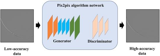
2.2. The Improvement of pix2pix Algorithm Based on cGAN

A generative adversarial network (GAN) [29] is a type of neural network architecture that uses random noise series to generate designated types of data. The generative adversarial network consists of a generator model and a discriminator model. During the iterative training process, the random noise will be used as the input for the generator model, and the training set will be used as the input of the discriminator model. The generator model needs to improve the quality of generative data to be sufficiently similar to the training set, while the discriminator model needs to enhance its ability to judge the source of data. The two compete against each other, ultimately achieving the goal of generating high-quality data. However, due to the high freedom of the generative adversarial network, the training process is prone to instability, gradient explosion, gradient vanishing and mode collapse [30], etc., during training, which can lead to the generative results deviating from the expected output. The cGAN [31] is a variant of the generative adversarial network that introduces additional data as conditions for the generator model and discriminator model. This can make the generator model and discriminator model more targeted and more stable in generating expected output data. Pix2pix [32] and cycleGAN [33] are two generative adversarial networks that use the idea of cGAN but in order to image style converting. They require the introduction of paired data as inputs, where the data are divided into original data and target data. Original data will be used as the input of the generator model, while target data together with original data will be used as the input of the discriminator model for training. The ultimate goal is to achieve functionality of converting one data type to the other data type. The main difference between pix2pix and cycleGAN is that cycleGAN only requires two groups of data, while pix2pix requires a one-to-one pairing of data. This relaxation of the requirements will lead to a more complex network structure and a longer training time cost in cycleGAN. However, in practice, the wavefield data can be matched by timestamp values. As a result, using pix2pix is a better choice. Figure 2 shows the training process for the pix2pix algorithm in removing time dispersion. Pix2pix’s input data are divided into original data and target data to limit the freedom of the network.

2.2.1. Loss Function

The loss function of pix2pix algorithm is defined as [32]

$${\mathcal{L}}_{pix2pix}\left(G,D\right)=\arg \underset{G}{\min } \underset{D}{\max }\left\{{\mathcal{L}}_{cGAN}\left(G,D\right)+{\lambda }_{l_1}{\mathcal{L}}_{l_1}\left(G\right)\right\},$$

(10)

where

$$\left\{\begin{array}{l}{\mathcal{L}}_{cGAN}\left(G,D\right)=E_{y_o,y_t}\left[\log \left(D\left(y_o,y_t\right)\right)\right]+E_{y_o}\left[\log \left(1-D\left(y_o,G(y_o\right)\right)\right]\\ {\mathcal{L}}_{l_1}\left(G\right)=E_{y_o,y_t}\left[{‖y_t-G\left(y_o\right)‖}_1\right]\end{array}\right.,$$

(11)

where G is the generator, D is the discriminator, ${\lambda }_{l_1}$ is the weight of l₁-norm, y_o is the original data, y_t is the target data, and E is the mean operator.

Training the discriminator will fix the current generator, and if the input data are from target data, the discriminator’s output will be more biased towards 1 or towards 0. Similarly, training the generator requires fixing the current discriminator. When the generator’s output is more similar to the target data, the loss function value will be smaller. Through iterative training, when the entire network converges, the generator can achieve the function of mapping the original data to the target data. In contrast, if the generator model is not limited by any conditions, due to the high freedom of high-dimensional data, it can diverge more easily. Therefore, constraints need to be added to the generator model to limit its output. The traditional pix2pix algorithm uses l₁-norm as constraints instead of l₂-norm [34]. The reason is that the smoothness property of l₂-norms can lead to the Gaussian blurring in the generative results [35].

However, Figure 3 displays generative snapshots with different loss functions. When the l₁-norm is only used to constrain the generator, the generative results still have two problems: one is the large area of block errors that should have been zero; the other is the speckle errors near vibrating regions. These errors are all boundary errors. To try to solve this problem, we introduce the Sobel operator. The Sobel operator [36] can obtain the first-order gradient value of a digital image, which is typically used in edge detection. It is one of the most commonly used edge detection algorithms in cases where accuracy requirements are not high. Figure 4 shows the horizontal and vertical convolution kernels of yjr Sobel operator. The calculation rule for the Sobel operator is to perform horizontal and vertical convolutions of the input image array with the Sobel kernel, and then threshold the resulting pixel gray value to determine edge information. The specific calculation formula for the Sobel operator is as follows:

$$\mathrm{S}=\sqrt{{\left({\mathrm{S}}_x\ast \mathrm{A}\right)}^2+{\left({\mathrm{S}}_y\ast \mathrm{A}\right)}^2},$$

(12)

where S_x and S_y are the Sobel horizontal and vertical convolution kernels, respectively, A is the input data, and * is the convolution operator.

2.2.2. Generator

The generator in the pix2pix algorithm can use either the U-Net structure or the Encode–Decode structure. Figure 5 displays the frameworks of the U-Net structure and the Encode–Decode structure. The U-Net structure is composed of four modules: the initialization module, the recovery module, and several up-sampling and down-sampling modules. The corresponding up-sampling and down-sampling modules are connected by a skip connection. The Encode–Decode structure is composed of five modules: the initialization module, the recovery module, several encoding modules, decoding modules, and residual modules. Unlike the U-Net structure, the encoding modules and decoding modules are not directly connected, but are connected by several residual modules in the middle layer.

Figure 6 shows the generative results with the U-Net or Encode–Decode structures as generators under the same parameters. It can be clearly seen that both types of generators can effectively remove the time dispersion produced by FD methods. However, the results generated by the U-Net network have some Gaussian blurring errors near the wavefront, while the results generated by the Encode–Decode network are almost identical to the results generated by high-order approximations. From the perspective of generating results, the Encode–Decode network is more accurate. From the perspective of network parameters, the number of parameters in the U-Net network is 217,996,993, while the number of parameters in the Encode-Decode network is 407,265. Therefore, the Encode–Decode network is more suitable for generating results.

2.2.3. Discriminator

The output of discriminator in traditional generative adversarial networks is usually a single value between 0 and 1 as an indicator to determine the data source. The closer the output value approaches 0, the more likely it is that the discriminator believes the result is generated by the generator. Conversely, the discriminator believes that the result is more likely to be real data. The discriminator of the pix2pix algorithm consists of several consecutive convolutional layers, which ultimately outputs a k × k square matrix, using the mean value of the square matrix as the judgment criterion. This judgment method is equivalent to partitioning the image into k × k patches, and the discriminator evaluates each block’s source separately, and finally selects the data source based on the judgment of results of all blocks. This method has two advantages: firstly, it can avoid simple averaging of different data patches; secondly, the discriminator outputs k × k small patches instead of a single value, which can effectively reduce the number of layers and parameters of the network, reduce the complexity of the network, and speed up training.

The value of k is usually 2 to the nth, which simplifies the structure of the discriminators. The smaller the n is, the deeper the discriminator layers are and the longer the training time required. Figure 7 illustrates the variation of loss function values with iteration number under different k-values. From the figure, it can be seen that the overall loss function decreases relatively quickly, but when k-values are 16, 64, and 128, there are some fluctuations in the loss function after stability, which may lead to falling into a local maximum and unstable generative results. When k-values are 8 or 32, there is no such problem, but when the k-value is 32, the network structure is more concise and training speed is faster. Therefore, the output size of the discriminator is ultimately selected as 32 × 32.

2.3. Training Set Size

The training set size will affect the final generative results. When the training set size is too small, the network may struggle to learn the mapping relationships, resulting in distorted results. However, if the training set size is too large, it may lead to overfitting, resulting in inaccurate results. We define the “Average Patch Score” (APS) as the mean absolute value of the differences between each discriminator output patch and the expected output patch. A lower APS indicates a more accurate generated result.

Table 1. APS of generative result of different sample size.

Number of Samples	100	200	300	400	500
APS (100 epochs)	2.53	2.62	2.31	2.55	2.64
APS (200 epochs)	1.82	2.37	2.06	2.01	2.75
APS (300 epochs)	2.42	2.04	2.07	1.62	2.41
APS (400 epochs)	2.06	2.29	1.98	1.59	2.37

displays the APS of different sample sizes. When using smaller sample sizes of 100 and 200, it is difficult for the network to learn the data features and thus it generates large errors, with APS values not improving significantly with increasing iterations. When using sample sizes of 500, APS shows oscillations rather than a decrease. Using sample sizes of 300 and 400 are more effective; specifically, 400 is the best.

3. Numerical Experiments

3.1. Homogeneous Model

To test the pix2pix algorithm, we design a homogeneous model with the size of 5110 m × 5110 m. The grid spacing is 10 m × 10 m and the P-wave velocity, S-wave velocity, and density are 2200 m/s, 1600 m/s, and 1900 kg/m³, respectively. The source uses the Ricker wavelet with a principal frequency of 25 Hz. The time step for the original data with time dispersion is 0.002 s, and the time derivative is approximated using the 2nd-order difference [26]. The time step for the target data with low time dispersion is 0.001 s, and the time derivative is approximated using a fourth-order difference. Both used 20th-order FD on spatial derivatives. The boundary condition is implemented by the perfectly matched layer (PML) boundary condition [37].

In terms of neural network models, the generator uses the 19-layer Encode–Decode structure, which is divided into initializing modules, 3 up-sampling modules, 11 residual modules, 3 down-sampling modules, and recovery modules. The discriminator uses a continuous five-layer convolutional layer, which outputs a 32 × 32 square matrix as its final output. The training set has 400 samples, with the l₁-norm weight value being 30, the Sobel loss weight value being 10, and the learning rate being 0.001.

Figure 8 shows the horizontal component of modeling snapshots at 1.2 s using the above parameter settings in the homogeneous model and the source located at (100 m, 100 m). The generative result is trained for 400 rounds. In this figure, the wavefield exhibits severe time dispersion, blurred edges, and low resolution when using low-order differences. After using high-order difference, the time dispersion phenomenon is significantly reduced. The generative result using the pix2pix algorithm is almost identical to that obtained from high-order difference, and the blurred wave fronts caused by time dispersion are completely removed, making the energy more concentrated.

Figure 9 displays the single-trace record at receiver x = 2560 m. In this figure, the vibration curve obtained from the low-order difference shows an obvious wave motion that occurs earlier than time, while the vibration curve corrected by the pix2pix algorithm is similar to that obtained from the high-order difference, removing the wave motion that occurs earlier than time, alleviating the time dispersion.

3.2. Two-Layer Model

In order to further test the applicability of the pix2pix algorithm, we design a two-layer model with the size of 5110 m × 5110 m, and the mesh spacing of 10 m × 10 m. Figure 10 shows the parameters of the two-layer model. In this model, the upper layer has the P-wave velocity of 2000 m/s, the S-wave velocity of 1600 m/s, the density of 1900 kg/m³, and the depth of 3500 m. The lower layer has the P-wave velocity of 2200 m/s, the S-wave velocity of 1800 m/s, and the density of 2300 kg/m³. The source uses a 25 Hz Ricker wave. The data source, computation method, and the parameters of the pix2pix network are consistent with those in the homogeneous model.

Figure 11 shows the horizontal component of modeling snapshots at 1.6 s using the above parameter settings in the two-layer model and the source is located at (4000 m, 100 m). The generative result is trained for 400 rounds. When using low-order difference, the time dispersion in the two-layer model is more pronounced, resulting in blurred edges and low resolution. However, using the pix2pix algorithm almost perfectly reproduces the target data obtained from high-order difference. The pix2pix algorithm generates a very clear wavefield.

Figure 12 shows the shot records in the two-layer model. The corrected records using the pix2pix algorithm clearly remove the time dispersion. Figure 12d illustrates comparison of the extracted record at point (100 m, 100 m). After using the pix2pix algorithm, we can clearly observe that the generative result effectively reduces the pre-time vibration between 1.4 s and 1.45 s.

3.3. Marmousi Model

Figure 13 shows a cropped Marmousi model, which is discretized into 512 × 512 grids at the space 10 m × 10 m. The source uses the Ricker wavelet of 25 Hz. The acquisition of training set and the setting of pix2pix algorithm is consistent with those used in the previous section.

Figure 14 shows the horizontal component of modeling snapshots at 1.5 s using the above parameter settings in the cropped Marmousi model with the source is located at (5000 m, 100 m). The generative result is trained for 400 rounds. In this figure, the low-order difference data show serious time dispersion, a chaotic wavefront, and scattered energy, while the pix2pix algorithm generated results reduces the pseudo-wavefront and effectively removes the time dispersion. The suppression effect on time dispersion is almost the same as that obtained by improving difference order and reducing time-step size.

Figure 15 displays single-trace records at receiver x = 3000 m. The vibration recorded using low-order difference shows a significant amount of time dispersion at 1.6–1.7 s, resulting in the appearance of oscillations. However, the vibration record revised by the pix2pix algorithm removes the pseudo-wavefront and time dispersion. The subsequent vibration curve is also similar to the high-order difference curve, indicating that the pix2pix algorithm has almost achieved the conversion function from low-order difference to high-order difference.

Figure 16 illustrates the loss function variation curve in this model. The loss decreases rapidly early in the training, which indicates that our method does not require too large training time. However, to avoid getting trapped in the local optimal solution shown in Figure 7, we moderately increase the number of training epochs, to 400.

Figure 17 illustrates the time cost to compute different numbers of shot records in the cropped Marmousi model. The time cost of our method includes three parts: using low-order approximation computation, training set preparation with training time, and using network correction. The training process requires some additional time cost; therefore, our method is not suitable when only a few records are needed. However, as the number of records increases, the time cost of our method is gradually lower than the method that directly improves the approximation accuracy. Moreover, the increase in time cost for training 400 epochs is also not noticeable.

4. Conclusions

We have presented a method that uses the pix2pix algorithm based on cGAN to remove time dispersion from elastic FD modeling. In order to reduce the training time, the Encode–Decode structure is used as the generator. The appropriate output size of discriminator is chosen, which makes the generated results more stable. Since the snapshot data have distinct boundaries, the Sobel operator is introduced into the loss function to improve the quality of the generative results. By testing in different models, the feasibility and effectiveness of the pix2pix algorithm based on cGAN to remove time dispersion from elastic FD modeling are verified. In addition, since a small training set of samples are used, the proposed is method less time-consuming.

References

1. Takougang, E.M.T.; Ali, M.Y.; Bouzidi, Y.; Bouchaala, F.; Sultan, A.A.; Mohamed, A.I. Characterization of a carbonate reservoir using elastic full-waveform inversion of vertical seismic profile data. Geophys. Prospect. 2020, 68, 1944–1957. [Google Scholar] [CrossRef]
2. Pei, Z.; Mu, Y. Numerical simulation of seismic wave propagation. Prog. Geophys. 2004, 19, 933–941. [Google Scholar]
3. Alterman, Z.; Karal, F., Jr. Propagation of elastic waves in layered media by finite difference methods. Bull. Seismol. Soc. Am. 1968, 58, 367–398. [Google Scholar]
4. Lysmer, J.; Drake, L.A. A finite element method for seismology. Methods Comput. Phys. 1972, 11, 181–216. [Google Scholar]
5. Kosloff, D.D.; Baysal, E. Forward modeling by a Fourier method. Geophysics 1982, 47, 1402–1412. [Google Scholar] [CrossRef] [Green Version]
6. Kristek, J.; Moczo, P.; Chaljub, E.; Kristekova, M. A discrete representation of a heterogeneous viscoelastic medium for the finite-difference modelling of seismic wave propagation. Geophys. J. Int. 2019, 217, 2021–2034. [Google Scholar] [CrossRef] [Green Version]
7. Matsushima, J.; Ali, M.Y.; Bouchaala, F. Propagation of waves with a wide range of frequencies in digital core samples and dynamic strain anomaly detection: Carbonate rock as a case study. Geophys. J. Int. 2021, 224, 340–354. [Google Scholar] [CrossRef]
8. Dong, G. Dispersive problem in seismic wave propagation numerical modeling. Nat. Gas Ind. 2004, 24, 53–56. [Google Scholar]
9. Tal-Ezer, H. Spectral methods in time for hyperbolic equations. SIAM J. Numer. Anal. 1986, 23, 11–26. [Google Scholar] [CrossRef] [Green Version]
10. Ren, Z.; Bao, Q.; Gu, B. Time-dispersion correction for arbitrary even-order Lax-Wendroff methods and the application on full-waveform inversionTime-dispersion correction. Geophysics 2021, 86, T361–T375. [Google Scholar] [CrossRef]
11. Stork, C. Eliminating nearly all dispersion error from FD modeling and RTM with minimal cost increase. In Proceedings of the 75th EAGE Conference & Exhibition incorporating SPE EUROPEC 2013, London, UK, 10–13 June 2013. [Google Scholar]
12. Dai, N.; Wu, W.; Liu, H. Solutions to numerical dispersion error of time FD in RTM. In SEG Technical Program Expanded Abstracts 2014; Society of Exploration Geophysicists: Houston, TX, USA, 2014; pp. 4027–4031. [Google Scholar]
13. Wang, M.; Xu, S. Finite-difference time dispersion transforms for wave propagation. Geophysics 2015, 80, WD19–WD25. [Google Scholar] [CrossRef]
14. Li, Y.E.; Wong, M.; Clapp, R. Equivalent accuracy at a fraction of the cost: Overcoming temporal dispersion. Geophysical 2016, 81, T189–T196. [Google Scholar] [CrossRef] [Green Version]
15. Koene, E.F.M.; Robertsson, J.O.A.; Broggini, F.; Andersson, F. Eliminating time dispersion from seismic wave modeling. Geophys. J. Int. 2018, 213, 169–180. [Google Scholar] [CrossRef]
16. Xu, Z.; Jiao, K.; Cheng, X.; Sun, D.; King, R.; Nichols, D.; Vigh, D. Time-dispersion filter for finite-difference modeling and reverse time migration. In Proceedings of the 2017 SEG International Exposition and Annual Meeting, Houston, TX, USA, 24–27 September 2017. [Google Scholar]
17. Amundsen, L.; Pedersen, Ø. Elimination of temporal dispersion from the finite-difference solutions of wave equations in elastic and anelastic models. Geophysics 2019, 84, T47–T58. [Google Scholar] [CrossRef]
18. Yu, S.; Ma, J. Deep learning for geophysics: Current and future trends. Rev. Geophys. 2021, 59, e2021RG000742. [Google Scholar] [CrossRef]
19. Moseley, B.; Nissen-Meyer, T.; Markham, A. Deep learning for fast simulation of seismic waves in complex media. Solid Earth 2020, 11, 1527–1549. [Google Scholar] [CrossRef]
20. Wei, W.; Fu, L.-Y. Small-data-driven fast seismic simulations for complex media using physics-informed Fourier neural operators. Geophysics 2022, 87, T435–T446. [Google Scholar] [CrossRef]
21. Rasht-Behesht, M.; Huber, C.; Shukla, K.; Karniadakis, G.E. Physics-informed neural networks (PINNs) for wave propagation and full waveform inversions. J. Geophys. Res. Solid Earth 2022, 127, e2021JB023120. [Google Scholar] [CrossRef]
22. Kaur, H.; Fomel, S.; Pham, N. Overcoming numerical dispersion of finite-difference wave extrapolation using deep learning. In Proceedings of the SEG Technical Program Expanded Abstracts 2019, San Antonio, TX, USA, 15–20 September 2019; pp. 2318–2322. [Google Scholar]
23. Han, Y.; Wu, B.; Yao, G.; Ma, X.; Wu, D. Eliminate time dispersion of seismic wavefield simulation with semi-supervised deep learning. Energies 2022, 15, 7701. [Google Scholar] [CrossRef]
24. Siahkoohi, A.; Louboutin, M.; Herrmann, F.J. The importance of transfer learning in seismic modeling and imaging. Geophysics 2019, 84, A47–A52. [Google Scholar] [CrossRef]
25. Gadylshin, K.; Vishnevsky, D.; Gadylshina, K.; Lisitsa, V. Numerical dispersion mitigation neural network for seismic modeling. Geophysics 2022, 87, T237–T249. [Google Scholar] [CrossRef]
26. Virieux, J. P-SV wave propagation in heterogeneous media: Velocity-stress finite-difference method. Geophysics 1986, 51, 889–901. [Google Scholar] [CrossRef]
27. Baysal, E.; Kosloff, D.D.; Sherwood, J.W.C. Reverse time migration. Geophysics 1983, 48, 1514–1524. [Google Scholar] [CrossRef] [Green Version]
28. Stepanishen, P.; Ebenezer, D. A joint wavenumber-time domain technique to determine the transient acoustic radiation loading on planar vibrators. J. Sound Vib. 1992, 157, 451–465. [Google Scholar] [CrossRef]
29. Goodfellow, I.; Pouget-Abadie, J.; Mirza, M.; Xu, B.; Warde-Farley, D.; Ozair, S.; Courville, A.; Bengio, Y. Generative adversarial nets. In Proceedings of the Neural Information Processing Systems 2014, Montreal, QC, Canada, 8–13 December 2014. [Google Scholar]
30. Arjovsky, M.; Bottou, L. Towards principled methods for training generative adversarial networks. arXiv 2017, arXiv:1701.04862. [Google Scholar]
31. Mirza, M.; Osindero, S. Conditional generative adversarial nets. arXiv 2014, arXiv:1411.1784. [Google Scholar]
32. Isola, P.; Zhu, J.-Y.; Zhou, T.; Efros, A.A. Image-to-image translation with conditional adversarial networks. In Proceedings of the 2017 IEEE Conference on Computer Vision and Pattern Recognition, Honolulu, HI, USA, 21–26 July 2017; pp. 1125–1134. [Google Scholar]
33. Zhu, J.Y.; Park, T.; Isola, P.; Efros, A.A. Unpaired image-to-image translation using cycle-consistent adversarial networks. In Proceedings of the IEEE International Conference on Computer Vision, Venice, Italy, 22–29 October 2017. [Google Scholar]
34. Pan, W.; Torres-Verdín, C.; Pyrcz, M.J. Stochastic pix2pix: A new machine learning method for geophysical and well conditioning of rule-based channel reservoir models. Nat. Resour. Res. 2021, 30, 1319–1345. [Google Scholar] [CrossRef]
35. Guo, L.; Song, G.; Wu, H. Complex-valued Pix2pix—Deep neural network for nonlinear electromagnetic inverse scattering. Electronics 2021, 10, 752. [Google Scholar] [CrossRef]
36. Sobel, I.; Feldman, G. A 3×3 Isotropic Gradient Operator for Image Processing. 1973. Available online: https://www.researchgate.net/publication/285159837_A_33_isotropic_gradient_operator_for_image_processing (accessed on 2 May 2023).
37. Qin, Z.; Lu, M.; Zheng, X.; Yao, Y.; Zhang, C.; Song, J. The implementation of an improved NPML absorbing boundary condition in elastic wave modeling. Appl. Geophys. 2009, 6, 113–121. [Google Scholar] [CrossRef]
Figure 1. Time dispersion with different difference order of time derivative, time step, and propagation time.
Remotesensing 15 03120 g001
Figure 2. Training process of pix2pix algorithm for removing time dispersion.
Remotesensing 15 03120 g002
Figure 3. Generative snapshots: (a) loss function only with l1-norm, (b) loss function with l1-norm and Sobel operator.
Remotesensing 15 03120 g003
Figure 4. The Sobel kernels.
Remotesensing 15 03120 g004
Figure 5. Two alternative generator structures: (a) U-Net structure, (b) Encode–Decode structure.
Remotesensing 15 03120 g005
Figure 6. Modeling snapshots with different methods: (a) snapshot modeled with 2nd-order FD on time derivatives, (b) snapshot modeled with 4th-order FD on time derivatives, (c) snapshot corrected by the network with U-Net as generator model, (d) snapshot corrected by the network with Encode–Decode as generator model.
Remotesensing 15 03120 g006
Figure 7. The loss function varies with the iteration times under different k values.
Remotesensing 15 03120 g007
Figure 8. Modeling snapshots at 1.2 s for a homogeneous model: (a) snapshot modeled with 2nd-order FD on time derivatives, (b) snapshot modeled with 4th-order FD on time derivatives, (c) snapshot corrected by the proposed method, (d) the difference between (b,c).
Remotesensing 15 03120 g008aRemotesensing 15 03120 g008b
Figure 9. Single-trace record at receiver x = 2560 m.
Remotesensing 15 03120 g009
Figure 10. Two layer model.
Remotesensing 15 03120 g010
Figure 11. Model snapshots at 1.6 s for a two-layer model: (a) snapshot modeled with 2nd-order FD on time derivatives, (b) snapshot modeled with 4th-order FD on time derivatives, (c) snapshot corrected by the proposed method, (d) the difference between (b,c).
Remotesensing 15 03120 g011
Figure 12. Modeling shot records for a two-layer model: (a) shot record modeled with 2nd-order FD on time derivatives, (b) shot record modeled with 4th-order FD on time derivatives, (c) shot record corrected by the proposed method, (d) comparison of the shot records extracted from (ac).
Remotesensing 15 03120 g012aRemotesensing 15 03120 g012b
Figure 13. The cropped Marmousi model: (a) P-wave velocity, (b) S-wave velocity, (c) density.
Remotesensing 15 03120 g013
Figure 14. Modeling snapshots at 1.5 s for a cropped Marmousi model: (a) snapshot modeled with 2nd-order FD on time derivatives, (b) snapshot modeled with 4th-order FD on time derivatives, (c) snapshot corrected by the proposed method, (d) the difference between (b,c).
Remotesensing 15 03120 g014
Figure 15. Single-trace records at receiver x = 3000 m.
Remotesensing 15 03120 g015
Figure 16. Loss function decline curve.
Remotesensing 15 03120 g016
Figure 17. The computing costs of the numerical modeling performed on the cropped Marmousi model by different methods.
Remotesensing 15 03120 g017