Algorithms and Predictors for Land Cover Classification of Polar Deserts: A Case Study Highlighting Challenges and Recommendations for Future Applications

Abstract

The use of remote sensing for developing land cover maps in the Arctic has grown considerably in the last two decades, especially for monitoring the effects of climate change. The main challenge is to link information extracted from satellite imagery to ground covers due to the fine-scale spatial heterogeneity of Arctic ecosystems. There is currently no commonly accepted methodological scheme for high-latitude land cover mapping, but the use of remote sensing in Arctic ecosystem mapping would benefit from a coordinated sharing of lessons learned and best practices. Here, we aimed to produce a highly accurate land cover map of the surroundings of the Canadian Forces Station Alert, a polar desert on the northeastern tip of Ellesmere Island (Nunavut, Canada) by testing different predictors and classifiers. To account for the effect of the bare soil background and water limitations that are omnipresent at these latitudes, we included as predictors soil-adjusted vegetation indices and several hydrological predictors related to waterbodies and snowbanks. We compared the results obtained from an ensemble classifier based on a majority voting algorithm to eight commonly used classifiers. The distance to the nearest snowbank and soil-adjusted indices were the top predictors allowing the discrimination of land cover classes in our study area. The overall accuracy of the classifiers ranged between 75 and 88%, with the ensemble classifier also yielding a high accuracy (85%) and producing less bias than the individual classifiers. Some challenges remained, such as shadows created by boulders and snow covered by soil material. We provide recommendations for further improving classification methodology in the High Arctic, which is important for the monitoring of Arctic ecosystems exposed to ongoing polar amplification.

1. Introduction

Land cover maps are among the most important products derived from remotely sensed data [1]. Land cover mapping aims to accurately identify the distribution of different types of coverings, such as vegetation, water, bare ground, rock, ice, snow, and anthropogenic infrastructure, in a particular area [2]. Due to their chemical and physical characteristics, each land cover class absorbs, reflects, and transmits electromagnetic radiation differently than other natural and anthropogenic covers, which makes remote sensing possible [3,4]. Primarily developed for forestry and environmental impact assessment, land cover maps are now important tools for multidisciplinary research and can support a wide range of applications across scales, including the design of spatially stratified studies, wildlife habitat assessment, and landscape-change detection [5,6].

With the recent advances in remote sensing technologies, including finer spatial and spectral resolution imagery and improved spatial coverage [7], land cover and vegetation maps are now being produced at a higher rate, especially for Arctic regions where there is an urgent need to monitor the effects of climate change [8]. Dramatic climate warming approximating four times the global average, known as Arctic amplification [9], coupled with the Arctic’s fragile ecological environment, has caused and will continue to cause major changes in this key region, leading to significant consequences for the earth system, such as greenhouse gas release and sea-level rise [10]. Marked changes in the Arctic have already been documented, including shifts in primary productivity, vegetation species composition, hydrological and disturbance regimes (e.g., thawing permafrost and tundra fire), as well as changes in herbivore grazing [8,11,12,13,14]. Land cover mapping thus provides a basis for the comparable and repeated monitoring of these changes over time [15], enabling the detection of potential ecosystem state changes. Applications of land cover and vegetation maps associated with climate change in the Arctic encompass the monitoring of permafrost degradation [16,17], upscaling of carbon fluxes and pools [18], the study of postfire tundra succession [19,20], grazing impact assessment [21,22], vegetation monitoring [23,24,25,26,27,28], and shore erosion evaluation [29]. Other uses of land cover maps include characterizing wildlife habitats [30,31,32], establishing the ecological monitoring of Arctic national parks [33], and estimating the human footprint due to infrastructure expansion [34].

There is still no commonly accepted methodology for high-latitude land cover mapping. Instead, a high variety of options exist in terms of sensors, classification methods and algorithms, land cover classes, and predictors. Multiple sensors with different capabilities have been used to achieve land cover classification, including high-to-coarse resolution, multispectral or hyperspectral, satellite, or airborne sensors (i.e., airplane, helicopter, or drone) [33,35,36,37]. Arctic ecosystem mapping efforts to date have applied image categorical classifications consisting of procedures for assigning each pixel or object in an image to a particular land cover class, using raster analysis or visual photo interpretation [6]. When raster analysis is chosen, the most used classification algorithms include random forests (RFs) (e.g., [1,7,38,39,40]), maximum likelihood (ML) [5,35,41], convolutional neural networks (CNNs) [42,43], support vector machines (SVMs) [44], artificial neural networks (ANNs) [42], and linear discriminant analysis (LDA) [45]. Two methods of classification are available when using raster analysis, namely supervised (classes are assigned to pixels or segments by the analyst) and unsupervised (the algorithm detects patterns in data based on the clustering of the spectral characteristics of pixels or segments) [2]. Supervised classification usually needs a sufficient number of reference points classified through extensive in situ surveys. The most accurate classifications of tundra vegetation were undertaken using supervised learning with ground-based plot surveys [46,47,48]. The Arctic land cover classes commonly include nonvegetated covers, such as snow, ice, human infrastructure, water, and bare ground (shaded areas are usually also included in nonvegetated covers), as well as vegetated covers that are stratified by community composition (e.g., [35,39,43,45,49]), plant functional types [6,20,40,50], and percent vegetation cover [51]. As for predictors, spectral bands, vegetation indices (e.g., the Normalized Difference Vegetation Index (NDVI)), soil moisture indices (e.g., the Normalized Difference Water Index (NDWI)), and terrain characteristics derived from a digital elevation model (DEM) (e.g., slope position and shape, elevation, and aspect) have often been used to achieve classification for tundra ecosystems [5,15].

Some land cover and vegetation maps covering the Arctic exist. Good examples include the Circumpolar Arctic Vegetation Map (CAVM, [52,53]), the Climate Change Initiative Land Cover (CCI-LC, [54]), the GlobeLand30 [55], and the Circumpolar Arctic Land Cover product for circa 2020 (CALC-2020, [56]). However, these maps are still spatially or thematically too coarse for many applications [57]. The spatial heterogeneity of vegetation and terrain is omnipresent in the Arctic and is driven by the small stature of tundra vegetation (occupying centimeters to a few meters of space both vertically and horizontally), the presence of small waterbodies, and the differences in microelevation due to geomorphic features, such as nonsorted circles, hummocks, low- or high-center polygons, that relate closely to substrate moisture [15,37,58,59]. Consequently, high-to-medium-resolution maps (<30 m grid cell size) are needed to represent this heterogeneity of Arctic ecosystems [60].

Most studies aiming to map vegetated and nonvegetated covers to a fine scale focused on Low Arctic rather than High Arctic ecosystems because it is logistically easier to collect field data in the Low Arctic [15]. However, there are notable differences between the Low and High Arctic, which limit the transferability of methods between these two regions. For example, vegetated cover in certain High Arctic regions is discontinuous, with extensive exposed rock and soil requiring the background reflectance to be considered to accurately classify vegetation [45,61]. In addition, Low Arctic tundras include a canopy with multiple strata and a shrub layer reaching 40 cm to 2 m high, whereas High Arctic deserts typically have one or two layers of small-stature vegetation and a prostrate dwarf shrub layer no more than 5 cm tall [61], thus making irrelevant the use of light detection and ranging (LiDAR) or 3D stereoscopy to measure the canopy structure [24,62]. Biological and climatic heterogeneity also exists within the High Arctic, especially between subzone A (polar desert), subzone B (northern tundra), and subzone C (middle tundra), the three bioclimatic subzones of the CAVM [53]. Although spatial heterogeneity is less significant in the High Arctic than in the Low Arctic, methodologies for developing land cover maps must be adapted to local and regional scales. Improved mapping and classification at the appropriate thematic level and spatial and temporal scales will significantly advance our understanding and monitoring of Arctic ecosystems.

Here, we aimed to produce a highly accurate land cover map of a large patch of polar desert surrounding the Canadian Forces Station Alert on Ellesmere Island (Nunavut, Canada) for future use in wildlife habitat assessment and ecological monitoring. This was necessary to bring the Department of National Defence of Canada into supporting the Nunavut Wildlife Act, Migratory Birds Convention Act, and Species at Risk Act. Polar deserts, bioclimatic subzone A, are the most representative landscapes of the High Arctic, encompassing 1,358,000 km² or approximately 26% of the terrestrial Arctic [63] and yet remain less studied than any other Arctic region. This case study provided us with an exceptional opportunity to test different classification algorithms (or classifiers) and predictors to accurately map land cover classes and assess the most adapted methodology for a High Arctic site. Notably, we included as predictors vegetation indices that were able to consider the effect of the soil background [64], as polar deserts are predominantly characterized by sparse vegetation on a bare soil or rocky substrate. The spectral properties of soils are known to influence the detection of sparse vegetation when using common vegetation indices, such as the NDVI and the Green Normalized Difference Vegetation Index (GNDVI) [64]. We also included hydrological predictors because water deficit is one of the most common environmental stresses limiting primary productivity in the terrestrial Arctic [65]. In addition, we tested eight popular classifiers, including the most widely used (RFs and ML) and used an ensemble classifier (EC) based on a majority voting algorithm, with each classifier having one vote and each pixel retaining the land cover class with the highest vote [66]. Combining independent classifiers through an EC is a recognized method for improving the accuracy of the model [66]. Through the evaluation of a large range of predictors and multiple commonly used algorithms, our study demonstrates how to determine the most appropriate methodology to generate an accurate map of High Arctic land cover classifications. We also provide general recommendations on themes that are common to most land cover mapping exercises. In an effort to allow replicability and facilitate the mapping of land cover classes for other Arctic sites [15], the R scripts that were used to create the land cover maps of this study are freely available on Dryad [67].

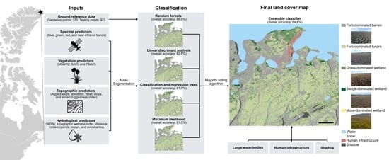
2. Materials and Methods

Our methodological workflow (Figure 1) involves four steps, each described below in its own section, namely data acquisition and extraction (Section 2.2), data preprocessing (Section 2.3), classification of land cover classes (Section 2.4), and data postprocessing (Section 2.5).

2.1. Study Area

The 170 km² study area surrounds the Canadian Forces Station Alert (82°30′N, 62°20′W), the northernmost permanently inhabited settlement on Earth, which is located on the northeastern tip of Ellesmere Island, Nunavut, Canada (Figure 2). The study area (hereafter called “Alert”) is roughly delimited by the Lincoln Sea to the north and the boundaries of Alert property in other directions. Toponymy of local landscape features appears in Desjardins et al. [68]. The entire area lies in a zone of continuous permafrost > 600 m thick, with an underlying highly calcareous bedrock, composed of argillite with greywacke in some places [69]. Alert is situated in bioclimatic subzone A of the CAVM, the coldest bioclimatic subzone in the Canadian Arctic, with an average July temperature of 3 °C [70]. This subzone is generally characterized by a polar desert landscape that is mostly barren with some lichens, biological soil crusts, and mosses, as well as vascular plant cover <5% [70]. The development of plant communities is limited by nitrogen availability that increases with soil moisture [71]. The uplands are mostly mesic or xeric and consist mainly of boulders, frost-shattered rocks, gravel, and polygonal nets of till, with very low vegetation cover growing inside soil interstices. In the lowlands where soil moisture accumulates, a more continuous vegetation cover develops, consisting primarily of grasses and sedges [72]. The sun remains under the horizon from mid-October to late February, and a 24 h sunlight period occurs from early April to early September. The growing season extends from June to August. Climate in the study area is strongly influenced by its proximity to sea ice with a mean temperature in the warmest month of approximately 3.4 °C and annual snowfall and rainfall averaging, respectively, 184.6 and 1.7 cm (corresponding to a combined water equivalent of 158 mm) [73].

2.2. Data Acquisition and Extraction

2.2.1. Ground Reference Data

We obtained ground references for seven land cover classes: forb-dominated barren, forb-dominated tundra, grass-dominated wetland, sedge-dominated wetland, moss-dominated wetland, water, and snow. The five plant communities were identified in Desjardins et al. [75] and are described in

Table 1. Description of the five plant communities, including dominant vegetation and mean percentage cover of ground, cryptogams, and vascular species groups. Adapted with permission from Desjardins et al. [75] (© 2021 The Author(s). Published by Informa UK Limited, trading as Taylor & Francis Group).

Plant Community	Dominant Vegetation	Cover (%)
		Soil/Rock	Biological Soil Crust	Lichen	Moss	Algae/ Macrofungus	Graminoid	Forb	Shrub
Forb- dominated barren	Saxifraga oppositifolia Linnaeus subsp. oppositifolia Salix arctica Pallas Mosses	88.0	0.2	1.5	1.6	0	2.1	5.6	1.8
Forb- dominated tundra	Saxifraga oppositifolia Linnaeus subsp. oppositifolia Mosses Stellaria longipes Goldie subsp. longipes	57.2	1.3	0.7	8.7	0.1	6.5	25.0	2.1
Grass- dominated wetland	Mosses Alopecurus magellanicus Lamarck Juncus biglumis Linnaeus	21.0	3.6	0.2	22.3	0.5	35.8	13.9	4.3
Sedge- dominated wetland	Eriophorum triste (Th. Fries) Hadac and Á. Löve Mosses Salix arctica Pallas	4.0	0.2	<0.1	20.5	0.1	58.2	7.6	10.3
Moss- dominated wetland	Mosses Saxifraga cernua Linnaeus Luzula nivalis (Laestadius) Sprengel	3.7	4.1	0.5	53.0	0.3	15.7	24.2	0.4

. Briefly, we conducted stratified random plot-based surveys during the summers of 2018 and 2019, with survey locations adjusted so that plots were located within homogeneous vegetation patches. GPS coordinates were collected using a Garmin GPSMAP 64s (±3 m accuracy) (Garmin, Olathe, KS, USA). The obtained 264 vegetation plots were categorized into plant communities by applying hierarchical clustering on the cover values of vascular plant species, cryptogams, and ground substrates. We supplemented these field observations with additional 147 ground reference points through photo interpretation of water and snow bodies, using the satellite imagery of the study area (Figure 2c). We also added 33 reference points for forb-dominated barren in illuminated canyon slopes and saline soils along the coast (Figure S1) as they were confused with snow in preliminary classifications. As the sedge-dominated wetland and the moss-dominated wetland communities were under-represented in the plot-based surveys (26 and 5 plots among 264, respectively), we assigned 23 additional ground references based on known localization of these specific communities. The resulting ground reference dataset (n = 467 points) was randomly split into two datasets to evaluate predictive performance of models on independent data. The first dataset was a training dataset containing 80% of the data, while the second was a validation dataset containing the remaining 20% (

Table 2. Sample size of training and validation points for each of the seven land cover classes.

Land Cover Class	Training (80%)	Validation (20%)	Total (100%)
Forb-dominated barren	96	24	120
Forb-dominated tundra	63	15	78
Grass-dominated wetland	55	13	68
Sedge-dominated wetland	23	6	29
Moss-dominated wetland	20	5	25
Water	53	13	66
Snow	65	16	81
Total	375	92	467

). Each training reference was buffered by a circle of 6 m radius for the vegetation classes to correspond to the vegetation plot diameter and by a circle of 2 m radius for the water and snow classes (to prevent the buffer from exceeding narrow rivers and small ponds). We then calculated the mean value of predictors within each buffer for both predictor selection (Section 2.3.3) and classification training (Section 2.4).

2.2.2. Satellite Imagery

We acquired cloud-free WorldView-2/3 (DigitalGlobe, Westminster, CO, USA) satellite imagery of the study area taken on 15 July 2020. The imagery included a 0.5 m resolution panchromatic image and four spectral bands at 2 m resolution with the following spectral range: 450–510 nm for blue, 510–580 nm for green, 630–690 nm for red, and 770–895 nm for near-infrared. The imagery bundle was scaled, orthorectified, enhanced, mosaiced, and pan-sharpened (0.5 m pixel size) on delivery by Pacific Geomatics Ltd. (Cowichan Bay, BC, Canada). Through visual inspection of the satellite imagery, we confirmed that there were no noticeable changes in vegetation between the date of the picture and our field surveys.

2.2.3. Digital Elevation Model

The DEM data were obtained from the 2 m-resolution ArcticDEM [74] and used to calculate topographical parameters. We rescaled the pixel resolution to 0.5 m using the Project Raster tool in ArcGIS Pro version 3.0.3 [76] to perfectly overlap the pixel size, the pixel orientation, and the extent of the DEM layer with the pan-sharpened satellite imagery of the study area.

2.2.4. Predictors

We computed 38 predictors distributed as follows: 4 multispectral bands, 10 vegetation indices, 16 topographic derivatives, and 8 variables associated with hydrology. The standard deviation was included for some predictors when it was found relevant to represent spatial variability. The description of each predictor and its computing method is available in Table S1 of the Supplementary Materials.

Spectral Predictors

We extracted the four pan-sharpened bands (blue, green, red, and near-infrared) from the satellite imagery, using the extract bands function in ArcGIS Pro.

Vegetation Predictors

A large number of vegetation indices can be obtained from a multispectral image, hence the need to narrow down the selection. We first proceeded by computing over our study area eight commonly used vegetation indices, including indices that consider the effect of soil background, and used each vegetation index separately in an unsupervised ML classification in ArcGIS Pro. We then evaluated the overall accuracy of the classification of each vegetation index with the ground reference data and selected the five indices that reached at least 75% of accuracy. These five selected vegetation indices were the Green Normalized Difference Vegetation Index (GNDVI) [77], the Modified Soil-Adjusted Vegetation Index 2 (MSAVI2) [78], the Normalized Difference Vegetation Index (NDVI) [79], the Soil-Adjusted Vegetation Index (SAVI) [80], and the Transformed Soil-Adjusted Vegetation Index (TSAVI) [81]. Although there is some redundancy among these indices, their simultaneous use increased the amount of information available to characterize vegetation [6]. The three vegetation indices that were discarded are the Simple Ratio Index [82], the Enhanced Vegetation Index [83], and a simple multiplication of the four bands.

As mentioned previously, we included vegetation indices developed to consider the effect of soil background [64] because the study area is predominantly characterized by sparse vegetation on a bare soil substrate. MSAVI2 and TSAVI are two variations of SAVI, and both have been found to outperform the original SAVI index [84]. TSAVI uses the parameters from the soil line (formula: Near-infrared = a × Red + b) [85]. The soil line corresponds to a linear relationship on the 2D plane of the soil spectral reflectance values between the near-infrared and red band values [85,86]. As there is no universal soil line for all soil types, as the spectral signatures vary with soil color, mineralogy, grain size, and moisture [87,88,89], we computed the soil line for our study area (by preliminarily removing the large waterbodies, such as lakes, bays, inlets, and ocean) with the BSL function from the Landsat package version 3.2.5 [90] using the R software version 4.2.1 [91] (hereafter referred to as “R”). MSAVI2 has a simpler algorithm and does not require a soil line plot to be generated or to specify the soil brightness correction factor as in SAVI [86].

Topographic Predictors

We used the ArcticDEM data to calculate in ArcGIS Pro the commonly used topographic indices, namely aspect, aspect–slope curvature, elevation, slope (in degrees), relief, Topographic Position Index (TPI) [92,93], and Terrain Ruggedness Index (TRI) [94].

Hydrological Predictors

We used as hydrological predictors the distances to the nearest shore or limit of four water sources providing a steady supply of water throughout the summer for vegetation growth, namely lakes and permanent ponds (i.e., ponds present at the end of the summer), active rivers (i.e., water flow persistent throughout the summer, not only during the spring melt), perennial snowbanks (i.e., large amounts of snow accumulated on slopes and persisting for decades or longer), and ocean. We also generated the Normalized Difference Water Index (NDWI) [95] and the Topographic Wetness Index (TWI) [96].

We manually digitized the waterbodies (lakes, permanent ponds, and rivers) on the satellite imagery, using the create features tool in ArcGIS Pro. We delimited snowbanks in ArcGIS Pro using an unsupervised ML classification in which training references were collected by visual interpretation of the pan-sharpened multispectral satellite imagery. As unsupervised ML classification is time-consuming, we used images taken on 2 and 15 August 2015, where snowbanks had previously been delineated using this approach. Where necessary, we manually re-delineated snowbanks on ArcGIS Pro to include snowbanks hidden by shadows or covered by gravel or to adjust the size of those that were larger on the 2015 satellite imagery than on the 2020 image. We used the distance accumulation tool in ArcGIS Pro to calculate distances from each pixel to the nearest shore or limit of a lake or permanent pond, active river, perennial snowbank, and ocean.

2.3. Data Preprocessing

2.3.1. Masking Open Water, Lakes, Human Infrastructure, and Shaded Areas

Large waterbodies (i.e., lakes, bays, inlets, ocean), human infrastructure (i.e., buildings, airfields, pipelines, maintained roads, disturbed soils around roads and buildings), and shaded areas were removed from the satellite imagery to reduce the computational expense of the segmentation and classification. To do so, we used the manually digitized coastline, lakes, and human infrastructure in ArcGIS Pro. We used the hillshade tool in ArcGIS Pro to create a layer with shaded areas (Figure 2b) from the ArcticDEM and the solar altitude angle (22.8°) and the solar azimuth angle (260.8°) of the satellite imagery. We masked the resulting layers out of all the predictor raster layers on ArcGIS Pro.

2.3.2. Segmentation

We grouped the satellite imagery pixels that remained after masking into clusters of similar contiguous pixels (hereafter called “segments”) using the segmentation tool on ArcGIS Pro. Segments represent more meaningful ecological entities than individual pixels [97] and are known to reduce the small-scale heterogeneity that may cause misclassifications [98]. Given that the resulting land cover map is intended to be used in a wildlife habitat assessment (e.g., Peary caribou Rangifer tarandus pearyi) and stratified ecological sampling context, a minimum segment size of 10 m² appears adequate. Based on parameter testing, we visually evaluated the segmentation contours overlaid on the satellite imagery, and selected segmentation parameters that best discriminated between spectral differences of features on the satellite imagery while keeping the resolution moderate to suit our needs. The segmentation parameters were set as follows: spectral detail = 20, spatial detail = 1, and minimum segment size = 20.

For each predictor layer, we calculated the mean, minimum, or standard deviation of the 0.5 × 0.5 m pixels within each segment using zonal statistics tool in ArcGIS Pro.

2.3.3. Predictor Selection

Predictor selection is an important step because it helps build predictive models free from correlated variables, biases, and unwanted noise [2,99], hence reducing the complexity of the model and making it easier to interpret [99,100].

We used three complementary methods to select the predictors most important to discriminate land cover classes. First, we used the receiver operator characteristic (ROC) curve as a filter method to measure the relevance of each predictor in isolation based on correlation with each land cover class [101]. Filter methods are generally used as a preprocessing step where the selection of predictors is independent of any machine learning algorithm [101]. We calculated the ROC curve analysis using the package caret version 6.0-93 in R [102]. We used area under the ROC curve (AUC) as a metric to evaluate the relevance of a given predictor to a target class, with high relevance being indicated by AUC approaching 1 [101]. We removed all predictors with AUC values < 0.80 for each land cover class. This threshold was chosen because values ≥0.80 allow good discrimination [103].

Second, we used Boruta as a wrapper method to iteratively find the optimal combination of predictors that maximized model performance [101]. Boruta is a predictor ranking and backward selection algorithm based on RF algorithm [104]. It determines the importance of predictors by comparing the relevance of the real predictors to that of random probes called shadows, which are copies of original predictors but with randomly mixed values so that their distribution remains unchanged, yet their predictive importance is wiped out [100]. Boruta generates importance scores for each predictor as well as color-coded boxplots. Green, yellow, and red boxplots indicate predictors of confirmed importance, unknown importance, and confirmed unimportance, respectively. Blue boxplots depict the scores of the shadow attribute (minimal, mean, and maximum Z scores). We removed predictors characterized by yellow and red boxplots. We used the Boruta package version 5.2.0 implemented in R [105].

Third, we tested for predictor correlation to reduce multicollinearity and redundant information. We generated a correlogram in R using the packages stats version 3.6.2 [106] and corrplot version 0.92 [107] to identify the highly correlated predictors. For predictors that had a correlation of 1 and −1 with another predictor, we kept the predictor with the highest importance score from Boruta output. Although there was still multicollinearity, it did not affect the accuracy of classifiers’ predictions [108].

2.4. Classification of Land Cover Classes

We classified the seven land cover classes with a supervised object-based approach. We used the selected predictors to train one parametric classifier, ML [109], seven nonparametric classifiers, and one EC. We calculated ML in ArcGIS Pro using the classification wizard workflow.

The nonparametric classifiers included ANNs [110], classification and regression trees (CARTs) [111], K-nearest neighbors (KNNs) [112,113], LDA [114], naive Bayes (NB) [115], RFs [104], and SVMs [116]. These are some of the most common classifiers, which are used for remote sensing image processing and classification [2,101]. We calculated ANNs, CARTs, KNNs, LDA, and SVMs in R using the caret package [102]. We calculated NB using the e1071 package version 1.7-11 [117] and RFs using the package randomForest version 4.7-1.1 [118] in R.

We used a classifier ensemble by combining the predictions of the four classifiers that showed the highest classification accuracy (RFs, LDA, CARTs, and ML; see Section 3). To do so, we used a majority voting algorithm, which retains for each segment the land cover class with the highest vote among the predictions of four individual classifiers [66]. We chose the majority voting method because it is commonly used for multiclass problems, and it is easy to implement compared to other ensemble methods [119]. As there are currently no packages implemented in R to generate multiclass ensemble with the individual classifiers we used, we built our own function Maj.voting.fct() in R (script archived in Dryad [67]). When predictions differed across classifiers, we retained the prediction of the classifier with the highest accuracy.

2.5. Data Postprocessing

2.5.1. Validation

We tested classification accuracy using a set of independent validation data (20% of the initial ground truth data; Table 2) as reference data in a confusion matrix. The confusion matrix, which is a cross-tabulation of the actual (reference) and predicted classes is often used for land cover accuracy assessment [3]. From the confusion matrix, commonly used metrics were derived, that is overall accuracy, kappa coefficient, balanced accuracy, user’s accuracy (which corresponds to 100%—commission error), producer’s accuracy (which corresponds to 100%—omission error), and 95% confidence intervals [120], using caret package in R [99]. Coefficients ≥80% represent strong agreement and good accuracy, 40–80% middle agreement, and <40% poor agreement [121]. We also assessed accuracy through visual inspection of derived maps. Based on our knowledge of the terrain in the study area and georeferenced photos taken in the field in 2018 and 2019, we cross-checked the classified maps with known (real) land classes.

2.5.2. Final Maps

We added to each of the classified land cover maps the human infrastructure, shadowed areas, and large waterbody layers that we used for masking in Section 2.3.1. Waterbody and water classes were merged as one class in the final map, hence obtaining final maps with nine land cover classes.

3. Results

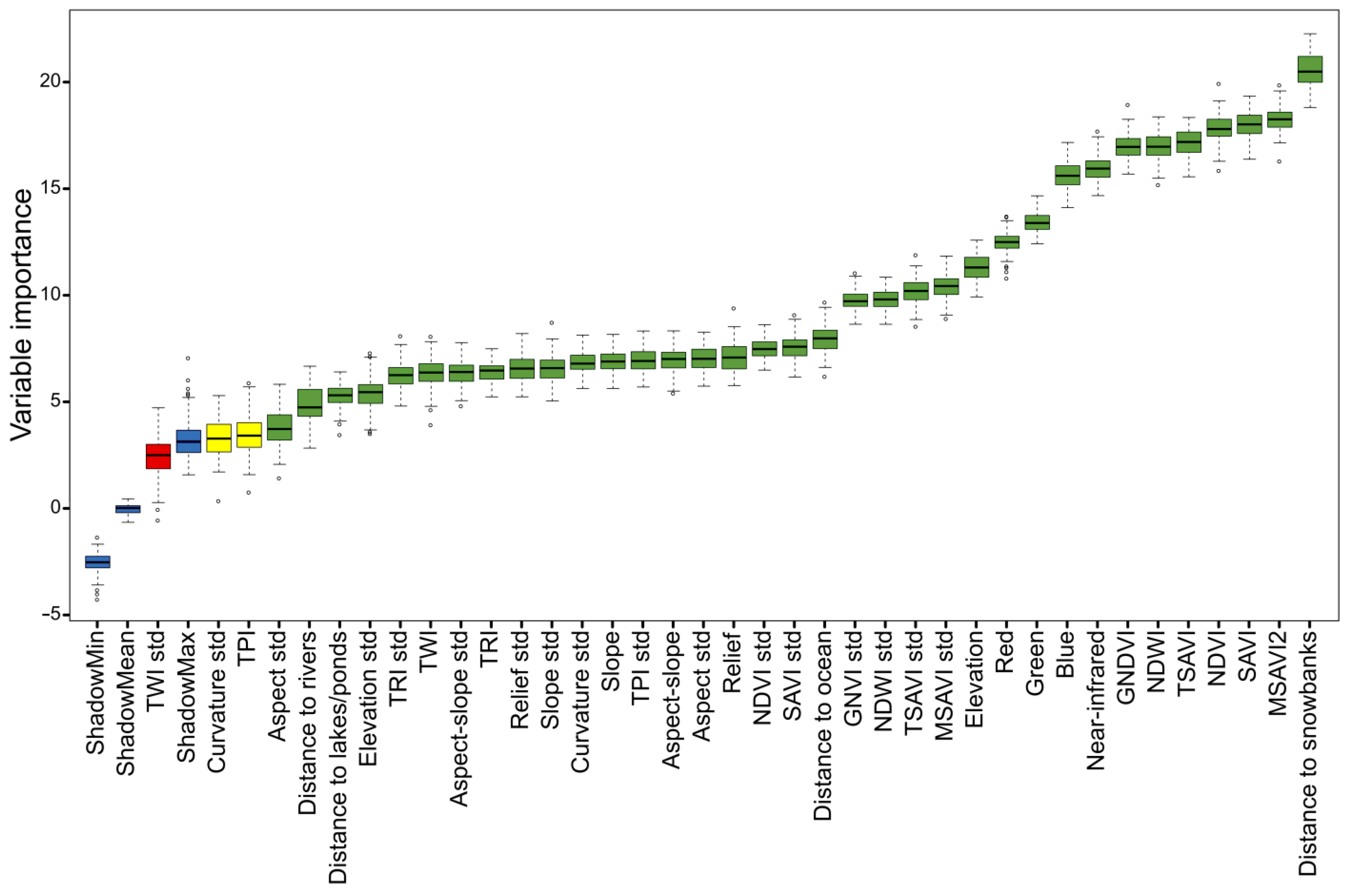
3.1. Assessment of Predictor Importance

Five predictors had AUCs of <0.80 for all seven land cover classes (

Table 3. Area under the receiver operator characteristic curve (AUC) as a measure of predictor relevance for each land cover class. Asterisks indicate AUCs < 0.80 for all seven classes.

Predictor	Forb- Dominated Barren	Forb- Dominated Tundra	Grass- Dominated Wetland	Sedge-Dominated Wetland	Moss- Dominated Wetland	Water	Snow
Spectral predictors
Blue	0.93	0.99	1.00	0.99	0.98	1.00	0.99
Green	0.89	1.00	1.00	1.00	0.97	1.00	0.99
Red	0.85	1.00	0.99	1.00	0.96	0.99	0.98
Near-infrared	0.77	1.00	0.64	1.00	0.87	0.84	0.58
Vegetation predictors
GNDVI	0.94	0.95	1.00	0.95	1.00	1.00	1.00
GNDVI std	0.84	0.99	0.81	0.99	0.91	0.88	0.79
MSAVI2	0.96	0.96	1.00	0.96	1.00	1.00	1.00
MSAVI2 std	0.63	0.98	0.94	0.98	0.63	0.90	0.78
NDVI	0.96	0.96	1.00	0.96	1.00	1.00	1.00
NDVI std	0.71	0.95	0.68	0.95	0.76	0.70	0.58
SAVI	0.96	0.96	1.00	0.96	1.00	1.00	1.00
SAVI std	0.70	0.95	0.68	0.95	0.76	0.70	0.58
TSAVI	0.96	0.96	1.00	0.96	1.00	1.00	0.98
TSAVI std	0.88	0.83	0.98	0.88	0.98	1.00	0.97
Topographic predictors
Aspect *	0.68	0.68	0.76	0.68	0.63	0.65	0.72
Aspect std *	0.64	0.70	0.64	0.70	0.64	0.64	0.64
Aspect–slope	0.71	0.83	0.71	0.83	0.93	0.71	0.74
Aspect–slope std	0.72	0.84	0.72	0.84	0.92	0.72	0.76
Curvature *	0.58	0.65	0.58	0.65	0.60	0.57	0.63
Curvature std	0.73	0.83	0.70	0.83	0.96	0.70	0.73
Elevation	0.70	0.70	0.70	0.69	0.70	0.87	0.70
Elevation std	0.56	0.89	0.74	0.89	0.52	0.81	0.73
Relief	0.73	0.83	0.69	0.83	0.96	0.69	0.72
Relief std	0.72	0.83	0.71	0.83	0.95	0.71	0.74
Slope	0.73	0.83	0.69	0.83	0.96	0.69	0.72
Slope std	0.73	0.83	0.71	0.83	0.95	0.71	0.73
TPI *	0.58	0.66	0.62	0.66	0.58	0.62	0.65
TPI std	0.73	0.83	0.70	0.83	0.96	0.70	0.73
TRI	0.74	0.80	0.68	0.80	0.96	0.68	0.70
TRI std	0.71	0.76	0.71	0.76	0.90	0.62	0.66
Hydrological predictors
Distance to lakes/ponds	0.56	0.84	0.60	0.84	0.61	0.57	0.53
Distance to ocean	0.65	0.64	0.64	0.65	0.64	0.88	0.64
Distance to rivers *	0.62	0.59	0.60	0.62	0.73	0.64	0.61
Distance to snowbanks	1.00	0.58	0.57	1.00	1.00	0.67	0.52
NDWI	0.94	0.95	1.00	0.95	1.00	1.00	1.00
NDWI std	0.84	0.99	0.81	0.99	0.91	0.88	0.79
TWI	0.74	0.83	0.74	0.83	0.95	0.74	0.76
TWI std	0.67	0.68	0.51	0.68	0.73	0.72	0.51

), that is aspect, standard deviation of aspect, curvature, distance to rivers, and the TPI. The most relevant predictors (AUC ≥ 0.99) allowing the discrimination of land cover classes differed among the classes (Table 3). For the forb-dominated barren, distance to the nearest snowbank was the most relevant predictor. It had the largest mean distance from a snowbank (440 m) among the vegetation classes (Table S2). For the forb-dominated tundra, the four spectral bands, as well as the standard deviations of the GNDVI and the NDWI were the most relevant predictors. In the grass-dominated wetland and water classes, the blue, green, and red bands, as well as all the mean values of the vegetation indices and the NDWI were equally relevant. For the sedge-dominated wetland, the top predictors included the four spectral bands, the distance to snowbanks, as well as the standard deviations of the GNDVI and the NDWI. For the moss-dominated wetland, all the mean values of the vegetation indices, the mean NDWI, and the distance to snowbanks were equally relevant. For the snow class, the blue and green bands, the mean NDWI, and all the mean values of the vegetation indices (except the TSAVI) were the most relevant. Surprisingly, distance to the nearest snowbank was not as relevant in discriminating snow (AUC = 0.52), although the mean distance and the standard deviation to a snowbank were 0 (Table S2).

According to the output of Boruta, 35 predictors were considered important, with distance to snowbanks being the most important predictor, followed by the MSAVI2 and the SAVI (Figure 3). One predictor (the standard deviation of the TWI) was considered unimportant. Boruta did not allow the importance of the TPI and the standard deviation of curvature to be concluded.

The correlogram indicated perfect correlation between the relief, the TRI, the standard deviation of TPI, and the standard deviation of curvature (Figure S2). Among these four predictors, we retained relief as it had the highest importance score according to the Boruta analysis (Figure 3). There was also a correlation of 1 between the SAVI and the NDVI and between the NDWI and the GNDVI, whether mean values or standard deviations were used as predictors. We retained the SAVI and the NDWI (mean and standard deviation), as they had higher importance scores according to Boruta (Figure 3).

Overall, our assessment of predictor performance allowed us to exclude 13 predictors from the classification analyses. Aspect, standard deviation of aspect, curvature, distance to rivers, and the TPI were excluded because they were not highly relevant with either one of the land cover classes (i.e., AUCs < 0.80). Standard deviation of the TWI and standard deviation of curvature were excluded because their inclusion did not improve the accuracy of the model according to Boruta results (the TPI was also discarded with Boruta). The NDVI, GNDVI, standard deviation of the NDVI, standard deviation of the GNDVI and the TRI, and standard deviation of the TPI were excluded because they were redundant and collinear based on the correlation matrix (the standard deviation of curvature was discarded again due to its perfect correlation with relief).

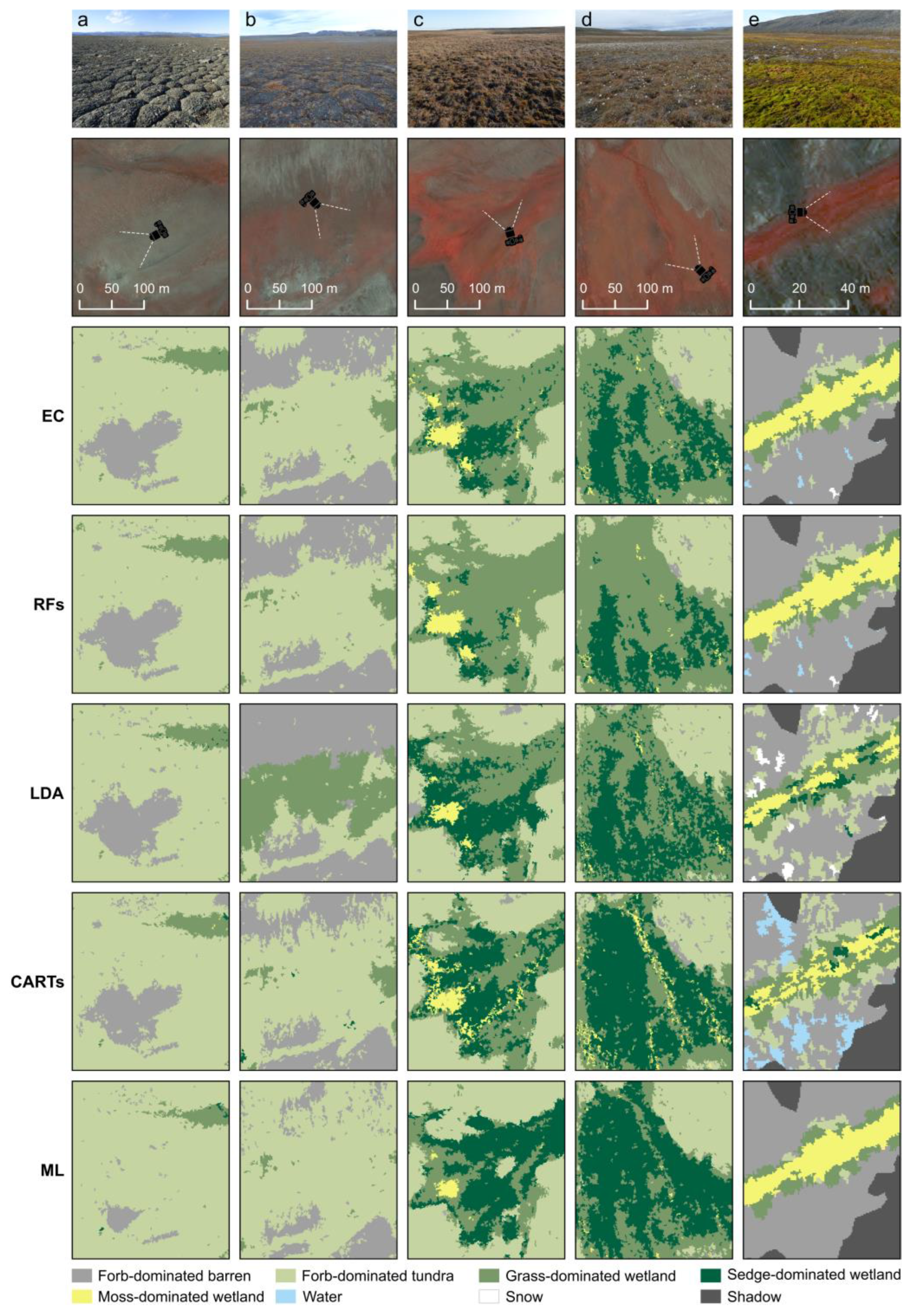
3.2. Image Classification and Validation

The overall accuracies of the classifiers ranged between 75% and 88% (

Table 4. Balanced accuracy (%) of seven land cover classes derived from confusion matrices for nine classifiers. Bottom rows indicate the overall accuracy (%) and Kappa coefficient for each classifier.

Land Cover Class	RFs	ANNs	NB	EC	SVMs	LDA	CARTs	ML	KNNs
Forb-dominated barren	93.0	94.4	88.9	90.9	88.1	85.9	93.4	86.8	82.5
Forb-dominated tundra	83.4	88.7	86.8	82.1	84.1	83.4	83.7	87.5	76.1
Grass-dominated wetland	89.1	89.8	82.7	81.5	86.6	89.8	70.2	74.4	70.5
Sedge-dominated wetland	83.3	74.4	90.0	82.8	81.6	82.2	80.1	73.3	79.3
Moss-dominated wetland	100.0	99.4	99.4	100.0	99.4	100.0	99.4	100.0	89.4
Water	100.0	99.4	100.0	100.0	99.4	96.2	100.0	100.0	100.0
Snow	100.0	96.9	100.0	100.0	100.0	93.8	100.0	100.0	99.3
Overall accuracy (95% confidence interval)	88.0 (79.6–93.9)	88.0 (79.6–93.9)	85.9 (77.1–92.3)	84.8 (75.8–91.4)	84.8 (75.8–91.4)	82.6 (73.3–89.7)	81.9 (72.0–89.5)	81.5 (72.1–88.9)	75.0 (64.9–83.5)
Kappa coefficient	85.6	85.6	83.1	81.7	81.8	79.0	78.5	77.8	70.1

RFs (random forests), ANNs (artificial neural networks), NB (naive Bayes), EC (ensemble classifier), SVMs (support vector machines), LDA (linear discriminant analysis), CARTs (classification and regression trees), ML (maximum likelihood), KNNs (K-nearest neighbors).

). There was strong overlap between the confidence intervals of the overall accuracy of the classifiers, thus they were not considered statistically different. However, upon close visual inspection and cross-checking of the classifier results with known land classes in the field, some discrepancies were discernible. Notably, all classifiers wrongly classified, as water or grass-dominated wetland, the unmasked shadow that was produced by boulders at a resolution <2 m, which is the resolution of the ArcticDEM hillshade (Figure S3). Some snowbanks covered by soil material (e.g., till and gravel) had darker surfaces and were classified as forb-dominated barren instead of snow (Figure S4). In addition, the ANN, SVM, NB, and KNN classifiers consistently classified rocky areas on the illuminated side of canyons as snow instead of forb-dominated barren (Figure 4). Due to this extended misclassification, these four classifiers were not included in the EC.

Regardless of which classifiers were used, all land cover classes had a balanced accuracy of >0.70 and were thus relatively well discriminated (Table 4). Moss-dominated wetland, water, and snow were the best discriminated classes due to their balanced accuracy of >0.89 for all classifiers.

Combining multiple classifiers by taking the prediction majority in the EC reduced the bias appearing in some individual classifiers. In some cases, the CARTs, LDA, RFs and ML misclassified the vegetation, but by taking the majority, the EC was less influenced by these errors. For example, in Figure 5 (column a), ML was unable to detect the patch of forb-dominated barren, while RFs, LDA, and CARTs did so successfully, which translated into the EC correctly predicting that patch. Similarly, LDA is the only classifier to have misclassified a patch of forb-dominated tundra as grass-dominated wetland (Figure 5, column b). In Figure 5 (column e), the RFs and ML correctly classified the patch as moss-dominated wetland, while the LDA and CARTs partially detected it, hence the EC prediction was accurate. On the other hand, in the few cases where two or more classifiers generated classification errors, these errors also appeared in the EC classification. For example, in Figure 5 (column c), RFs were the only classifier correctly classifying the patch as grass-dominated wetland, while the other classifiers predicted a larger area of sedge-dominated wetland. As a result, this error also appeared in the EC. Based on our field observations, the patch in Figure 5 (column d) should have been classified almost entirely as sedge-dominated wetland in the EC, but this was not the case as only the CARTs and ML correctly predicted this vegetation class.

3.3. Final Land Cover Map

We calculated a confusion matrix based on the classification resulting from the EC. The confusion matrix showed that moss-dominated wetland, water, and snow were accurately classified, with both producer’s and user’s accuracies reaching 100% (

Table 5. Confusion matrix derived from independent validation dataset and classification predictions of an ensemble classifier, based on four algorithms, namely random forests, linear discriminant analysis, classification and regression trees, and maximum likelihood.

	Reference (Actual Classes)
		Forb- Dominated Barren	Forb- Dominated Tundra	Grass- Dominated Wetland	Sedge-Dominated Wetland	Moss- Dominated Wetland	Water	Snow	Total	User’s Accuracy (%)
Prediction (predicted classes)	Forb-dominated barren	20	1	0	0	0	0	0	21	95.2
	Forb-dominated tundra	4	11	3	0	0	0	0	18	61.1
	Grass-dominated wetland	0	3	9	2	0	0	0	14	64.3
	Sedge-dominated wetland	0	0	1	4	0	0	0	5	80.0
	Moss-dominated wetland	0	0	0	0	5	0	0	5	100.0
	Water	0	0	0	0	0	13	0	13	100.0
	Snow	0	0	0	0	0	0	16	16	100.0
	Total	24	15	13	6	5	13	16	92
	Producer’s accuracy (%)	83.3	73.3	69.2	66.7	100.0	100.0	100.0		84.8

). The main confusion was for the sedge-dominated wetland (omission error = 33%), which was confused with the grass-dominated wetland (Table 5). The commission error was relatively high (36–39%) for the forb-dominated tundra and the grass-dominated wetland (Table 5). Some validation points classified as forb-dominated tundra actually belonged to forb-dominated barren and grass-dominated wetland, while some points classified as grass-dominated wetland belonged, in reality, to forb-dominated tundra and sedge-dominated wetland (Table 5). The confusion matrix, which is based on validation points representing 20% of all reference data, led to a very small validation sample size for sedge-dominated wetland and moss-dominated wetland (Table 2). This makes the accuracy metrics more difficult to interpret for these land cover classes, as there were relatively few opportunities to test accuracy in these classes.

Over the entire land area of 162 km² (including lakes) (Figure 6), the forb-dominated tundra had the largest areal coverage (44.9%), followed by forb-dominated barren (33.9%), grass-dominated wetland (12.8%), shadow (2.9%), water (2.4%), human infrastructure (1.1%), sedge-dominated wetland (1.0%), snow (0.5%), and moss-dominated wetland (0.5%).

4. Discussion

The Arctic is changing rapidly, and remote sensing is increasingly used to understand the causes and consequences of these changes. For example, land cover mapping provides a tool for the comparable and repeated monitoring of changes over time. Due to the high spatial heterogeneity of vegetation and terrain in the Arctic, there is no universal methodology to classify all Arctic terrestrial ecosystems with high accuracy. However, ecosystem mapping would benefit from the contributions of local ecosystem classifications sharing lessons learned and best practices. Hence, several studies spread across the circumpolar world have tested and proposed methods that were most relevant to their site and objectives. Here, we presented a methodology to produce a very accurate land cover map of the surroundings of the Canadian Forces Station Alert on Ellesmere Island (Nunavut, Canada). Our methodological scheme is based on a combination of existing or commonly used procedures, algorithms, and predictors but differs from other studies published in the Arctic by including water-related predictors and combining multiple classifiers in an ensemble. Our study is also among the few taking place in a polar desert, a landscape that is both the most representative and least studied of the High Arctic. In the following sections, we assess the predictor importance and discuss the classification performance of popular classifiers compared to the EC. Finally, we compile recommendations to improve the development of land cover maps in High Arctic regions, which should significantly advance the monitoring of Arctic ecosystems.

4.1. Predictor Importance

Among the 25 predictors used for classification, distance to snowbanks, the MSAVI2, the SAVI, the TSAVI, and the NDWI were the top five predictors allowing the discrimination of land cover classes in our study area (Figure 3). Although the NDVI was among the most important predictors, it was discarded from the classification due to its perfect correlation with the SAVI (Figure S2). It should be mentioned that the importance scores of these vegetation indices were only slightly higher than the nonsoil-adjusted vegetation indices, the NDVI, and the GNDVI. As in other studies [6,122], topographic predictors were less important, which is surprising as topography drives soil moisture and water flow.

Predictor importance may suggest underlying biophysical mechanisms [6]. For example, the NDWI and distance to the nearest snowbank increased classification accuracy and thus highlight that water availability is crucial to predict vegetation classes in polar deserts. The water table depth and soil moisture are intrinsically linked to vegetation cover and diversity in Arctic ecosystems [65,123,124]. Although the NDWI was designed for the extraction and mapping of water area boundaries [95], it also appears to be sensitive to changes in soil water content. Indeed, the NDWI was among the most relevant predictors (AUC = 1.00) for discriminating the water class (represented by small ponds and rivers) and two wetlands (represented by grass-dominated wetland and moss-dominated wetland) (Table 3).

Water in the form of snow is one of the most important determinants of ecosystem functions in high-latitude and high-altitude regions, where snow dominates the landscape for most of the year [125,126,127,128,129]. During summer, perennial snowbanks gradually melt, generating an inflow of melt water to areas downslope, thus influencing the richness, composition, and biomass of plant communities [127,130,131,132,133]. Snow cover also increases soil temperatures, which, in turn, increases nutrient availability via decomposition [134,135]. Uneven snow accumulation produces a wide spectrum of habitats, therefore enabling the regional co-occurrence of a large range of species with contrasted ecological requirements, from chionophilous (snow-dependent) to chionophobous (snow-avoiding) species [136]. For example, the forb-dominated barren, the driest vegetation class, had the furthest mean distance from a snowbank (Table S2). In addition, we found that distance to snowbanks emerged as the most important predictor of sedge-dominated wetland, thus confirming Desjardins et al. [75], who had demonstrated at the same site an association between this community and perennial snowbanks. To our knowledge, snowbanks were never previously used as a predictor of vegetation classification in the Arctic. Nonetheless, some studies included snow as a predictor in species distribution models or community models. Specifically, incorporating remotely sensed snow persistency in species distribution models helps predict the distribution of several vascular plants, mosses, and lichens in northern Norway [137]. Another study modeled the distribution of one Arctic dwarf shrub species in Svalbard using the snow cover derived from one satellite imagery taken in summer [138]. We recommend not neglecting information on snow in the vegetation classifications of Arctic ecosystems where topographic heterogeneity generates uneven snow accumulation and duration. The quantity, quality, and seasonality of snow are projected to change all over the tundra biome, although to varying extents depending on the region [125,126,133]. This will lead to changes in the distribution and composition of Arctic plant communities, with cascading effects on many ecological processes [125], further justifying the monitoring of snowbank shrinkage through repeated ecosystem classifications over time.

Soil-adjusted vegetation indices, developed to counteract the sensitivity of the NDVI to soil background in hot deserts, can also be useful for polar deserts. Like hot deserts, polar deserts have large expanses of bare soil [53]. Although soil-adjusted indices were effective in classifying land cover classes in this study, another study conducted in Alaska indicated that the NDVI was more strongly correlated to plant biomass than the soil-adjusted indices [139]. However, vegetation cover was significantly more extensive in the Alaska study area than at our site, which may explain why the SAVI was not as effective at detecting canopy variables in their case. In a northern grassland in Saskatchewan, the TSAVI was more correlated with biophysical parameters (e.g., leaf area index, percentage of bare ground, and canopy height) than the NDVI [140]. The algorithm of the TSAVI takes into account the slope and intercept of the soil line, which must be calculated specifically for the site under study; these additional computations significantly limit its application [141]. In our study, soil-adjusted indices performed only slightly better than regular, nonsoil-adjusted vegetation indices. Considering that each vegetation index has its limitations and specificities, we advise testing several of them and identifying those most suitable for the study site.

4.2. Classification Performance

Except for KNNs, all classifiers had a high overall accuracy (>81%; Table 4). The RF classifier yielded a high accuracy, as confirmed by all accuracy scores and the visual assessment of the classified map (Table 4, Figure 4 and Figure 5), which justifies its popular use in other Arctic ecosystem classifications (e.g., [1,7,38,39,40]). Surprisingly, a study in the polar desert of Melville Island (Nunavut) comparing ML, RFs and SVMs found that SVMs produced the highest classification accuracy (overall classification accuracy = 90.7%) for eight land cover classes [44]. These contrasting results suggest that the selection of classifiers is important to improve vegetation mapping in a given environment because no image classifier is superior for all applications [4].

There were some noticeable discrepancies in the predictions of the ANNs, SVMs, NB, and KNNs where the illuminated side of canyons were classified as snow instead of forb-dominated barren (Figure 4). In addition, because the ArcticDEM from which the hillshade originated had a coarser resolution (2 m) than the satellite imagery (0.5 m), several small, shadowed areas were not masked prior to the classification. As a result, these shadowed areas were mostly classified as water (Figure S3). The extent of these misclassifications represented <1% of the study area, thus not compromising the use of the final map for identifying wildlife habitats and selecting monitoring sites. The confusion between shadowed areas and water is recurrent in classification studies performed at high resolution [7,48,142], as water shares similar spectral characteristics as shadows [142]. Even creating an additional class for shadow in the classification (instead of creating a shadow layer using a hillshade) did not solve the problem as there were several water areas classified as shadow and vice versa (results not shown). Higher resolution DEMs should be available for Arctic regions in the next few years, which will allow the computation of more accurate hillshades and solve this issue. Another misclassification included a few snowbanks that were classified as forb-dominated barren when they were covered by till and gravel (Figure S4). This could explain why the distance to snowbanks was not among the most important predictors to discriminate snow (Table 3). It was previously observed that fresh snow had very high reflectivity in the visible and near-infrared, but its reflectivity decreased over time as dirt accumulated and darkened the surface, inducing classification errors [59].

Combining multiple classifiers should increase the overall classification accuracy or at least achieve an overall accuracy equivalent to the best performing algorithms [66,143,144]. We found that the EC had a high accuracy (84.8%) comparable to that of RFs (88%, confidence intervals overlapping; Table 4). Nevertheless, a visual comparison of satellite imagery and classified maps suggested that using the EC allowed a better delineation of land cover patches than using RFs. The EC has other advantages, such as reducing classification bias appearing in individual classifiers (Figure 5a,b,e). However, where ≥2 (out of 4) classifiers misclassified land cover classes, these errors were repeated into the final classification of the EC (Figure 5c,d). One solution to further reduce errors would be to combine more classifiers, as the higher the number of classifiers, the more diluted the classification errors are [66]. Considering no individual classifier is perfect, combining the most accurate ones represents a good compromise and may overcome difficulties in selecting one specific classifier. We thus retained the map classified using the EC for future uses at Alert.

According to the confusion matrix of the EC, snow, water, and moss-dominated wetland were perfectly discriminated (Table 5), mostly due to their unique spectral signal and their spatial homogeneity [38]. More confusion, however, occurred between the remaining vegetation classes. The verification of misclassified points indicated that errors occurred mostly due to transitional states between communities, such as when forb-dominated barren was confused with forb-dominated tundra, or forb-dominated tundra was confused with grass-dominated wetland. Such confusions can be explained because the above pairs are composed of the same plant species but with an ascending percentage of coverage. Similarly, errors occurred due to a retrogression from one community to another (e.g., from grass-dominated wetland to forb-dominated tundra, the latter characterized by a high number of dead stems of Alopecurus magellanicus Lamarck) or due to the presence of mixed communities (e.g., grass-dominated and sedge-dominated wetlands were sometimes intermingled within the same lush patches of vegetation) [75]. Some misclassifications between the vegetation classes could also be related to soil humidity. The level of soil moisture underlying vegetation can modify the spectral reflectance captured by the satellite [45,145,146]. For example, moist areas produce higher NDVI values than dry or wet environments [147]. Furthermore, grass- and sedge-dominated wetlands being both dominated by graminoids characterized by vertically oriented, linear-shape foliage, their spectral signature may not be sufficiently different to separate them efficiently when not in flower. The linear foliage of graminoids may present a challenge for top-down remote sensing because most of the leaf area is not apparent to the sensor [59]. Overall, this reflects the difficulty in classifying perfectly plant communities in the High Arctic, which are often characterized by low species diversity, large overlap in species composition, and gradual rather than abrupt differences in vegetation cover [122].

4.3. Challenges and Recommendations

Our case study and literature review highlight a few challenges and generate several recommendations regarding the adequate mapping of land cover classes in polar deserts and other High Arctic regions. We structure these challenges and recommendations according to nine themes that are common to most land cover mapping exercises.

4.3.1. Spectral Resolution

The literature suggests that classification performance increases with spectral resolution [44,148]. The inclusion of extra spectral data, whether in single bands or vegetation indices, may reveal distinct characteristics of biotic and abiotic covers invisible to wider spectral bands of multispectral imagery, including plant vigor and senescence, soil saturation, litter materials, or background rock [1,4]. For example, due to their ability to detect the strong absorption of cellulose and lignin, short-wave infrared (SWIR) bands (not available in the Worldview imagery used in this study) are useful to study High Arctic vegetation, where there is a higher proportion of senescent or dry vegetation than in the Low Arctic [145,146].

4.3.2. Spatial Resolution

The ideal scale for mapping vegetation and other land cover classes depends largely on the purposes of the map. Medium spatial resolution (20–30 m) is widely used to define terrestrial mammal habitats [5]. High spatial resolution (<5 m) is typically required for monitoring plant community changes over time in heterogeneous Arctic landscapes [1,147,149]. However, if species-level or functional type-level maps are needed, even higher spatial resolution (<2 m) may be required [45,59].

4.3.3. Image Acquisition Date

The ability of satellite images to capture spatial variation in vegetation depends on plant phenology at the time of image acquisition [50,150]. Capturing the peak growth of all plant groups (e.g., shrubs, forbs, graminoids, mosses, and lichens) in a single satellite image is not possible [150]. To address this challenge, spectral bands taken at different times during the growing season can be used as predictors [6,50]. When it is impossible to acquire several pictures due to high costs or cloud cover limitations, knowledge of the phenology of the study site is important to adequately choose the date of the satellite imagery. For example, we chose a date in 2020 when graminoids had reached their peak growth that year as they are indicator species for two wetland communities at Alert [75].

4.3.4. Image Segmentation

Image segmentation depends on the spatial resolution of the initial imagery. When using high resolution datasets, object-based methods are usually preferred over pixel-based methods [98]. Reasons for this choice include (1) vegetation patches are usually larger than pixels, hence pixels can be merged into homogeneous segments; (2) several land cover types have a large internal heterogeneity in very high-resolution images, often due to shadow effects caused by higher vegetation and boulders, which hamper pixel-based classifications; and (3) generated homogeneous segments are a more realistic construction of the landscape elements than pixels, and they better mimic human (and wildlife) interpretation of the landscape [151].

When the segmentation method and its parameterization are chosen carefully, they lead to improved classifications compared to pixel-based methods [42,152]. One of the most important parameters is the segment size, which depends on the resolution requirements. The optimal size of a segment is the largest size providing an adequate delineating of the different land cover classes [38]. For example, there was a lower (2.5 m²) and an upper (5 m²) limit for the optimal segmentation size to produce the most accurate classification for a mosaicked peatland in Northern Finland [1]. The optimal segmentation size for classification depends on the patchiness of vegetation and land cover types in the study area and should be tested for every studied landscape. In addition, layers used to generate the segmentation can be important. In our study, we used multispectral bands as they were sufficient to differentiate land cover classes, but it is possible to add other types of layers. For example, A’Campo et al. [38] based their segmentation upon the near-infrared band, the green band, the NDVI, and some DEM-derived layers.

4.3.5. Land Cover Classes

The optimal number of land cover classes and the definition of each land cover class depend on the purposes of the map. For wildlife habitat mapping, four to eight classes are generally recommended [5]. There is no standard nomenclature for categorizing local-scale land cover classes in the Arctic [6]. Nevertheless, using functional types is increasingly put forward [40,50,153,154]. Broad physiognomic vegetation maps have limitations for long-term monitoring because temporal changes in vegetation properties more likely involve shifts in species composition than transitions across broad vegetation classes [6]. Chapin et al. [155] thus recommended using Arctic-specific plant functional types in classifications aimed at capturing vegetation change through time. The suggested functional types included deciduous shrubs, evergreen shrubs, sedges, grasses, forbs, Sphagnum L. moss, non-Sphagnum moss, and lichens.

To obtain good classification accuracy, land cover classes must have good spectral separability, which often implies a limited number of classes [44]. Increasing the number of classes can reduce accuracy, which was the case when we initially attempted to divide the forb-dominated barren into bare ground (5% mean plant cover) and xeric area (20% mean plant cover).

4.3.6. Ground Truth Points

Land cover maps are only as credible as the underlying training data [59]. A sufficiently large and representative training dataset helps prevent misclassification. Ground reference points usually range between 9 and 112 per class [24,39,44], whereas we used 25–120 reference points per class (Table 2). To increase the accuracy of our maps, it was necessary for the reference points to cover the full extent of spectral heterogeneity within each land cover class, hence the addition of points through photo interpretation in our methodology. Field data, however, provide a more reliable validation reference than photo-interpreted data [59].

4.3.7. Predictors and Predictor Selection

Multiple predictors achieved a higher accuracy than more parsimonious models, which is consistent with the literature [1,7,122]. For example, when using the top five predictors (distance to snowbanks, the MSAVI2, the SAVI, the TSAVI, and the NDWI), we obtained lower overall accuracies (RFs: 78.3%, ANNs: 80.4%, NB: 69.6%, SVMs: 71.7%, LDA: 70.7%, CARTs: 79.4%, ML: 80.4%, and KNNs: 73.9%) than when using the 25 selected predictors (Table 4). However, selecting predictors is important as it eliminates unimportant predictors and improves the performance of the classification [100]. Except for KNNs and LDA, the overall accuracy of the individual classifiers was lower, especially for ML, when using all 38 predictors (RFs: 84.8%, ANNs: 80.4%, NB: 80.4%, SVMs: 82.6%, LDA: 82.6%, CARTs: 79.4%, ML: 61.4%, KNNs: 81.5%).

Predictor selection requires an understanding of the studied ecosystem to filter suitable predictors [7]. In our case study, we knew that perennial snowbanks were sustaining the sedge-dominated wetlands, thus we included distance to the nearest snowbank as a potential predictor. We recommend including distance to the nearest snowbank or other snow-related predictors (e.g., the day of snow disappearance for each pixel) in future classifications, especially in Arctic environments with heterogeneous topography. Furthermore, given that each vegetation index has its limitations and specificities, we advise testing several of them and identifying those most suitable to the study site.

4.3.8. Classification Algorithms

There is no superior classification method that can be applied universally [4], therefore searching improved classifiers is important for remote sensing applications. We recommend testing several classifiers and selecting the one that fits best. Alternatively, several classifiers can be used to generate an ensemble model. We implemented and tested in R a multiclass ensemble classifier based on majority voting, which performed well. There are other ways of combining classifiers (e.g., weighted voting, stacking, boosting, and bagging) [66] that are worth exploring.

4.3.9. Classification Validation

While some studies evaluate the final map visually to assess classification performance [1,7], others only rely on accuracy metrics [44,48]. We consider visual evaluation of the final classified map as a critical addition to accuracy metrics. Indeed, although it requires time and knowledge of the area and involves subjectivity [4], accuracy metrics are not infallible. We found that the best performing classifiers did not all have the highest overall accuracies, and, conversely, some classifiers with multiple erroneous predictions had among the highest overall accuracies.

5. Conclusions

The last two decades have seen significant improvements in the ability to produce land cover maps of Arctic ecosystems through remote sensing. However, due to the fine-scale spatial heterogeneity of Arctic ecosystems, the main challenge remains to bridge the information extracted from satellite imagery with the cover classes identified on the ground. Moreover, as each region has its own specificities in terms of land cover classes, vegetation structure, topography, and soil composition, there is no universal and transferable method for all Arctic sites. Therefore, several studies spread across the circumpolar Arctic have tested and proposed methods that were most relevant for their study site and needs. Here, we found that some water-related indices and soil-adjusted indices were the most effective predictors for discriminating land cover classes in a polar desert. In addition, the ensemble classifier based on a majority voting algorithm yielded satisfactory predictions. Using an ensemble classifier also avoided the need to choose a specific classifier. These results can assist researchers in generating land cover classifications in the High Arctic serving their own applications. We also argue that more detailed case studies, such as ours, are needed to reflect the full variability of approaches pertinent to mapping land cover in the Arctic. Arctic ecosystems are changing fast, and remote sensing techniques no doubt offer some of the most useful tools for detecting and monitoring ongoing and future changes.

References

1. Räsänen, A.; Virtanen, T. Data and resolution requirements in mapping vegetation in spatially heterogeneous landscapes. Remote Sens. Environ. 2019, 230, 111207. [Google Scholar] [CrossRef]
2. Kamusoko, C. Remote Sensing Image Classification in R; Springer Nature: Singapore, 2019; p. 189. [Google Scholar]
3. Borra, S.; Thanki, R.; Dey, N. Satellite Image Analysis: Clustering and Classification; Springer Nature: Singapore, 2019; p. 97. [Google Scholar]
4. Xie, Y.; Sha, Z.; Yu, M. Remote sensing imagery in vegetation mapping: A review. J. Plant Ecol. 2008, 1, 9–23. [Google Scholar] [CrossRef]
5. Bartsch, A.; Höfler, A.; Kroisleitner, C.; Trofaier, A.M. Land Cover Mapping in Northern High Latitude Permafrost Regions with Satellite Data: Achievements and Remaining Challenges. Remote Sens. 2016, 8, 979. [Google Scholar] [CrossRef] [Green Version]
6. Macander, M.J.; Frost, G.V.; Nelson, P.R.; Swingley, C.S. Regional Quantitative Cover Mapping of Tundra Plant Functional Types in Arctic Alaska. Remote Sens. 2017, 9, 1024. [Google Scholar] [CrossRef] [Green Version]
7. Eischeid, I.; Soininen, E.M.; Assmann, J.J.; Ims, R.A.; Madsen, J.; Pedersen, A.Ø.; Pirotti, F.; Yoccoz, N.G.; Ravolainen, V.T. Disturbance Mapping in Arctic Tundra Improved by a Planning Workflow for Drone Studies: Advancing Tools for Future Ecosystem Monitoring. Remote Sens. 2021, 13, 4466. [Google Scholar] [CrossRef]
8. Post, E.; Forchhammer, M.C.; Bret-Harte, M.S.; Callaghan, T.V.; Christensen, T.R.; Elberling, B.; Fox, A.D.; Gilg, O.; Hik, D.S.; Høye, T.T.; et al. Ecological Dynamics Across the Arctic Associated with Recent Climate Change. Science 2009, 325, 1355–1358. [Google Scholar] [CrossRef] [Green Version]
9. Rantanen, M.; Karpechko, A.Y.; Lipponen, A.; Nordling, K.; Hyvärinen, O.; Ruosteenoja, K.; Vihma, T.; Laaksonen, A. The Arctic has warmed nearly four times faster than the globe since 1979. Commun. Earth Environ. 2022, 3, 168. [Google Scholar] [CrossRef]
10. Wookey, P.A.; Aerts, R.; Bardgett, R.D.; Baptist, F.; Bråthen, K.A.; Cornelissen, J.H.C.; Gough, L.; Hartley, I.P.; Hopkins, D.W.; Lavorel, S.; et al. Ecosystem feedbacks and cascade processes: Understanding their role in the responses of Arctic and alpine ecosystems to environmental change. Glob. Chang. Biol. 2009, 15, 1153–1172. [Google Scholar] [CrossRef] [Green Version]
11. Chapin, F.S., III; Sturm, M.; Serreze, M.C.; McFadden, J.P.; Key, J.R.; Lloyd, A.H.; McGuire, A.D.; Rupp, T.S.; Lynch, A.H.; Schimel, J.P.; et al. Role of Land-Surface Changes in Arctic Summer Warming. Science 2005, 310, 657–660. [Google Scholar] [CrossRef]
12. Elmendorf, S.C.; Henry, G.H.R.; Hollister, R.D.; Björk, R.G.; Bjorkman, A.D.; Callaghan, T.V.; Collier, L.S.; Cooper, E.J.; Cornelissen, J.H.C.; Day, T.A.; et al. Global assessment of experimental climate warming on tundra vegetation: Heterogeneity over space and time. Ecol. Lett. 2012, 15, 164–175. [Google Scholar] [CrossRef]
13. Hansen, B.B.; Grøtan, V.; Aanes, R.; Sæther, B.-E.; Stien, A.; Fuglei, E.; Ims, R.A.; Yoccoz, N.G.; Pedersen, A.Ø. Climate Events Synchronize the Dynamics of a Resident Vertebrate Community in the High Arctic. Science 2013, 339, 313–315. [Google Scholar] [CrossRef] [Green Version]
14. Kerbes, R.H.; Kotanen, P.M.; Jefferies, R.L. Destruction of Wetland Habitats by Lesser Snow Geese: A Keystone Species on the West Coast of Hudson Bay. J. Appl. Ecol. 1990, 27, 242–258. [Google Scholar] [CrossRef]
15. Beamish, A.; Raynolds, M.K.; Epstein, H.; Frost, G.V.; Macander, M.J.; Bergstedt, H.; Bartsch, A.; Kruse, S.; Miles, V.; Tanis, C.M.; et al. Recent trends and remaining challenges for optical remote sensing of Arctic tundra vegetation: A review and outlook. Remote Sens. Environ. 2020, 246, 111872. [Google Scholar] [CrossRef]
16. Rudy, A.C.; Lamoureux, S.F.; Treitz, P.; Collingwood, A. Identifying permafrost slope disturbance using multi-temporal optical satellite images and change detection techniques. Cold Reg. Sci. Technol. 2013, 88, 37–49. [Google Scholar] [CrossRef]
17. Duguay, C.R.; Zhang, T.; Leverington, D.W.; Romanovsky, V.E. Satellite Remote Sensing of Permafrost and Seasonally Frozen Ground. Remote Sens. North.Hydrol. Meas. Environ. Chang. 2005, 163, 91–118. [Google Scholar] [CrossRef] [Green Version]
18. Hugelius, G.; Routh, J.; Kuhry, P.; Crill, P. Mapping the degree of decomposition and thaw remobilization potential of soil organic matter in discontinuous permafrost terrain. J. Geophys. Res. Biogeosci. 2012, 117, G02030. [Google Scholar] [CrossRef] [Green Version]
19. Boelman, N.T.; Rocha, A.V.; Shaver, G.R. Understanding burn severity sensing in Arctic tundra: Exploring vegetation indices, suboptimal assessment timing and the impact of increasing pixel size. Int. J. Remote Sens. 2011, 32, 7033–7056. [Google Scholar] [CrossRef]
20. Frost, G.V.; Loehman, A.R.; Saperstein, L.B.; Macander, M.J.; Nelson, P.R.; Paradis, D.P.; Natali, S.M. Multi-decadal patterns of vegetation succession after tundra fire on the Yukon-Kuskokwim Delta, Alaska. Environ. Res. Lett. 2020, 15, 025003. [Google Scholar] [CrossRef]
21. Rees, W.G.; Williams, M.; Vitebsky, P. Mapping land cover change in a reindeer herding area of the Russian Arctic using Landsat TM and ETM+ imagery and indigenous knowledge. Remote Sens. Environ. 2003, 85, 441–452. [Google Scholar] [CrossRef]
22. Tømmervik, H.; Johansen, B.; Tombre, I.; Thannheiser, D.; Høgda, K.A.; Gaare, E.; Wielgolaski, F.E. Vegetation Changes in the Nordic Mountain Birch Forest: The Influence of Grazing and Climate Change. Arct. Antarct. Alp. Res. 2004, 36, 323–332. [Google Scholar] [CrossRef]
23. Daniëls, F.J.A.; De Molenaar, J.G. Flora and Vegetation of Tasiilaq, Formerly Angmagssalik, Southeast Greenland: A Comparison of Data Between Around 1900 and 2007. AMBIO 2011, 40, 650–659. [Google Scholar] [CrossRef] [Green Version]
24. Greaves, H.E.; Eitel, J.U.H.; Vierling, A.L.; Boelman, N.T.; Griffin, K.L.; Magney, T.S.; Prager, C.M. 20 cm resolution mapping of tundra vegetation communities provides an ecological baseline for important research areas in a changing Arctic environment. Environ. Res. Commun. 2019, 1, 105004. [Google Scholar] [CrossRef] [Green Version]
25. Prach, K.; Košnar, J.; Klimešová, J.; Hais, M. High Arctic vegetation after 70 years: A repeated analysis from Svalbard. Polar Biol. 2009, 33, 635–639. [Google Scholar] [CrossRef]
26. Provencher-Nolet, L.; Bernier, M.; Levesque, E. Short term change detection in tundra vegetation near Umiujaq, subarctic Quebec, Canada. In Proceedings of the 2014 IEEE Geoscience and Remote Sensing Symposium, Quebec City, QC, Canada, 13–18 July 2014; pp. 4668–4670. [Google Scholar] [CrossRef] [Green Version]
27. Davis, E.L.; Trant, A.J.; Way, R.G.; Hermanutz, L.; Whitaker, D. Rapid Ecosystem Change at the Southern Limit of the Canadian Arctic, Torngat Mountains National Park. Remote Sens. 2021, 13, 2085. [Google Scholar] [CrossRef]
28. Lin, D.H.; Johnson, D.R.; Andresen, C.; Tweedie, C.E. High spatial resolution decade-time scale land cover change at multiple locations in the Beringian Arctic (1948–2000s). Environ. Res. Lett. 2012, 7, 025502. [Google Scholar] [CrossRef] [Green Version]
29. Radosavljevic, B.; Lantuit, H.; Pollard, W.; Overduin, P.; Couture, N.; Sachs, T.; Helm, V.; Fritz, M. Erosion and Flooding—Threats to Coastal Infrastructure in the Arctic: A Case Study from Herschel Island, Yukon Territory, Canada. Estuar. Coasts 2015, 39, 900–915. [Google Scholar] [CrossRef] [Green Version]
30. Danks, F.S.; Klein, D.R. Using GIS to predict potential wildlife habitat: A case study of muskoxen in northern Alaska. Int. J. Remote Sens. 2020, 23, 4611–4632. [Google Scholar] [CrossRef]
31. Pearce, C.M. Mapping Muskox Habitat in the Canadian High Arctic with SPOT Satellite Data. Arctic 1991, 44, 49–57. [Google Scholar] [CrossRef] [Green Version]
32. Edenius, L.; Vencatasawmy, C.P.; Sandström, P.; Dahlberg, U. Combining Satellite Imagery and Ancillary Data to Map Snowbed Vegetation Important to Reindeer Rangifer tarandus. Arct. Antarct. Alp. Res. 2003, 35, 150–157. [Google Scholar] [CrossRef]
33. Fraser, R.; McLennan, D.; Ponomarenko, S.; Olthof, I. Image-based predictive ecosystem mapping in Canadian arctic parks. Int. J. Appl. Earth Obs. Geoinform. 2012, 14, 129–138. [Google Scholar] [CrossRef]
34. Bartsch, A.; Pointner, G.; Ingeman-Nielsen, T.; Lu, W. Towards Circumpolar Mapping of Arctic Settlements and Infrastructure Based on Sentinel-1 and Sentinel-2. Remote Sens. 2020, 12, 2368. [Google Scholar] [CrossRef]
35. Atkinson, D.M.; Treitz, P. Arctic Ecological Classifications Derived from Vegetation Community and Satellite Spectral Data. Remote Sens. 2012, 4, 3948–3971. [Google Scholar] [CrossRef] [Green Version]
36. Elberling, B.; Tamstorf, M.P.; Michelsen, A.; Arndal, M.F.; Sigsgaard, C.; Illeris, L.; Bay, C.; Hansen, B.U.; Christensen, T.R.; Hansen, E.S.; et al. Soil and Plant Community-Characteristics and Dynamics at Zackenberg. Adv. Ecol. Res. 2008, 40, 223–248. [Google Scholar] [CrossRef]
37. Stow, D.A.; Hope, A.; McGuire, D.; Verbyla, D.; Gamon, J.; Huemmrich, F.; Houston, S.; Racine, C.; Sturm, M.; Tape, K.; et al. Remote sensing of vegetation and land-cover change in Arctic Tundra Ecosystems. Remote Sens. Environ. 2004, 89, 281–308. [Google Scholar] [CrossRef] [Green Version]
38. A’campo, W.; Bartsch, A.; Roth, A.; Wendleder, A.; Martin, V.S.; Durstewitz, L.; Lodi, R.; Wagner, J.; Hugelius, G. Arctic Tundra Land Cover Classification on the Beaufort Coast Using the Kennaugh Element Framework on Dual-Polarimetric TerraSAR-X Imagery. Remote Sens. 2021, 13, 4780. [Google Scholar] [CrossRef]
39. Rudd, D.A.; Karami, M.; Fensholt, R. Towards High-Resolution Land-Cover Classification of Greenland: A Case Study Covering Kobbefjord, Disko and Zackenberg. Remote Sens. 2021, 13, 3559. [Google Scholar] [CrossRef]
40. Yang, D.; Morrison, B.D.; Hantson, W.; Breen, A.L.; McMahon, A.; Li, Q.; Salmon, V.G.; Hayes, D.J.; Serbin, S.P. Landscape-scale characterization of Arctic tundra vegetation composition, structure, and function with a multi-sensor unoccupied aerial system. Environ. Res. Lett. 2021, 16, 085005. [Google Scholar] [CrossRef]
41. Yang, D.; Meng, R.; Morrison, B.D.; McMahon, A.; Hantson, W.; Hayes, D.J.; Breen, A.L.; Salmon, V.G.; Serbin, S.P. A Multi-Sensor Unoccupied Aerial System Improves Characterization of Vegetation Composition and Canopy Properties in the Arctic Tundra. Remote Sens. 2020, 12, 2638. [Google Scholar] [CrossRef]
42. Langford, Z.L.; Kumar, J.; Hoffman, F.M.; Breen, A.L.; Iversen, C.M. Arctic Vegetation Mapping Using Unsupervised Training Datasets and Convolutional Neural Networks. Remote Sens. 2019, 11, 69. [Google Scholar] [CrossRef] [Green Version]
43. Bhuiyan, A.E.; Witharana, C.; Liljedahl, A.K. Use of Very High Spatial Resolution Commercial Satellite Imagery and Deep Learning to Automatically Map Ice-Wedge Polygons across Tundra Vegetation Types. J. Imaging 2020, 6, 137. [Google Scholar] [CrossRef]
44. Hung, J.K.; Treitz, P. Environmental land-cover classification for integrated watershed studies: Cape Bounty, Melville Island, Nunavut. Arct. Sci. 2020, 6, 404–422. [Google Scholar] [CrossRef]
45. Davidson, S.J.; Santos, M.J.; Sloan, V.L.; Watts, J.D.; Phoenix, G.K.; Oechel, W.C.; Zona, D. Mapping Arctic Tundra Vegetation Communities Using Field Spectroscopy and Multispectral Satellite Data in North Alaska, USA. Remote Sens. 2016, 8, 978. [Google Scholar] [CrossRef] [Green Version]
46. Metcalfe, D.B.; Hermans, T.D.G.; Ahlstrand, J.; Becker, M.; Berggren, M.; Björk, R.G.; Björkman, M.P.; Blok, D.; Chaudhary, N.; Chisholm, C.; et al. Patchy field sampling biases understanding of climate change impacts across the Arctic. Nat. Ecol. Evol. 2018, 2, 1443–1448. [Google Scholar] [CrossRef] [PubMed]
47. Walker, D.A.; Daniëls, F.J.; Matveyeva, N.V.; Šibík, J.; Walker, M.D.; Breen, A.L.; Druckenmiller, L.A.; Raynolds, M.K.; Bültmann, H.; Hennekens, S.; et al. Circumpolar Arctic Vegetation Classification. Phytocoenologia 2018, 48, 181–201. [Google Scholar] [CrossRef]
48. Stine, R.S.; Chaudhuri, D.; Ray, P.; Pathak, P.; Hall-Brown, M. Comparison of Digital Image Processing Techniques for Classifying Arctic Tundra. GISci. Remote Sens. 2013, 47, 78–98. [Google Scholar] [CrossRef] [Green Version]
49. Mora, C.; Vieira, G.; Pina, P.; Lousada, M.; Christiansen, H.H. Land cover classification using high-resolution aerial photography in Adventdalen, Svalbard. Geogr. Ann. Ser. A Phys. Geogr. 2016, 97, 473–488. [Google Scholar] [CrossRef]
50. Langford, Z.; Kumar, J.; Hoffman, F.M.; Norby, R.J.; Wullschleger, S.D.; Sloan, V.L.; Iversen, C.M. Mapping Arctic Plant Functional Type Distributions in the Barrow Environmental Observatory Using WorldView-2 and LiDAR Datasets. Remote Sens. 2016, 8, 733. [Google Scholar] [CrossRef] [Green Version]
51. Laidler, G.J.; Treitz, P.M.; Atkinson, D.M. Remote Sensing of Arctic Vegetation: Relations between the NDVI, Spatial Resolution and Vegetation Cover on Boothia Peninsula, Nunavut. Arctic 2009, 61, 1–13. [Google Scholar] [CrossRef] [Green Version]
52. Raynolds, M.K.; Walker, D.A.; Balser, A.; Bay, C.; Campbell, M.; Cherosov, M.M.; Daniëls, F.J.; Eidesen, P.B.; Ermokhina, K.A.; Frost, G.V.; et al. A raster version of the Circumpolar Arctic Vegetation Map (CAVM). Remote Sens. Environ. 2019, 232, 111297. [Google Scholar] [CrossRef]
53. Walker, D.A.; Raynolds, M.K.; Daniëls, F.J.; Einarsson, E.; Elvebakk, A.; Gould, W.A.; Katenin, A.E.; Kholod, S.S.; Markon, C.J.; Melnikov, E.S.; et al. The Circumpolar Arctic vegetation map. J. Veg. Sci. 2005, 16, 267–282. [Google Scholar] [CrossRef]
54. Defourny, P.; Kirches, G.; Brockmann, C.; Boettcher, M.; Peters, M.; Bontemps, S.; Lamarche, C.; Schlerf, M.; Santoro, M. Land Cover CCI: Product User Guide Version 2; The European Space Agency: Leuven, Belgium, 2017; p. 87. [Google Scholar]
55. Chen, J.; Chen, J.; Liao, A.; Cao, X.; Chen, L.; Chen, X.; He, C.; Han, G.; Peng, S.; Lu, M.; et al. Global land cover mapping at 30 m resolution: A POK-based operational approach. ISPRS J. Photogramm. Remote Sens. 2015, 103, 7–27. [Google Scholar] [CrossRef] [Green Version]
56. Liu, C.; Xu, X.; Feng, X.; Cheng, X.; Liu, C.; Huang, H. CALC-2020: A new baseline land cover map at 10 m resolution for the circumpolar Arctic. Earth Syst. Sci. Data 2022, 2022, 1–28. [Google Scholar] [CrossRef]
57. Liang, L.; Liu, Q.; Liu, G.; Li, H.; Huang, C. Accuracy Evaluation and Consistency Analysis of Four Global Land Cover Products in the Arctic Region. Remote Sens. 2019, 11, 1396. [Google Scholar] [CrossRef] [Green Version]
58. Raynolds, M.K.; Walker, D.A.; Munger, C.A.; Vonlanthen, C.M.; Kade, A.N. A map analysis of patterned-ground along a North American Arctic Transect. J. Geophys. Res. Atmos. 2008, 113, G03S03. [Google Scholar] [CrossRef] [Green Version]
59. Nelson, P.R.; Maguire, A.J.; Pierrat, Z.; Orcutt, E.L.; Yang, D.; Serbin, S.; Frost, G.V.; Macander, M.J.; Magney, T.S.; Thompson, D.R.; et al. Remote Sensing of Tundra Ecosystems Using High Spectral Resolution Reflectance: Opportunities and Challenges. J. Geophys. Res. Biogeosci. 2022, 127, e2021JG006697. [Google Scholar] [CrossRef]
60. Lantz, T.C.; Gergel, S.E.; Kokelj, S.V. Spatial Heterogeneity in the Shrub Tundra Ecotone in the Mackenzie Delta Region, Northwest Territories: Implications for Arctic Environmental Change. Ecosystems 2010, 13, 194–204. [Google Scholar] [CrossRef]
61. Ims, R.A.; Ehrich, D. Terrestrial Ecosystems. In Arctic Biodiversity Assessment: Status and Trends in Arctic Biodiversity; Conservation of Arctic Flora and Fauna: Akureyri, Iceland, 2013; pp. 385–440. [Google Scholar]
62. Lefsky, M.A.; Cohen, W.B.; Parker, G.G.; Harding, D.J. Lidar Remote Sensing for Ecosystem Studies. BioScience 2002, 52, 713–723. [Google Scholar] [CrossRef]
63. Walker, D.A.; Gould, W.A.; Maier, H.A.; Raynolds, M.K. The Circumpolar Arctic Vegetation Map: AVHRR-derived base maps, environmental controls, and integrated mapping procedures. Int. J. Remote Sens. 2002, 23, 4551–4570. [Google Scholar] [CrossRef]
64. Purevdorj, T.S.; Tateishi, R.; Ishiyama, T.; Honda, Y. Relationships between percent vegetation cover and vegetation indices. Int. J. Remote Sens. 2010, 19, 3519–3535. [Google Scholar] [CrossRef]
65. Campbell, T.K.F.; Lantz, T.C.; Fraser, R.H.; Hogan, D. High Arctic Vegetation Change Mediated by Hydrological Conditions. Ecosystems 2020, 24, 106–121. [Google Scholar] [CrossRef]
66. Kuncheva, L.I. Combining Pattern Classifiers: Methods and Algorithms, 2nd ed.; John Wiley & Sons, Inc.: Hoboken, NJ, USA, 2004. [Google Scholar]
67. Desjardins, É.; Lai, S.; Houle, L.; Caron, A.; Thériault, V.; Tam, A.; Vézina, F.; Berteaux, D. Land Cover Classification and Mapping of a Polar Desert in the Canadian Arctic Archipelago. 2023. Available online: https://datadryad.org/stash/dataset/doi:10.5061/dryad.3bk3j9kpk (accessed on 28 February 2023).
68. Desjardins, É.; Lai, S.; Payette, S.; Dubé, M.; Sokoloff, P.C.; St-Louis, A.; Poulin, M.-P.; Legros, J.; Sirois, L.; Vézina, F.; et al. Survey of the vascular plants of Alert (Ellesmere Island, Canada), a polar desert at the northern tip of the Americas. Check List 2021, 17, 181–225. [Google Scholar] [CrossRef]
69. Smith, S.L.; Throop, J.; Lewkowicz, A.G. Recent changes in climate and permafrost temperatures at forested and polar desert sites in northern Canada. Can. J. Earth Sci. 2012, 49, 914–924. [Google Scholar] [CrossRef]
70. Christensen, T.; Payne, J.; Doyle, M.; Ibarguchi, G.; Taylor, J.; Schmidt, N.M.; Gill, M.; Svoboda, M.; Aronsson, M.; Behe, C.; et al. Arctic Terrestrial Biodiversity Monitoring Plan: Terrestrial Expert Monitoring Group, Circumpolar Biodiversity Monitoring Program; CAFF International Secretariat: Akureyri, Iceland, 2013; p. 163. [Google Scholar]
71. Ota, M.; Muller, A.; Dhilon, G.; Siciliano, S. Biogeochemical and Ecological Responses to Warming Climate in High Arctic Polar Deserts. Ph.D. Thesis, University of Saskatchewan, Saskatoon, SK, Canada, 2021. [Google Scholar] [CrossRef]
72. Bruggemann, P.F.; Calder, J.A. Botanical investigation in Northeast Ellesmere Island, 1951. Can. Field Nat. 1953, 67, 157–174. [Google Scholar]
73. Government of Canada. Canadian Climate Normals 1981–2010 Station Data; Government of Canada: Ottawa, ON, Canada, 2010.
74. Porter, C.; Morin, P.; Howat, I.; Noh, M.-J.; Bates, B.; Peterman, K.; Keesey, S.; Schlenk, M.; Gardiner, J.; Tomko, K.; et al. ArcticDEM v3.0. 2018. Available online: https://dataverse.harvard.edu/dataset.xhtml?persistentId=doi:10.7910/DVN/OHHUKH (accessed on 28 February 2023).
75. Desjardins, É.; Lai, S.; Payette, S.; Vézina, F.; Tam, A.; Berteaux, D. Vascular plant communities in the polar desert of Alert (Ellesmere Island, Canada): Establishment of a baseline reference for the 21st century. Écoscience 2021, 28, 243–267. [Google Scholar] [CrossRef]
76. Esri Inc. ArcGIS Pro, version 3.0.3; Environmental Systems Research Institute, Inc.: Redlands, CA, USA, 2022.
77. Gitelson, A.A.; Kaufman, Y.J.; Merzlyak, M.N. Use of a green channel in remote sensing of global vegetation from EOS-MODIS. Remote Sens. Environ. 1996, 58, 289–298. [Google Scholar] [CrossRef]
78. Qi, J.; Chehbouni, A.; Huete, A.R.; Kerr, Y.H.; Sorooshian, S. A modified soil adjusted vegetation index. Remote Sens. Environ. 1994, 48, 119–126. [Google Scholar] [CrossRef]
79. Rouse, J.W.; Haas, R.H.; Schell, J.A.; Deering, D.W. Monitoring Vegetation Systems in the Great Plains with ERTS (Earth Resources Technology Satellite). In Proceedings of the 3rd Earth Resources Technology Satellite Symposium, Greenbelt, MD, USA; 1973; pp. 309–317. [Google Scholar]
80. Huete, A.R. A soil-adjusted vegetation index (SAVI). Remote Sens. Environ. 1988, 25, 295–309. [Google Scholar] [CrossRef]
81. Baret, F.; Guyot, G.; Major, D. TSAVI: A Vegetation Index Which Minimizes Soil Brightness Effects on LAI and APAR Estimation. In Proceedings of the 12th Canadian Symposium on Remote Sensing Geoscience and Remote Sensing Symposium, Vancouver, BC, Canada, 10–14 July 1989; pp. 1355–1358. [Google Scholar]
82. Jordan, C.F. Derivation of Leaf-Area Index from Quality of Light on the Forest Floor. Ecology 1969, 50, 663–666. [Google Scholar] [CrossRef]
83. Liu, H.Q.; Huete, A. A feedback based modification of the NDVI to minimize canopy background and atmospheric noise. IEEE Trans. Geosci. Remote Sens. 1995, 33, 457–465. [Google Scholar] [CrossRef]
84. Baugh, W.M.; Groeneveld, D.P. Broadband vegetation index performance evaluated for a low-cover environment. Int. J. Remote Sens. 2007, 27, 4715–4730. [Google Scholar] [CrossRef]
85. Solymosi, K.; Kövér, G.; Romvári, R. The Progression of Vegetation Indices: A Short Overview. Acta Agrar. Kaposvár. 2019, 23, 75–90. [Google Scholar] [CrossRef] [Green Version]
86. Xue, J.; Su, B. Significant remote sensing vegetation indices: A review of developments and applications. J. Sens. 2017, 2017, 1353691. [Google Scholar] [CrossRef] [Green Version]
87. Baumgardner, M.F.; Silva, L.F.; Biehl, L.L.; Stoner, E.R. Reflectance Properties of Soils. Adv. Agron. 1986, 38, 1–44. [Google Scholar] [CrossRef]
88. Escadafal, R. Remote Sensing of Drylands: When Soils Come into the Picture. Ciência Trópico 2017, 41, 33–50. [Google Scholar]
89. Rondeaux, G.; Steven, M.; Baret, F. Optimization of soil-adjusted vegetation indices. Remote Sens. Environ. 1996, 55, 95–107. [Google Scholar] [CrossRef]
90. Goslee, S.C. Analyzing Remote Sensing Data in R: Thelandsat Package. J. Stat. Softw. 2011, 43, 1–25. [Google Scholar] [CrossRef] [Green Version]
91. R Development Core Team. R: A Language and Environment for Statistical Computing, R Version 4.2.1; R Foundation for Statistical Computing: Vienna, Austria, 2022.
92. Gallant, J.C.; Wilson, J.P. Primary topographic attributes. In Terrain Analysis: Principles and Applications; Gallant, J.C., Wilson, J.P., Eds.; Wiley: New York, NY, USA, 2000; pp. 51–85. [Google Scholar]
93. Weiss, A.D. Topographic position and landforms analysis. In Proceedings of the ESRI Users Conference, San Diego, CA, USA, 9–13 July 2001. [Google Scholar]
94. Riley, S.J.; DeGloria, S.D.; Elliot, R. A terrain ruggedness index that quantifies topographic heterogeneity. Intermt. J. Sci. 1999, 5, 23–27. [Google Scholar]
95. McFeeters, S.K. The use of the Normalized Difference Water Index (NDWI) in the delineation of open water features. Int. J. Remote Sens. 2007, 17, 1425–1432. [Google Scholar] [CrossRef]
96. Sørensen, R.; Zinko, U.; Seibert, J. On the calculation of the topographic wetness index: Evaluation of different methods based on field observations. Hydrol. Earth Syst. Sci. 2006, 10, 101–112. [Google Scholar] [CrossRef] [Green Version]
97. Fisher, P. The pixel: A snare and a delusion. Int. J. Remote Sens. 1997, 18, 679–685. [Google Scholar] [CrossRef]
98. Zhang, G.; Jia, X.; Hu, J. Superpixel-Based Graphical Model for Remote Sensing Image Mapping. IEEE Trans. Geosci. Remote Sens. 2015, 53, 5861–5871. [Google Scholar] [CrossRef]
99. Kuhn, M.; Johnson, K. Feature Engineering and Selection: A Practical Approach for Predictive Models, 1st ed.; CRC Press, Taylor & Francis Group, LLC.: Boca Raton, FL, USA, 2020; p. 310. [Google Scholar]
100. Chen, R.-C.; Dewi, C.; Huang, S.-W.; Caraka, R.E. Selecting critical features for data classification based on machine learning methods. J. Big Data 2020, 7, 52. [Google Scholar] [CrossRef]
101. Kuhn, M.; Johnson, K. Applied Predictive Modeling; Springer: New York, NY, USA, 2013; p. 613. [Google Scholar]
102. Kuhn, M. Caret: Classification and Regression Training, Version 6.0-93. 2020. Available online: https://cran.r-project.org/web/packages/caret/caret.pdf (accessed on 28 February 2023).
103. Hosmer, D.W.; Lemeshow, S. Assessing the Fit of the Model. In Applied Logistic Regression, 2nd ed.; John Wiley and Sons: New York, NY, USA, 2000; pp. 143–202. [Google Scholar]
104. Breiman, L. Random forests. Mach. Learn. 2001, 45, 5–32. [Google Scholar] [CrossRef] [Green Version]
105. Kursa, M.B.; Rudnicki, W.R. Feature Selection with the Boruta Package. J. Stat. Softw. 2010, 36, 1–13. [Google Scholar] [CrossRef] [Green Version]
106. R Core Team. R: A Language and Environment for Statistical Computing; R Foundation for Statistical Computing: Vienna, Austria, 2019. [Google Scholar]
107. Wei, T.; Simko, V. R Package ‘Corrplot’: Visualization of a Correlation Matrix (Version 0.92). 2021. Available online: https://cran.r-project.org/web/packages/corrplot/corrplot.pdf (accessed on 28 February 2023).
108. Lieberman, M.G.; Morris, J. The Precise Effect of Multicollinearity on Classification Prediction. Mult. Linear Regres. Viewp. 2014, 40, 5–10. [Google Scholar]
109. Richards, J.A. Supervised Classification Techniques. In Remote Sensing Digital Image Analysis; Richards, J.A., Ed.; Springer: Berlin, Germany, 1986; pp. 173–189. [Google Scholar]
110. Yang, X. Artificial Neural Networks. In Handbook of Research on Geoinformatics; Karimi, H.A., Ed.; Information Science Reference: Hershey, PA, USA; London, UK, 2009; pp. 122–128. [Google Scholar]
111. Breiman, L. Classification and Regression Trees; Routledge: New York, NY, USA, 1984. [Google Scholar]
112. Cover, T.; Hart, P. Nearest neighbor pattern classification. IEEE Trans. Inf. Theory 1967, 13, 21–27. [Google Scholar] [CrossRef] [Green Version]
113. Fix, E.; Hodges, J.L. Discriminatory analysis-nonparametric discrimination: Consistency properties. Int. Stat. Rev. 1951, 57, 238–247. [Google Scholar] [CrossRef]
114. Rao, C.R. The Utilization of Multiple Measurements in Problems of Biological Classification. J. R. Stat. Soc. 1948, 10, 159–203. [Google Scholar] [CrossRef]
115. Zhang, H. The Optimality of Naive Bayes. In Proceedings of the 17th International Florida Artificial Intelligence Research Society Conference, Miami Beach, FL, USA, 12–14 May 2004; pp. 562–567. [Google Scholar]
116. Vapnik, V. The Nature of Statistical Learning Theory; Springer: New York, NY, USA, 1995. [Google Scholar]
117. Meyer, D.; Dimitriadou, E.; Hornik, K.; Weingessel, A.; Leisch, F. e1071: Misc Functions of the Department of Statistics, Probability Theory Group (Formerly: E1071), Version 1.7-11. 2022. Available online: https://cran.r-project.org/web/packages/e1071/e1071.pdf (accessed on 28 February 2023).
118. Liaw, A.; Wiener, M. Classification and Regression by Random Forest. R News 2002, 2, 18–22. [Google Scholar]
119. Ganaie, M.; Hu, M.; Malik, A.; Tanveer, M.; Suganthan, P. Ensemble deep learning: A review. Eng. Appl. Artif. Intell. 2022, 115, 105151. [Google Scholar] [CrossRef]
120. Foody, G.M. Assessing the accuracy of land cover change with imperfect ground reference data. Remote Sens. Environ. 2010, 114, 2271–2285. [Google Scholar] [CrossRef] [Green Version]
121. Bödinger, C.J. Remote Sensing of Vegetation, along a Latitudinal Gradient in Chile; Springer Spektrum: Wiesbaden, Germany, 2019; p. 108. [Google Scholar]
122. Mikola, J.; Virtanen, T.; Linkosalmi, M.; Vähä, E.; Nyman, J.; Postanogova, O.; Räsänen, A.; Kotze, D.J.; Laurila, T.; Juutinen, S.; et al. Spatial variation and linkages of soil and vegetation in the Siberian Arctic tundra—Coupling field observations with remote sensing data. Biogeosciences 2018, 15, 2781–2801. [Google Scholar] [CrossRef] [Green Version]
123. Le Roux, P.C.; Aalto, J.; Luoto, M. Soil moisture’s underestimated role in climate change impact modelling in low-energy systems. Glob. Chang. Biol. 2013, 19, 2965–2975. [Google Scholar] [CrossRef]
124. Nabe-Nielsen, J.; Normand, S.; Hui, F.K.C.; Stewart, L.; Bay, C.; Nabe-Nielsen, L.I.; Schmidt, N.M. Plant community composition and species richness in the High Arctic tundra: From the present to the future. Ecol. Evol. 2017, 7, 10233–10242. [Google Scholar] [CrossRef] [Green Version]
125. Bokhorst, S.; Pedersen, S.H.; Brucker, L.; Anisimov, O.; Bjerke, J.W.; Brown, R.D.; Ehrich, D.; Essery, R.L.H.; Heilig, A.; Ingvander, S.; et al. Changing Arctic snow cover: A review of recent developments and assessment of future needs for observations, modelling, and impacts. Ambio 2016, 45, 516–537. [Google Scholar] [CrossRef] [Green Version]
126. Niittynen, P.; Heikkinen, R.K.; Luoto, M. Decreasing snow cover alters functional composition and diversity of Arctic tundra. Proc. Natl. Acad. Sci. USA 2020, 117, 21480–21487. [Google Scholar] [CrossRef] [PubMed]
127. Canaday, B.B.; Fonda, R.W. The Influence of Subalpine Snowbanks on Vegetation Pattern, Production, and Phenology. Bull. Torrey Bot. Club 1974, 101, 340–350. [Google Scholar] [CrossRef]
128. Happonen, K.; Aalto, J.; Kemppinen, J.; Niittynen, P.; Virkkala, A.-M.; Luoto, M. Snow is an important control of plant community functional composition in oroarctic tundra. Oecologia 2019, 191, 601–608. [Google Scholar] [CrossRef] [Green Version]
129. Rissanen, T.; Niittynen, P.; Soininen, J.; Luoto, M. Snow information is required in subcontinental scale predictions of mountain plant distributions. Glob. Ecol. Biogeogr. 2021, 30, 1502–1513. [Google Scholar] [CrossRef]
130. Billings, W.D.; Bliss, L.C. An Alpine Snowbank Environment and Its Effects on Vegetation, Plant Development, and Productivity. Ecology 1959, 40, 388–397. [Google Scholar] [CrossRef]
131. Woo, M.-K.; Young, K.L. Disappearing semi-permanent snow in the High Arctic and its consequences. J. Glaciol. 2017, 60, 192–200. [Google Scholar] [CrossRef] [Green Version]
132. Carlson, B.Z.; Choler, P.; Renaud, J.; Dedieu, J.-P.; Thuiller, W. Modelling snow cover duration improves predictions of functional and taxonomic diversity for alpine plant communities. Ann. Bot. 2015, 116, 1023–1034. [Google Scholar] [CrossRef] [Green Version]
133. Niittynen, P.; Heikkinen, R.K.; Luoto, M. Snow cover is a neglected driver of Arctic biodiversity loss. Nat. Clim. Chang. 2018, 8, 997–1001. [Google Scholar] [CrossRef]
134. Rixen, C.; Høye, T.T.; Macek, P.; Aerts, R.; Alatalo, J.M.; Anderson, J.T.; Arnold, P.A.; Barrio, I.C.; Bjerke, J.W.; Björkman, M.P.; et al. Winters are changing: Snow effects on Arctic and alpine tundra ecosystems. Arct. Sci. 2022, 8, 572–608. [Google Scholar] [CrossRef]
135. Zhao, Z.; De Frenne, P.; Peñuelas, J.; Van Meerbeek, K.; Fornara, D.A.; Peng, Y.; Wu, Q.; Ni, X.; Wu, F.; Yue, K. Effects of snow cover-induced microclimate warming on soil physicochemical and biotic properties. Geoderma 2022, 423, 115983. [Google Scholar] [CrossRef]
136. Odland, A.; Munkejord, H.K. Plants as indicators of snow layer duration in southern Norwegian mountains. Ecol. Indic. 2008, 8, 57–68. [Google Scholar] [CrossRef]
137. Niittynen, P.; Luoto, M. The importance of snow in species distribution models of arctic vegetation. Ecography 2017, 41, 1024–1037. [Google Scholar] [CrossRef] [Green Version]
138. Beck, P.S.; Kalmbach, E.; Joly, D.; Stien, A.; Nilsen, L. Modelling local distribution of an Arctic dwarf shrub indicates an important role for remote sensing of snow cover. Remote Sens. Environ. 2005, 98, 110–121. [Google Scholar] [CrossRef]
139. Kushida, K.; Kim, Y.; Tsuyuzaki, S.; Fukuda, M. Spectral vegetation indices for estimating shrub cover, green phytomass and leaf turnover in a sedge-shrub tundra. Int. J. Remote Sens. 2009, 30, 1651–1658. [Google Scholar] [CrossRef]
140. Zhang, C.; Gui, X. The evaluation of broadband vegetation indices on monitoring northern mixed grassland. Prairie Perspect. 2005, 8, 23–36. [Google Scholar]
141. Ren, H. Determination of green aboveground biomass in desert steppe using litter-soil-adjusted vegetation index. Eur. J. Remote Sens. 2017, 47, 611–625. [Google Scholar] [CrossRef]
142. Mostafa, Y.; Abdelhafiz, A. Shadow Identification in High Resolution Satellite Images in the Presence of Water Regions. Photogramm. Eng. Remote Sens. 2017, 83, 87–94. [Google Scholar] [CrossRef]
143. Diengdoh, V.L.; Ondei, S.; Hunt, M.; Brook, B.W. A validated ensemble method for multinomial land-cover classification. Ecol. Inform. 2020, 56, 101065. [Google Scholar] [CrossRef]
144. Zhang, Y.; Liu, J.; Shen, W. A Review of Ensemble Learning Algorithms Used in Remote Sensing Applications. Appl. Sci. 2022, 12, 8654. [Google Scholar] [CrossRef]
145. Ulrich, M.; Grosse, G.; Chabrillat, S.; Schirrmeister, L. Spectral characterization of periglacial surfaces and geomorphological units in the Arctic Lena Delta using field spectrometry and remote sensing. Remote Sens. Environ. 2009, 113, 1220–1235. [Google Scholar] [CrossRef] [Green Version]
146. Liu, N.; Budkewitsch, P.; Treitz, P. Examining spectral reflectance features related to Arctic percent vegetation cover: Implications for hyperspectral remote sensing of Arctic tundra. Remote Sens. Environ. 2017, 192, 58–72. [Google Scholar] [CrossRef]
147. Laidler, G.J.; Treitz, P. Biophysical remote sensing of arctic environments. Prog. Phys. Geogr. Earth Environ. 2003, 27, 44–68. [Google Scholar] [CrossRef]
148. Varshney, P.K.; Arora, M. Advanced Image Processing Techniques for Remotely Sensed Hyperspectral Data; Springer: Berlin, Germany, 2004. [Google Scholar]
149. Virtanen, T.; Ek, M. The fragmented nature of tundra landscape. Int. J. Appl. Earth Obs. Geoinf. 2014, 27, 4–12. [Google Scholar] [CrossRef]
150. Juutinen, S.; Virtanen, T.; Kondratyev, V.; Laurila, T.; Linkosalmi, M.; Mikola, J.; Nyman, J.; Räsänen, A.; Tuovinen, J.-P.; Aurela, M. Spatial variation and seasonal dynamics of leaf-area index in the arctic tundra-implications for linking ground observations and satellite images. Environ. Res. Lett. 2017, 12, 095002. [Google Scholar] [CrossRef] [Green Version]
151. Castilla, G.; Hay, G.J. Image objects and geographic objects. In Object-Based Image Analysis: Spatial Concepts for Knowledge-Driven Remote Sensing Applications; Blaschke, T., Lang, S., Hay, G.J., Eds.; Lecture Notes in Geoinformation and Cartography; Springer: Berlin/Heidelberg, Germany, 2008; pp. 91–110. [Google Scholar]
152. Räsänen, A.; Rusanen, A.; Kuitunen, M.; Lensu, A. What makes segmentation good? A case study in boreal forest habitat mapping. Int. J. Remote Sens. 2013, 34, 8603–8627. [Google Scholar] [CrossRef]
153. Huemmrich, K.F.; Gamon, J.A.; Tweedie, C.E.; Campbell, P.K.E.; Landis, D.R.; Middleton, E.M. Arctic Tundra Vegetation Functional Types Based on Photosynthetic Physiology and Optical Properties. IEEE J. Sel. Top. Appl. Earth Obs. Remote Sens. 2013, 6, 265–275. [Google Scholar] [CrossRef] [Green Version]
154. Ustin, S.L.; Gamon, J.A. Remote sensing of plant functional types. New Phytol. 2010, 186, 795–816. [Google Scholar] [CrossRef]
155. Chapin, F.S.; Bret-Harte, M.S.; Hobbie, S.; Zhong, H. Plant functional types as predictors of transient responses of arctic vegetation to global change. J. Veg. Sci. 1996, 7, 347–358. [Google Scholar] [CrossRef]
156. DigitalGlobe. The Benefits of the Eight Spectral Bands of WorldView-2; DigitalGlobe: London, UK, 2010; p. 12. [Google Scholar]
157. De Reu, J.; Bourgeois, J.; Bats, M.; Zwertvaegher, A.; Gelorini, V.; De Smedt, P.; Chu, W.; Antrop, M.; De Maeyer, P.; Finke, P.; et al. Application of the topographic position index to heterogeneous landscapes. Geomorphology 2013, 186, 39–49. [Google Scholar] [CrossRef]
158. Vinod, P.G. Development of topographic position index based on Jenness algorithm for precision agriculture at Kerala, India. Spat. Inf. Res. 2017, 25, 381–388. [Google Scholar] [CrossRef]
159. Ma, S.; Zhou, Y.; Gowda, P.H.; Dong, J.; Zhang, G.; Kakani, V.G.; Wagle, P.; Chen, L.; Flynn, K.C.; Jiang, W. Application of the water-related spectral reflectance indices: A review. Ecol. Indic. 2019, 98, 68–79. [Google Scholar] [CrossRef]
160. Mattivi, P.; Franci, F.; Lambertini, A.; Bitelli, G. TWI computation: A comparison of different open source GISs. Open Geospat. Data Softw. Stand. 2019, 4, 6. [Google Scholar] [CrossRef] [Green Version]
Figure 1. Workflow outlining the four major steps for the development of land cover maps in the polar desert surrounding the Canadian Forces Station Alert (Alert, NU, Canada). Capital letters in the blue circles indicate which software was used for the different computations or visualizations: A for ArcGIS Pro version 3.0.3 and R for R software version 4.2.1. Full and dashed lines are only used to improve clarity of the figure. Acronyms used: ArcticDEM (Arctic digital elevation model), ANNs (artificial neural networks), CARTs (classification and regression trees), EC (ensemble classifier), KNNs (K-nearest neighbors), LDA (linear discriminant analysis), ML (maximum likelihood), NB (naive Bayes), RFs (random forests), SVMs (support vector machines).
Remotesensing 15 03090 g001
Figure 2. (a) Location of the study area (star) at the northeastern tip of Canada; (b) hillshade of the Arctic digital elevation model of the study area obtained freely from Harvard Dataverse [74] (Porter et al., 2018); (c) pan-sharpened multispectral satellite imagery of the study area (WorldView-2/3; 15 July 2020) with training (grey) and validation (green) points.
Remotesensing 15 03090 g002
Figure 3. Boruta result plots for the 38 potential predictors tested for the land cover classification. Green, yellow, and red boxplots indicate predictors of confirmed importance, unknown importance, and confirmed unimportance, respectively. Blue boxplots correspond to minimal, mean, and maximum Z score of a shadow attribute.
Remotesensing 15 03090 g003
Figure 4. False color infrared (near-infrared, red, and green bands) satellite imagery (top panel) and classified subareas (9 lower panels) within Alert illustrating variation in classification predictions using RFs (random forests), ANNs (artificial neural networks), NB (naive Bayes), EC (ensemble classifier), SVMs (support vector machines), LDA (linear discriminant analysis), CARTs (classification and regression trees), ML (maximum likelihood), and KNNs (K-nearest neighbors). Percentages indicate overall accuracy of the classifiers, which was derived from the confusion matrices. Arrows on the top panel point to the slopes of illuminated canyons, which were misclassified as snow by ANNs, NB, SVMs, and KNNs.
Remotesensing 15 03090 g004
Figure 5. Ground photographs (first row) of the five vegetation classes ((a) forb-dominated barren; (b) forb-dominated tundra; (c) grass-dominated wetland; (d) sedge-dominated wetland; (e) moss-dominated wetland) taken from various locations shown in the false color infrared imagery (second row). The corresponding classification by four classifiers is shown in rows 4 to 7. The EC (ensemble classifier; third row) was built from the predictions of the RFs (random forests), LDA (linear discriminant analysis), CARTs (classification and regression trees), and ML (maximum likelihood).
Remotesensing 15 03090 g005
Figure 6. Land cover map of the surroundings of the Canadian Forces Station Alert (Alert, NU, Canada) derived from WorldView-2/3 multispectral data using 25 predictors and an ensemble classifier based on four algorithms, namely random forests, linear discriminant analysis, classification and regression trees, and maximum likelihood. The final land cover map in geotiff format with a resolution of 0.5 × 0.5 m per pixel is available on Dryad [67].
Remotesensing 15 03090 g006