From Model-Based Optimization Algorithms to Deep Learning Models for Clustering Hyperspectral Images

Abstract

Hyperspectral images (HSIs), captured by different Earth observation airborne and space-borne systems, provide rich spectral information in hundreds of bands, enabling far better discrimination between ground materials that are often indistinguishable in visible and multi-spectral images. Clustering of HSIs, which aims to unveil class patterns in an unsupervised way, is highly important in the interpretation of HSI, especially when labelled data are not available. A number of HSI clustering methods have been proposed. Among them, model-based optimization algorithms, which learn the cluster structure of data by solving convex/non-convex optimization problems, have achieved the current state-of-the-art performance. Recent works extend the model-based algorithms to deep versions with deep neural networks, obtaining huge breakthroughs in clustering performance. However, a systematic survey on the topic is absent. This article provides a comprehensive overview of clustering methods of HSI and tracked the latest techniques and breakthroughs in the domain, including the traditional model-based optimization algorithms and the emerging deep learning based clustering methods. With a new taxonomy, we elaborated on the main ideas, technical details, advantages, and disadvantages of different types of clustering methods of HSIs. We provided a systematic performance comparison between different clustering methods by conducting extensive experiments on real HSIs. Unsolved problems and future research trends in the domain are pointed out. Moreover, we provided a toolbox that contains implementations of representative clustering algorithms to help researchers to develop their own models.

1. Introduction

A hyperspectral remote sensing image can be viewed as a stack of gray-scale images with each capturing the spectral reflectance characteristics of land cover in a narrow range of wavelengths. The rich spectral information makes it possible to recognize subtle differences and changes in the compositions of materials that cannot be noticed in optical photographs [1]. This is of interest in various domains ranging from space exploration and Earth observation to ocean monitoring and precision agriculture. Figure 1 shows an example of a hyperspectral image (HSI). Clustering of HSI refers to categorizing pixels into different clusters in an unsupervised way, where pixels of the same cluster are more similar than those from different clusters. It unveils the important structure of HSIs with the fact that pixels from the same cluster often share a common characteristic. The obtained structure information can be used to compress the relevant image content by merging similar pixels, reducing significantly the data volume of HSI to be interpreted. This alleviates the huge burden on big data storage, transmission and real-time processing, which is highly important in current on-trend nanosatellites with very limited power budgets [2]. It should be noted that the clustering of HSI can also refer to the clustering of spectral bands in the task of band selection, where the representative band in each cluster is selected [3,4,5]. In this article, we mainly focused on the clustering of pixels of HSI.

The essential benefit of the clustering of HSI is in its unsupervised nature, which allows for the mapping of land covers without using labelled training data as opposed to supervised learning. Clustering algorithms are also widely applied in other domains, including image denoising [6], super-resolution [7], unmixing [8], target detection [9], feature extraction [10], and dimensionality reduction [11]. These applications demonstrate the importance of clustering algorithms of HSIs. Figure 2 shows the number of publications by searching all the database of the Web-of-Science with the topics “hyperspectral”, “remote sensing” and “classification” in Figure 2a and “hyperspectral”, “remote sensing”, and “clustering” in Figure 2b. It is observed that an increasing number of articles in both fields were published especially in the last seven years. Compared with supervised classification of HSI, the research on clustering is lagging far behind. One major reason is that supervised classification models often perform better than unsupervised classification approaches. However, the lack of sufficient labelled training data in practice is still a major obstacle for the real deployment of supervised approaches. Some efforts have been made to alleviate the problem, such as transfer learning [12,13] and few-shot learning [14,15]. Nevertheless, the issue requiring labelled data to train classifiers remains unsolved. Recent breakthroughs in unsupervised classification have demonstrated that clustering methods can outperform state-of-the-art supervised models in terms of accuracy [16,17,18], showing a decreasing gap between supervised and unsupervised models. Given the importance of the clustering algorithms in the interpretation of HSIs, the rapid evolution of clustering techniques and the recently obtained superior performance over supervised models, it is important to summarize and highlight the recent progress in the field. This enables researchers to more easily follow the evolutions of the related research and will attract more attention from the community to boost the development of these techniques.

Traditional clustering methods of HSI include centroid-based [19,20,21], density- based [22,23,24], probability-based [25,26,27], and biologically driven methods [28,29]. Model-based optimization methods [30,31,32,33,34] that employ matrix representation techniques, such as sparse representation (SR) [35], low-rank representation (LRR) [30], and non-negative matrix factorization (NMF) [36], have achieved the current state-of-the-art performance, attracting significant attentions in the fields. Through solving related convex/non-convex optimization problems, useful features/embeddings or important properties (e.g., connectivities) of data for clustering can be obtained. Recent works have extended model-based methods to deep versions and adopted neural networks to extract deep features for clustering, which is more effective in dealing with nonlinear data structure of HSIs. Two important questions are: (1) do deep clustering models always outperform the model-based clustering methods? and (2) which factors should be taken into account to develop an effective clustering model of HSI? With a comprehensive overview of HSI clustering methods and extensive experiments, we will answer the two questions in this article. In the literature, there are some excellent overview papers on clustering methods [18,37,38,39,40]. However, most of them focus on object-level clustering tasks where gray-scale and color images are involved, and the surveys on the clustering of HSI are very scarce. This survey fills in this gap by providing a comprehensive overview of the state-of-the-art clustering methods of HSIs. Particularly, we introduced the main ideas, technical details, advantages, and disadvantages of different types of clustering methods. A new taxonomy of clustering methods was proposed, which helps readers to better follow the rapidly evolving techniques in the domain. We conducted extensive experiments on real HSIs to support a comprehensive comparative performance analysis of different clustering methods. Moreover, we provided an open source library that contains the codes of different methods to help researchers to develop their own models, especially for beginners who are willing to enter the field. Lastly, we discussed the limitations of the current status in the field and indicate promising research directions.

2. The Challenges in the Clustering of HSI

The clustering of hyperspectral images is challenging due to the following reasons:

• Clustering of high dimensional data, such as HSI, is difficult in general, due to the so-called “curse of dimensionality” problem [41]. The redundant bands of HSI make the inherent meaningful clusters sparse in a higher dimension. Using conventional distances such as Euclidean distance to measure the similarity of data points is no longer effective due to the participation of irrelevant dimensions.
• Clustering of HSI at pixel-level needs efficient algorithms to process large volumes of hyperspectral data. However, advanced models are often required to fit with the complex cluster structure of data to yield accurate clustering results, which results in computationally expensive algorithms. How to make a good balance between efficiency and accuracy is difficult.
• Influenced by sensor noise, varying imaging conditions and spectral mixing, hyperspectral data often show large within-class spectral variabilities, leading to a mixture of different clusters to a certain degree. The data distribution within-class can be arbitrary, which makes the centroid-based approaches infeasible.
• Estimation of the number of clusters in HSI is not trivial. Similar clusters can be merged as a major cluster or on the contrary a major cluster can be divided into more sub-clusters. Current clustering approaches mostly assume that the number of clusters is known.

Traditional clustering methods often yield an unsatisfactory performance in the clustering of HSI. For instance, k-means is known for being sensitive to initialization and noise, and only works well on “ball”-like distributed data, which is often not the case for high-dimensional HSI [42]. Density-based clustering algorithms assume that a cluster is a contiguous region of high point density that is separated from other clusters by contiguous regions of low point density. However, due to the effect of noise and spectral variabilities, the assumption might not be true in practice. The performance of probabilistic clustering can be also degraded by the violation of its specific probability distributions for clusters. An example with real data is shown in Figure 3, which demonstrates that the distribution of data points within-class is not spherical and the data points across different classes are highly mixed. Centroid-based clustering methods fail to uncover the correct cluster structure of the data.

Compared with traditional clustering algorithms, model-based optimization methods and deep learning based methods perform clustering in a learned feature domain where the extracted features can be more discriminative than the raw data, resulting in improved clustering accuracy.

Table 1. A summary of model-based and deep clustering methods.

Category	Subcategory	Sub-Subcategory	Algorithms	Remarks
Model based clustering	Self-repre sentation based	Spectral based	SSC [31], LRR [43], LRSSC [44], ${\mathrm{S}}_0$/${\mathrm{L}}_0$-LRSSC [45]	Adopt self-representation models to learn the similarity matrix of data points for spectral clustering. Only spectral information of HSI is exploited.
		Spatial-spectral based	JSSC [46], SpatSC [47], L2-SSC [48], TV-CRC-LAD [32], S${}^4$C [42], S-SSC [49], LCR-FLDA [50], SPHG-LRSC [51]	Extensions of spectral based methods by incorporating spatial information of HSI.
		Object based	RMC-OOSSC [52], FHoSSC [53]	Clustering is performed in object level, which is much faster compared with the pixel-based algorithms.
		Semi-supervised	CPPSSC [54], JSSC-L [55], NNLRR [56,57]	Supervised information is incorporated with a few labelled data.
		Multi-view	SSMLC [58], FSP-SSC [59], K-SSMLC [60], HMSC [61]	Rich information from different data sources is exploited.
		Kernel based	KLRSSC [62], KSSC-SMP [63], KLRS-SC [64], KSSC-SMP-TV [65], EKGCSC [66]	Kernel versions of the traditional self-representation models by using the kernel trick.
		Graph learning based	UDHLR [67], DAG-SC [68]	Adopt adaptively learned graph in graph embedding within self-representation framework.
	Dictionary learning based	Landmark based	JSCC [69], LSSC-TV [70], SC-SSC [71], MOMSSC-L0-TV [72]	Computationally efficient clustering methods due to the adopted landmark dictionaries.
		Sketch based	Sketch-TV [73,74], NL-SSLR [75]	More scalable to big data than self-representation models due to the adopted sketched dictionary.
		Adaptive dictionary based	SS-SDAR [76], BPG-JSDL [77], IDLSC [78], SC-SC [79]	More scalable to big data than self-representation models.
	NMF based	Spectral based	H2NMF [80], PH2NMF [81], RONMF [82], SNMF [83]	The clustering results can be directly obtained from the factorization matrix of NMF.
		Spatial-spectral based	GONMF [84], ONMFTV [85], RMMF [86], NMFAML [87], GCSSC [88]	Extensions of spectral based NMF clustering methods by incorporating spatial information of HSI.
Deep clustering	Self-representation based		DSC [89], LRDSC [90], GR-RSCNet [91], HyperAE [92], DMISC [93], DS3C-Net [34], DDL-SSC [94], SDSC-AI [95], NCSC [96]	Deep version of the traditional shallow self-representation clustering models by integrating deep generative neural networks with SSC.
	AE-based		RNN-AE [97], BCAE [98], MDC [99], DCIDC [33], DEC [100], 3D-CAE [101]	The extracted features by autoencoders make AE-based clustering methods more effective to cluster data.
	Graph convolution based		EGCSC [66], HGCSC [102], FLGC [103]	Aggregate neighbourhood information of data in the affinity learning by integrating graph convolution.
	Contrastive learning based		ContrastNet [104], SauMoCo [105], DS3C [106], SSCC [107]	Compared with AE-based models, the extracted features by contrastive learning are more discriminative.

summarizes the published works of model-based optimization methods and deep learning-based methods for HSI clustering. Figure 4 shows the corresponding statistics. It is observed that most works adopt the model-based clustering techniques and the deep clustering models only account 31%. As shown in Table 1, we classify model-based optimization methods into three categories: self-representation based, dictionary learning based and NMF based methods, and classify deep clustering models into four classes: self-representation based deep clustering, autoencoder based, graph convolution based and contrastive learning based approaches, each of which will be introduced in the subsequent sections.

3. Notation

We denote scalars by lowercase letter, e.g., x, vectors by boldface lowercase letters, e.g., $\mathbf{x}$, matrices by boldface capital letters, e.g., $\mathbf{X}$, and tensors by capital calligraphic letters, e.g., $\mathcal{X}$, in this paper. Let $\mathcal{X}\in {\mathbb{R}}^{B\times M\times N}$ be a 3D HSI cube with a spatial size of $M\times N$ and a spectral dimension of B. We denote by $\mathbf{X}\in {\mathbb{R}}^{B\times MN}$ the reshaped 2-D matrix from the 3D HSI tensor $\mathcal{X}$. The definitions of different norms used in this paper are shown in

Table 2. The definitions of the symbols used in this article.

Symbols	Definition	Symbols	Definition
$\mathcal{X}(:,:,i)$	i-th slice of a 3D tensor $\mathcal{X}$	${\parallel \mathbf{X}\parallel }_F^2$	${\sum }_i{\sum }_j{X}_{ij}^2$
${\mathbf{x}}_i$	The i-th column of $\mathbf{X}$	${\parallel \mathbf{X}\parallel }_{*}$	The sum of the singular values of $\mathbf{X}$
$\left|c\right|$	The absolute value of c	${\parallel \mathbf{X}\parallel }_{2,1}$	${\sum }_j\sqrt{{\sum }_i{X}_{ij}^2}$
${\parallel \mathbf{x}\parallel }_0$	The number of non-zeros of $\mathbf{x}$	${\parallel \mathbf{X}\parallel }_{1,2}$	${\sum }_i\sqrt{{\sum }_j{X}_{ij}^2}$
${\parallel \mathbf{x}\parallel }_1$	${\sum }_i\left|x_i\right|$	$\mathrm{Tr}\left(\mathbf{C}\right)$	${\sum }_i{C}_{ii}$
${\parallel \mathbf{X}\parallel }_1$	${\sum }_i{\sum }_j\left|X_{ij}\right|$	$\mathbf{D}=\mathrm{diag}(\mathbf{c}$)	$D_{ii}=c_i$ and $D_{ij}=0$ ($i\ne j$)

, including the ${\ell }_0$ norm, ${\ell }_1$ norm, Frobenius norm, nuclear norm, etc. Tr$(·)$ represents the trace of a matrix and $\mathbf{D}=\mathrm{diag}\left(\mathbf{c}\right)$ is a diagonal matrix with $D_{ii}=c_i$.

4. Model-Based Optimization Methods for HSI Clustering

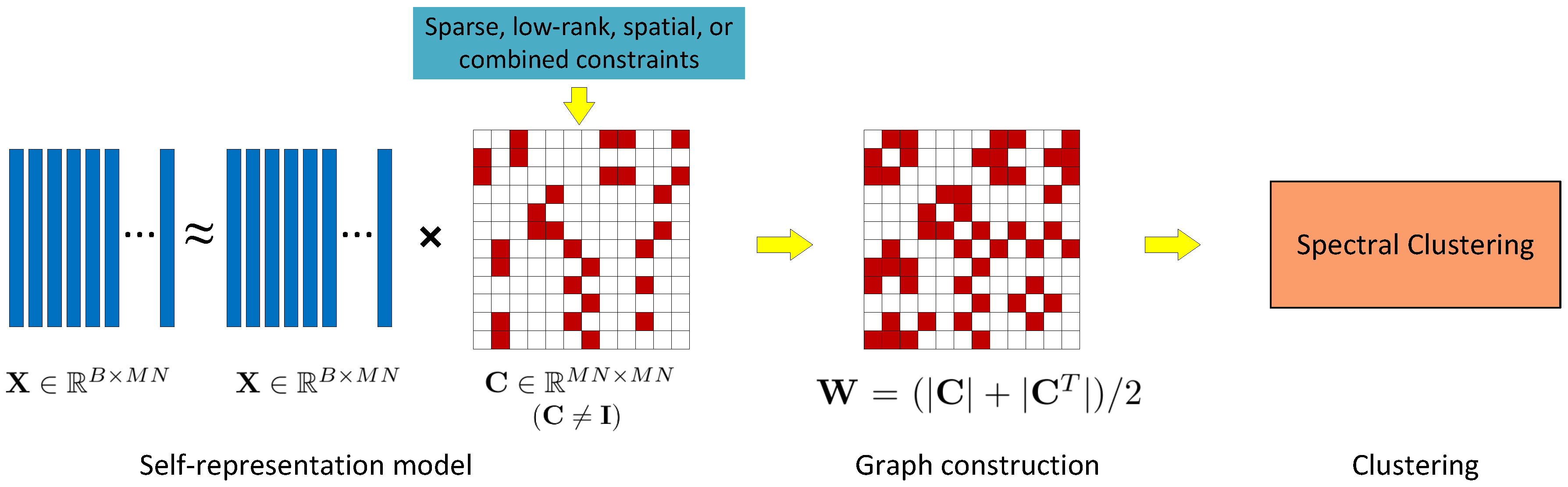
4.1. Self-Representation Based Clustering Methods

Sparse representation is a landmark technique in dealing with high-dimensional data and already achieved great success in signal processing [108,109,110], pattern recognition [111], image processing [112,113,114] and computer vision [115,116]. Basically, it represents input signal by a linear combination of a few atoms from a dictionary. Next to sparse representation, low-rank representation is another successful technique in signal processing which aims to learn a representation of data that has a low-rank property. Recently, both techniques were adopted to learn the similarities between data points within a self-representation framework where the input data were employed as the dictionary.

Self-representation based clustering methods are in fact built on the framework of spectral clustering as shown in Figure 5, where the similarity matrix of a graph, i.e., $\mathbf{W}$, is particularly derived from the coefficients matrix $\mathbf{C}$ that is learned by solving sparse coding or low-rank representation problems with the input data being a dictionary as follows:

$$\begin{array}{c}\underset{\mathbf{C}}{argmin}\mathcal{F}\left(\mathbf{C}\right)+\mathcal{G}\left(\mathbf{E}\right)\mathrm{s}.\mathrm{t}.\mathbf{X}=\mathbf{X}\mathbf{C}+\mathbf{E},\hfill \end{array}$$

(1)

where $\mathcal{F}\left(\mathbf{C}\right)$ is a regularization term with respect to $\mathbf{C}$, which can be a sparse constraint, a low-rank constraint, a smoothing constraint or mixed constraints, $\mathcal{G}\left(\mathbf{E}\right)$ is a function with respect to the error matrix $\mathbf{E}$. Clustering models (1) are often referred to as subspace clustering in the literature with the assumption that data points belonging to the same class are drawn from a linear subspace [37]. Compared with traditional spectral clustering methods where the similarity matrix is often built with a fully connected graph, k nearest neighbours (KNN) graph or $\epsilon$-neighborhood graph, self-representation based methods have the following advantages in general:

• The number of nearest neighbours in the graph is adaptively determined for each data point by sparsity or low-rank constraint in the representation models, which avoids specifying a fixed number of neighbours for all the data points in KNN graph.
• Selecting an effective similarity measurement between data points is difficult in general, especially for high-dimensional data where “curse of dimensionality” problem might be suffered. In the self-representation based models, the representation coefficients matrix is utilized to build a similarity matrix, avoiding thereby the ad-hoc selection of similarity measurements.

We classify self-representation based clustering methods into seven sub-categories: spectral-based, spatial-spectral, object-based, semi-supervised, multi-view, kernel-based and graph learning based methods. Each of them will be introduced in the following subsection.

4.1.1. Spectral-Based Clustering Methods

Sparse subspace clustering (SSC) [31] and low-rank representation (LRR) [43] are two pioneer works of self-representation based clustering methods. Following the framework in Figure 5, SSC obtains a sparse coefficients matrix $\mathbf{C}=[{\mathbf{c}}_1,{\mathbf{c}}_2,\dots ,{\mathbf{c}}_{MN}]$ by solving:

$$\begin{array}{c}\underset{{\mathbf{c}}_i}{argmin}{\parallel {\mathbf{c}}_i\parallel }_0\mathrm{s}.\mathrm{t}.{\mathbf{x}}_i=\mathbf{X}{\mathbf{c}}_i,c_{ii}=0(i=1,2,\dots ,MN),\hfill \end{array}$$

(2)

where $\parallel {\mathbf{c}}_i{\parallel }_0$ represents the number of non-zeros of ${\mathbf{c}}_i$ and $c_{ii}$ is the i-th element of ${\mathbf{c}}_i$. The constraint $c_{ii}=0$ is used to avoid a trial solution of $\mathbf{C}=\mathbf{I}$. Minimizing the sparsity of representation vector ${\mathbf{c}}_i$ with ${\ell }_0$-norm is NP-hard. However, model (2) can be approximately solved by relaxing the ${\ell }_0$-norm to the convex ${\ell }_1$-norm:

$$\begin{array}{c}\underset{{\mathbf{c}}_i}{argmin}{\parallel {\mathbf{c}}_i\parallel }_1\mathrm{s}.\mathrm{t}.{\mathbf{x}}_i=\mathbf{X}{\mathbf{c}}_i,c_{ii}=0,\hfill \end{array}$$

(3)

where $\parallel {\mathbf{c}}_i{\parallel }_1={\sum }_j\left|c_{ij}\right|$. The essential idea of SSC is that among infinitely many possibilities to represent a data point ${\mathbf{x}}_i$ in terms of other points, a sparse representation will select a few points that belong to the same class as ${\mathbf{x}}_i$. Thus, the coefficients matrix $\mathbf{C}$ can be used to build a similarity matrix for the input data points by $\mathbf{W}=\left(\right|\mathbf{C}|+|{\mathbf{C}}^T\left|\right)/2$. By applying the similarity matrix into standard spectral clustering algorithm, one can obtain the clustering results of data.

LRR learns the coefficients matrix $\mathbf{C}$ with a low-rank constraint by solving the optimization problem as follows:

$$\begin{array}{c}\underset{\mathbf{C},\mathbf{E}}{argmin}{\parallel \mathbf{C}\parallel }_{*}+\lambda {\parallel \mathbf{E}\parallel }_{2,1},\mathrm{s}.\mathrm{t}.\mathbf{X}=\mathbf{XC}+\mathbf{E},\hfill \end{array}$$

(4)

where ${\parallel \mathbf{C}\parallel }_{*}$ denotes the nuclear norm of $\mathbf{C}$, i.e., the sum of the singular values of $\mathbf{C}$, whcih is used to regularize the rankness of a matrix, ${\parallel \mathbf{E}\parallel }_{2,1}={\sum }_{j=1}^{MN}\sqrt{{\sum }_{i=1}^B{E}_{ij}^2}$ and $\lambda$ is a parameter to control the balance between different terms. The utilized low-rank constraint makes LRR robust to noise and outliers [43]. Compared with SSC, LRR is more effective in the learning of global structure of data.

Due to the sparse constraint, the solution of SSC sometimes is too sparse, resulting in the over-segmentation of data points within-cluster. Moreover, the performance of LRR will be degraded if the subspaces of data are not independent. To address these issues, Wang et al. [44] combine sparse and low-rank constraints in a unified model, called LRSSC, yielding improved performance over SSC and LRR. The aforementioned models SSC, LRR and LRSSC often utilize relaxed convex norms, i.e., ${\ell }_1$ norm and nuclear norm, to measure the sparsity and rankness of the coefficients matrix. However, the approximated solutions are suboptimal to the original sparse or low-rank constrained optimization problems. In [45], ${\mathrm{S}}_0$/${\mathrm{L}}_0$-LRSSC was proposed by using non-convex $L_0$ quasi-norm ${\parallel \mathbf{C}\parallel }_0$ for the sparsity constraint and Schatten-0 quasi-norm ${\parallel \mathbf{C}\parallel }_{S_0}={\parallel \mathrm{diag}(\Sigma )\parallel }_0$ ($\mathbf{U}\Sigma {\mathbf{V}}^T=\mathbf{C}$ is the singular value decomposition of $\mathbf{C}$) for the low-rank constraint, achieving improved performance compared with LRSSC. Although these methods outperform traditional clustering methods such as k-means and fuzzy c-means in terms of accuracy, they only exploit spectral information of HSI, and neglect spatial dependencies of data points, resulting in a sensitive performance to the spectral variabilities and sparse noise.

4.1.2. Spatial-Spectral Clustering Methods

It has been demonstrated that using spatial information together with spectral information can effectively improve the performance in various HSI processing tasks including supervised classification [117], denoising [118,119,120], change detection [121] and super-resolution [122]. Similarly, incorporating spatial information proves to be beneficial in HSI clustering as well, resulting in a number of spatial-spectral extensions of SSC and LRR in recent years [42,46,48,49,50,51,123,124,125,126]. Spatial-spectral clustering methods take into account spatial information by introducing local constraints on the coefficients matrix or by applying post-processing techniques such as filtering to promote piece-wise smoothness of representation coefficients. As pixels in the local region belong to the same cluster with a high probability, the improved smoothness of coefficients leads to reduced variance within-cluster in the representation/feature domain, which facilitates building a better similarity matrix and thus obtaining an improved accuracy in the standard spectral clustering.

A number of spatial regularizations have been integrated into SSC to promote piece-wise smoothness of the coefficients matrix, which are summarized in

Table 3. Spatial regularizations in spatial-spectral clustering models.

Methods	Spatial Regularization $\mathit{\Psi }\left(\mathit{C}\right)$	Remarks
JSSC [46]	${\sum }_i{\parallel {\mathbf{C}}_i\parallel }_{1,2}$	${\mathbf{C}}_i$ is the coefficients corresponding to the pixels within the i-th super-pixel
SpatSC [47]	${\parallel \mathbf{CH}\parallel }_1$	$\mathbf{H}$ is a difference matrix for 1-D hyperspectral data
L2-SSC [48]	${\sum }_{i=1}^{MN}{\sum }_{j\in {\mathcal{N}}_i}{\parallel {\mathbf{c}}_i-{\mathbf{c}}_j\parallel }_2^2$	${\mathcal{N}}_i$ is the index set of horizontal and vertical neighbours of the i-th pixel
TV-CRC-LAD [32]	${\sum }_{i=1}^{MN}{\sum }_{j\in {\mathcal{N}}_i}{\parallel {\mathbf{c}}_i-{\mathbf{c}}_j\parallel }_1$	${\mathcal{N}}_i$ is the index set of horizontal and vertical neighbours of the i-th pixel
S${}^4$C [42]	$\parallel \mathbf{C}-\overline{\mathbf{C}}{\parallel }_F^2$	$\overline{\mathbf{C}}$ is the smoothed matrix of $\mathbf{C}$ with a 2-D mean filter
S-SSC [49]	$\parallel \mathbf{C}-\overline{\mathbf{C}}{\parallel }_F^2$	$\overline{\mathbf{C}}$ is the smoothed matrix of $\mathbf{C}$ with a 3D median filter
LCR-FLDA [50]	$\mathrm{Tr}\left({\mathbf{CLC}}^T\right)$	$\mathbf{L}$ is the Laplacian matrix of a normal graph
SPHG-LRSC [51]	$\mathrm{Tr}\left({\mathbf{CL}}_H{\mathbf{C}}^T\right)$	${\mathbf{L}}_H$ is the Laplacian matrix of a hypergraph

. Denoting the spatial regularization by $\Psi \left(\mathbf{C}\right)$, the related optimization problems can be represented by a unified form:

$$\begin{array}{cc}\underset{\mathbf{C},\mathbf{E}}{argmin}\Theta \left(\mathbf{C}\right)+\lambda {\parallel \mathbf{E}\parallel }_l+\beta \Psi \left(\mathbf{C}\right),\mathrm{s}.\mathrm{t}.\mathbf{X}=\mathbf{XC}+\mathbf{E},\mathrm{diag}\left(\mathbf{C}\right)=\mathbf{0},\hfill & {\mathbf{C}}^T\mathbf{1}=\mathbf{1},\hfill \end{array}$$

(5)

where $\Theta \left(\mathbf{C}\right)$ is the sparse or low-rank constraint, $\mathrm{diag}\left(\mathbf{C}\right)$ denotes a vector consisting of elements $C_{ii}$ and ${\mathbf{C}}^T\mathbf{1}=\mathbf{1}$ constraint indicates an affine subspace of the data.

Huang et at. [46] take into account spatial dependencies of pixels in the local region by introducing a joint sparsity constraint $\Psi \left(\mathbf{C}\right)={\sum }_i{\parallel {\mathbf{C}}_i\parallel }_{1,2}$, where ${\mathbf{C}}_i\in {\mathbb{R}}^{MN\times N_i}$ is a coefficients matrix of $N_i$ pixels in a local region defined by super-pixel segmentation of HSI and ${\parallel \mathbf{X}\parallel }_{1,2}={\sum }_i\sqrt{{\sum }_j{X}_{ij}^2}$. The utilized ${\ell }_{1,2}$ norm promotes pixels within a super-pixel to select a common set of samples in the subspace representation, resulting in similar coefficients of pixels within a super-pixel. The works in [42,49] develop spatial regularizations with $\Psi \left(\mathbf{C}\right)=\parallel \mathbf{C}-\overline{\mathbf{C}}{\parallel }_F^2$, where $\overline{\mathbf{C}}$ is a smoothed matrix of $\mathbf{C}$ by using smoothing filters, such as 2-D mean filter in [42] and 3D median filter in [49,126]. In [42], 2-D mean filter is applied on each slice of a reshaped 3D coefficients cube $\mathcal{C}\in {\mathbb{R}}^{M\times N\times MN}$, where $\mathcal{C}(:,:,i)\in {\mathbb{R}}^{M\times N}$ is obtained by reshaping each row of matrix $\mathbf{C}$. Compared with the slice-by-slice filtering strategy in [42], a 3D median filter with a 3D moving window is performed on the tensor cube $\mathcal{C}$ in [49,126], which promotes column-wise and row-wise smoothness of $\mathbf{C}$ at the same time.

Instead of approaching a reference matrix obtained by filtering matrix $\mathbf{C}$, total variation (TV) based spatial regularizations are developed to promote similar representations of neighbouring data points. For instance, Guo et al. [47,127] introduce a TV-based regularization, i.e., $\Psi \left(\mathbf{C}\right)={\parallel \mathbf{CH}\parallel }_1$, for 1-D hyperspectral data acquired by spectrometer, where $\mathbf{H}$ is a difference matrix. Zhai et al. [32,48] develop TV-based regularizations, i.e., $\Psi \left(\mathbf{C}\right)={\sum }_{i=1}^{MN}{\sum }_{j\in {\mathcal{N}}_i}{\parallel {\mathbf{c}}_i-{\mathbf{c}}_j\parallel }_l^l(l=1,2)$ for the clustering of HSI, where ${\mathcal{N}}_i$ is the index set of adjacent spatial neighbours of the i-th pixel in horizontal and vertical directions. Minimizing TV-regularized optimization problems in fact facilitates the difference matrices of $\mathbf{C}$ to be sparse, leading to local smoothness of coefficients in the spatial domain. It was demonstrated in [32,47,48,127], by introducing TV-based spatial regularizations clustering accuracy is significantly increased compared with SSC.

Another type of spatial regularization is built on manifold learning with graph Laplacian. By considering each pixel as a graph node, a graph built with input data is utilized to constrain the manifold structure of data in the representation domain to be identical to that in the original data space. Liu et al. [50] introduced a K nearest neighbours (KNN) graph-based spatial constraint $\Psi \left(\mathbf{C}\right)={\sum }_i{\sum }_j{W}_{ij}^{knn}{\parallel {\mathbf{c}}_i-{\mathbf{c}}_j\parallel }_2^2$, where $W_{ij}^{knn}$ measures the similarity between i-th pixel and j-th pixel:

$$\begin{array}{c}{W}_{ij}^{knn}=\left\{\begin{array}{cc}{e}^{-\frac{\parallel {\mathbf{x}}_i-{\mathbf{x}}_j{\parallel }^2}{{\sigma }^2}}\hfill & {\mathbf{x}}_j\in {\mathcal{N}}_i\mathrm{or}{\mathbf{x}}_i\in {\mathcal{N}}_j\hfill \\ 0\hfill & otherwise.\hfill \end{array}\right.\hfill \end{array}$$

(6)

By defining Laplacian matrix by $\mathbf{L}=\mathbf{D}-{\mathbf{W}}^{knn}$, where $\mathbf{D}=\mathrm{diag}\left({\mathbf{W}}^{knn}\mathbf{1}\right)$, the KNN graph-based regularization is reformulated as $\Psi \left(\mathbf{C}\right)=\mathrm{Tr}\left({\mathbf{CLC}}^T\right)$, where $\mathrm{Tr}\left(\mathbf{C}\right)$ is the trace of a real square matrix $\mathbf{C}$, i.e., $\mathrm{Tr}\left(\mathbf{C}\right)={\sum }_i{C}_{ii}$. The graph Laplacian constraint promotes similar pixels to yield similar representation coefficients, facilitating a better similarity matrix and thus leading to an improved clustering accuracy. The normal graph can only model the pair-wise connection of nodes. In fact, one node can have connections with multiple nodes and the connected nodes can be seen as a group. In order to exploit group information in the subspace representation, Xu et al. [51] introduce a hypergraph-based graph regularization, i.e., $\Psi \left(\mathbf{C}\right)=\mathrm{Tr}\left({\mathbf{CL}}_H{\mathbf{C}}^T\right)$, where ${\mathbf{L}}_H$ is a normalized hypergraph Laplacian matrix obtained by:

$$\begin{array}{c}{\mathbf{L}}_H=\mathbf{I}-{\mathbf{D}}_v^{-\frac{1}{2}}\mathbf{H}{\mathbf{W}}_H{\mathbf{D}}_e^{-1}{\mathbf{H}}^T{\mathbf{D}}_v^{-\frac{1}{2}}\hfill \end{array}$$

(7)

with ${\mathbf{D}}_v$ a vertex-degree matrix, ${\mathbf{D}}_e$ a hyperedge-degree matrix, $\mathbf{H}$ an incidence matrix and ${\mathbf{W}}_H$ a weight matrix. We refer to [51] for details. The hypergraph-based regularization constrains the pixels (often more than two) connected by one hyperedge to yield similar representations, yielding thereby better performance than the models using a normal graph. It should be noted that the construction of graphs in [50,51] is highly important, which significantly affects their clustering accuracy.

In [123,128,129], post-processing techniques are developed for LRR or SSC. Different from the aforementioned spatial regularizations, the post-processing step is independent of the optimization problems with respect to $\mathbf{C}$. In [128], a non-local majority voting scheme was proposed, which identifies the cluster of a data point by majority voting with its non-local neighbours, yielding an improved clustering accuracy. In [123], a cascaded weighting and local bilateral filtering scheme is applied on the coefficients matrix of LRR, leading to a better similarity matrix and thus achieving improved clustering results in spectral clustering. In [129], two different strategies, i.e., cosine-Euclidean (CE) and CE dynamic weighting (CEDW), are proposed to build more accurate similarity matrices with the coefficients matrix of SSC. Cosine measure on the sparse coefficients of two pixels is used to exploit spectral information of HSI and Euclidean distance is adopted to incorporate spatial information. Both spectral and spatial information are taken into account in CE and CEDW. In [130], based on the sparse coefficients of SSC, an improved similarity matrix is built by the multiplication of cosine-measured similarity matrix and Gaussian kernel dynamic similarity matrix, incorporating both spatial and spectral information of HSI. In general, post-processing-based clustering approaches have lower computational complexities compared with the spatial regularizations constrained clustering models. However, as the post-processing step is performed on the results of LRR or SSC, the performances of [123,128,129,130] might be significantly degraded when LRR or SSC fails to produce a fair result.

4.1.3. Object-Based Clustering Methods

The aforementioned clustering methods classify HSI pixel-by-pixel, which can be easily affected by impulse noise or outliers. Moreover, due to the huge dictionary in the self-representation models, the computational complexities of these approaches are excessively high, which imposes a severe limitation on large-scale data. To alleviate these problems, object-based clustering methods [52,53] were developed. Compared with pixel-wise clustering approaches, object-based clustering methods require an additional pre-processing step to compress the data size of HSI. Super-pixel segmentation techniques are often applied to achieve this by segmenting HSIs into non-overlapping super-pixels and considering each super-pixel as an “object”. As the pixels within a super-pixel often belong to the same cluster, one can cluster an HSI on the super-pixel level, which significantly reduces the number of data points.

In [52], mean-shift segmentation method [131] is adopted for super-pixel segmentation. Let p be the number of super-pixels or “objects”. Then, reweighed mass centers of the 3D “objects”, denoted by $\overline{\mathbf{X}}=[{\overline{\mathbf{x}}}_1,{\overline{\mathbf{x}}}_2,\dots ,{\overline{\mathbf{x}}}_p]$, are iteratively learned, which serve as input spatial-spectral features of different “objects”. Next, representation coefficients matrix of $\overline{\mathbf{X}}$ is obtained by solving:

$$\begin{array}{c}\underset{\overline{\mathbf{C}},\mathbf{E}}{argmin}\parallel {\mathbf{W}}_e\odot \overline{\mathbf{C}}{\parallel }_1+\frac{\lambda }{2}{\parallel \mathbf{E}\parallel }_F^2\mathrm{s}.\mathrm{t}.\overline{\mathbf{X}}=\overline{\mathbf{X}}\overline{\mathbf{C}}+\mathbf{E},\mathrm{diag}\left(\overline{\mathbf{C}}\right)=\mathbf{0},{\overline{\mathbf{C}}}^T\mathbf{1}=\mathbf{1},\hfill \end{array}$$

(8)

where ${\mathbf{W}}_e$ is a weight matrix to improve the sparsity of $\overline{\mathbf{C}}$ and ⊙ represents element-wise multiplication of two matrices. As the clustering is performed on a super-pixel level, the clustering speed is much faster than the pixel-wise clustering methods.

Wang et al. [53] employ SLIC [132] for the super-pixel segmentation of HSIs. Compared with [52], the correlation between super-pixels is specially taken into account in the subspace representation by introducing a new spatial regularization. The objective function with respect to coefficients matrix $\overline{\mathbf{C}}$ of super-pixels is modelled by

$$\begin{array}{c}\underset{\overline{\mathbf{C}}}{argmin}\parallel \overline{\mathbf{C}}{\parallel }_1+\frac{{\lambda }_1}{2}\parallel \mathbf{S}-\mathbf{S}\overline{\mathbf{C}}{\parallel }_F^2+\frac{{\lambda }_2}{2}{\parallel \overline{\mathbf{C}}-\tilde{\mathbf{C}}\parallel }_F^2\mathrm{s}.\mathrm{t}.\mathrm{diag}\left(\overline{\mathbf{C}}\right)=\mathbf{0},{\overline{\mathbf{C}}}^T\mathbf{1}=\mathbf{1},\hfill \end{array}$$

(9)

where each column of $\mathbf{S}$ is the averaged spectral signature of a super-pixel and $\tilde{\mathbf{C}}$ is an estimated coefficients matrix by KNN neighbours, i.e., ${\tilde{\mathbf{c}}}_i=\frac{1}{d_i}{\sum }_{j\in {\Omega }_i}{\overline{\mathbf{c}}}_j$ with ${\Omega }_i$ the neighborhood of the i-th super-pixel, $d_i={\sum }_{j\in {\Omega }_i}{T}_{ij}$ and $T_{ij}=\exp (-(\parallel {\mathbf{s}}_i-{\mathbf{s}}_j{\parallel }_2^2)/{\sigma }^2)$. By applying similarity matrix $\mathbf{W}=\left(\right|\overline{\mathbf{C}}|+|{\overline{\mathbf{C}}}^T\left|\right)/2$ into spectral clustering, clustering results can be obtained. To alleviate the effect of inaccurate super-pixels segmentation, the authors of [53] further refine the clustering results by a cumulative Markov random field (MRF)-based post-processing method, resulting in improved clustering accuracy.

4.1.4. Semi-Supervised Clustering Methods

Typically, clustering of HSI does not use any labelled data. However, sometimes a few labelled data points might be accessible, which can provide helpful supervised information to guide clustering algorithms to better learn the cluster structure of data. By incorporating supervised information, semi-supervised clustering methods are developed in [54,55,57]. The idea of [54,55] focuses on the refinement of coefficients matrix in self-representation models with supervised information for a more block-diagonal similarity matrix. In [54], a class probability propagation of supervised information based on SSC (CPPSSC) algorithm was proposed, which shares the same form of the objective function in (8). Compared with the object-based clustering model in (8), CPPSSC is a pixel-level clustering approach where the input matrix is $\mathbf{X}$ and ${\mathbf{W}}_e$ is obtained with supervised information. CPPSSC first derives class probabilities of data points by using sparse representation classification [133] with a dictionary constructed by all labelled data. Then the inner product of class probabilities is utilized to measure the similarities of data points, resulting in a supervised weight matrix ${\mathbf{W}}_e$. By imposing the weight matrix on the coefficients matrix, the connectivities of data points can be learned more accurately in sparse coding, facilitating the constructed similarity matrix to be more block-diagonal. Benefiting from the supervised information, the semi-supervised model CPPSSC outperforms unsupervised models such as SSC and S${}^4$C. However, due to the lack of spatial regularization, its performance is sensitive to the amount of labelled data.

In [55], a semi-supervised method, called joint SSC with label information (JSSC-L), was proposed, which incorporates spatial information and label information in a unified model. Specifically, a joint sparsity constraint is introduced to regularize pixels within a super-pixel to select a common set of data points in the subspace representation. To refine the coefficients matrix, the authors exploit available label information to zero the entries of the sparse coefficient matrix, which correspond to the data points from different classes. The objective function of JSSC-L is formulated as follows:

$$\begin{array}{c}\underset{\mathbf{C}}{argmin}\sum _{i=1}^p{w}_i\parallel {\mathbf{C}}_i{\parallel }_{1,2}+\frac{\lambda }{2}{\parallel \mathbf{X}-\mathbf{XC}\parallel }_F^2\mathrm{s}.\mathrm{t}.{\mathbf{C}}^T\mathbf{1}=\mathbf{1},{\mathcal{P}}_{\mathbb{G}}\left(\mathbf{C}\right)=\mathbf{0},\hfill \end{array}$$

(10)

where $w_i$ is the weight for the i-th super-pixel, p is the number of super-pixels, ${\mathcal{P}}_{\mathbb{G}}\left(\mathbf{C}\right)$ is a projection operator that extracts the entries in $\mathbf{C}$ whose indices are in $\mathbb{G}$, and $\mathbb{G}$ is the union of sets $\{i,i\}$ and $\{i,j\}$ where i-th and j-th pixels are labelled pixels from different classes. In order to make full use of labelled information, label propagation within super-pixels is carried out, which significantly increases the amount of labelled data. Compared with the semi-supervised model CPPSSC and other unsupervised models, JSSC-L achieves a significant improvement of accuracy with 1% labelled data.

Different from [54,55], the authors of [56,57] propagate the label information in a graph that is obtained by solving a self-representation model. Let ${\mathbf{X}}_l\in {\mathbb{R}}^{B\times l}$ be the labelled data, ${\mathbf{X}}_u$ be the unlabelled data, $\mathbf{X}=[{\mathbf{X}}_l,{\mathbf{X}}_u]$, ${\mathbf{Y}}_l\in {\mathbb{R}}^{c\times l}$ be the one-hot label matrix of ${\mathbf{X}}_l$ and $\mathbf{F}=[{\mathbf{F}}_l,{\mathbf{F}}_u]$ be the predicted label matrix of $\mathbf{X}$. The objective function of the semi-supervised clustering model, non-negative LRR (NNLRR), in [56,57] is formulated as follows:

$$\begin{array}{cc}\underset{\mathbf{F},\mathbf{C},\mathbf{E}}{argmin}\sum _{i,j}\parallel {\mathbf{f}}_i-\hfill & {\mathbf{f}}_j{\parallel }_2^2{C}_{ij}+{\lambda }_{\infty }\parallel {\mathbf{F}}_l-{\mathbf{Y}}_l{\parallel }_F^2+{\gamma \parallel \mathbf{C}\parallel }_{*}+\beta {\parallel \mathbf{E}\parallel }_{2,1}\hfill \\ \hfill & \mathrm{s}.\mathrm{t}.\mathbf{X}=\mathbf{XC}+\mathbf{E},\mathbf{C}\ge {0,\parallel \mathbf{C}\parallel }_0\le T,\hfill \end{array}$$

(11)

where ${\lambda }_{\infty }$ is a sufficiently large value such that $\parallel {\mathbf{F}}_l-{\mathbf{Y}}_l{\parallel }_F^2=0$ is approximately satisfied. The first two terms propagate the labelled vectors ${\mathbf{Y}}_l$ in a graph with the similarity matrix $\mathbf{C}$. The non-negative constraint, i.e., $\mathbf{C}\ge 0$, is utilized to interpret the learned low-rank and sparse matrix $\mathbf{C}$ as a similarity matrix.

Compared with CPPSSC [54] and JSSC-L [55], NNLRR requires much more labelled data to ensure an effective propagation of labels in the graph. Moreover, because of the lack of spatial constraint in NNLRR, the learned similarity matrix can be easily affected by noise and outliers, leading to a less reliable propagation of labels.

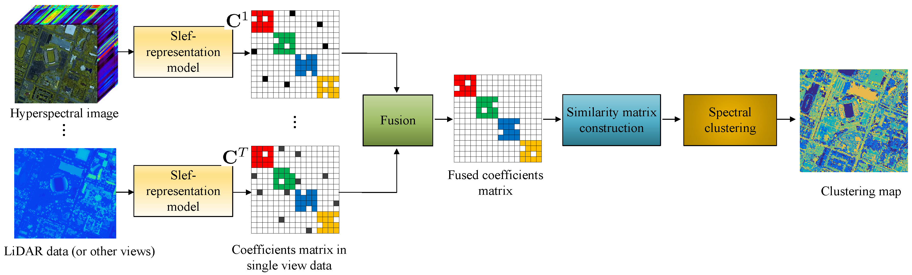
4.1.5. Multi-View Clustering Methods

Multi-view clustering methods, as extensions of aforementioned single-view clustering models, incorporate rich information from different data sources to cluster data points. Here, we refer to different sources acquired by heterogeneous sensors, such as HSI, Light Detection and Ranging (LiDAR) and synthetic-aperture radar (SAR), and features extracted from single-source or multi-source data, such as morphological profiles (MPs) [134], Gabor features [135] and local binary patterns [136], as different views of the same scene. Making use of complementary information from different views can help in discriminating better between data points from different classes. The essential problems of multi-view clustering methods are: (1) how to precisely capture the cluster structure of each view; and (2) how to fuse diverse cluster structures from different views and find a common cluster structure. A flowchart of multi-view clustering methods is shown in Figure 6.

Let ${\{{\mathbf{X}}^t\in {\mathbb{R}}^{B_t\times MN}\}}_{t=1}^T$ denote the multi-view data, where $B_t$ is the dimensionality of the t-th data source and T is the number of data sources. Existing multi-view clustering methods for HSI can be formulated in a unified form:

$$\begin{array}{c}min\sum _{t=1}^T({\lambda }_t\parallel {\mathbf{X}}^t-{\mathbf{X}}^t{\mathbf{C}}^t{\parallel }_F^2+{\beta }_t\mathcal{F}\left({\mathbf{C}}^t\right))+\gamma \mathcal{T}\left({\left\{{\mathbf{C}}^t\right\}}_{t=1}^T\right)\mathrm{s}.\mathrm{t}.\mathrm{diag}\left({\mathbf{C}}^t\right)=\mathbf{0}\left(\mathrm{optional}\right),\hfill \end{array}$$

(12)

where the first two terms are used to learn individual cluster structures within a self-representation model, $\mathcal{F}\left({\mathbf{C}}^t\right)$ is a term consisting of different regularizations and $\mathcal{T}\left({\left\{{\mathbf{C}}^t\right\}}_{t=1}^T\right)$ is a fusion function with respect to ${\left\{{\mathbf{C}}^t\right\}}_{t=1}^T$. In [59,137], a multi-view clustering model was proposed by incorporating polarization information and spectral information of HSIs. Three schemes are designed to capture the individual cluster structure of data with different constraints $\mathcal{F}\left({\mathbf{C}}^t\right)={\parallel {\mathbf{C}}^t\parallel }_1$, $\mathcal{F}\left({\mathbf{C}}^t\right)={\parallel {\mathbf{C}}^t\parallel }_F^2$ or $\mathcal{F}\left({\mathbf{C}}^t\right)={\parallel {\mathbf{C}}^t\parallel }_{*}(t=1,2)$. To fuse cluster structures of the two views, the authors of [59,137] impose a constraint ${\mathbf{C}}^1={\mathbf{C}}^2$, which regularizes the cluster structures learned from different views to be the same.

In [58], a spatial-spectral-based multi-view low-rank SSC (SSMLC) was proposed. It generates spectral views by the partition of spectral bands, spatial views with morphological features and robust views with principle components analysis (PCA). SSMLC learns cluster structures from different views by using sparse and low-rank constraints, i.e., $\mathcal{F}\left({\mathbf{C}}^t\right)=\parallel {\mathbf{C}}^t{\parallel }_1+\alpha {\parallel {\mathbf{C}}^t\parallel }_{*}$, and regularizes the coefficients matrices ${\left\{{\mathbf{C}}^t\right\}}_{t=1}^T$ of different views to be similar with the constraint:

$$\begin{array}{c}\mathcal{T}\left({\left\{{\mathbf{C}}^t\right\}}_{t=1}^T\right)=\sum _{1\le i,j\le t}{\parallel {\mathbf{C}}^i-{\mathbf{C}}^j\parallel }_F^2.\hfill \end{array}$$

(13)

In order to improve the clustering accuracy of SSMLC for the data that is non-linearly separable, the authors of [58] extend SSMLC to a non-linear version with a kernel trick, called K-SSMLC [60]. It learns coefficients matrix in higher dimensional data space with an implicit projection function $\Phi \left({\mathbf{X}}^t\right):{\mathbb{R}}^{B_t}\to {\mathbb{R}}^{{\widehat{B}}_t}$, achieving an improved accuracy compared with SSMLC. Compared with [59,137], which regularizes different views to yield the same coefficients matrix, the constraints across different views in SSMLC and K-SSMLC are more flexible as they allow small deviations of ${\mathbf{C}}^t$ across different views, which is often the case in real data. The disadvantage of [58,59,60,137] is that the learning of view-specific coefficients matrix neglects spatial dependencies of pixels, leading to a sensitive performance to noise and outliers.

In [61], a hybrid-hypergraph regularized multi-view subspace clustering (HMSC) method is put forward, which integrates local and nonlocal spatial information from each view in a unified framework. The authors incorporate the spatial content in each view by developing a hybrid-hypergraph-based manifold constraint $\mathcal{F}\left({\mathbf{C}}^t\right)=\mathrm{Tr}\left({\mathbf{C}}^t{\mathbf{L}}_h^t{\mathbf{C}}^{t^T}\right)$, where ${\mathbf{L}}_h^t$ is the Laplacian matrix of the hybrid-hypergraph consisting of multi-scale local hypergraphs and a nonlocal hypergraph. Moreover, a new decomposition-based scheme was proposed to learn the common intrinsic cluster structure from view-specific subspace representations. The objective function of HMSC is formulated as follows:

$$\begin{array}{c}\begin{array}{cc}\underset{{\mathbf{C}}^t,\mathbf{Z},{\mathbf{E}}^t}{argmin}\sum _{t=1}^T(\parallel {\mathbf{X}}^t-{\mathbf{X}}^t{\mathbf{C}}^t{\parallel }_F^2+\hfill & {\lambda }_1\mathrm{tr}\left({\mathbf{C}}^t{\mathbf{L}}_h^t{\mathbf{C}}^{t^T}\right)+{\lambda }_2\parallel {\mathbf{E}}^t{\parallel }_1)+{\lambda }_3{\parallel \mathbf{Z}\parallel }_{*}\hfill \\ \hfill \mathrm{s}.\mathrm{t}.{\mathbf{C}}^t=& \mathbf{Z}+{\mathbf{E}}^t(\forall t=1,2,\dots ,T),\hfill \end{array}\hfill \end{array}$$

(14)

where the first two terms are used to learn view-specific cluster structures within a self-representation model, and the fused low-rank matrix $\mathbf{Z}$ is shared by all the views with view-specific sparse deviations ${\mathbf{E}}^t$.

Compared with SSMLC and K-SSMLC which integrate a low-rank regularization for each ${\mathbf{C}}^t$, HMSC contains only one low-rank related constraint, obtaining thereby a lower computational complexity. Moreover, as HMSC incorporates local and nonlocal spatial information in each view, it yields a significant accuracy improvement than SSMLC. Multi-view clustering methods often outperform single-view clustering models in terms of accuracy due to the incorporated complementary information from multi-view data. However, multi-view clustering methods require image registration to ensure an identical spatial resolution across different views, and sometimes need to generate hand-crafted “views”. The quality of image registration and generated features can have a significant effect on the clustering accuracy of multi-view models. Moreover, the learning of coefficient matrices for different views significantly increases the computational complexity.

4.1.6. Kernel-Based Clustering Methods

Due to the effect of noise, spectral mixing and poor imaging conditions, the cluster structure of real HSIs can be highly complex, making the acquired data linearly non-separable. To improve the clustering performance of self-representation-based models in real applications, efforts have been made to extend the linear representation, i.e., $\mathbf{X}=\mathbf{XC}$, to non-linear versions by using non-linear mappings. Kernel methods are often exploited to learn the non-linear cluster structure of HSI [62,63,64,65,66,138]. They typically project the raw data into the reproducing kernel Hilbert space $\mathcal{H}$ where the correlation of data points can be more easily learned in the self-representation model. Representative kernel-based clustering models [62,63,64,138] are summarized by:

$$\begin{array}{cc}\underset{\mathbf{C}}{argmin}\parallel \Phi \left(\mathbf{X}\right)-\hfill & {\Phi \left(\mathbf{X}\right)\mathbf{C}\parallel }_F^2+\lambda \Gamma \left(\mathbf{C}\right)\mathrm{s}.\mathrm{t}.\mathrm{diag}\left(\mathbf{C}\right)=\mathbf{0},\hfill \end{array}$$

(15)

where $\Phi (·)$ represents a mapping function that projects raw data $\mathbf{X}$ to a new higher-dimensional feature space $\Phi \left(\mathbf{X}\right)$ and $\Gamma \left(\mathbf{C}\right)$ is a regularization term with respect to $\mathbf{C}$.

Kernel trick is often utilized to avoid an explicit mapping of data. We define kernel function $\kappa :\mathcal{X}\times \mathcal{X}\to \mathbb{R}$ as $\kappa (\mathbf{x},\mathbf{y})=\langle \Phi \left(\mathbf{x}\right),\Phi \left(\mathbf{y}\right)\rangle$, and the positive semidefinite Gram matrix ${\mathbf{K}}_{XX}\in {\mathbb{R}}^{MN\times MN}$ as:

$$\begin{array}{c}{\mathbf{K}}_{XX}(i,j)=\kappa ({\mathbf{x}}_i,{\mathbf{x}}_j)=\langle \Phi \left({\mathbf{x}}_i\right),\Phi \left({\mathbf{x}}_j\right)\rangle .\hfill \end{array}$$

(16)

Then Equation (15) can be reformulated as follows:

$$\begin{array}{cc}\underset{\mathbf{C}}{argmin}\mathrm{Tr}({\mathbf{K}}_{XX} -\hfill & 2{\mathbf{K}}_{XX}\mathbf{C}+{\mathbf{C}}^T{\mathbf{K}}_{XX}\mathbf{C})+\lambda \Gamma \left(\mathbf{C}\right)\mathrm{s}.\mathrm{t}.\mathrm{diag}\left(\mathbf{C}\right)=\mathbf{0}.\hfill \end{array}$$

(17)

In [62,64], a kernel low-rank and sparse subspace clustering (KLRS-SC) was proposed, which learns the correlations of data points within the framework of (17) by imposing joint low-rank and sparse constraints on the representation matrix $\mathbf{C}$. The sparse constraint promotes a sparse graph, which maximizes inter-cluster separation. The low-rank constraint is used to improve the connectivities of data points belonging to the same cluster. The joint constraints enable the model to capture both local and global structures of HSIs, leading to a more block-diagonal structure of similarity matrix in the Hilbert space. In [63,138], a kernel SSC method with spatial maximum pooling operation (KSSC-SMP) was proposed, which extends SSC to a kernel version. Compared with KLRS-SC, KSSC-SMP additionally incorporates spatial information of HSI by a post-processing technique, i.e., max pooling, in the representation domain, producing a more smoothed clustering map.

The acquisition of HSIs is often degraded by numerous factors, including sensor saturation, thermal effects, quantization errors and transmission errors, resulting in different types of noise in HSIs. To alleviate the effect of noise in the clustering of HSIs, Jorge et al. [65] combine a TV-based noise denoising model and the kernel-based clustering model KSSC-SMP in a unified framework. Minimizing the TV-based denoising term results in less noisy data, which facilitates a better clustering performance in KSSC-SMP.

Different from the framework in (17), Cai et al. proposed a more generalized model, called efficient kernel graph convolutional subspace clustering (EKGCSC) [66], by improving the self-representation dictionary with graph convolution. The objective function of EKGCSC is formulated as follows:

$$\begin{array}{c}\underset{\mathbf{C}}{argmin}\parallel \Phi \left(\mathbf{X}\right)-\Phi \left(\mathbf{X}\right)\overline{\mathbf{A}}{\mathbf{C}\parallel }_F^2+\lambda {\parallel \mathbf{C}\parallel }_F^2,\hfill \end{array}$$

(18)

where $\overline{\mathbf{A}}={\tilde{\mathbf{D}}}^{-1/2}({\mathbf{A}}_s+\mathbf{I}){\tilde{\mathbf{D}}}^{-1/2}$ is a normalized similarity matrix with $\tilde{\mathbf{D}}=\mathrm{diag}\left(({\mathbf{A}}_s+\mathbf{I})\mathbf{1}\right)$ and ${\mathbf{A}}_s$ being a similarity matrix. $\Phi \left(\mathbf{X}\right)\overline{\mathbf{A}}\mathbf{C}$ can be viewed as a special linear graph convolution operation in the projected high-dimensional feature space. When $\overline{\mathbf{A}}=\mathbf{I}$, model (18) is reduced to the traditional one in (15). The new dictionary $\Phi \left(\mathbf{X}\right)\overline{\mathbf{A}}$ constructed by graph embedding improve the robustness of EKGCSC to noise. Moreover, the optimization problem (18) can be solved by a closed-form solution, which is more computationally efficient and makes EKGCSC easily implemented and applied in practice.

Kernel-based clustering methods often perform better than linear representation-based clustering methods, which benefit from the increased separability of data points in the projected high-dimensional feature space. However, the selection of a proper kernel function is challenging and it is not guaranteed that in the implicit data space the data lies in a union of linear subspaces. Moreover, kernel-based methods need to calculate a predefined kernel matrix, i.e., ${\mathbf{K}}_{XX}$, which significantly increases the computational complexity.

4.1.7. Graph Learning Based Clustering Methods

Graph embedding, i.e., $\mathrm{Tr}\left({\mathbf{CLC}}^T\right)={\sum }_i{\sum }_j{\parallel {\mathbf{c}}_i-{\mathbf{c}}_j\parallel }_2^2{W}_{ij}$, is an effective technique to preserve local structure of data in the representation domain by promoting similar data points to yield similar coefficients vectors. The construction of the similarity matrix $\mathbf{W}$ is essential in graph embedding. Traditional graph-regularized clustering methods adopt a fixed similarity matrix, which is calculated from the raw data. KNN graph is commonly used as defined in (6). However, noise and outliers in HSIs decrease the quality of the similarity matrix, resulting in an unreliable graph embedding in the representation domain. To solve this problem, graph learning strategy was proposed recently in the self-representation-based clustering models [67,68], which iteratively learns a graph from the representation domain. A basic graph learning model can be formulated as follows:

$$\begin{array}{c}\underset{\mathbf{C},\mathbf{S},\mathbf{E}}{argmin}\sum _i\sum _j{\parallel {\mathbf{Xc}}_i-{\mathbf{Xc}}_j\parallel }_2^2{S}_{ij}+\mathcal{R}(\mathbf{C},\mathbf{E},\mathbf{S})\mathrm{s}.\mathrm{t}.\mathbf{X}=\mathbf{XC}+\mathbf{E},\mathbf{S}\mathbf{1}=\mathbf{1},0\le \mathbf{S}\le 1,\hfill \end{array}$$

(19)

where $\mathbf{S}$ is the adaptive graph and $\mathcal{R}(\mathbf{C},\mathbf{E},\mathbf{S})$ is a set of constraints with respect to $\mathbf{C}$, $\mathbf{E}$ and $\mathbf{S}$.

In [68], a clustering method with dual adaptive graphs learning strategy was proposed. The developed model learns a consensus graph from two adaptive graphs that are derived from the representation domain, i.e., ${\sum }_i{\sum }_j{\parallel {\mathbf{Xc}}_i-{\mathbf{Xc}}_j\parallel }_2^2{S}_{ij}$, and projection domain with locality preserving projection (LPP) [139], respectively. The dual adaptive graphs learning strategy learns similarities of data points from two different domains that are less affected by noise, leading to a more robust clustering performance. In [67], a unified clustering model is developed by combining hypergraph learning and spectral clustering. The proposed model leans a hypergraph with constraint $\mathrm{Tr}\left(\mathbf{XC}{\mathbf{L}}_h{\mathbf{XC}}^T\right)$, where ${\mathbf{L}}_h$ is the Laplacian matrix of a hypergraph, and embeds the learned adaptive hypergraph in spectral clustering. The hypergraph learning and spectral clustering benefit from each other in the alternating optimization algorithm, resulting in improved clustering accuracy.

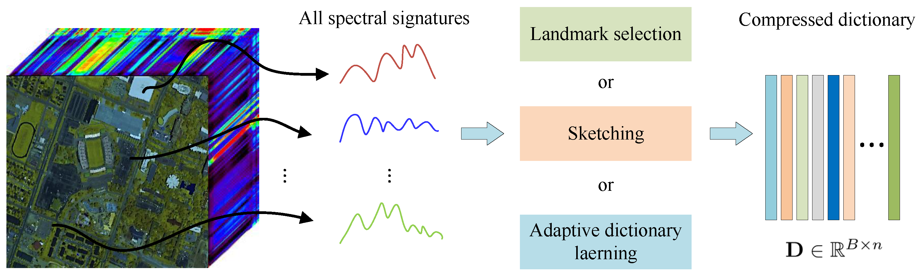
4.2. Dictionary Learning Based Clustering Methods

Self-representation-based clustering models often yield better performance in the clustering of HSI compared with traditional clustering methods such as k-means, fuzzy c-means, density-based clustering methods and spectral clustering. However, as they employ input data as a dictionary, which is typically huge and redundant in practice, the subspace representation is less efficient and less informative. Moreover, the resulting optimization problems are computationally expensive due to the high complexity of $\mathcal{O}\left({\left(MN\right)}^3\right)$, where $MN$ is the total number of pixels in HSI, posing a severe limitation on large-scale data. Recent works [69,70,71,72,73,74,75,76,77,78,79] solve this problem by replacing the self-representation dictionary with a more compact dictionary. Typical ways to obtain the compact dictionary are shown in Figure 7. With a smaller dictionary, the amount of coefficients to be learned is significantly reduced, making the resulting clustering models computationally efficient. Denote the compact dictionary by $\mathbf{D}\in {\mathbb{R}}^{B\times n}$, where n$(n\ll MN)$ is the number of atoms. According to how the dictionary $\mathbf{D}$ is constructed, we classify existing dictionary learning-based clustering methods into three categories: landmark-based, sketch-based and adaptive dictionary-based clustering methods.

4.2.1. Landmark-Based Clustering Methods

This type of method builds the compact dictionary by selecting representative data points from input data. The selected data points are viewed as landmarks of the data, approximately representing the subspaces associated with the input data. The most efficient way to select landmarks is through uniformly random sampling [140]. However, the randomly selected landmarks are often redundant, which requires more data points to represent the input data subspaces, resulting in a larger dictionary. Some methods [69,70] adopt fast clustering algorithms such as k-means to cluster HSI into different groups and obtain landmarks within each group. Another method [71] combines super-pixel segmentation and sparse coding for the selection of landmarks. Those methods typically yield a much smaller dictionary compared with the self-representation dictionary, leading to a more efficient sparse coding problem. After obtaining the coefficients matrix, clustering results can be obtained either by spectral clustering or by designing post-processing techniques, e.g., minimizing reconstruction residuals.

In [70], a landmark-based SSC model with TV regularization (LSSC-TV) was proposed for the clustering of large-scale HSIs. LSSC-TV replaces the self-representation dictionary with a landmark dictionary, which is obtained by over-clustering of HSI with k-means where the centroid of each cluster is collected as a landmark. The size of the landmark dictionary is small, reducing significantly the number of optimization variables compared with self-representation models. Thus, LSSC-TV has lower computational complexity and is more scalable to big data. Moreover, LSSC-TV incorporates spatial information with a TV regularization, which improves the local smoothness of coefficients, leading to improved accuracy. The objective function of LSSC-TV is formulated as follows:

$$\begin{array}{c}\underset{\mathbf{A}}{argmin}\frac{1}{2}{\parallel \mathbf{X}-\mathbf{DA}\parallel }_F^2+{\lambda \parallel \mathbf{A}\parallel }_1+{\lambda }_{tv}\sum _i\sum _{j\in {\mathcal{N}}_i}{\parallel {\mathbf{a}}_i-{\mathbf{a}}_j\parallel }_1\mathrm{s}.\mathrm{t}.\mathbf{A}\ge 0,{\mathbf{A}}^T\mathbf{1}=\mathbf{1},\hfill \end{array}$$

(20)

where $\mathbf{A}\in {\mathbb{R}}^{n\times MN}$ is the sparse coefficients matrix, $\lambda$ and ${\lambda }_{tv}$ are the penalty parameters for the sparsity level and spatial smoothness, respectively, and the non-negative and sum-to-one constraints are used to interpret the coefficients as the probability to select landmarks in the sparse coding. Based on the theory of AnchorGraph in [141], a similarity matrix is constructed by $\mathbf{W}={\mathbf{A}}^T{\Lambda }^{-1}\mathbf{A}$, where $\Lambda \in {\mathbb{R}}^{n\times n}$ is a diagonal matrix with ${\Lambda }_{ii}={\sum }_j{A}_{ij}$. Then, fast spectral clustering algorithm [142] is adopted to obtain the clustering results of HSI, reducing further the computational complexity of LSSC-TV.

Zhai et al. [69] proposed a sparsity-based clustering method for large-scale HSIs. Compared with existing subspace clustering methods, which often rely on spectral clustering to yield clustering results with representation coefficients, the developed clustering methods in [69] use sparse representation recovery residual to cluster HSIs, resulting in a much lower computational complexity. Firstly, a structured dictionary $\mathbf{D}=[{\mathbf{D}}_1,{\mathbf{D}}_2,\dots ,{\mathbf{D}}_c]$ is constructed by using k-means and k-nearest neighbours (KNN) where ${\mathbf{D}}_i$ is a subdictionary corresponding to the i-th cluster that is built by the KNN of the i-th cluster centroid. Inspired by sparse representation classification [133], they obtain discriminative sparse coefficients of all data points by solving a sparsity-based optimization problem, which are further fed into a representation residual-based clustering algorithm to yield clustering results. To reduce the effect of salt-and-pepper noise, a spatial-spectral version, called the joint-sparse-coding-based clustering (JSCC) method, was proposed by introducing an ${\ell }_{1,2}$ norm-based joint sparsity on the coefficients matrix of pixels within a super-pixel, yielding an improved performance in terms of accuracy and time complexity. In [72], a multi-objective SSC was proposed for the clustering of HSIs. A compact dictionary is first constructed by using k-means to reduce the overall computation burden. Different from other subspace clustering methods, which obtain coefficients matrix by solving a single objective function, the authors of [72] simultaneously optimize multiple objective functions, i.e., sparsity term, data fidelity term and spatial TV term, resulting in a parameter-free clustering model.

More recently, Hinojosa et al. develop a computationally efficient clustering method with a small landmark dictionary obtained by super-pixel segmentation and sparse coding [71]. The landmark dictionary enables a fast calculation of sparse coefficients. Spatial filtering is used to post-process the coefficients matrix, promoting the connectivity of neighbouring pixels in the representation domain. To obtain clustering results of large-scale HSIs, fast spectral clustering is applied with the coefficients matrix, reducing further the computational complexity of the clustering method.

4.2.2. Sketch-Based Clustering Methods

Sketch-based clustering methods compress the self-representation dictionary by using a random sketching technique, i.e., $\mathbf{D}=\mathbf{XR}$, where ${\mathbf{R}}^{MN\times n}$ is a random matrix. The compressed dictionary $\mathbf{D}$, referred to as sketched dictionary, is originally developed for computer vision tasks where clustering of faces, digits and scenes is of interest [143]. Same as the landmark dictionary, the size of the sketched dictionary is much smaller than the self-representation dictionary, making the resulting clustering model computationally efficient. It has been theoretically proved that the sketched dictionary is as expressive as the self-representation dictionary with a proper sketching matrix $\mathbf{R}$. Thus, the sketched dictionary can well represent the subspaces associated with the input data. Recent works [73,74,75] apply sketched dictionary in the clustering of HSIs, achieving state-of-the-art performance in terms of efficiency and accuracy. The objective function of sketch-based clustering methods is formulated as

$$\begin{array}{c}\underset{\mathbf{A}}{argmin}\frac{1}{2}{\parallel \mathbf{X}-\mathbf{DA}\parallel }_F^2+\Theta \left(\mathbf{A}\right)+\Psi \left(\mathbf{A}\right),\hfill \end{array}$$

(21)

where $\mathbf{D}=\mathbf{XR}$, $\Theta \left(\mathbf{A}\right)$ is the sparsity or low-rankness related constraints and $\Psi \left(\mathbf{A}\right)$ is a spatial regularization. After obtaining matrix $\mathbf{A}$, KNN graph is built and further fed to spectral clustering to yield clustering results.

In [73], a TV regularized sketch subspace clustering method was proposed for hyperspectral remote sensing images. It adopts Johnson-Lindenstrauss transform to sketch the self-representation dictionary as a compact dictionary, which significantly reduces the number of sparse coefficients to be solved, thereby reducing the overall complexity. In order to alleviate the effect of noise and within-class spectral variations of HSIs, a TV spatial constraint is used on the sparse coefficients matrix, which accounts for the spatial dependencies among the neighbouring pixels. Compared with the traditional SSC model, the sketch-based clustering model obtains significant improvements in accuracy and running speed. Another sketch-based clustering method [75] adopts the same sketching technique of [73,143] to build the compressed dictionary. To better capture the structural information of HSIs in the representation domain, joint sparsity and low-rankness constraints were introduced, which account for the underlying local and global information of HSIs at the same time. Moreover, a nonlocal means regularization is used to incorporate the spatial correlation information, which improves further the clustering accuracy. The objective function of the sketch-based clustering model [75] is shown as follows:

$$\begin{array}{c}\underset{\mathbf{A}}{argmin}\parallel {\mathbf{W}}_a{\odot \mathbf{A}\parallel }_1+{\beta \parallel \mathbf{A}\parallel }_{*}+\frac{\lambda }{2}{\parallel \mathbf{X}-\mathbf{DA}\parallel }_F^2+\frac{\alpha }{2}{\parallel \mathbf{A}-{\overline{\mathbf{A}}}_{NL}\parallel }_F^2,\hfill \end{array}$$

(22)

where ${\mathbf{W}}_a$ is an adaptive weight matrix calculated by $W_{a_{ij}}={\epsilon }_2/(A_{ij}+{\epsilon }_1)$, which leads to an improved sparsity, ${\epsilon }_1$ and ${\epsilon }_2$ are two small constants and ${\overline{\mathbf{A}}}_{NL}$ is a filtered matrix of $\mathbf{A}$ by a nonlocal means filter.

4.2.3. Adaptive Dictionary Based Clustering Methods

Motivated by the success of dictionary learning in signal processing and high- dimensional data analysis [144,145,146,147,148,149], recent works [76,77,78,79] replace the self-representation dictionary with an adaptive dictionary that is leaned from the input data, resulting in computationally efficient clustering models. The developed models often consist of three steps, joint dictionary learning and sparse coding, similarity matrix construction and spectral clustering.

In [76], a novel clustering method based on sparse dictionary learning and anchored regression was proposed. The proposed method first builds a sparse dictionary by multiplying a fixed wavelet dictionary with a learned sparse matrix in a double sparsity constraint-based optimization framework. To improve the efficiency of sparse dictionary learning, an efficient scheme is adopted by using a few randomly selected data points. Then, based on atoms clustering within sparse dictionary and anchored regression, class-specific projection matrices are obtained, which allows a fast calculation of the coefficients matrix. A spatial smoothing filter is applied to the coefficients matrix, which is utilized to build a similarity matrix. Finally, spectral clustering is applied to obtain the clustering results of HSI. The developed model in [76] achieves a low computational complexity. However, the underlying fixed wavelet dictionary might not fit well with the input data. Instead, Bruton et al. [79] proposed an efficient online dictionary learning-based clustering model for HSIs. It obtains a compact dictionary and sparse coefficients simultaneously in a unified model. The learned dictionary is more adaptive to the input data compared with the one in [76]. The sparse coefficients are viewed as extracted features, which are demonstrated to be more discriminative compared with the raw spectral data. The new features facilitate a better similarity matrix, improving thereby the accuracy of spectral clustering. However, only spectral information of HSI is exploited in [79], making the clustering model less robust to the degradations of HSIs.

In [78], a dictionary learning-based clustering method is put forward with an adaptive spatial regularization. Specifically, a weighted joint total variation is formulated by adopting a reweighed ${\ell }_{1,2}$ norm penalty on the difference matrix of coefficients, which encodes effectively the dependencies of spatially neighbouring pixels in the low-dimensional subspaces and promotes the coefficients vectors of neighbouring pixels to be similar. Thus, the variation of data within-cluster is significantly reduced in the representation domain, leading to an improved clustering accuracy in spectral clustering. The objective function of the dictionary learning model is formulated as follows:

$$\begin{array}{c}\underset{\mathbf{D}\ge \mathbf{0},\mathbf{A}}{argmin}\frac{1}{2}{\parallel \mathbf{Y}-\mathbf{DA}\parallel }_F^2+{\lambda \parallel \mathbf{A}\parallel }_1+{\lambda }_{tv}{\parallel {\mathbf{W}}_h{\mathbf{HA}}^T\parallel }_{1,2},\hfill \end{array}$$

(23)

where $\mathbf{D}\ge 0$ requires that the atoms are nonnegative in agreement with the positive spectral intensities of HSIs, $\mathbf{H}$ is a combined TV operator in horizontal and vertical directions and ${\mathbf{W}}_h$ is a diagonal weight matrix for the difference matrix ${\mathbf{HA}}^T$ that is iteratively calculated by using the difference matrix of $\mathbf{A}$. Compared with self-representation models, the complexity of the model in [78] is much lower. Compared with the commonly used TV regularization, the weighted ${\ell }_{1,2}$ norm-based TV promotes row sparsity on the difference matrices of $\mathbf{A}$, preserving better the local spatial structure of HSI in the representation domain. This makes the constructed similarity matrix with representation coefficients more block-diagonal, yielding better results in spectral clustering.

Huang et al. [77] proposed a dictionary learning-based clustering method with a joint sparsity constraint, which accounts for local spatial information of HSIs in the sparse coding. It first segments HSI into nonoverlapping square patches and imposes an ${\ell }_{1,2}$ norm-based constraint on the coefficients matrix of pixels within each patch. Minimizing the joint sparsity constraint promotes selecting a common set of atoms in the sparse coding of similar data points. The objective function of joint sparse coding and dictionary learning is formulated as follows:

$$\begin{array}{c}\underset{\mathbf{D},\mathbf{A}}{argmin}\frac{1}{2}{\parallel \mathbf{Y}-\mathbf{DA}\parallel }_F^2+\sum _{i=1}^s{w}_i{\parallel {\mathbf{A}}_i\parallel }_{1,2},\hfill \end{array}$$

(24)

where s is the number of square patches, ${\mathbf{A}}_i$ is the coefficients matrix of pixels belonging to the i-th patch and ${\left\{w_i\right\}}_{i=1}^s$ are the weights for the joint sparsity constraint. After obtaining coefficients matrix $\mathbf{A}$, different from the work of [78,79], which applies the KNN graph built with $\mathbf{A}$ into spectral clustering to obtain clustering results, the clustering method of [77] adopts a coclustering approach based on a bipartite graph, achieving simultaneous clustering of dictionary atoms and spectral data. An undirected bipartite graph $\mathcal{G}=(\mathbf{D},\mathbf{X},E)$ is built where all dictionary atoms ${\mathbf{d}}_i$ and input data points ${\mathbf{x}}_i$ are viewed as nodes and E represents the edges between nodes. As sparse coefficient $A_{ij}$ represents the correlations between input data point ${\mathbf{x}}_j$ and dictionary atom ${\mathbf{d}}_i$, the adjacent matrix of the bipartite graph $\mathcal{G}$ is built by

$${\mathbf{W}}_b=\left[\begin{array}{cc}\mathbf{0},& \left|\mathbf{A}\right|\\ |{\mathbf{A}}^T|,& \mathbf{0}\end{array}\right]\in {\mathbb{R}}^{(MN+n)\times (MN+n)},$$

(25)

where $\left|\mathbf{A}\right|$ represents the absolute value of $\mathbf{A}$. To obtain clustering results of HSIs, the adjacent matrix of the bipartite graph is applied into normalized cut [150].

In summary, benefiting from the compact dictionaries, the number of variables to be optimized in dictionary learning-based clustering methods is significantly reduced compared with self-representation models, resulting in low computation and memory cost. However, the clustering accuracies of dictionary learning-based clustering methods are sensitive to the built compact dictionary. Moreover, adaptive dictionary-based clustering methods learn the compact dictionary and sparse coefficients simultaneously, leading to non-convex optimization problems where global optimal solutions are not guaranteed. The obtained sub-optimal solutions may degrade the performance of these models.

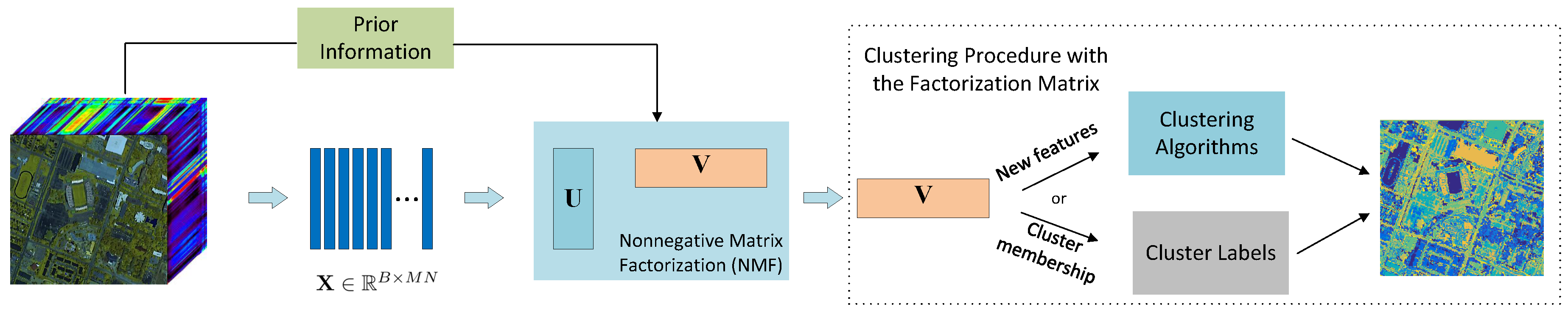
4.3. NMF-Based Clustering Methods

Nonnegative matrix factorization (NMF) [151], which decomposes a nonnegative matrix into the product of two nonnegative factor matrices, has been demonstrated to be an effective tool in many applications including unmixing [152,153,154], source separation [155], compression [156], medical imaging [157], clustering [83,88,158,159,160], etc. For a given nonnegative matrix $\mathbf{X}$, NMF finds two nonnegative matrices $\mathbf{U}\in {\mathbb{R}}^{MN\times r}$ and $\mathbf{V}\in {\mathbb{R}}^{r\times MN}$ such that

$$\begin{array}{c}\mathbf{X}\approx \mathbf{UV}=\sum _{i=1}^r\mathbf{U}(:,i)\mathbf{V}(i,:),\hfill \end{array}$$

(26)

where $\mathbf{U}(:,i)$ is the i-th columns of $\mathbf{U}$ and $\mathbf{V}(i,:)$ is the i-th row of $\mathbf{V}$. In general, NMF is NP-hard and highly ill-posed due to the non-uniqueness of the solutions [161]. Therefore, suitable regularizations are typically introduced to shrink the solution space and to promote additional properties of factorization matrices. The optimization problems of NMF are formulated as

$$\begin{array}{c}\underset{\mathbf{U}\ge 0,\mathbf{V}\ge 0}{argmin}D(\mathbf{X},\mathbf{UV})+\sum _i{\alpha }_i{\Phi }_i(\mathbf{U},\mathbf{V}),\hfill \end{array}$$

(27)

where $D(·,·)$ is a discrepancy term, ${\Phi }_i(·)$ represents the i-th regularization term and ${\alpha }_i\ge 0$ are the regularization parameters to control the influence of ${\Phi }_i(·)$. Typical choices of $D(·,·)$ is Frobenius norm, i.e., ${\parallel ·\parallel }_F^2$, ${\ell }_1$ norm, i.e., ${\parallel ·\parallel }_1$, and ${\ell }_{2,1}$ norm, i.e., ${\parallel ·\parallel }_{2,1}$. For the regularization, ${\ell }_1$ norm, ${\ell }_2$ norm and other smoothing terms are commonly used.

NMF can be used for data clustering in two different ways as shown in Figure 8. The first strategy is to consider NMF as a representation learning technique, where the representation matrix $\mathbf{V}$ is viewed as new features of data. By applying the new features to existing clustering methods, clustering results can be obtained. As normally $r\ll B$ and $r\ll MN$, NMF with $\mathbf{UV}$ is a low-rank approximation of $\mathbf{X}$. Clustering in the feature space can be more effective than that in the raw data space. The second strategy views the factorization matrix $\mathbf{U}$ as a cluster centroids and $\mathbf{V}$ as a cluster membership matrix by setting r to the number of clusters and imposing orthogonal constraint $\mathbf{V}{\mathbf{V}}^T=\mathbf{I}$. This directly obtains clustering results through each column of $\mathbf{V}$. Without other regularization terms, the second strategy is known as orthogonal NMF (ONMF) problems, which is equivalent to a weighted variant of the spherical k-means [162]. Compared with k-means, NMF clustering approaches are more flexible considering that different prior information of data can be easily incorporated by introducing suitable regularizations on the factorization matrices.

The earliest work of NMF-based clustering can date back to 2003 [163], which applies NMF to the clustering of document and obtains superior performance compared with spectral clustering. Subsequent development of NMF-based clustering methods mainly focuses on computer vision tasks and the research on the clustering of HSIs with NMF just appears in recent three years. Depending on whether spatial information is incorporated, we categorize NMF-based clustering approaches of HSIs into spectral-based and spatial-spectral-based methods.

4.3.1. Spectral-Based NMF Clustering Methods

Spectral-based NMF clustering methods treat pixels of HSI independently without considering their spatial dependencies. In [80], a hierarchical clustering method based on rank-two NMF (H2NMF) is put forward. The method starts with a single cluster containing all the data points and performs the following two steps iteratively, (1) cluster selection for further division and (2) split of the selected cluster with rank-two NMF. The major advantage of the method is that the tree-structured clustering results avoid rerunning the algorithms from scratch if the number of clusters required by the user is modified. Compared with k-means, spherical k-means and standard NMF, H2NMF yields better performance in terms of clustering accuracy. In [81], Manning et al. extend H2NMF to a version that supports parallel computing with distributed memory, compute nodes and processors, resulting in a scalable clustering algorithm for big data.

In [82], Fernsel et al. proposed elastic net regularized ONMF clustering models where the factorization rank r is set to the number of clusters. Compared with the traditional NMF, orthogonal constraint $\mathbf{V}{\mathbf{V}}^T=\mathbf{I}$ is introduced for the factorization matrix $\mathbf{V}$, leading to the interpretation of $\mathbf{V}$ as a cluster membership matrix. Moreover, the elastic net regularization with ${\ell }_1$ norm and Frobenius norm is introduced to promote the factorization matrices to be sparse. Specifically, the objective function of the models in [82] is formulated as

$$\begin{array}{c}\underset{\mathbf{U}\ge 0,\mathbf{V}\ge 0}{argmin}D(\mathbf{X},\mathbf{UV})+{\lambda }_U{\parallel \mathbf{U}\parallel }_1+{\mu }_U{\parallel \mathbf{U}\parallel }_F^2+{\lambda }_V{\parallel \mathbf{V}\parallel }_1+{\mu }_V{\parallel \mathbf{V}\parallel }_F^2,\mathrm{s}.\mathrm{t}.\mathbf{V}{\mathbf{V}}^T=\mathbf{I},\hfill \end{array}$$

(28)

where $D(·,·)$ is an ${\ell }_1$ norm or Frobenius norm-based discrepancy term and ${\lambda }_U,{\lambda }_V,{\mu }_U$, ${\mu }_V\ge 0$ are regularization parameters. It has been proved in [82] that the regularized ONMF in fact equals to generalized k-means model with suitable distance measures and centroids.

Different from [80,81,82], which obtain clustering results via asymmetric NMF of the input data, the work of [83] develops a symmetric NMF (SNMF) clustering model for HSI by decomposing data covariance matrix $\mathbf{K}$ as $\mathbf{M}{\mathbf{M}}^T$, where $\mathbf{M}\in {\mathbb{R}}^{MN\times c}$ is a nonnegative matrix and is viewed as a cluster membership matrix. The objective function of SNMF is formulated as

$$\begin{array}{c}\underset{\mathbf{M}\ge 0}{argmin}\parallel \mathbf{K}-{\mathbf{MM}}^T{\parallel }_F^2+\sum _{\rho =1}^{MN}{\lambda }_{\rho }{\parallel \mathbf{M}(\rho ,:)\parallel }_1,\hfill \end{array}$$

(29)

where ${\lambda }_{\rho }$ are the regularization parameters for the sparsity of the rows of $\mathbf{M}$. To solve the non-convex matrix factorization problem (29), the work of [83] converts it to a mixed integer linear programming problem. SNMF is shown to perform better than the standard clustering methods such as k-means and NMF. It should be noted that even compared with supervised classifier such as kernel support vector machine (SVM), which is trained with 25% of labelled data, SNMF often yields far better classification accuracy. However, the computational complexity of SNMF is excessively high, posing limitations on the clustering of large-scale data.

4.3.2. Spatial-Spectral-Based NMF Clustering Methods

Instead of using only the spectral information in [80,81,82,83], spatial information is incorporated in NMF to improve the clustering accuracy [84,85,86,87,88]. In [84], Tian et al. proposed a graph regularized ONMF (GONMF), which employs a graph built in the raw data space to preserve local geometrical structure in the cluster membership matrix. In addition, morphological spatial features of HSIs are extracted and concatenated with spectral data, obtaining more discriminative input data, $\tilde{\mathbf{X}}$, for NMF. The objective function of GONMF is formulated as

$$\begin{array}{c}\underset{\mathbf{U}\ge 0,\mathbf{V}\ge 0}{argmin}{\parallel \tilde{\mathbf{X}}-\mathbf{UV}\parallel }_F^2+\lambda \mathrm{Tr}\left({\mathbf{VLV}}^T\right),\mathrm{s}.\mathrm{t}.{\mathbf{VV}}^T=\mathbf{I}.\hfill \end{array}$$

(30)

GONMF directly obtains clustering results from the cluster membership matrix $\mathbf{V}$. Compared with SSC, GONMF yields improved performance in terms of both accuracy and efficiency. In [85], a similar work to GONMF was proposed, which also takes account of the spatial information of HSIs. Specifically, a total variation regularized spatial constraint is imposed on the cluster membership matrix of ONMF, which promotes neighbouring pixels to be grouped in the same cluster, resulting in improved local homogeneity in the clustering maps.

Zhang et al. [86] proposed a semi-NMF clustering framework of HSIs, which works efficiently on the clustering of large-scale data. Specifically, dimensionality reduction by using orthogonal projection is performed jointly with clustering in a unified framework. The transformed data with dimensionality reduction has a much lower dimension, which facilitates fast clustering of data. To increase the robustness of model to sparse noise and outliers, ${\ell }_{2,1}$ norm is utilized for the loss of dimensionality reduction and semi-NMF clustering. Moreover, a graph Laplacian-based manifold constraint is introduced in the low-dimensional feature space and label space, which promotes similar data points to yield similar features and clustering labels. The objective function of the semi-NMF clustering model is formulated as

$$\begin{array}{cc}\underset{\mathbf{U},\mathbf{V},\mathbf{P},\mathbf{Y}}{argmin}\parallel \mathbf{X}-\mathbf{PY}\hfill & {\parallel }_{2,1}+{\parallel \mathbf{Y}-\mathbf{UV}\parallel }_{2,1}+\alpha (\mathrm{Tr}\left({\mathbf{YLY}}^T\right)+\mathrm{Tr}\left(\mathbf{V}{\mathbf{LV}}^T\right))\hfill \\ \hfill & \mathrm{s}.\mathrm{t}.{\mathbf{P}}^T\mathbf{P}=\mathbf{I},\mathbf{V}{\mathbf{V}}^T=\mathbf{I},\mathbf{V}\ge 0,\hfill \end{array}$$

(31)

where $\mathbf{P}$ is the projection matrix to generate new features of $\mathbf{X}$, i.e., $\mathbf{Y}$, $\mathbf{L}$ is the Laplacian matrix of a similarity matrix and $\mathbf{V}$ is the cluster membership matrix. Note that to improve the scalability of the clustering model (31), only a small portion of pixels in HSI are selected for the input matrix $\mathbf{X}$ and the clustering of the rest pixels is performed by using a KNN classifier according to the clustering results of $\mathbf{X}$. This avoids complicated optimization procedure in (31) for the unselected pixels, making the clustering of HSIs much faster.

It is observed that most NMF-based clustering methods view the factorization matrix $\mathbf{V}$ as a label matrix by setting the factorization rank of NMF to the number of clusters. Although this enables a direct clustering result with $\mathbf{V}$, the linear representation ability of NMF limits their applications on the data that is linearly non-separable. To deal with this problem, in [87] the authors adopt NMF as a feature extraction tool and apply the extracted features to spectral clustering to obtain clustering results. To improve the feature learning in NMF, a graph regularized constraint is introduced in the feature space, which promotes the manifold structures in the raw data space and feature space to be identical. The objective function of the resulting model is shown as follows:

$$\begin{array}{c}\underset{\mathbf{U}\ge 0,\mathbf{V}\ge 0}{argmin}{\parallel \mathbf{X}-\mathbf{UV}\parallel }_F^2+{\lambda }_1{\parallel \mathbf{V}-\mathbf{VZ}\parallel }_F^2,\hfill \end{array}$$

(32)

where $\mathbf{Z}$ is a spectral-spatial similarity matrix that is constructed by using super-pixel segmentation with special attention on exploring intra-superpixel and inter-superpixel connectivities. With the new features $\mathbf{V}$, the similarity matrix of a KNN graph with binary weights $\{0,1\}$ is built, which is further fused with the spectral-spatial similarity matrix $\mathbf{Z}$ by a weighted strategy. The fused similarity matrix is demonstrated to be more block-diagonal, improving thereby the clustering accuracy of spectral clustering.

Recently, a co-clustering approach based on NMF was proposed for the clustering of large-scale HSIs [88], which integrates affinity matrix learning and spectral coclustering into a unified model. Specifically, a joint sparsity regularized sparse representation model was used to learn the correlations between data points and anchors, based upon which a bipartite graph was built as in (25). According to the equivalence between bipartite graph kernel k-means and NMF, a co-clustering module for HSIs and anchors was designed by solving double orthogonal constraints regularized NMF optimization problem. The unified co-clustering model is formulated as follows:

$$\begin{array}{cc}\underset{\mathbf{A},\mathbf{U},\mathbf{V}}{argmin}\stackrel{\mathrm{Co}-\mathrm{clustering} \mathrm{via} \mathrm{NMF}}{\overbrace{{\parallel \mathbf{A}-\mathbf{UV}\parallel }_F^2}}+\hfill & \stackrel{\mathrm{Joint}\mathrm{sparse}\mathrm{coding}\mathrm{within}\mathrm{super}-\mathrm{pixel}}{\overbrace{{\gamma \parallel \mathbf{X}-\mathbf{DA}\parallel }_F^2+\alpha {\sum }_{i=1}^s{\parallel {\mathbf{A}}_s\parallel }_{1,2}}}\hfill \\ \hfill \mathrm{s}.\mathrm{t}.{\mathbf{U}}^T\mathbf{U}=\mathbf{I},& \mathbf{V}{\mathbf{V}}^T=\mathbf{I},\mathbf{U}\ge 0,\mathbf{V}\ge 0,\hfill \end{array}$$

(33)

where $\mathbf{A}$ is the sparse coefficients matrix of $\mathbf{X}$ obtained by joint sparse coding within each super-pixel. Matrix $\mathbf{A}$ can be used to measure the correlations between input data $\mathbf{X}$ and representative anchors, i.e., dictionary $\mathbf{D}$. Benefiting from the ${\ell }_{1,2}$-norm regularized spatial constraint in sparse coding, the coefficients matrix encodes better the correlations between input data and dictionary, leading to a more accurate clustering result in the NMF. In the model (33), the clustering results of $\mathbf{X}$ and $\mathbf{D}$ can be directly obtained via the cluster membership matrices $\mathbf{V}$ and $\mathbf{U}$. Compared with self-representation methods such as SSC and LRR, the co-clustering model via NMF in [88] yields significant improvements in terms of accuracy and computational complexity.

In summary, NMF-based clustering models are more efficient than self-representation-based models as there are much less variables to be optimized. As the factorization matrix $\mathbf{V}$ of NMF indicates the cluster membership of data points, post-processing via other clustering algorithms is not needed, which is different from the aforementioned clustering approaches. According to [164], there are strong correlations between NMF, k-means and spectral clustering such that with mild relaxations of constraints NMF equals to the other two clustering methods. Considering the high flexibility in prior information modelling, low computational complexity and good interpretability, NMF is promising in the clustering of HSIs. However, current research in the field is limited. The disadvantage of NMF is that the related optimization problems are non-convex, which makes their global optimal solutions difficult to be obtained. Moreover, the linear representation ability of NMF limits the clustering performance on the data that are linearly non-separable.

5. Deep Clustering Methods

The model-based clustering methods often require to devise rational constraints according to domain-specific prior information to avoid ill-posed optimization problems. However, the incorporation of prior information highly relies on the experience and domain knowledge of experts, which greatly limits the application of model-based clustering methods. In addition, the added penalty parameters of constraints often vary across different data sets. There is a lack of theoretical guidance to set the parameters adaptively. Moreover, the extracted features by shallow models might not be discriminative enough for clustering especially when dealing with remote sensing images which are often highly complex. Benefiting from the powerful feature extraction capacity, data-driven deep learning technique has achieved great success in a number of applications, including classification [165,166], clustering [167], image denoising [168], spectral unmixing [169] and anomaly detection [170]. However, the research on the clustering of HSIs with deep learning is at a very early stage. This is a new and rapidly emerging domain within the last few years, showing impressive clustering performance and attracting increasing attention and interest in the field [104]. According to the mechanism of feature learning and clustering, current deep learning-based clustering approaches of HSI are categorized into self-representation-based, autoencoder (AE)-based, graph convolution-based and contrastive learning-based methods. Figure 9 shows the main idea of each category.

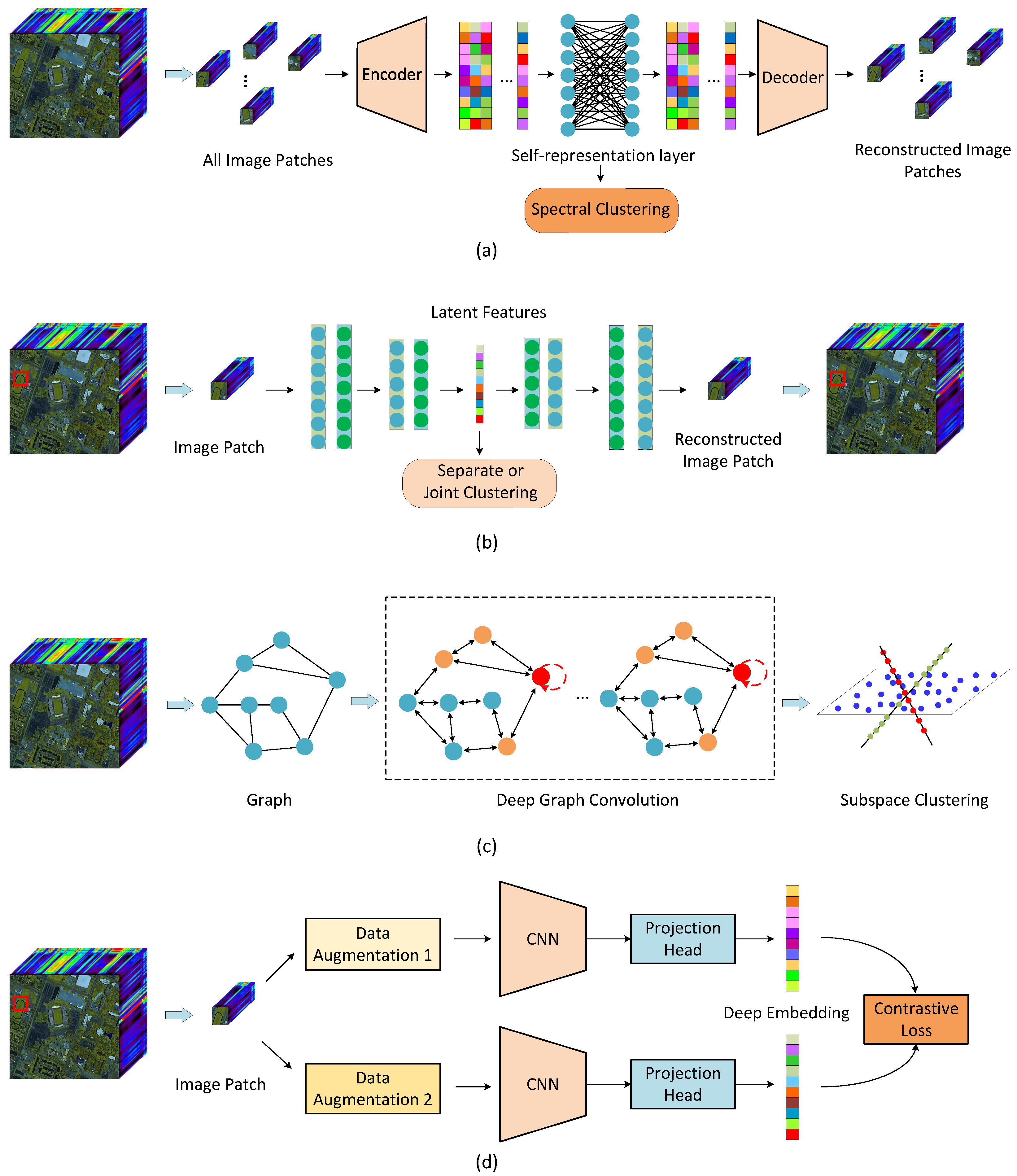
5.1. Self-Representation Based Deep Clustering (SDC)

Basically, SDC methods integrate deep generative neural networks with aforementioned self-representation clustering models, such as SSC [31], and can be seen as the deep versions of the shallow clustering models in Section 4.1. As shown in Figure 9a, AEs are often used to generate latent features, which are expected to be more effective in clustering tasks. The loss of AEs is formulated as

$$\begin{array}{c}{\mathcal{L}}_{AE}={\parallel \mathbf{X}-\overline{\mathbf{X}}\parallel }_F^2+\frac{{\lambda }_1}{2}\Theta \left(\mathbf{Z}\right),\hfill \end{array}$$

(34)

where $\mathbf{X}$ is the input data, $\overline{\mathbf{X}}$ is the reconstructed data by the AEs, $\mathbf{Z}=\mathcal{E}\left(\mathbf{X}\right)$ denotes the latent feature extracted by the encoder $\mathcal{E}(·)$ and $\Theta \left(\mathbf{Z}\right)$ is a regularization term with respect to $\mathbf{Z}$. The encoder of AE is cascaded with a self-representation layer, i.e., $\mathcal{E}\left(\mathbf{X}\right)=\mathcal{E}\left(\mathbf{X}\right)\mathbf{C}$, where $\mathbf{C}$ is the self-representation coefficients matrix. The loss of self-representation layer is formulated as follows:

$$\begin{array}{c}{\mathcal{L}}_{SR}=\frac{{\lambda }_2}{2}{\parallel \mathbf{Z}-\mathbf{ZC}\parallel }_F^2+\frac{{\lambda }_3}{2}\Psi \left(\mathbf{C}\right),\hfill \end{array}$$

(35)

where $\Psi \left(\mathbf{C}\right)$ is a regularization term to avoid trivial solution of $\mathbf{C}=\mathbf{I}$. Combining the reconstruction loss of AE with the loss of self-representation layer, the overall loss function is derived by

$$\begin{array}{c}\mathcal{L}={\mathcal{L}}_{AE}+{\mathcal{L}}_{SR}.\hfill \end{array}$$

(36)

The training of SDC models often consists of two steps: pre-training of AEs by minimizing ${\mathcal{L}}_{AE}$ and fine-tuning step by minimizing (36). Once the coefficients matrix $\mathbf{C}$ is obtained, a similarity matrix can be built as in SSC by $\mathbf{W}=\left(\right|\mathbf{C}|+|{\mathbf{C}}^T\left|\right)/2$. Finally, the similarity matrix is fed into spectral clustering to obtain clustering result.

The first SDC model [89] was proposed in 2017, which introduces a self-representation layer between the encoder and decoder to model the self-expressiveness of data in the nonlinear feature space, achieving remarkable performance in the clustering of faces and objects. Motivated by [89], Laplacian regularized SDC models [90,91,92] were recently proposed for the clustering of HSI, which yield significant improvements compared with the shallow representation-based clustering methods. Basically, graph Laplacian constraint is employed to encode the correlations of data points either in the latent feature space or in the self-representation domain, making the manifold structure of learned features to be more consistent with that in the original domain. In [90], the authors introduced a graph Laplacian-based manifold constraint on the representation coefficients of the self-representation layer to enhance the geometric structure consistency between the input domain and the representation domain. Moreover, skip connections between encoder and decoder are utilized to extract the spatial-spectral information. Experimental results on real data sets show an improved accuracy compared with SDC. The cost function of the model in [90] is formulated as:

$$\begin{array}{c}\frac{1}{2}\parallel \mathbf{X}-\overline{\mathbf{X}}{\parallel }_F^2+\frac{\alpha }{2}{\parallel \mathbf{Z}-\mathbf{ZC}\parallel }_F^2+\frac{\lambda }{2}{\parallel \mathbf{C}\parallel }_P+\frac{\beta }{2}\mathrm{Tr}\left(\mathbf{C}{\mathbf{LC}}^T\right),\mathrm{s}.\mathrm{t}.\mathrm{diag}\left(\mathbf{C}\right)=\mathbf{0},\hfill \end{array}$$

(37)

where $\mathbf{L}$ is the Laplacian matrix of a KNN graph.

In [91], Cai et al. replaced the regular convolutional autoencoder of [90] with a residual convolutional autoencoder, leading to a more easily trained model from scratch. More recently, Cai et al. proposed a hypergraph regularized deep clustering model, called HyperAE [92], which incorporates group structure information of data in the learning of deep latent features. The objection function of HyperAE is formulated as:

$$\begin{array}{c}\frac{1}{2}\parallel \mathbf{X}-\overline{\mathbf{X}}{\parallel }_F^2+\frac{\alpha }{2}{\parallel \mathbf{Z}-\mathbf{ZC}\parallel }_F^2+\frac{\lambda }{2}{\parallel \mathbf{C}\parallel }_F^2+\frac{\beta }{2}\mathrm{Tr}\left(\mathbf{Z}{\mathbf{LZ}}^T\right),\hfill \end{array}$$

(38)

where $\mathbf{Z}$ is the deep latent features of $\mathbf{X}$ and $\mathbf{L}$ is the normalized hypergraph Laplacian matrix. HyperAE is further extended to a semi-supervised version by making use of supervised information from a few labelled data. Specifically, the latent features of AE are fed to a softmax classifier for label prediction, and a cross-entropy-based classification loss is introduced as a task-specific loss function. The cost function of the semi-supervised HyperAE is formulated as:

$$\begin{array}{c}\frac{1}{2}{\parallel \mathbf{X}-\overline{\mathbf{X}}\parallel }_F^2+\frac{\beta }{2}\mathrm{Tr}\left(\mathbf{Z}{\mathbf{LZ}}^T\right)-\frac{\gamma }{2N_l}\sum _{i=1}^{N_l}\sum _{j=1}^c{y}_{ij}\log \left({\overline{y}}_{ij}\right),\hfill \end{array}$$

(39)

where the last term is the cross-entropy loss, $N_l$ is the number of labelled data, ${\mathbf{y}}_i\in {\mathbb{R}}^{1\times c}$ is the one-hot label vector of ${\mathbf{x}}_i$ and ${\overline{\mathbf{y}}}_i$ is the predicted label vector of ${\mathbf{x}}_i$. Benefiting from the hypergraph regularization, the extracted deep latent features of HyperAE are more discriminative than [89], resulting in a better clustering performance both in the unsupervised mode and semi-supervised modes. Recently, Li et al. [93] proposed a mutual information subspace clustering network for the clustering of HSI by embedding contrastive learning and self-representation of data into AE. A contrastive loss, which maximizes the mutual information between input data and latent features, was designed, improving effectively the nonlinear feature learning of data. Experimental results show that the developed model yields improved clustering accuracy compared with other deep clustering approaches.

In [34], a multi-scale SDC model was proposed for the clustering of HSI, which leverages multi-scale convolutional AEs to extract spatial-spectral features of HSI in different scales. By incorporating the self-expressiveness property of features in each scale, the extracted spatial-spectral features are transformed to representation domain and fused further by minimizing the difference of the representation coefficients matrices across all the scales. Although this method obtains improved performance in terms of accuracy, the computational complexity is significantly increased due to the multiple self-representation layers.

Different from previous SDC models which commonly utilize AEs for deep feature extraction, Goel et al. [94] learned discriminative features with deep dictionary learning (DDL), which nonlinearly transforms the input data into a new data space where the data can be separable into different subspaces. The DDL is followed by a self-representation layer where representation coefficients are used to build a similarity matrix for spectral clustering. The objective function of the proposed model in [94] is formulated as:

$$\begin{array}{c}\underset{{\mathbf{D}}_{\mathbf{1}},{\mathbf{D}}_{\mathbf{2}},{\mathbf{D}}_{\mathbf{3}},\mathbf{Z}}{argmin}\stackrel{\mathrm{DDL}}{\overbrace{\parallel \mathbf{X}-{\mathbf{D}}_1{\mathbf{D}}_2{\mathbf{D}}_3{\mathbf{Z}\parallel }_F^2}}+\stackrel{\mathrm{SSC}}{\overbrace{\mu \sum _i\parallel {\mathbf{z}}_i-{\mathbf{Z}}_{i^c}{\mathbf{c}}_i{\parallel }_2^2+\lambda {\parallel {\mathbf{c}}_i\parallel }_1}}\mathrm{s}.\mathrm{t}.\stackrel{\mathrm{ReLU}\mathrm{activation}}{\overbrace{{\mathbf{D}}_2{\mathbf{D}}_3\mathbf{Z}\ge \mathbf{0},{\mathbf{D}}_3\mathbf{Z}\ge \mathbf{0},\mathbf{Z}\ge \mathbf{0}}},\hfill \end{array}$$

(40)

where ${\mathbf{D}}_1,{\mathbf{D}}_2$ and ${\mathbf{D}}_3$ are three layers of dictionaries, $\mathbf{Z}$ is the corresponding representation matrix and ${\mathbf{Z}}_{i^c}$ represents a sub-matrix of $\mathbf{Z}$ by removing ${\mathbf{z}}_i$ in SSC. The experimental results show significant improvement over state-of-the-art clustering methods.

The aforementioned SDC methods separate feature learning from clustering, where the obtained features from deep learning might not be optimal for the clustering task. In [95], a unified self-supervised SDC model combing feature learning and spectral clustering was proposed for the clustering of HSI. It makes use of an AE and a self-representation layer to learn the similarity matrix of data and employs cluster assignments with high confidence from spectral clustering as pseudo-labels to supervise feature learning process. Moreover, a KNN graph built in the original domain is used to guide the initialization of self-expressive coefficient matrix, achieving significant improvement of clustering accuracy. The experimental results in [95] show that the proposed model yields comparable clustering performance to the state-of-the-art supervised deep classification methods with overall accuracy of 97.43%, 100% and 100% on the data sets Indian Pines, Pavia University and Salinas_A, respectively.

Pixel-level self-representation of HSI suffers from high computational complexity and high memory cost in practice, making the aforementioned SDC models on large-scale HSI infeasible. Recently, Cai et al. [96] proposed a super-pixel guided contrastive subspace clustering network (NCSC) for the clustering of large-scale HSIs. By designing a super-pixel pooling autoencoder, the local spatial information of HSI is efficiently encoded, allowing an effective object-level feature extraction. Moreover, contrastive loss, which maximizes the similarity between positive samples generated by KNNs, is introduced to NCSC to promote intra-class similarity of extracted features. Benefiting from super-pixel pooling and contrastive loss, the accuracy and computational cost of NCSC are simultaneously improved, achieving the current state-of-the-art performance in the clustering of HSI.

5.2. AE-Based Deep Clustering (AEDC)

AEDC methods utilize AEs as unsupervised deep data representation to extract latent features for clustering. Due to the nonlinear mapping function of encoders, AEDC is more effective at dealing with complex data compared with traditional linear representation models. Clustering can be performed separately from the latent feature learning, which leads to clustering methods such as those in [97,98,99] consisting of two steps: deep feature learning and clustering. In the first step, reconstruction loss is used to train the AEs. Different types of AEs can be utilized in AEDC, including stacked AE, the traditional AE, convolutional AE and variational AE. With the latent features learned by AEs, classical clustering methods such as k-means and Gaussian mixture models (GMM) are applied to yield clustering results.

A recurrent neural network-based (RNN) asymmetric AE was proposed for the clustering of HSI [97]. The RNN built with long short-term memory (LSTM) or gated recurrent units (GRUs) is utilized as an encoder. By interpreting separate bands of HSI as consecutive steps within a sequence, the high correlation between adjacent bands can be effectively captured by RNN. A multilayer perceptron is utilized as a decoder. With the asymmetric AE, one can obtain a nonlinear mapping function modelled by RNN from input data to latent feature space. The obtained latent features are further fed to GMM to yield clustering results of HSI. As the first attempt to use RNNs in the clustering of HSI, the proposed model in [97] performs comparably to other deep clustering approaches in terms of accuracy, but achieves a faster running speed.

In [98,99], multi-sensor AEDC models were proposed, which make use of rich information from multi-modal remote sensing data, yielding improved clustering performances. Rahimzad et al. [98] developed a boosted convolutional AE with concatenated hand-crafted features as input data for extracting more effective deep features for clustering. Compared with the deep models using raw data as the input of AEs, the network used in [98] is less complex for feature extraction. In [99], Shahi et al. proposed a multi-stream-based AEDC model for the clustering of remote sensing images, consisting of three parallel networks: one spectral network with fully connected AE, one spatial network with convolutional AE, and one fusion network that reconstructs concatenated images. The latent features from spectral and spatial network are concatenated and then fed to k-means clustering algorithm. Experimental results show significant improvement over the traditional SSC and deep learning methods.

The aforementioned AEDC models separate feature learning from clustering, where the extracted features might not be suitable for the clustering task. The works in [33,100,101] integrated deep feature learning and clustering in a unified framework. Apart from the reconstruction loss in AEs, additional clustering loss was introduced to the overall training loss. Representative clustering losses include intraclass distance loss, i.e., k-means loss, and Kullback-Leibler (KL) divergence loss between target distribution and soft assignments. In [100], a deep embedded clustering (DEC) method was proposed. It first pre-trains an AE with reconstruction loss to learn the non-linear mapping function from input data to the latent feature space. Then, the decoder is discarded and the encoder is used for initial feature mapping. By minimizing the KL divergence loss between target distribution and soft assignments, the parameters of encoder and cluster centroids are jointly optimized. DEC yields remarkable improvement over k-means. However, the removal of reconstruction loss in the second fine-tuning stage makes feature extraction via encoder unstable. Nalepa et al. [101] extended DEC by coupling 3D convolutional AEs with clustering and combining reconstruction loss and KL divergence loss in the second fine-tuning stage. Although the AEDC model in [101] yields a high clustering accuracy, the computation time is much longer than others. In [33], an intraclass distance constrained AEDC model was proposed for the clustering of HSI, which performs feature extraction and k-means clustering in a unified model. During the training of network, the clustering error is propagated to the feature learning process of AEs, making the latent features to be more clustering-friendly. The objective function of the model in [33] is formulated as:

$$\begin{array}{c}\underset{{\mathbf{W}}_i,{\mathbf{b}}_i,\mathbf{H},\mathbf{S}}{argmin}\parallel \mathbf{X}-\overline{\mathbf{X}}{\parallel }_F^2+{\lambda }_1{\parallel \mathbf{Z}-\mathbf{HS}\parallel }_F^2+{\lambda }_2\sum _{i=1}^M(\parallel {\mathbf{W}}_i{\parallel }_F^2+\parallel {\mathbf{b}}_i{\parallel }_2^2),\hfill \end{array}$$

(41)

where ${\mathbf{W}}_i$ and ${\mathbf{b}}_i$ are the weights and bias of AE, M is the total number of layers of AE, $\mathbf{Z}$ is the latent features of AE and $\mathbf{H}$ and $\mathbf{S}$ are the cluster centroid matrix and cluster label matrix in k-means, respectively. The second term is k-means clustering loss, which promotes the intraclass distance of data to be smaller in the latent feature space. Experimental results show that the unified model in [33] outperforms both traditional shallow clustering methods and state-of-the-art deep clustering methods.

5.3. Graph Convolution Based Deep Clustering (GCDC)

Graph neural networks extend convolutional neural networks to process the data represented in the graph domain [171]. The feature representation of a node is updated by recursively aggregating representations of its neighbours. GCDC methods integrate graph convolution in the self-representation-based clustering models, which aggregates neighbourhood information of data in the affinity learning, leading to a robust similarity matrix to noise and outliers. Compared with traditional self-representation-based clustering methods, GCDC is more effective in dealing with graph-structured data in the non-Euclidean domain. A typical graph convolution propagation layer [172] can be defined by

$$\begin{array}{c}{\mathbf{X}}^{(r+1)}=\sigma \left(\mathbf{P}{\mathbf{X}}^{\left(r\right)}{\mathbf{W}}^{\left(r\right)}\right),\hfill \end{array}$$

(42)

where ${\mathbf{X}}^{\left(r\right)}$ is the r-the layer’s graph embedding and ${\mathbf{W}}^{\left(r\right)}$ is a weight matrix to be trained, $\mathbf{P}$ is a propagation matrix built with a similarity matrix of input data and $\sigma (·)$ is a non-linear activation function. Cai et al. [66] removed the nonlinear activation function of (42) and employed the graph convolution in the traditional self-representation model, leading to a novel GCDC model as follows:

$$\begin{array}{c}\underset{\mathbf{C}}{argmin}\frac{1}{2}{\parallel \mathbf{X}-\mathbf{XPC}\parallel }_F^2+\frac{\lambda }{2}{\parallel \mathbf{C}\parallel }_F^2,\hfill \end{array}$$

(43)

where the representation matrix $\mathbf{C}$ can be seen as the parameters of a simplified neural network. A closed-form solution of (43) can be obtained, which makes the model computationally efficient and more applicable. Moreover, the model in (43) was extended to a kernel version, which was demonstrated to perform better than existing clustering methods in terms of clustering accuracy.

Zhang et al. [102] replaced the normal graph convolution of (43) with a hypergraph convolution to exploit the group structure of data that is beyond pairwise correlations. Moreover, a multi-hop aggregation strategy with the K power of the propagation matrix, i.e., ${\mathbf{P}}^K$, was employed to incorporate the long-range interdependence between hyperedges and vertices. The resulting model is formulated as

$$\begin{array}{c}\underset{\mathbf{C}}{argmin}\frac{1}{2}\parallel \mathbf{X}-{\mathbf{XP}}_h^k{\mathbf{C}\parallel }_F^2+\frac{\lambda }{2}{\parallel \mathbf{C}\parallel }_F^2,\hfill \end{array}$$

(44)

where ${\mathbf{P}}_h$ is the propagation matrix of a hypergraph and k is the number of hypergraph propagations. The developed model outperforms (43) and achieves state-of-the-art clustering accuracy on five benchmark HSI data sets.

In [103], Cai et al. proposed a more generalized linear graph convolutional network, consisting of a parameter-free neighbourhood propagation and a task-specific linear model with a closed-form solution. As in [102], the non-linear activation function of (42) is removed, resulting in a simplified linear graph convolutional network. Moreover, an improved propagation scheme over [102] was devised by considering the initial node features, which is formulated as:

$$\begin{array}{c}{\mathbf{H}}^{(r+1)}=(1-\alpha ){\mathbf{H}}^{\left(r\right)}\mathbf{P}+\alpha \mathbf{X}\mathrm{s}.\mathrm{t}.{\mathbf{H}}^{\left(1\right)}=\mathbf{X},r=1,\cdots ,K.\hfill \end{array}$$

(45)

It is observed that the initial feature $\mathbf{X}$ also contributes to the update of graph embedding ${\mathbf{H}}^{\left(r\right)}$ with a fixed proportion $\alpha$. By setting $\alpha =0$, the derived propagation matrix of (45) equals to the one in [102]. With the graph propagation scheme (45), a subspace clustering model is formulated as:

$$\begin{array}{c}\underset{\mathbf{C}}{argmin}\frac{1}{2}\parallel \mathbf{X}-{\mathbf{H}}^{(K+1)}{\mathbf{C}\parallel }_F^2+\frac{\lambda }{2}{\parallel \mathbf{C}\parallel }_F^2,\hfill \end{array}$$

(46)

where ${\mathbf{H}}^{(K+1)}$ is the final graph embedding with the linear graph convolution network and $\mathbf{C}$ is the parameter matrix of the overall deep clustering network. Final clustering result can be obtained by applying the affinity matrix $\mathbf{C}$ into spectral clustering. It is demonstrated that the developed model outperforms traditional shallow representation-based methods and deep clustering methods.

5.4. Contrastive Learning Based Deep Clustering (CLDC)

Contrastive learning, as a recent new self-supervised learning technique, has achieved remarkable performance in feature learning [173,174] and classification of HSIs [175,176]. It promotes different augmentations of the same data point, called positive pairs, to yield more similar deep representations compared with the augmentations of other input data points, leading to improved discrimination between data points in the feature space. To achieve this, different contrastive loss functions were designed, including the instance-level InfoNCE loss [177,178] and between-cluster loss [179,180]. Compared with the aforementioned AE-based deep clustering models, which lean features by minimizing data reconstruction loss, contrastive learning is more effective in the learning of discriminative features for classification tasks with contrastive losses. Contrastive learning in the clustering of HSIs is at a very early stage. The initially obtained clustering performance is remarkable and demonstrates that contrastive learning is highly promising in the domain.

In [104], Cao et al. proposed an effective classification framework for HSIs by combining contrastive learning and AEs. It consists of three steps: (1) generations of two augmentations of data by variational AE (VAE) and adversarial AE (AAE), (2) feature extraction via contrastive learning and (3) clustering or classification of the generated deep features. In the first step, two different AEs are employed as transform functions for data augmentation. In the second step, the authors developed an adaptive InfoNCE contrastive loss by incorporating group information of features, promoting the within-cluster features to be close to the centroids. Experimental results show that contrastive learning is able to extract more discriminative features even compared with supervised models. In [105], Kang et al. adopted random patch cropping to generate anchor images and generate augmented images by selecting patches that are close to the central pixels of anchor images. CNNs were employed to extract deep features of anchor images and augmented images. With the InfoNCE contrastive loss, the parameters of CNNs are obtained. Finally, the authors fed the learned features from CNNs into classifiers or clustering algorithms to obtain classification results. In [106], Hu et al. generated augmented images for contrastive learning by image flipping and random removal of non-central pixels. Moreover, a two-branches-based CNN was proposed to extract the spectral and spatial features of HSIs. By combing the instance-level contrastive loss and cluster-level contrastive loss, an overall contrastive learning loss function was obtained, which minimizes the distances between positive pairs and maximizes the distances between negative pairs. Benefiting from the improved discrimination between data points with contrastive learning, the proposed model yields significant accuracy improvement compared with the traditional shallow clustering models and the state-of-the-art deep clustering models.

The aforementioned CLDC models need a separate clustering algorithm, such as k-means or spectral clustering, to cluster the extracted deep features, which makes them unscalable to big data. In [107], Cai et al. developed an end-to-end and scalable CLDC model by combining a symmetric twin CNN-based feature learning neural network with a projection head. The twin CNNs were used to extract deep features of augmented data, which were fed further into the projection head to directly obtain label representation. Moreover, a novel contrastive loss function, consisting of within-cluster contrastive loss and between-cluster contrastive loss, was designed to train the neural network, which promotes a reduction of the within-cluster similarity and an increase of the inter-cluster differences in the feature domain. Experimental results show that the proposed model outperforms the state-of-the-art approaches by large margins.

In general, benefiting from the powerful nonlinear data fitting ability, deep learning-based clustering approaches are more effective for dealing with complex data compared with traditional clustering models. The extracted features by deep learning are often more clustering-friendly, leading to improved clustering accuracy. However, most deep clustering models separate clustering from feature learning, which encounters the problem that the extracted features by deep learning might not fit well with the adopted clustering algorithms. In addition, existing deep clustering methods often need to apply dimensionality reduction techniques to reduce the dimension of HSIs to avoid a high computational complexity. However, this results in the loss of spectral information of HSIs, degrading their clustering accuracy to a certain degree. Moreover, the lack of explainability of deep learning, uninvestigated robustness to noise and high requirement on computing resources pose limitations of deep clustering models in real applications.

6. Experiments

In this section, we conducted extensive experiments with different clustering algorithms on two real HSIs to investigate their clustering performance. Systematic comparisons between different methods and deep analysis were provided. A toolbox that contains the implementations of different clustering methods can be accessed via https://github.com/shhuang-1767/HSI_clustering.git (accessed on 20 May 2023).

6.1. Data Sets

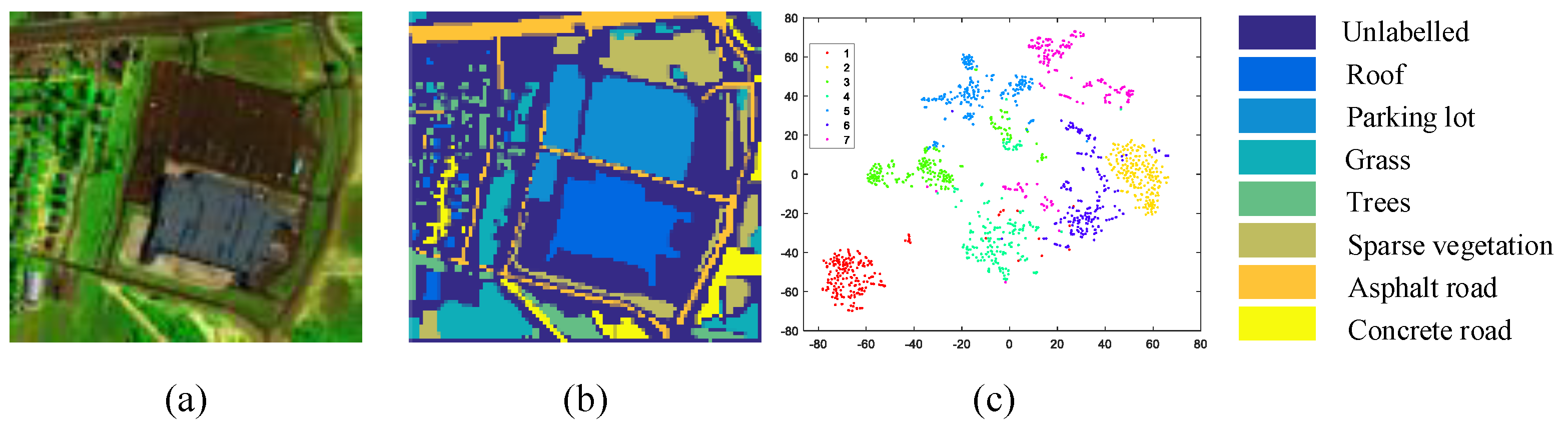
6.1.1. HYDICE Urban

The first data set we used for evaluation was HYDICE Urban, which was captured by Hyperspectral Digital Imagery Collection Experiment (HYDICE) during a flight campaign over Copperas Cove, near Fort Hood, TX, USA. The data size of HYDICE Urban is $307\times 307\times 210$, which captures spectral information from 400 nm to 2500 nm. Due to the serious degradation by atmosphere and water absorption, the bands 1–4, 76, 87, 101–111, 136–153 and 198–210 are removed and the remaining 162 bands are used in the experiments. For computational efficiency, a typical subset of data with a size of $150\times 160\times 162$ was used as the test data, which included seven classes as shown in

Table 4. The classes in the data sets HYDICE Urban and University of Houston.

No.	HYDICE Urban	University of Houston
1	Roof	Concrete
2	Parking lot	Grass-1
3	Grass	Grass-2
4	Trees	Parking lot
5	Sparse vegetation	Roof
6	Asphalt road	Trees
7	Concrete road	Asphalt

. The false-color image and ground truth are shown in Figure 10.

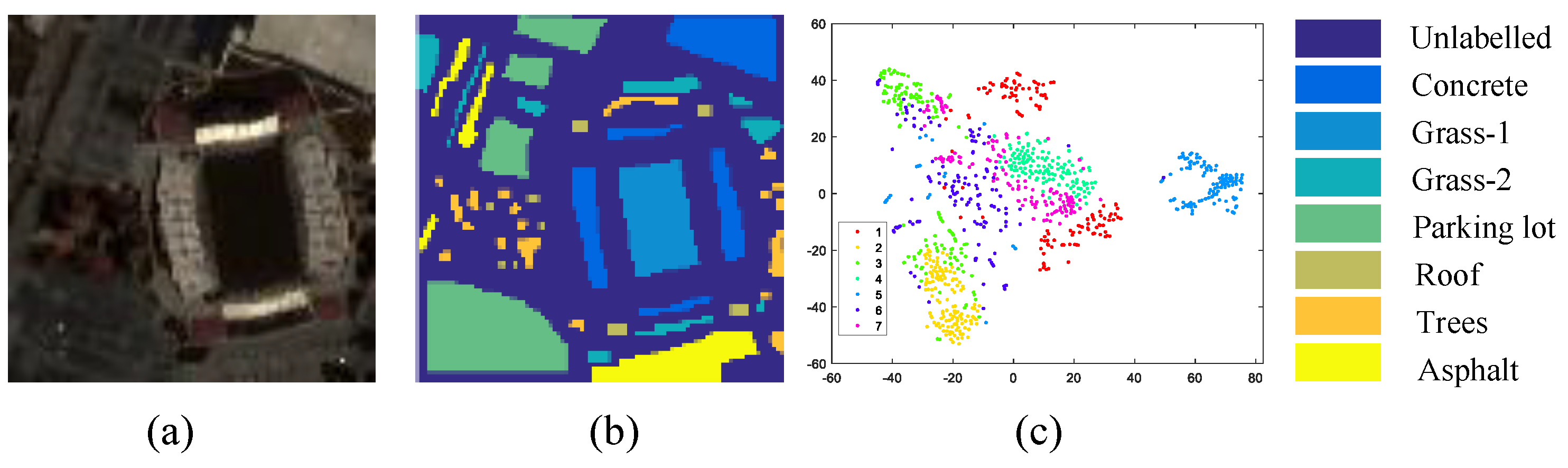
6.1.2. University of Houston (Houston)

The second benchmark data set was acquired by the ITRES-CASI 1500 sensor over the University of Houston campus and the neighbouring urban area. A representative region with the image size of $130\times 130\times 144$ was selected as the test data, which contains seven classes as shown in Table 4. The false-color image and the ground truth of Houston are shown in Figure 11.

6.2. Compared Methods

We selected twelve representative clustering methods for experiments, including seven shallow clustering models, i.e., k-means [19], NMF [36], ONMF-TV [85], SSC [31], JSSC [55], ODL [79] and Sketch-TV [73] and five recent deep learning-based clustering models, i.e., GCSC [66], AEC [100], DEC [100], RNNC [97] and HyperAE [92]. The source codes provided by the authors are used in the experiments. All related parameters were carefully tuned to yield the best overall accuracy. A detailed introduction of the compared methods is given as follows:

• K-means [19]: a commonly used clustering algorithm due to its simplicity and efficiency.
• NMF [36]: a classical clustering method based on NMF.
• ONMF-TV [85]: a spatial-spectral NMF clustering method which integrates orthogonal constraint and TV spatial regularization.
• SSC [31]: a self-representation-based subspace clustering model with a sparsity constraint.
• JSSC [55]: a spatial-spectral SSC model with joint sparsity on the coefficients of segmented super-pixels.
• ODL [79]: a scalable subspace clustering model with online dictionary learning.
• Sketch-TV [73]: a scalable spatial-spectral subspace clustering model by integrating dictionary sketching and a TV spatial regularization.
• GCSC [66]: a graph convolution-based subspace clustering model.
• AEC [100]: an autoencoder-based clustering model where a three-layers stacked denoising AE was used to extract deep features of HSI and k-means was adopted to obtain the final clustering result.
• DEC [100]: a symmetric AE-based deep clustering model, which is an extended version of AEC by introducing a KL divergence clustering loss to jointly learn the encoder and cluster centroids.
• RNNC [97]: an asymmetric AE-based clustering model where recurrent neural nets (RNNs) are employed to build the encoder and a multilayer perceptron was used as the decoder. In our experiments, RNNs were built with long short-term memory (LSTM). The extracted latent features by the encoder of RNNC were fed to k-means to yield clustering results.
• HyperAE [92]: a recent self-representation-based deep clustering model, which integrates the self-expressiveness of data points and graph-based manifold regularization in the autoencoder, resulting in an improved similarity matrix for spectral clustering.

6.3. Evaluation Metrics

We adopt six evaluation metrics to measure the performance of clustering methods, including overall accuracy (OA), average accuracy (AA), Kappa coefficient ($\kappa$), normalized mutual information (NMI), adjusted rand index (ARI) and Purity. To calculate OA, AA and $\kappa$, we first find the best match between the clustering results and ground truth by an optimal mapping function obtained by the Kuhn-Munkres algorithm [181]. For a data set with N samples, the OA is obtained by:

$$\begin{array}{c}\mathrm{OA}=\frac{1}{N}\sum _{i=1}^N\delta (\mathrm{map}\left(r_i\right),l_i),\hfill \end{array}$$

(47)

where $r_i$ is the label of the i-th data point obtained by clustering and $l_i$ is the corresponding true label, $\delta (x,y)=1$ if $x=y$ and is zero otherwise; $\mathrm{map}(·)$ is a mapping function obtained by [181]. Let $n_{i,j}$ be the number of samples in class i that are labelled as class j. The accuracy of the i-th class is computed by $p_i=n_{i,i}/n_{i,+}$, where $n_{i,+}={\sum }_j{n}_{i,j}$ is the number of samples in class i. Then, AA is calculated by

$$\begin{array}{c}\mathrm{AA}=\frac{1}{C}\sum _{i=1}^C{p}_i,\hfill \end{array}$$

(48)

where C is the number of clusters. The Kappa coefficient $\kappa$ is defined as:

$$\begin{array}{c}\kappa =\frac{\frac{1}{N}{\sum }_i{n}_{i,i}-\frac{1}{N^2}{\sum }_i{n}_{i,+}{n}_{+,i}}{1-\frac{1}{N^2}{\sum }_i{n}_{i,+}{n}_{+,i}},\hfill \end{array}$$

(49)

where $n_{+,i}={\sum }_j{n}_{j,i}$ is the number of samples that are identified as class i. The NMI score is calculated as:

$$\begin{array}{c}\mathrm{NMI}=\frac{\mathrm{I}(l;r)}{max\left(\mathrm{H}\right(l),\mathrm{H}(r\left)\right)},\hfill \end{array}$$

(50)

where I$(l;r)$ denotes the mutual information between l and r, and H$\left(l\right)$ and H$\left(r\right)$ are their entropies. The ARI score is obtained by:

$$\begin{array}{c}\mathrm{ARI}=\frac{{\sum }_i{\sum }_j\left(\genfrac{}{}{0pt}{}{n_{i,j}}{2}\right)-\left({\sum }_i\left(\genfrac{}{}{0pt}{}{n_{i,+}}{2}\right){\sum }_j\left(\genfrac{}{}{0pt}{}{n_{+,j}}{2}\right)\right)/\left(\genfrac{}{}{0pt}{}{N}{2}\right)}{\frac{1}{2}({\sum }_i\left(\genfrac{}{}{0pt}{}{n_{i,+}}{2}\right)+{\sum }_j\left(\genfrac{}{}{0pt}{}{n_{j,+}}{2}\right))-\left({\sum }_i\left(\genfrac{}{}{0pt}{}{n_{i,+}}{2}\right){\sum }_j\left(\genfrac{}{}{0pt}{}{n_{+,j}}{2}\right)\right)/\left(\genfrac{}{}{0pt}{}{N}{2}\right)}.\hfill \end{array}$$

(51)

Let $\Omega =\{{\mathbf{w}}_1,{\mathbf{w}}_2,\dots ,{\mathbf{w}}_K\}$ be the clusters obtained by the clustering algorithm and $\mathbb{C}=\{{\mathbf{c}}_1,{\mathbf{c}}_2,\dots ,{\mathbf{c}}_C\}$ be the ground truth, where ${\mathbf{w}}_i$ is the set of samples that are grouped into the i-th cluster and ${\mathbf{c}}_i$ is the set of samples belonging to the i-th cluster according to the ground truth. In the experiments, we assumed that the number of clusters is known, which means $K=C$. Then, the Purity score is obtained by

$$\begin{array}{c}\mathrm{Purity}=\frac{1}{N}\sum _{k=1}^C\underset{j}{max}|{\mathbf{w}}_k\cap {\mathbf{c}}_j|.\hfill \end{array}$$

(52)

The evaluation metric ranges between $[-1,1]$ for $\kappa$, $[0,1]$ for NMI, $[-1,1]$ for ARI and $[0,1]$ for Purity. A larger value indicates a better performance. We also report the running time of different clustering methods. Note that k-means, NMF, NMF-TV, SSC, JSSC and Sketch-TV are implemented in MATLAB on a computer with an Intel core-i7 3930K CPU with 64 GB of RAM. The ODL and GCSC methods are implemented in Python on a server’s node with an Intel core-i7 4930K CPU with 64 GB of RAM. The AEC, DEC, RNNC and HyperAE are implemented in python and run on NVIDIA GeForce GTX 1080Ti with 11 GB of RAM.

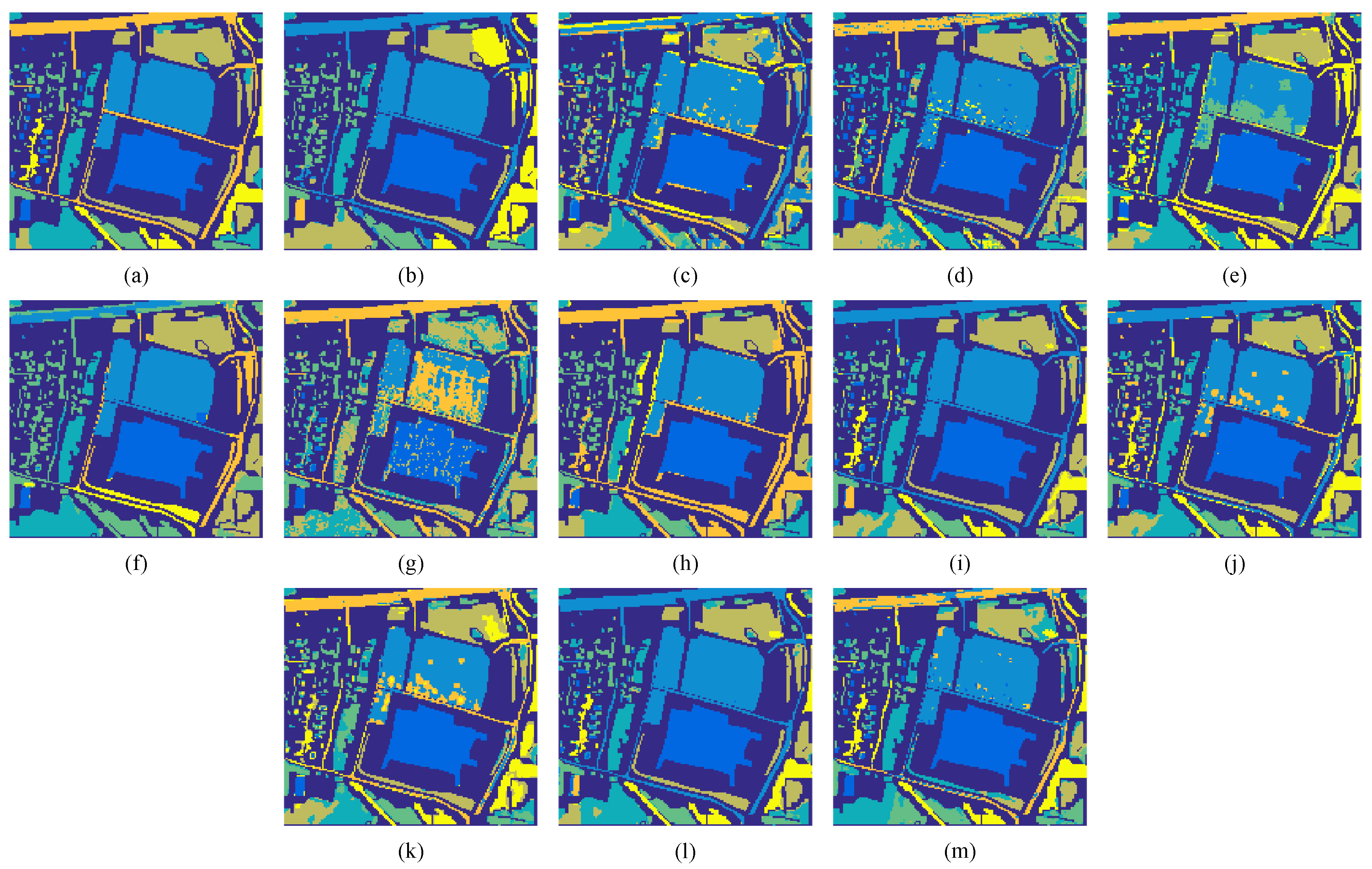
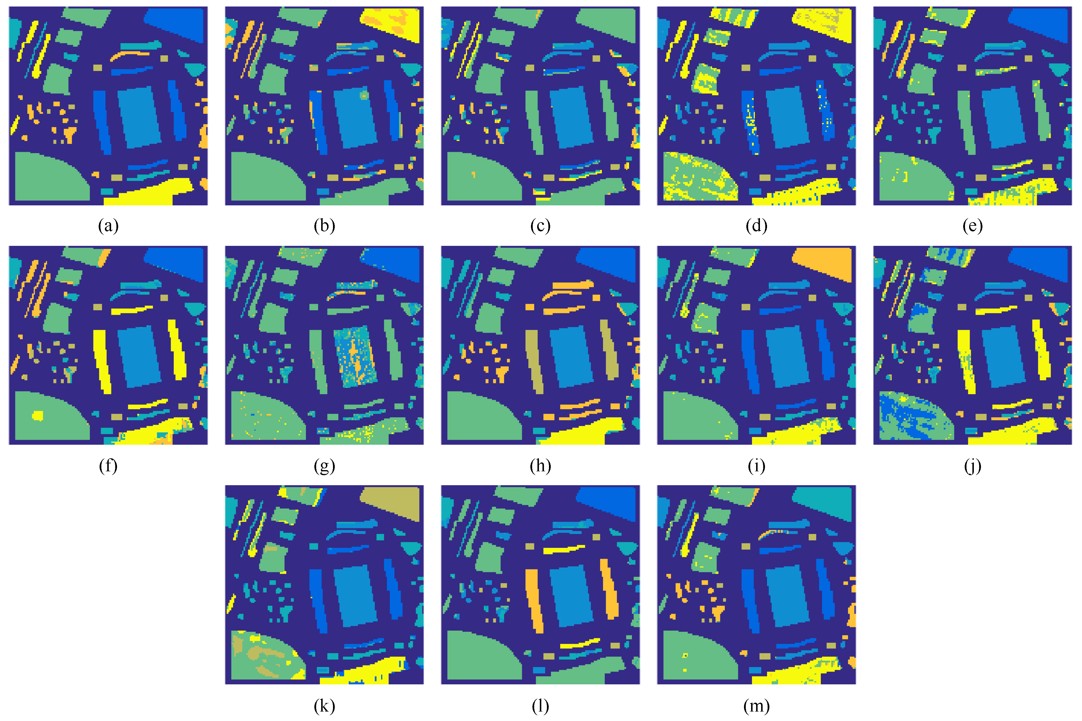
6.4. Performance Comparison

We report the quantitative evaluation of clustering methods on the two data sets in

Table 5. Quantitative evaluation of different clustering methods on the data set HYDICE Urban *.

No.	Shallow Models							Deep Models
	k-Means	NMF	ONMF-TV	SSC	JSSC	ODL	Sketch-TV	GCSC	AEC	DEC	RNNC	HyperAE
1	87.07	87.30	98.94	86.15	90.83	82.96	89.00	93.15	91.70	91.55	92.37	97.64
2	100.00	90.37	93.17	68.87	97.72	48.12	94.80	100.00	89.38	84.45	99.96	95.68
3	39.27	72.56	67.81	85.44	72.97	47.74	67.34	60.73	79.64	55.97	84.63	67.69
4	94.41	46.89	0	1.76	89.54	89.03	91.30	91.93	77.64	82.09	85.51	77.95
5	56.44	65.21	95.69	75.83	67.00	68.84	66.21	99.00	94.06	78.56	97.69	59.96
6	0	22.56	53.04	51.74	24.62	81.13	91.59	0	6.02	72.72	0	59.22
7	62.86	2.88	28.60	80.38	0	0	0.22	84.37	89.80	83.92	92.68	99.00
OA	63.67	62.91	72.49	68.17	68.98	62.06	77.51	75.92	75.46	78.64	79.10	79.61
AA	62.86	55.40	62.46	64.31	63.24	59.69	71.50	75.60	75.46	78.47	78.98	79.59
$\kappa$	0.5665	0.5528	0.6696	0.6277	0.6322	0.5514	0.7325	0.7100	0.7068	0.7484	0.7485	0.7582
NMI	0.6341	0.5111	0.6928	0.6338	0.6175	0.5273	0.7022	0.7746	0.7284	0.6893	0.7865	0.7321
ARI	0.5290	0.4344	0.6326	0.5447	0.5754	0.4100	0.6409	0.6472	0.6416	0.6337	0.6848	0.6619
Purity	0.6630	0.6507	0.7436	0.7443	0.7104	0.6216	0.7841	0.7648	0.7683	0.7864	0.7952	0.7961
Time	3	1	12	3997	8518	190	37	283	422	476	136	1029

* Note: The best result is marked in bold and the second best result is underlined.

and

Table 6. Quantitative evaluation of different clustering methods on the data set Houston *.

No.	Shallow Models							Deep Models
	k-Means	NMF	ONMF-TV	SSC	JSSC	ODL	Sketch-TV	GCSC	AEC	DEC	RNNC	HyperAE
1	47.99	8.12	48.66	46.57	45.90	45.31	46.50	53.50	46.42	52.01	46.50	53.50
2	96.41	99.88	100.00	9.18	99.77	43.34	100.00	100.00	100.00	100.00	100.00	100.00
3	27.42	25.81	10.57	86.20	78.85	54.30	63.08	56.45	46.42	78.85	65.59	0
4	99.75	99.25	65.00	92.36	94.36	97.40	99.85	96.66	64.90	76.24	99.90	97.10
5	76.92	92.31	100.00	77.69	100.00	0	0	100.00	92.31	0	100.00	100.00
6	27.36	33.17	0	0.24	18.64	9.69	68.04	0	25.42	0	0	87.65
7	0	11.57	94.09	0.75	49.18	8.05	68.30	68.30	76.35	80.5	0	75.72
OA	62.91	56.55	61.52	72.03	72.17	54.72	76.39	73.80	63.52	68.28	65.27	75.69
AA	53.69	52.87	59.76	66.14	69.53	36.87	63.68	67.84	64.55	55.37	58.86	73.43
$\kappa$	0.5180	0.4169	0.5296	0.6425	0.6567	0.3882	0.7101	0.6721	0.5491	0.6157	0.5513	0.6953
NMI	0.5904	0.5706	0.5945	0.6498	0.7129	0.3985	0.7864	0.7710	0.5942	0.6693	0.7171	0.8067
ARI	0.5089	0.3811	0.4078	0.5459	0.7178	0.2569	0.7827	0.7125	0.4639	0.5921	0.5717	0.7374
Purity	0.7187	0.5685	0.6171	0.7448	0.8096	0.5686	0.8568	0.8403	0.6473	0.7846	0.7703	0.8591
Time	2	1	6	735	3098	191	29	91	207	267	116	210

* Note: The best result is marked in bold and the second best result is underlined.

and the corresponding clustering maps in Figure 12 and Figure 13. In the tables, the best result is annotated in bold and the second best result is underlined. We set the number of columns of $\mathbf{U}$, i.e., r, to C for NMF and ONMF-TV, the dictionary size to 70 for Sketch-TV, the dimensionality of latent feature to C for AEC and DEC and the dimensionality of latent feature to 18 for RNNC. For all the methods, we first performed PCA [182] to reduce the spectral dimensionality of HSI to eight for computational efficiency and then extract the spatial patch of each central pixel cross all the bands with a $3\times 3$ square window, which serves as the input data point of each clustering method.

It is observed in Table 5 and Table 6 that k-means and NMF do not perform well on both data sets in terms of accuracy. The reason can be attributed to the non-spherical cluster distribution of HSI as shown in Figure 10c and Figure 11c, which cannot be effectively handled by k-means. NMF performs clustering via k-means in a representation domain. However, the representation of pixels are learned independently from each other, making NMF sensitive to noise and outliers. Moreover, the representation learned via NMF is separated from k-means, which might obtain unmatched features for k-means, leading to degraded clustering accuracy. In terms of running time, NMF and k-means are much faster than others, demonstrating their superior efficiency. The results in Table 5 and Table 6 show that ONMF-TV outperforms NMF by a large margin with OA improvements of 9.58% on HYDICE Urban and 4.97% on Houston. The improved performance mainly benefits from the orthogonal constraint and the incorporation of spatial information.

NMF performs similarly to k-means on the data set HYDICE Urban, but much worse than k-means on the data set Houston. This might be caused by the small value of r in NMF, which resulting in non-discriminative features for clustering. Sparse representation-based clustering methods SSC and JSSC perform consistently better than the classic methods k-means and NMF. Compared with k-means-based methods, SSC and JSSC do not assume the cluster distribution of data. Particularly, they uncover the cluster structure of HSI in a graph, which is adaptively learned in a sparsity-driven self-representation model. The results demonstrate that self-representation models are very effective in the learning of cluster structure of complex data. However, the high computational complexity of SSC and JSSC makes their running time much longer than others. The spatial-spectral JSSC method yields higher accuracy than SSC. However, due to the imprecise super-pixel segmentation of HSI, the accuracy improvement of JSSC is rather limited. Compared with SSC, the clustering maps of JSSC are smoother, as shown in Figure 12 and Figure 13. Scalable subspace clustering methods ODL and Sketch-TV obtain much faster running speeds compared with SSC and JSSC due to the introduced compact dictionary, which significantly reduces the amount of parameters to be optimized. However, the running speed improvement of ODL is at the cost of accuracy. Due to the incorporation of spatial information of HSI, Sketch-TV yields improvement both in accuracy and running speed. Among shallow representation-based clustering methods, Sketch-TV performs the best in terms of OA, $\kappa$, NMI, ARI, and Purity. The main reason can be attributed to the reduced feature variance within clusters caused by the adopted TV-based local spatial constraint. Compared with JSSC, which also incorporates spatial information of HSI, Sketch-TV performs considerably better, indicating the importance of an effective spatial constraint.

Deep learning-based clustering methods GCSC, AEC, DEC, RNNC and HyperAE outperform the shallow clustering methods in most cases on the data set HYDICE Urban. On the data set Houston, deep learning-based methods do not consistently yield better performance than the shallow methods. HyperAE performs the best in terms of accuracy among the deep clustering methods, but slightly worse than Sketch-TV on Houston. As both HyperAE and Sketch-TV need to feed the constructed similarity matrix to spectral clustering to yield the final clustering results, the worse accuracy indicates that the extracted deep features via deep neural networks do not always guarantee a superior performance than the traditional shallow clustering methods. It also verifies the importance of incorporating prior information of HSI, such as spatially local smoothness, global non-local structure, low-rankness, sparsity, etc., to learn clustering-friendly features instead of purely relying on data driven technique. Compared with k-means and NMF, AEC obtains improved performance in terms of accuracy, which demonstrates that the features extracted by AE are more discriminative than that in the original domain and in shallow feature extraction model NMF. However, the improvement is limited, which might be attributed to the separated feature extraction from clustering. DEC extends AEC to jointly fine tune the weights of AE and perform clustering by introducing a clustering loss function, resulting in an improved performance as shown in Table 5 and Table 6. The trade-off for accuracy improvement is a slight increase in run time. Benefiting from the graph convolution of the dictionary, GCSC obtains improved accuracy compared with SSC and JSSC. Moreover, the employed collaborative representation with an ${\ell }_2$ norm allows GCSC to obtain a closed-form solution, avoiding to derive the optimal solution in an iterative update fashion. This leads to a much lower computational complexity of GCSC compared with SSC and JSSC. RNNC yields improved performance compared with AEC in terms of accuracy, demonstrating the potential of asymmetric AE in unsupervised feature extraction. Figure 12l and Figure 13l show that the clustering maps of RNNC are much smoother than AEC. It is observed that HyperAE takes the longest running time among deep clustering methods, which can be mainly attributed to the introduced self-representation layer, resulting in a huge coefficient matrix to be optimized as in the traditional methods SSC and JSSC.

7. Summary and Conclusions

In parallel to supervised classification of HSI, the clustering of HSI is another important research topic in the field of remote sensing. Model-based optimization methods have achieved remarkable performance in the clustering of HSI, which has attracted increasing attention in recent years. Meanwhile, powered by deep learning, emerging deep clustering methods extend model-based methods and yield huge breakthroughs in the clustering of HSIs. However, a comprehensive and systematic overview is absent for researchers, especially for beginners to quickly get into the field and to develop their own models, which hinders the development of new techniques in the field. In this paper, we showed the evolution of model-based methods and deep learning-based approaches for HSI clustering, and provided a systematic overview for each category of the methods. Moreover, we discussed the advantages and disadvantages of each subcategory of the clustering methods.

We conducted extensive experiments on two real HSIs to compare the performance of twelve representative clustering methods, including the shallow clustering methods, k-means, NMF, ONMF-TV, SSC, JSSC, ODL, and Sketch-TV, and the deep clustering methods GCSC, AEC, DEC, RNNC, and HyperAE. Source codes of different methods were provided to boost the research in the field. Important observations were made through the experiments as follows:

• Recent deep clustering methods outperform the shallow clustering methods in most cases. The experimental results show that some traditional shallow clustering methods such as Sketch-TV can yield competitive or even better clustering accuracy compared with the state-of-the-art deep clustering methods.
• Deep feature extraction by autoencoder indeed improves the discriminability between different clusters compared with using raw data. However, the accuracy improvement might be limited by the employed inappropriate clustering algorithm or by the unconsidered spatial information of HSI. Our results show that the traditional NMF feature extraction fails to yield improved performance.
• It is shown that spatial-spectral clustering methods often perform better than the spectral-based clustering methods. However, the degree of performance improvement highly relies on the adopted spatial regularizations, demonstrating the importance of an effective spatial constraint.
• Self-representation-based shallow and deep clustering methods are very competitive compared with other clustering methods. However, the computational complexities of self-representation models are much higher than others, which limits their applications on large-scale data.
• Clustering methods, which combine representation learning and clustering in a unified model, yield improved accuracies compared with the methods that perform the two steps separately. This demonstrates that introducing clustering-related loss function improves the clustering performance.

Finally, we pointed out unsolved important problems and future trends in the field as follows:

• Most existing clustering methods assume that the number of clusters is known, and very few studies in remote sensing focus on the estimation of the number of clusters. Thus, there is an urgent need to design an effective method to calculate the number of clusters for real applications.
• As data-driven deep clustering methods are typically trained on a specific target data set, the trained models often cannot be well generalized to new data sets. When the trained neural network is applied to a different HSI, the learned features might not be discriminative for clustering due to the different ground objects, varying spatial resolutions and different levels of noise. Improving the robustness and generalization of deep clustering methods is crucial in the domain.
• Although deep clustering methods often yield better clustering results, theoretical explanation of the superior performance is still absent, which means that existing deep clustering methods of HSI still lack interpretability for experts to deal with occasional failures on some data sets. A deeper and more clear understanding of the mechanism of deep clustering models is needed. Thus, explainable AI on the clustering of HSI is a very interesting research direction.
• Current clustering methods of HSI rely on a single clustering algorithm, whose performance is highly limited by the separability of features and the clustering ability of the selected clustering algorithm. It is known that different clustering methods have different advantages. Thus, it is more desirable to combine the clustering results of different clustering methods (also known as ensemble clustering) to find a consensus, which will effectively improve the clustering accuracy and robustness to noise.
• Clustering methods of HSI are mostly designed for a single data source, which is vulnerable to noise and other degradations. Recent advances in remote sensing greatly increase the types of sensors for Earth observation, resulting in different data modalities such as LiDAR, SAR, multispectral image, etc. Moreover, various hand-crafted features, which capture different data properties of HSI from different views, are demonstrated to be helpful in the classification of HSI. Incorporating the complementary information from different image modalities in the clustering of HSI can break the performance limitation of single-source clustering methods, which also improves the robustness of model to various degradations.
• Current advanced clustering methods either perform feature extraction and clustering of data separately or integrate the two steps in a unified clustering framework. All of them still rely on the conventional clustering algorithms, such as k-means, spectral clustering, GMM, and density-based methods, to yield the final clustering results. Designing a completely data-driven deep clustering model, which gets rid of the conventional clustering algorithm, might lead to a significant performance improvement.

References

- He, W.; Zhang, H.; Shen, H.; Zhang, L. Hyperspectral image denoising using local low-rank matrix recovery and global spatial–spectral total variation. IEEE J. Sel. Top. Appl. Earth Observ. Remote Sens. 2018, 11, 713–729. [Google Scholar] [CrossRef]
- Esposito, M.; Marchi, A.Z. In-orbit demonstration of the first hyperspectral imager for nanosatellites. Proc. SPIE 2019, 11180, 1118020. [Google Scholar]
- Sun, W.; Du, Q. Hyperspectral band selection: A review. IEEE Geosci. Remote Sens. Mag. 2019, 7, 118–139. [Google Scholar] [CrossRef]
- Huang, S.; Zhang, H.; Pižurica, A. A structural subspace clustering approach for hyperspectral band selection. IEEE Trans. Geosci. Remote Sens. 2022, 60, 1–15. [Google Scholar] [CrossRef]
- Huang, S.; Zhang, H.; Xue, J.; Pižurica, A. Heterogeneous Regularization-Based Tensor Subspace Clustering for Hyperspectral Band Selection. IEEE Trans. Neural Netw. Learn. Syst. 2022, 1–15. [Google Scholar] [CrossRef]
- Azimpour, P.; Bahraini, T.; Yazdi, H.S. Hyperspectral image denoising via clustering-based latent variable in variational Bayesian framework. IEEE Trans. Geosci. Remote Sens. 2021, 59, 3266–3276. [Google Scholar] [CrossRef]
- Zhang, L.; Wei, W.; Bai, C.; Gao, Y.; Zhang, Y. Exploiting clustering manifold structure for hyperspectral imagery super-resolution. IEEE Trans. Image Process. 2018, 27, 5969–5982. [Google Scholar] [CrossRef]
- Xu, X.; Li, J.; Wu, C.; Plaza, A. Regional clustering-based spatial preprocessing for hyperspectral unmixing. Remote Sens. Environ. 2018, 204, 333–346. [Google Scholar] [CrossRef]
- Shang, X.; Yang, T.; Han, S.; Song, M.; Xue, B. Interference-suppressed and cluster-optimized hyperspectral target extraction based on density peak clustering. IEEE J. Sel. Top. Appl. Earth Observ. Remote Sens. 2021, 14, 4999–5014. [Google Scholar] [CrossRef]
- Yao, W.; Lian, C.; Bruzzone, L. ClusterCNN: Clustering-based feature learning for hyperspectral image classification. IEEE Geosci. Remote Sens. Lett. 2020, 18, 1991–1995. [Google Scholar] [CrossRef]
- Zhang, X.; Chew, S.E.; Xu, Z.; Cahill, N.D. SLIC superpixels for efficient graph-based dimensionality reduction of hyperspectral imagery. Proc. SPIE 2015, 9472, 92–105. [Google Scholar]
- Deng, C.; Xue, Y.; Liu, X.; Li, C.; Tao, D. Active transfer learning network: A unified deep joint spectral–spatial feature learning model for hyperspectral image classification. IEEE Trans. Geosci. Remote Sens. 2018, 57, 1741–1754. [Google Scholar] [CrossRef]
- Qu, Y.; Baghbaderani, R.K.; Li, W.; Gao, L.; Zhang, Y.; Qi, H. Physically constrained transfer learning through shared abundance space for hyperspectral image classification. IEEE Trans. Geosci. Remote Sens. 2021, 59, 10455–10472. [Google Scholar] [CrossRef]
- Liu, B.; Yu, X.; Yu, A.; Zhang, P.; Wan, G.; Wang, R. Deep few-shot learning for hyperspectral image classification. IEEE Trans. Geosci. Remote Sens. 2018, 57, 2290–2304. [Google Scholar] [CrossRef]
- Wang, Y.; Liu, M.; Yang, Y.; Li, Z.; Du, Q.; Chen, Y.; Li, F.; Yang, H. Heterogeneous Few-Shot Learning for Hyperspectral Image Classification. IEEE Geosci. Remote Sens. Lett. 2021, 19, 1–5. [Google Scholar] [CrossRef]
- He, K.; Fan, H.; Wu, Y.; Xie, S.; Girshick, R. Momentum contrast for unsupervised visual representation learning. In Proceedings of the he IEEE/CVF Conference on Computer Vision and Pattern Recognition (CVPR), Seattle, WA, USA, 13–19 June 2020; pp. 9729–9738. [Google Scholar]
- Van Gansbeke, W.; Vandenhende, S.; Georgoulis, S.; Proesmans, M.; Van Gool, L. Scan: Learning to classify images without labels. In ECCV 2020: Computer Vision—ECCV 2020 Proceedings of the European Conference on Computer Vision, Glasgow, UK, 23–28 August 2020; Springer: Cham, Switzerland, 2020; pp. 268–285. [Google Scholar]
- Ohri, K.; Kumar, M. Review on self-supervised image recognition using deep neural networks. Knowl. Based Syst. 2021, 224. [Google Scholar] [CrossRef]
- Lloyd, S. Least squares quantization in PCM. IEEE Trans. Inf. Theory 1982, 28, 129–137. [Google Scholar] [CrossRef]
- Niazmardi, S.; Homayouni, S.; Safari, A. An improved FCM algorithm based on the SVDD for unsupervised hyperspectral data classification. IEEE J. Sel. Top. Appl. Earth Observ. Remote Sens. 2013, 6, 831–839. [Google Scholar] [CrossRef]
- Azimpour, P.; Shad, R.; Ghaemi, M.; Etemadfard, H. Hyperspectral image clustering with Albedo recovery Fuzzy C-Means. Int. J. Remote Sens. 2020, 41, 6117–6134. [Google Scholar] [CrossRef]
- Rodriguez, A.; Laio, A. Clustering by fast search and find of density peaks. Science 2014, 344, 1492–1496. [Google Scholar] [CrossRef]
- Cariou, C.; Chehdi, K. Nearest neighbor-density-based clustering methods for large hyperspectral images. In Proceedings of the SPIE 2017, 10427, 104270I. [Google Scholar]
- Xie, H.; Zhao, A.; Huang, S.; Han, J.; Liu, S.; Xu, X.; Luo, X.; Pan, H.; Du, Q.; Tong, X. Unsupervised hyperspectral remote sensing image clustering based on adaptive density. IEEE Geosci. Remote Sens. Lett. 2018, 15, 632–636. [Google Scholar] [CrossRef]
- Acito, N.; Corsini, G.; Diani, M. An unsupervised algorithm for hyperspectral image segmentation based on the Gaussian mixture model. Proc. IEEE IGARSS 2003, 6, 3745–3747. [Google Scholar]
- Shah, C.; Varshney, P.; Arora, M. ICA mixture model algorithm for unsupervised classification of remote sensing imagery. Int. J. Remote Sens. 2007, 28, 1711–1731. [Google Scholar] [CrossRef]
- Jiao, Y.; Ma, Y.; Gu, Y. Hyperspectral image clustering based on variational expectation maximization. In Proceedings of the 2020 IEEE 11th Sensor Array and Multichannel Signal Processing Workshop (SAM), Hangzhou, China, 8–11 June 2020; pp. 1–5. [Google Scholar]
- Zhong, Y.; Zhang, L.; Huang, B.; Li, P. An unsupervised artificial immune classifier for multi/hyperspectral remote sensing imagery. IEEE Trans. Geosci. Remote Sens. 2006, 44, 420–431. [Google Scholar] [CrossRef]
- Zhong, Y.; Zhang, L.; Gong, W. Unsupervised remote sensing image classification using an artificial immune network. Int. J. Remote Sens. 2011, 32, 5461–5483. [Google Scholar] [CrossRef]
- Liu, G.; Lin, Z.; Yu, Y. Robust subspace segmentation by low-rank representation. In Proceedings of the 27th International Conference on Machine Learning (ICML-10), Haifa, Israel, 21–24 June 2010; pp. 663–670. [Google Scholar]
- Elhamifar, E.; Vidal, R. Sparse subspace clustering: Algorithm, theory, and applications. IEEE Trans. Pattern Anal. Mach. Intell. 2013, 35, 2765–2781. [Google Scholar] [CrossRef] [PubMed]
- Zhai, H.; Zhang, H.; Zhang, L.; Li, P. Total Variation Regularized Collaborative Representation Clustering With a Locally Adaptive Dictionary for Hyperspectral Imagery. IEEE Trans. Geosci. Remote Sens. 2018, 57, 166–180. [Google Scholar] [CrossRef]
- Sun, J.; Wang, W.; Wei, X.; Fang, L.; Tang, X.; Xu, Y.; Yu, H.; Yao, W. Deep clustering with intraclass distance constraint for hyperspectral images. IEEE Trans. Geosci. Remote Sens. 2020, 59, 4135–4149. [Google Scholar] [CrossRef]
- Lei, J.; Li, X.; Peng, B.; Fang, L.; Ling, N.; Huang, Q. Deep spatial-spectral subspace clustering for hyperspectral image. IEEE Trans. Circuits Syst. Video Technol. 2020, 31, 2686–2697. [Google Scholar] [CrossRef]
- Donoho, D.L. Compressed sensing. IEEE Trans. Inf. Theory 2006, 52, 1289–1306. [Google Scholar] [CrossRef]
- Cai, D.; He, X.; Han, J.; Huang, T.S. Graph regularized nonnegative matrix factorization for data representation. IEEE Trans. Pattern Anal. Mach. Intell. 2010, 33, 1548–1560. [Google Scholar]
- Vidal, R. Subspace clustering. IEEE Signal Process. Mag. 2011, 28, 52–68. [Google Scholar] [CrossRef]
- Oktar, Y.; Turkan, M. A review of sparsity-based clustering methods. Signal Process. 2018, 148, 20–30. [Google Scholar] [CrossRef]
- Zhai, H.; Zhang, H.; Zhang, L.; Li, P. Hyperspectral Image Clustering: Current Achievements and Future Lines. IEEE Geosci. Remote Sens. Mag. 2021, 9, 35–67. [Google Scholar] [CrossRef]
- Abdolali, M.; Gillis, N. Beyond linear subspace clustering: A comparative study of nonlinear manifold clustering algorithms. Comput. Sci. Rev. 2021, 42, 100435. [Google Scholar] [CrossRef]
- Hughes, G. On the mean accuracy of statistical pattern recognizers. IEEE Trans. Inf. Theory 1968, 14, 55–63. [Google Scholar] [CrossRef]
- Zhang, H.; Zhai, H.; Zhang, L.; Li, P. Spectral–spatial sparse subspace clustering for hyperspectral remote sensing images. IEEE Trans. Geosci. Remote Sens. 2016, 54, 3672–3684. [Google Scholar] [CrossRef]
- Liu, G.; Lin, Z.; Yan, S.; Sun, J.; Yu, Y.; Ma, Y. Robust recovery of subspace structures by low-rank representation. IEEE Trans. Pattern Anal. Mach. Intell. 2013, 35, 171–184. [Google Scholar] [CrossRef]
- Wang, Y.X.; Xu, H.; Leng, C. Provable subspace clustering: When LRR meets SSC. Adv. Neural Inf. Process. Syst. 2013, 26. [Google Scholar] [CrossRef]
- Tian, L.; Du, Q.; Kopriva, I. L 0-Motivated Low Rank Sparse Subspace Clustering for Hyperspectral Imagery. In Proceedings of the IGARSS 2020–2020 IEEE International Geoscience and Remote Sensing Symposium, Waikoloa, HI, USA, 26 September–2 October 2020; pp. 1038–1041. [Google Scholar]
- Huang, S.; Zhang, H.; Pižurica, A. Joint sparsity based sparse subspace clustering for hyperspectral images. In Proceedings of the 2018 25th IEEE International Conference on Image Processing (ICIP), Athens, Greece, 7–10 October 2018; pp. 3878–3882. [Google Scholar]
- Guo, Y.; Gao, J.; Li, F. Spatial subspace clustering for hyperspectral data segmentation. Proc. SDIWC 2013, 1, 3. [Google Scholar]
- Zhai, H.; Zhang, H.; Zhang, L.; Li, P.; Plaza, A. A new sparse subspace clustering algorithm for hyperspectral remote sensing imagery. IEEE Geosci. Remote Sens. Lett. 2017, 14, 43–47. [Google Scholar] [CrossRef]
- Hinojosa, C.; Bacca, J.; Arguello, H. Coded aperture design for compressive spectral subspace clustering. IEEE J. Sel. Top. Signal Process. 2018, 12, 1589–1600. [Google Scholar] [CrossRef]
- Liu, S.; Huang, N.; Xiao, L. Locally Constrained Collaborative Representation Based Fisher’s LDA for Clustering of Hyperspectral Images. In Proceedings of the IGARSS 2020–2020 IEEE International Geoscience and Remote Sensing Symposium, Waikoloa, HI, USA, 26 September–2 October 2020; pp. 1046–1049. [Google Scholar]
- Xu, J.; Fowler, J.E.; Xiao, L. Hypergraph-regularized low-rank subspace clustering using superpixels for unsupervised spatial–spectral hyperspectral classification. IEEE Geosci. Remote Sens. Lett. 2020, 18, 871–875. [Google Scholar] [CrossRef]
- Zhai, H.; Zhang, H.; Zhang, L.; Li, P. Reweighted mass center based object-oriented sparse subspace clustering for hyperspectral images. J. Appl. Remote Sens. 2016, 10, 046014. [Google Scholar] [CrossRef]
- Wang, L.; Niu, S.; Gao, X.; Liu, K.; Lu, F.; Diao, Q.; Dong, J. Fast high-order sparse subspace clustering with cumulative MRF for hyperspectral images. IEEE Geosci. Remote Sens. Lett. 2020, 18, 152–156. [Google Scholar] [CrossRef]
- Yan, Q.; Ding, Y.; Xia, Y.; Chong, Y.; Zheng, C. Class probability propagation of supervised information based on sparse subspace clustering for hyperspectral images. Remote Sens. 2017, 9, 1017. [Google Scholar] [CrossRef]
- Huang, S.; Zhang, H.; Pižurica, A. Semisupervised sparse subspace clustering method with a joint sparsity constraint for hyperspectral remote sensing images. IEEE J. Sel. Top. Appl. Earth Observ. Remote Sens. 2019, 12, 989–999. [Google Scholar] [CrossRef]
- Fang, X.; Xu, Y.; Li, X.; Lai, Z.; Wong, W.K. Robust semi-supervised subspace clustering via non-negative low-rank representation. IEEE Trans. Cybern. 2015, 46, 1828–1838. [Google Scholar] [CrossRef]
- Yang, J.; Zhang, D.; Li, T.; Wang, Y.; Yan, Q. Semi-supervised subspace clustering via non-negative low-rank representation for hyperspectral images. In Proceedings of the IEEE RCAR, Kandima, Maldives, 1–5 August 2018; pp. 108–111. [Google Scholar]
- Tian, L.; Du, Q.; Kopriva, I.; Younan, N. Spatial-spectral Based Multi-view Low-rank Sparse Sbuspace Clustering for Hyperspectral Imagery. In Proceedings of the IEEE IGARSS, Valencia, Spain, 22–27 July 2018; pp. 8488–8491. [Google Scholar]
- Chen, Z.; Zhang, C.; Mu, T.; Yan, T.; Chen, Z.; Wang, Y. An Efficient Representation-Based Subspace Clustering Framework for Polarized Hyperspectral Images. Remote Sens. 2019, 11, 1513. [Google Scholar] [CrossRef]
- Tian, L.; Du, Q.; Kopriva, I.; Younan, N. Kernel spatial-spectral based multi-view low-rank sparse sbuspace clustering for hyperspectral imagery. In Proceedings of the IEEE WHISPERS, Amsterdam, The Netherlands, 23–26 September 2018; pp. 1–4. [Google Scholar]
- Huang, S.; Zhang, H.; Pižurica, A. Hybrid-Hypergraph Regularized Multiview Subspace Clustering for Hyperspectral Images. IEEE Trans. Geosci. Remote Sens. 2022, 60, 1–16. [Google Scholar] [CrossRef]
- De Morsier, F.; Tuia, D.; Borgeaucft, M.; Gass, V.; Thiran, J.P. Non-linear low-rank and sparse representation for hyperspectral image analysis. In Proceedings of the IEEE IGARSS, Quebec City, QC, Canada, 13–18 July 2014; pp. 4648–4651. [Google Scholar]
- Zhang, H.; Zhai, H.; Liao, W.; Cao, L.; Zhang, L.; Pizurica, A. Hyperspectral image kernel sparse subspace clustering with spatial max pooling operation. In Proceedings of the ISPRS, Prague, Czech Republic, 12–19 July 2016; Volume 41, pp. 945–948. [Google Scholar]
- De Morsier, F.; Borgeaud, M.; Gass, V.; Thiran, J.P.; Tuia, D. Kernel low-rank and sparse graph for unsupervised and semi-supervised classification of hyperspectral images. IEEE Trans. Geosci. Remote Sens. 2016, 54, 3410–3420. [Google Scholar] [CrossRef]
- Bacca, J.; Hinojosa, C.A.; Arguello, H. Kernel sparse subspace clustering with total variation denoising for hyperspectral remote sensing images. In Proceedings of the Mathematics in Imaging 2017, San Francisco, CA, USA, 26–29 June 2017. [Google Scholar]
- Cai, Y.; Zhang, Z.; Cai, Z.; Liu, X.; Jiang, X.; Yan, Q. Graph convolutional subspace clustering: A robust subspace clustering framework for hyperspectral image. IEEE Trans. Geosci. Remote Sens. 2020, 59, 4191–4202. [Google Scholar] [CrossRef]
- Xu, J.; Xiao, L.; Yang, J. Unified Low-Rank Subspace Clustering with Dynamic Hypergraph for Hyperspectral Image. Remote Sens. 2021, 13, 1372. [Google Scholar] [CrossRef]
- Chen, J.; Wu, Q.; Sun, K. Unsupervised Feature Extraction for Reliable Hyperspectral Imagery Clustering via Dual Adaptive Graphs. IEEE Access 2021, 9, 63319–63330. [Google Scholar] [CrossRef]
- Zhai, H.; Zhang, H.; Zhang, L.; Li, P. Sparsity-based clustering for large hyperspectral remote sensing images. IEEE Trans. Geosci. Remote Sens. 2021, 59, 10410–10424. [Google Scholar] [CrossRef]
- Huang, S.; Zhang, H.; Pižurica, A. Landmark-based large-scale sparse subspace clustering method for hyperspectral images. In Proceedings of the IEEE IGARSS, Yokohama, Japan, 28 July 28–2 August 2019; pp. 799–802. [Google Scholar]
- Hinojosa, C.; Vera, E.; Arguello, H. A Fast and Accurate Similarity-Constrained Subspace Clustering Algorithm for Hyperspectral Image. IEEE J. Sel. Top. Appl. Earth Observ. Remote Sens. 2021, 14, 10773–10783. [Google Scholar] [CrossRef]
- Wan, Y.; Zhong, Y.; Ma, A.; Zhang, L. Multi-objective sparse subspace clustering for hyperspectral imagery. IEEE Trans. Geosci. Remote Sens. 2019, 58, 2290–2307. [Google Scholar] [CrossRef]
- Huang, S.; Zhang, H.; Du, Q.; Pižurica, A. Sketch-based subspace clustering of hyperspectral images. Remote Sens. 2020, 12, 775. [Google Scholar] [CrossRef]
- Huang, S.; Zhang, H.; Pižurica, A. Sketched Sparse Subspace Clustering for Large-Scale Hyperspectral Images. In Proceedings of the IEEE ICIP, Abu Dhabi, United Arab Emirates, 25–28 October 2020; pp. 1766–1770. [Google Scholar]
- Zhai, H.; Zhang, H.; Zhang, L.; Li, P. Nonlocal means regularized sketched reweighted sparse and low-rank subspace clustering for large hyperspectral images. IEEE Trans. Geosci. Remote Sens. 2021, 59, 4164–4178. [Google Scholar] [CrossRef]
- Huang, N.; Xiao, L. Hyperspectral image clustering via sparse dictionary-based anchored regression. IET Image Process. 2019, 13, 261–269. [Google Scholar] [CrossRef]
- Huang, N.; Xiao, L.; Xu, Y. Bipartite graph partition based coclustering with joint sparsity for hyperspectral images. IEEE J. Sel. Top. Appl. Earth Observ. Remote Sens. 2019, 12, 4698–4711. [Google Scholar] [CrossRef]
- Huang, S.; Zhang, H.; Pižurica, A. Subspace Clustering for Hyperspectral Images via Dictionary Learning with Adaptive Regularization. IEEE Trans. Geosci. Remote Sens. 2022, 60, 1–17. [Google Scholar] [CrossRef]
- Bruton, J.; Wang, H. Dictionary learning for clustering on hyperspectral images. Signal Image Video Process. 2021, 15, 255–261. [Google Scholar] [CrossRef]
- Gillis, N.; Kuang, D.; Park, H. Hierarchical clustering of hyperspectral images using rank-two nonnegative matrix factorization. IEEE Trans. Geosci. Remote Sens. 2014, 53, 2066–2078. [Google Scholar] [CrossRef]
- Manning, L.; Ballard, G.; Kannan, R.; Park, H. Parallel hierarchical clustering using rank-two nonnegative matrix factorization. In Proceedings of the IEEE HiPC, Virtual, 16–18 December 2020; pp. 141–150. [Google Scholar]
- Fernsel, P.; Maass, P. Regularized Orthogonal Nonnegative Matrix Factorization and K-means Clustering. arXiv 2021, arXiv:2112.07641. [Google Scholar]
- Malhotra, A.; Schizas, I.D. Milp-based unsupervised clustering. IEEE Signal Process. Lett. 2018, 25, 1825–1829. [Google Scholar] [CrossRef]
- Tian, L.; Du, Q.; Kopriva, I.; Younan, N. Orthogonal graph-regularized non-negative matrix factorization for hyperspectral image clustering. In Proceedings of the IEEE IGARSS, Yokohama, Japan, 28 July–2 August 2019; pp. 795–798. [Google Scholar]
- Fernsel, P. Spatially Coherent Clustering Based on Orthogonal Nonnegative Matrix Factorization. J. Imaging 2021, 7, 194. [Google Scholar] [CrossRef]
- Zhang, L.; Zhang, L.; Du, B.; You, J.; Tao, D. Hyperspectral image unsupervised classification by robust manifold matrix factorization. Inf. Sci. 2019, 485, 154–169. [Google Scholar] [CrossRef]
- Qin, Y.; Li, B.; Ni, W.; Quan, S.; Wang, P.; Bian, H. Affinity matrix learning via nonnegative matrix factorization for hyperspectral imagery clustering. IEEE J. Sel. Top. Appl. Earth Observ. Remote Sens. 2020, 14, 402–415. [Google Scholar] [CrossRef]
- Huang, N.; Xiao, L.; Liu, J.; Chanussot, J. Graph convolutional sparse subspace coclustering with nonnegative orthogonal factorization for large hyperspectral images. IEEE Trans. Geosci. Remote Sens. 2022, 60, 1–16. [Google Scholar] [CrossRef]
- Ji, P.; Zhang, T.; Li, H.; Salzmann, M.; Reid, I. Deep subspace clustering networks. In Proceedings of the 31st Conference on Neural Information Processing Systems (NIPS 2017), Long Beach, CA, USA, 4–9 December 2017; Volume 30. [Google Scholar]
- Zeng, M.; Cai, Y.; Liu, X.; Cai, Z.; Li, X. Spectral-spatial clustering of hyperspectral image based on Laplacian regularized deep subspace clustering. In Proceedings of the IEEE IGARSS, Yokohama, Japan, 28 July 28–2 August 2019; pp. 2694–2697. [Google Scholar]
- Cai, Y.; Zeng, M.; Cai, Z.; Liu, X.; Zhang, Z. Graph regularized residual subspace clustering network for hyperspectral image clustering. Inf. Sci. 2021, 578, 85–101. [Google Scholar] [CrossRef]
- Cai, Y.; Zhang, Z.; Cai, Z.; Liu, X.; Jiang, X. Hypergraph-structured autoencoder for unsupervised and semisupervised classification of hyperspectral image. IEEE Geosci. Remote Sens. Lett. 2021, 19, 1–5. [Google Scholar] [CrossRef]
- Li, T.; Cai, Y.; Zhang, Y.; Cai, Z.; Liu, X. Deep Mutual Information Subspace Clustering Network for Hyperspectral Images. IEEE Geosci. Remote Sens. Lett. 2022, 19, 1–5. [Google Scholar] [CrossRef]
- Goel, A.; Majumdar, A. Sparse Subspace Clustering Friendly Deep Dictionary Learning for Hyperspectral Image Classification. IEEE Geosci. Remote Sens. Lett. 2021, 19, 1–5. [Google Scholar] [CrossRef]
- Li, K.; Qin, Y.; Ling, Q.; Wang, Y.; Lin, Z.; An, W. Self-supervised deep subspace clustering for hyperspectral images with adaptive self-expressive coefficient matrix initialization. IEEE J. Sel. Top. Appl. Earth Observ. Remote Sens. 2021, 14, 3215–3227. [Google Scholar] [CrossRef]
- Cai, Y.; Zhang, Z.; Ghamisi, P.; Ding, Y.; Liu, X.; Cai, Z.; Gloaguen, R. Superpixel Contracted Neighborhood Contrastive Subspace Clustering Network for Hyperspectral Images. IEEE Trans. Geosci. Remote Sens. 2022, 60, 1–13. [Google Scholar] [CrossRef]
- Tulczyjew, L.; Kawulok, M.; Nalepa, J. Unsupervised feature learning using recurrent neural nets for segmenting hyperspectral images. IEEE Geosci. Remote Sens. Lett. 2020, 18, 2142–2146. [Google Scholar] [CrossRef]
- Rahimzad, M.; Homayouni, S.; Alizadeh Naeini, A.; Nadi, S. An Efficient Multi-Sensor Remote Sensing Image Clustering in Urban Areas via Boosted Convolutional Autoencoder (BCAE). Remote Sens. 2021, 13, 2501. [Google Scholar] [CrossRef]
- Shahi, K.R.; Ghamisi, P.; Rasti, B.; Scheunders, P.; Gloaguen, R. Unsupervised Data Fusion With Deeper Perspective: A Novel Multisensor Deep Clustering Algorithm. IEEE J. Sel. Top. Appl. Earth Observ. Remote Sens. 2021, 15, 284–296. [Google Scholar] [CrossRef]
- Xie, J.; Girshick, R.; Farhadi, A. Unsupervised deep embedding for clustering analysis. In Proceedings of the ICML, New York, NY, USA, 19–24 June 2016; pp. 478–487. [Google Scholar]
- Nalepa, J.; Myller, M.; Imai, Y.; Honda, K.i.; Takeda, T.; Antoniak, M. Unsupervised segmentation of hyperspectral images using 3D convolutional autoencoders. IEEE Geosci. Remote Sens. Lett. 2020, 17, 1948–1952. [Google Scholar] [CrossRef]
- Zhang, Z.; Cai, Y.; Gong, W.; Ghamisi, P.; Liu, X.; Gloaguen, R. Hypergraph Convolutional Subspace Clustering With Multihop Aggregation for Hyperspectral Image. IEEE J. Sel. Top. Appl. Earth Observ. Remote Sens. 2021, 15, 676–686. [Google Scholar] [CrossRef]
- Cai, Y.; Zhang, Z.; Cai, Z.; Liu, X.; Ding, Y.; Ghamisi, P. Fully Linear Graph Convolutional Networks for Semi-Supervised Learning and Clustering. arXiv 2021, arXiv:2111.07942. [Google Scholar]
- Cao, Z.; Li, X.; Feng, Y.; Chen, S.; Xia, C.; Zhao, L. ContrastNet: Unsupervised feature learning by autoencoder and prototypical contrastive learning for hyperspectral imagery classification. Neurocomputing 2021, 460, 71–83. [Google Scholar] [CrossRef]
- Kang, J.; Fernandez-Beltran, R.; Duan, P.; Liu, S.; Plaza, A.J. Deep unsupervised embedding for remotely sensed images based on spatially augmented momentum contrast. IEEE Trans. Geosci. Remote Sens. 2020, 59, 2598–2610. [Google Scholar] [CrossRef]
- Hu, X.; Li, T.; Zhou, T.; Peng, Y. Deep Spatial-Spectral Subspace Clustering for Hyperspectral Images Based on Contrastive Learning. Remote Sens. 2021, 13, 4418. [Google Scholar] [CrossRef]
- Cai, Y.; Zhang, Z.; Liu, Y.; Ghamisi, P.; Li, K.; Liu, X.; Cai, Z. Large-Scale Hyperspectral Image Clustering Using Contrastive Learning. arXiv 2021, arXiv:2111.07945. [Google Scholar]
- Malioutov, D.; Cetin, M.; Willsky, A.S. A sparse signal reconstruction perspective for source localization with sensor arrays. IEEE Trans. Signal Process. 2005, 53, 3010–3022. [Google Scholar] [CrossRef]
- Rubinstein, R.; Zibulevsky, M.; Elad, M. Double sparsity: Learning sparse dictionaries for sparse signal approximation. IEEE Trans. Signal Process. 2009, 58, 1553–1564. [Google Scholar] [CrossRef]
- Cho, N.; Kuo, C.C.J. Sparse music representation with source-specific dictionaries and its application to signal separation. IEEE Trans. Audio Speech Lang. Process. 2010, 19, 326–337. [Google Scholar] [CrossRef]
- Shojaeilangari, S.; Yau, W.Y.; Nandakumar, K.; Li, J.; Teoh, E.K. Robust representation and recognition of facial emotions using extreme sparse learning. IEEE Trans. Image Process. 2015, 24, 2140–2152. [Google Scholar] [CrossRef] [PubMed]
- Dong, W.; Zhang, L.; Lukac, R.; Shi, G. Sparse representation based image interpolation with nonlocal autoregressive modeling. IEEE Trans. Image Process. 2013, 22, 1382–1394. [Google Scholar] [CrossRef]
- Xue, J.; Zhao, Y.Q.; Bu, Y.; Liao, W.; Chan, J.C.W.; Philips, W. Spatial-spectral structured sparse low-rank representation for hyperspectral image super-resolution. IEEE Trans. Image Process. 2021, 30, 3084–3097. [Google Scholar] [CrossRef]
- Zeng, H.; Huang, S.; Chen, Y.; Luong, H.; Philips, W. Low-rank Meets Sparseness: An Integrated Spatial-Spectral Total Variation Approach to Hyperspectral Denoising. arXiv 2022, arXiv:2204.12879. [Google Scholar]
- Wright, J.; Ma, Y.; Mairal, J.; Sapiro, G.; Huang, T.S.; Yan, S. Sparse representation for computer vision and pattern recognition. Proc. IEEE 2010, 98, 1031–1044. [Google Scholar] [CrossRef]
- Han, J.; He, S.; Qian, X.; Wang, D.; Guo, L.; Liu, T. An object-oriented visual saliency detection framework based on sparse coding representations. IEEE Trans. Circuits Syst. Video Technol. 2013, 23, 2009–2021. [Google Scholar] [CrossRef]
- Jia, S.; Deng, X.; Zhu, J.; Xu, M.; Zhou, J.; Jia, X. Collaborative Representation-Based Multiscale Superpixel Fusion for Hyperspectral Image Classification. IEEE Trans. Geosci. Remote Sens. 2019, 57, 7770–7784. [Google Scholar] [CrossRef]
- Yuan, Y.; Zheng, X.; Lu, X. Spectral–spatial kernel regularized for hyperspectral image denoising. IEEE Trans. Geosci. Remote Sens. 2015, 53, 3815–3832. [Google Scholar] [CrossRef]
- Zhang, H.; Liu, L.; He, W.; Zhang, L. Hyperspectral image denoising with total variation regularization and nonlocal low-rank tensor decomposition. IEEE Trans. Geosci. Remote Sens. 2020, 58, 3071–3084. [Google Scholar] [CrossRef]
- Zhang, H.; Cai, J.; He, W.; Shen, H.; Zhang, L. Double Low-Rank Matrix Decomposition for Hyperspectral Image Denoising and Destriping. IEEE Trans. Geosci. Remote Sens. 2021, 60, 1–9. [Google Scholar] [CrossRef]
- Zhang, H.; Song, Y.; Han, C.; Zhang, L. Remote sensing image spatiotemporal fusion using a generative adversarial network. IEEE Trans. Geosci. Remote Sens. 2020, 59, 4273–4286. [Google Scholar] [CrossRef]
- Yi, C.; Zhao, Y.Q.; Chan, J.C.W. Hyperspectral Image Super-Resolution Based on Spatial and Spectral Correlation Fusion. IEEE Trans. Geosci. Remote Sens. 2018, 56, 4165–4177. [Google Scholar] [CrossRef]
- Xu, J.; Huang, N.; Xiao, L. Spectral-spatial subspace clustering for hyperspectral images via modulated low-rank representation. In Proceedings of the IEEE IGARSS, Fort Worth, TX, USA, 23–28 July 2017; pp. 3202–3205. [Google Scholar]
- Wang, Y.; Mei, J.; Zhang, L.; Zhang, B.; Li, A.; Zheng, Y.; Zhu, P. Self-supervised low-rank representation (SSLRR) for hyperspectral image classification. IEEE Trans. Geosci. Remote Sens. 2018, 56, 5658–5672. [Google Scholar] [CrossRef]
- Li, A.; Qin, A.; Shang, Z.; Tang, Y.Y. Spectral-spatial sparse subspace clustering based on three-dimensional edge-preserving filtering for hyperspectral image. Int. J. Pattern Recognit. Artif. Intell. 2019, 33, 1955003. [Google Scholar] [CrossRef]
- Hinojosa, C.A.; Rojas, F.; Castillo, S.; Arguello, H. Hyperspectral image segmentation using 3D regularized subspace clustering model. J. Appl. Remote Sens. 2021, 15, 016508. [Google Scholar] [CrossRef]
- Guo, Y.; Gao, J.; Li, F. Random spatial subspace clustering. Knowl. Based Syst. 2015, 74, 106–118. [Google Scholar] [CrossRef]
- Sumarsono, A.; Du, Q.; Younan, N. Hyperspectral image segmentation with low-rank representation and spectral clustering. In Proceedings of the IEEE WHISPERS, Tokyo, Japan, 2–5 June 2015; pp. 1–4. [Google Scholar]
- Yan, Q.; Ding, Y.; Zhang, J.J.; Xia, Y.; Zheng, C.H. A discriminated similarity matrix construction based on sparse subspace clustering algorithm for hyperspectral imagery. Cogn. Syst. Res. 2019, 53, 98–110. [Google Scholar] [CrossRef]
- Long, Y.; Deng, X.; Zhong, G.; Fan, J.; Liu, F. Gaussian kernel dynamic similarity matrix based sparse subspace clustering for hyperspectral images. In Proceedings of the IEEE CIS, Macao, China, 13–16 December 2019; pp. 211–215. [Google Scholar]
- Comaniciu, D.; Meer, P. Mean shift: A robust approach toward feature space analysis. IEEE Trans. Pattern Anal. Mach. Intell. 2002, 24, 603–619. [Google Scholar] [CrossRef]
- Achanta, R.; Shaji, A.; Smith, K.; Lucchi, A.; Fua, P.; Süsstrunk, S. SLIC superpixels compared to state-of-the-art superpixel methods. IEEE Trans. Pattern Anal. Mach. Intell. 2012, 34, 2274–2282. [Google Scholar] [CrossRef]
- Wright, J.; Yang, A.Y.; Ganesh, A.; Sastry, S.S.; Ma, Y. Robust face recognition via sparse representation. IEEE Trans. Pattern Anal. Mach. Intell. 2008, 31, 210–227. [Google Scholar] [CrossRef]
- Benediktsson, J.A.; Palmason, J.A.; Sveinsson, J.R. Classification of hyperspectral data from urban areas based on extended morphological profiles. IEEE Trans. Geosci. Remote Sens. 2005, 43, 480–491. [Google Scholar] [CrossRef]
- Jia, S.; Shen, L.; Zhu, J.; Li, Q. A 3D Gabor phase-based coding and matching framework for hyperspectral imagery classification. IEEE Trans. Cybern. 2017, 48, 1176–1188. [Google Scholar] [CrossRef] [PubMed]
- Li, W.; Chen, C.; Su, H.; Du, Q. Local binary patterns and extreme learning machine for hyperspectral imagery classification. IEEE Trans. Geosci. Remote Sens. 2015, 53, 3681–3693. [Google Scholar] [CrossRef]
- Chen, Z.; Zhang, C. Efficient sparse subspace clustering for polarized hyperspectral images. Proc. SPIE 2019, 11052, 110520Z. [Google Scholar]
- Zhai, H.; Zhang, H.; Xu, X.; Zhang, L.; Li, P. Kernel sparse subspace clustering with a spatial max pooling operation for hyperspectral remote sensing data interpretation. Remote Sens. 2017, 9, 335. [Google Scholar] [CrossRef]
- He, X.; Niyogi, P. Locality preserving projections. In Proceedings of the Advances in Neural Information Processing Systems 16 (NIPS 2003), Vancouver, BC, Canada, 8–13 December 2003; Volume 16. [Google Scholar]
- Peng, X.; Zhang, L.; Yi, Z. Scalable sparse subspace clustering. In Proceedings of the IEEE CVPR, Washington, DC, USA, 23–28 June 2013; pp. 430–437. [Google Scholar]
- Liu, W.; He, J.; Chang, S.F. Large graph construction for scalable semi-supervised learning. In Proceedings of the ICML, Haifa, Israel, 21–24 June 2010; pp. 679–686. [Google Scholar]
- Cai, D.; Chen, X. Large scale spectral clustering via landmark-based sparse representation. IEEE Trans. Cybern. 2014, 45, 1669–1680. [Google Scholar]
- Traganitis, P.A.; Giannakis, G.B. Sketched subspace clustering. IEEE Trans. Signal Process. 2017, 66, 1663–1675. [Google Scholar] [CrossRef]
- Zhang, Q.; Li, B. Discriminative K-SVD for dictionary learning in face recognition. In Proceedings of the IEEE CVPR, San Francisco, CA, USA, 13–18 June 2010; pp. 2691–2698. [Google Scholar]
- Mairal, J.; Bach, F.; Ponce, J. Task-driven dictionary learning. IEEE Trans. Pattern Anal. Mach. Intell. 2011, 34, 791–804. [Google Scholar] [CrossRef] [PubMed]
- Jiang, Z.; Lin, Z.; Davis, L.S. Label consistent K-SVD: Learning a discriminative dictionary for recognition. IEEE Trans. Pattern Anal. Mach. Intell. 2013, 35, 2651–2664. [Google Scholar] [CrossRef]
- Fu, W.; Li, S.; Fang, L.; Benediktsson, J.A. Contextual online dictionary learning for hyperspectral image classification. IEEE Trans. Geosci. Remote Sens. 2017, 56, 1336–1347. [Google Scholar] [CrossRef]
- Han, X.; Yu, J.; Luo, J.; Sun, W. Reconstruction from multispectral to hyperspectral image using spectral library-based dictionary learning. IEEE Trans. Geosci. Remote Sens. 2018, 57, 1325–1335. [Google Scholar] [CrossRef]
- Yuan, Y.; Ma, D.; Wang, Q. Hyperspectral anomaly detection via sparse dictionary learning method of capped norm. IEEE Access 2019, 7, 16132–16144. [Google Scholar] [CrossRef]
- Dhillon, I.S. Co-clustering documents and words using bipartite spectral graph partitioning. In Proceedings of the ACM SIGKDD, San Francisco, CA, USA, 26–29 August 2001; pp. 269–274. [Google Scholar]
- Paatero, P.; Tapper, U. Positive matrix factorization: A non-negative factor model with optimal utilization of error estimates of data values. Environmetrics 1994, 5, 111–126. [Google Scholar] [CrossRef]
- Lu, X.; Wu, H.; Yuan, Y.; Yan, P.; Li, X. Manifold regularized sparse NMF for hyperspectral unmixing. IEEE Trans. Geosci. Remote Sens. 2012, 51, 2815–2826. [Google Scholar] [CrossRef]
- Wang, W.; Qian, Y.; Tang, Y.Y. Hypergraph-regularized sparse NMF for hyperspectral unmixing. IEEE J. Sel. Top. Appl. Earth Observ. Remote Sens. 2016, 9, 681–694. [Google Scholar] [CrossRef]
- Zhang, S.; Zhang, G.; Li, F.; Deng, C.; Wang, S.; Plaza, A.; Li, J. Spectral-spatial hyperspectral unmixing using nonnegative matrix factorization. IEEE Trans. Geosci. Remote Sens. 2021, 60, 1–13. [Google Scholar] [CrossRef]
- Févotte, C.; Vincent, E.; Ozerov, A. Single-channel audio source separation with NMF: Divergences, constraints and algorithms. In Audio Source Separation; Springer: Cham, Switzerland, 2018; pp. 1–24. [Google Scholar]
- Yuan, Z.; Oja, E. Projective nonnegative matrix factorization for image compression and feature extraction. In SCIA 2005: Image Analysis, Proceedings of the Scandinavian Conference on Image Analysis, Joensuu, Finland, 19–22 June 2005; Springer: Berlin/Heidelberg, Germany, 2005; pp. 333–342. [Google Scholar]
- Leng, C.; Zhang, H.; Cai, G.; Chen, Z.; Basu, A. Total variation constrained non-negative matrix factorization for medical image registration. IEEE/CAA J. Autom. Sin. 2021, 8, 1025–1037. [Google Scholar] [CrossRef]
- Wang, Y.X.; Zhang, Y.J. Nonnegative matrix factorization: A comprehensive review. IEEE Trans. Knowl. Data Eng. 2012, 25, 1336–1353. [Google Scholar] [CrossRef]
- Zheng, C.H.; Huang, D.S.; Zhang, L.; Kong, X.Z. Tumor clustering using nonnegative matrix factorization with gene selection. IEEE Trans. Inf. Technol. Biomed. 2009, 13, 599–607. [Google Scholar] [CrossRef]
- Zheng, C.H.; Zhang, L.; Ng, V.T.Y.; Shiu, C.K.; Huang, D.S. Molecular pattern discovery based on penalized matrix decomposition. IEEE/ACM Trans. Comput. Biol. Bioinform. 2011, 8, 1592–1603. [Google Scholar] [CrossRef]
- Gillis, N. Sparse and unique nonnegative matrix factorization through data preprocessing. J. Mach. Learn. Res. 2012, 13, 3349–3386. [Google Scholar]
- Pompili, F.; Gillis, N.; Absil, P.A.; Glineur, F. Two algorithms for orthogonal nonnegative matrix factorization with application to clustering. Neurocomputing 2014, 141, 15–25. [Google Scholar] [CrossRef]
- Xu, W.; Liu, X.; Gong, Y. Document clustering based on non-negative matrix factorization. In Proceedings of the ACM SIGIR, Toronto, ON, Canada, 28 July–1 August 2003; pp. 267–273. [Google Scholar]
- Ding, C.; He, X.; Simon, H.D. On the equivalence of nonnegative matrix factorization and spectral clustering. In Proceedings of the SDM, SIAM, Newport Beach, CA, USA, 21–23 April 2005; pp. 606–610. [Google Scholar]
- Roy, S.; Menapace, W.; Oei, S.; Luijten, B.; Fini, E.; Saltori, C.; Huijben, I.; Chennakeshava, N.; Mento, F.; Sentelli, A.; et al. Deep learning for classification and localization of COVID-19 markers in point-of-care lung ultrasound. IEEE Trans. Med. Imaging 2020, 39, 2676–2687. [Google Scholar] [CrossRef] [PubMed]
- Zhao, X.; Tao, R.; Li, W.; Philips, W.; Liao, W. Fractional gabor convolutional network for multisource remote sensing data classification. IEEE Trans. Geosci. Remote Sens. 2021, 60, 1–18. [Google Scholar] [CrossRef]
- Li, Y.; Wang, W.; Liu, M.; Jiang, Z.; He, Q. Speaker clustering by co-optimizing deep representation learning and cluster estimation. IEEE Trans. Multimed. 2020, 23, 3377–3387. [Google Scholar] [CrossRef]
- Lee, K.; Jeong, W.K. ISCL: Interdependent self-cooperative learning for unpaired image denoising. IEEE Trans. Med. Imaging 2021, 40, 3238–3248. [Google Scholar] [CrossRef] [PubMed]
- Deshpande, V.S.; Bhatt, J.S. A Practical Approach for Hyperspectral Unmixing Using Deep Learning. IEEE Geosci. Remote Sens. Lett. 2021, 19, 1–5. [Google Scholar]
- Ruff, L.; Kauffmann, J.R.; Vandermeulen, R.A.; Montavon, G.; Samek, W.; Kloft, M.; Dietterich, T.G.; Müller, K.R. A unifying review of deep and shallow anomaly detection. Proc. IEEE 2021, 109, 756–795. [Google Scholar] [CrossRef]
- Scarselli, F.; Gori, M.; Tsoi, A.C.; Hagenbuchner, M.; Monfardini, G. The graph neural network model. IEEE Trans. Neural Netw. 2008, 20, 61–80. [Google Scholar] [CrossRef]
- Zhou, J.; Cui, G.; Hu, S.; Zhang, Z.; Yang, C.; Liu, Z.; Wang, L.; Li, C.; Sun, M. Graph neural networks: A review of methods and applications. AI Open 2020, 1, 57–81. [Google Scholar] [CrossRef]
- Lee, H.; Kwon, H. Self-Supervised Contrastive Learning for Cross-Domain Hyperspectral Image Representation. In Proceedings of the IEEE ICASSP, Singapore, 23–27 May 2022; pp. 3239–3243. [Google Scholar]
- Xu, H.; He, W.; Zhang, L.; Zhang, H. Unsupervised Spectral–Spatial Semantic Feature Learning for Hyperspectral Image Classification. IEEE Trans. Geosci. Remote Sens. 2022, 60, 1–14. [Google Scholar] [CrossRef]
- Hou, S.; Shi, H.; Cao, X.; Zhang, X.; Jiao, L. Hyperspectral Imagery Classification Based on Contrastive Learning. IEEE Trans. Geosci. Remote Sens. 2021, 60, 1–13. [Google Scholar] [CrossRef]
- Zhao, L.; Luo, W.; Liao, Q.; Chen, S.; Wu, J. Hyperspectral Image Classification With Contrastive Self-Supervised Learning Under Limited Labeled Samples. IEEE Geosci. Remote Sens. Lett. 2022, 19, 1–5. [Google Scholar] [CrossRef]
- Chen, T.; Kornblith, S.; Norouzi, M.; Hinton, G. A simple framework for contrastive learning of visual representations. In Proceedings of the ICML, Virtual, 13–18 July 2020; pp. 1597–1607. [Google Scholar]
- Oord, A.v.d.; Li, Y.; Vinyals, O. Representation learning with contrastive predictive coding. arXiv 2018, arXiv:1807.03748. [Google Scholar]
- Zbontar, J.; Jing, L.; Misra, I.; LeCun, Y.; Deny, S. Barlow twins: Self-supervised learning via redundancy reduction. In Proceedings of the ICML, Virtual, 18–24 July 2021; pp. 12310–12320. [Google Scholar]
- Li, Y.; Hu, P.; Liu, Z.; Peng, D.; Zhou, J.T.; Peng, X. Contrastive clustering. In Proceedings of the AAAI, Virtual, 2–9 February 2021. [Google Scholar]
- Lovász, L.; Plummer, M.D. Matching Theory; American Mathematical Society: Providence, RI, USA, 2009; Volume 367. [Google Scholar]
- Abdi, H.; Williams, L.J. Principal component analysis. Wiley Interdiscip. Rev. Comput. Stat. 2010, 2, 433–459. [Google Scholar] [CrossRef]