Abstract
The monitoring of crop quantity and quality is vital for global food security. National food security has recently been at the forefront of local and regional research, and has become a vital priority for most developing countries. Therefore, ensuring reliable classification of cropland and other land cover is crucial for sustainable agricultural development and ensuring national food security. A good understanding of the Nigerian agricultural sector is essential to making better decisions and managing operations more efficiently. Scientists, practitioners, and policymakers must exchange reliable information to develop and support agricultural programs and policies. It is essential to develop and implement novel methods for mapping maize cropland and other land cover types. Thus, Seasonal Crop Inventory (SCI) is a valuable tool for farmers, researchers, and policymakers, as it provides critical information on crop production. It informs decisions related to land management, food security, and agricultural policy. In this study, Sentinel-1 and Sentinel-2 images have been combined to map maize cropland and other land covers in northern Nigeria during the 2016–2019 growing season. We employed a technologically advanced space-based remote sensing technique. As a pioneer study that obtained detailed information on northern Nigeria’s cropland, the research utilized platforms such as Google Earth Engine (GEE), a cloud-computing engine using various classification techniques that include Random Forest (RF), Support Vector Machine (SVM), and Classification Regression Trees (CART) algorithms to produce a pixel-based Seasonal Crop Inventory of the study area. The outcome demonstrated a reliable GEE-based mapping of the region’s cropland with satisfactory classification accuracy. It revealed the overall accuracy values and the Kappa coefficients to be above 97% during the different time nodes under study. It also indicated a 98% and 93% producer and user accuracy for the cropland. The research further revealed that the Random Forest performed the best among the three machine-learning models tested in this study for mapping the maize cropland and other land cover classes. Therefore, the study’s findings and the derived crop mapping would greatly help provide valuable information that helps farmers, policymakers, and other stakeholders make more informed decisions about agricultural production, land use planning, and resource management.
1. Introduction
The knowledge of croplands is crucial for ensuring food security, reducing poverty, and managing water resources [1]. Therefore, stakeholders require accurate agricultural maps to effectively coordinate management plans and policies. Remote sensing offers significant potential for cost effectively classifying and monitoring agricultural regions within a short timeframe and across vast areas [2]. Sustainable Development Goal (SDG) 2 aims to eradicate hunger by ensuring that everyone worldwide has sufficient and healthy food [3]. However, achieving this goal is challenging due to climate change and population growth. The problem of food insecurity is most severe in sub-Saharan Africa (SSA).
Various studies of remote sensing systems, such as optical and microwave satellites, have investigated their potential for worldwide cropland mapping. In most cases, they only cover a small geographical area. For example, the Group on Earth Observation Global Agricultural Monitoring (GEOGLAM) and Joint Experiments for Crop Assessment and Monitoring (JECAM) study sites are not larger than 25 km2. However, it is often unclear whether such studies can be scaled to cover much larger regions for operational purposes, despite their value in representing the capabilities of recent methods and algorithms for crop mapping purposes. In light of this, processing big geodata (such as satellite imagery, often containing thousands of terabytes of data) over a wide area is a critical consideration in the classification process [1]. However, most classification software packages are unable to accomplish this task. To make large-scale maps and process big geodata effectively, several platforms have been developed, such as Google Earth Engine (GEE).
Remote sensing computing platforms, such as Google Earth Engine (GEE), provide access to datasets and algorithms that provide valuable resources. In addition to image collection, cloud masking, and classification, these tools can be used for a wide range of processing tasks. These resources can be applied across various fields, such as agriculture, where they can generate cropland inventories at regional or national levels [1,4] and climate change [5,6].
Apart from demonstrating GEE’s benefits and practical uses, there has been a substantial rise in the number of publications on different subject matter [2,3,4,7]. To date, the use of GEE has been employed in several studies to categorize or produce cropland and other land use on a large scale. Using various datasets, Jun Xiong et al. [5] created a 250 m cropland mask within GEE that mapped cropland regions in Africa. An automated cropland mapping algorithm (ACMA) was applied by creating ACMA-derived cropland layers for 2014 (ACL 2014). According to their results, significant amounts of cropland were mapped over a large area using GEE. When validated for each of the eight agro-ecological zones (AEZs), the layer showed an accuracy of 89%.
Research conducted in the West African Sahel region utilized Landsat-8 surface reflectance data (Bands 2–7) and various vegetation indices such as MSAVI, NDVI, EVI, and SAVI in conjunction with Random Forest models to detect cropland. The study found that the combined approach yielded 90.1% overall accuracy in cropland detection [8]. Li et al. [6] exploited the potential of Sentinel-2 and Landsat-8 images to create a 10 m map of Africa using the Random Forest (RF) classifier. Their results demonstrate an overall accuracy of 81% for five classes. In addition, Ghorbanian et al. [9] used a RF algorithm to combine Sentinel-1 and Sentinel-2 satellite datasets from different time periods. The study resulted in the creation of a land cover (LC) map for 2019, which demonstrated overall accuracy (OA) and Kappa coefficient (KC) values of 91.35% and 0.91%, respectively. Shelestov et al. [1] performed a thorough crop classification analysis using Google Earth Engine (GEE) to access numerous multi-temporal datasets. Their work compared pixel-based approaches to crop mapping in Ukraine using different classifiers such as SVM, decision trees, random forests, and neural networks. According to their study, the producers and users were under 85%.
Nigeria encompasses large agricultural areas of about 694,501 sq. km [10] and is the most populous in the African continent, making the country one of the largest consumers of food crops (maize) in Africa [11]. Due to Nigeria’s vast and diverse agricultural regions, there are many crops available in Nigeria, and an excellent way to obtain detailed information about a country’s environment is through remote sensing. The agricultural sector needs relevant, timely, and accurate spatial information on agricultural production, domestic and international markets, and the utilisation of biophysical resources and mitigations as well as their relation to global conditions. Thanks to the rapid development of technology, these demands are being met more frequently. Due to these improvements, big geodata is cheaper, more reliable and readily accessible, and easier to integrate and distribute.
In recent years, various studies have examined how remote sensing methods can be applied to agricultural mapping over Nigeria, which has a varied and frequently complicated agricultural terrain. Using Sentinel 1A microwave and Sentinel 2A optical satellite images, Abubakar et al. [12] conducted a comparative analysis of two machine-learning algorithms, namely RF and SVM. Their work reported that RF outperformed SVM in terms of the robustness of the classifiers. It has been found that the most suitable time to differentiate between different crops is between the months of September and early October. This is when the maize crop is ripening and is ready for harvesting. Esther et al. [13] also used extremely high-resolution Sky Sat data and multi-temporal Sentinel-2A/B time series to map maize and potato crops and to study how these two crops are grown together on the Jos Plateau in Nigeria. They employed a pixel-based classification algorithm. The study’s findings indicate that identifying cropland using machine learning algorithms resulted in an overall accuracy of 84%. Additionally, the crop type map achieved an average accuracy of 72% for the five relevant crop classes. Finally, Abubakar et al. [14] applied the RF classifier and multi-temporal Sentinel-2 spectral and textural datasets to map croplands and other land cover classes in Bakori Katsina state, Nigeria. Their outcomes demonstrate that the maximum OA was derived from integrating spectral bands and textural features at scenario 2 SVM_RBF (87.40%).
In reference to the previous paragraph, an extensive literature search has been conducted on Nigeria’s cropland and other land cover classifications. The majority of studies used traditional methods and covered relatively small areas, although it should be noted that the complementary role of microwave satellite data to their optical counterparts in maize mapping has not been fully extended to Sentinel-1 and Sentinel-2 satellite imagery in a large area of the region. Developing and implementing novel methods for maize mapping in (Seasonal crop Inventory) SCI is one of the ongoing priorities of the Nigerian government program, Agricultural Transformation Agenda (ATA). As a result of recent advances in big Geo data and ML processing procedures, substitute approaches might be available for more quickly and accurately generating Nigeria’s agricultural maps. In this regard, new ML algorithms and cloud computing techniques must be investigated to produce an accurate SCI map in an automated and operational manner. We therefore aim to classify maize crops and other land cover classes across three states of Nigeria for the first time using GEE and machine learning (RF, SVM, and CART) methods. Sentinel-1 and Sentinel-2 satellite images were obtained in 2016, 2017, 2018, and 2019. The data from these images were used to produce SCI maps and other land cover classes with a 10 m spatial resolution.
2. Study Area and Data
2.1. Study Area
This section will provide an overview study area and dataset for data processing and analysis conducted in this paper. The research area covers three states in northern Nigeria, as presented in Figure 1, where maize is grown in a smallholder rain-fed system under different agroecological conditions. More specifically, the states are in the northwest geopolitical zone. Out of Nigeria’s six zones, this is one of the zones with the highest proportion of extremely poor people [15,16]. The states are Kaduna, Kano, and Katsina, and the agroecological zones of the specific research locations are northern Guine and the Sudan savannah. The study focuses on three maize-producing states in Northern Nigeria: Kano State, Kaduna State, and Katsina State, as shown in Figure 1. The three states were considered in this study because of their significant contributions to total maize production in the Northern region and Nigeria at large. It is dominated by rain-fed maize, planted and harvested during the summer. The summer season spans from May to October and typically involves maize varieties of about 120-day maturity duration.
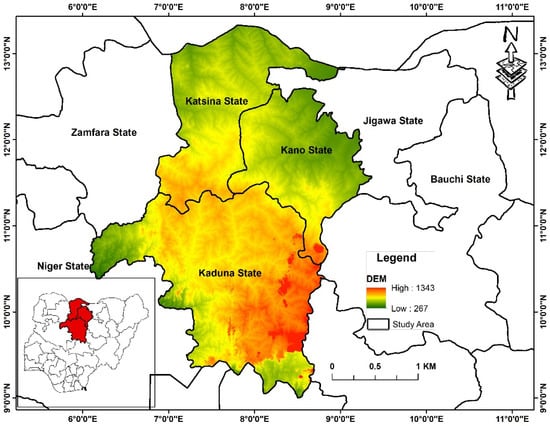
Figure 1.
Location Map of Nigeria’s Major Maize Producing States alongside their Digital Elevation Model (DEM).
2.2. Data and Pre-Processing
2.2.1. Sentinel-1 Satellite
Sentinel 1 satellites consist of two (2) polar-orbiting satellites. The first satellite was launched on 3 April 2014. A Europeanized Russian Soyuz rocket launched the second satellite on 25 April 2016. These two polar-orbiting satellites provide a reliable, broader geographical coverage, improved revisit, and rapid dissemination of information to support different operational usages in priority areas such as land monitoring and assessment, marine observation, and emergency services. The satellite’s dual polar-metric products help researchers and other users working on agriculture, land use/land cover classification, and forestry. The C-SAR instrument of the Sentinel 1-satellite supports processes in both horizontal and vertical polarization (i.e., HHþHV and VVþVH), which are implemented using one transmit chain (i.e., convertible to H or V) and two parallel receive chains for H and V polarization. The dual-polarization data of Sentinel 1 is useful for sea-ice applications and land use/land cover classification.
Sentinel-1 Ground Range Detected (GRD) C-band imagery (5.405 GHz) was accessed using Interferometry Wide Swath (IW). Using the IW mode, it is possible to cover a wide swath width (250 km) with a moderate geometric resolution (10 m). Level 1 processing of GRD products includes removing thermal noise, adjusting elevation antenna patterns, correcting range spreading loss, and using an Earth ellipsoid model to project data to the ground range. Images in each polarization (VH and/or W) are included in the GRD products. In the IW images, the pixel spacing is 10 m, and the azimuth incidence is 30° to 45°.
In this study, maize monitoring with microwave Sentinel-1A SAR data is carried out in three producing states in northern Nigeria during the growing seasons from 2016 to 2019.
IW mode Sentinel-IA GRD images employed in this study were accessed in the GEE platform from early January to December from 2016 to 2019 for temporal analysis. For mapping cropland and other land cover, the months of May to October were used; this time period encompassed the entire maize growing season from planting to the time of maize harvesting.
2.2.2. Sentinel-2 Satellite
Crop classification was conducted using the Sentinel-2 MSI remotely sensed satellite. As part of the Copernicus Programme, the European Space Agency (ESA) developed Sentinel-2 [8]. With its wide coverage (10 m to 60 m), fine spatial resolution, multispectral features (13 spectral bands), and frequent revisits (10 days with one satellite and 5 days with two satellites), the mission can track changes in vegetation during the growing season, monitor forests, find changes in land cover, and respond to natural disasters [17].
The Sentinel-2 mission aims to systematically monitor land surfaces and coastal areas by providing high-resolution optical imagery that offers comprehensive coverage and a high revisit period. In addition to its imaging capabilities, it provides a wealth of operational data products, including maps for change detection, bottom-of-atmosphere reflectance, and numerous geophysical variables, such as leaf chlorophyll content, leaf area index, and leaf water content.
Within its visible, near-infrared, and shortwave infrared spectral zones, Sentinel-2 has 13 spectral channels with a spatial resolution of 10–60 m. This helps in detecting spatiotemporal changes and vegetation state differences. Sentinel 2 satellites have 13 spectral bands, as shown in Table 1.

Table 1.
Sentinel-2 Bands.
2.2.3. Sample Data Acquisition
Global and regional crop mapping is crucial in developing countries, especially in sub-Saharan tropical regions where hunger and food insecurity are prevalent. As a result of this information, it is possible to evaluate, model, and quantify the productivity of maize crops.
Reference samples are essential to train and validate any supervised classification algorithm for maize mapping in three states (Kano, Kaduna, and Katsina). For the 2016–2019 growing seasons, we used official data from the International Institute of Tropical Agriculture (IITA) in Kano, Nigeria, covering the months of May to September each year. This field campaign’s primary objective was to increase small-scale African maize farmers’ crop production and financial success (Ethiopia, Tanzania, and Nigeria). The main target for this study is the maize crop; however, due to the spatial heterogeneity of the area, the presence of land cover classes might influence maize mapping results. For misclassification, broad land cover classes were listed.
In addition to maize fields, these broad classes include built-up areas, grasslands, bare lands, water bodies, and other types of terrain. Maize fields include all the maize plots observed. Build up comprises a housing and impervious surface, and grassland includes all the small plants grown in the study area. Bare soil comprises all of the uncultivated land. Water bodies include rivers, streams, lakes, or any stagnant water in the study area. Others may be described as any class that does not fall within the class categories mentioned above (forest, other vegetation, etc.). The final result could fall as others because of misclassification. The broad land-cover nomenclature was employed for all the years under study. This study adopted a random sampling method using predetermined regions and coordinates. The TAMASA program employs a rigorous scientific methodology to determine the optimal placement of plots based on various factors. These factors include the size, density, and structural variations of the sample region being studied. This approach ensures that the resulting data is reliable and representative of the larger population, enabling more accurate analyses and conclusions.
A substantial amount of training datasets and validation data sets of maize sample points were collected throughout the field campaigns for 2016, 2017, 2018, and 2019, using a Global Positioning System (GPS) device. These random points were recorded with reasonable accuracy from maize fields. Collecting field data is a resource-intensive and time-consuming activity covering large areas. The remaining five classes were delineated on-screen based on visually evaluating the geo-referenced Google Earth images and multi-spectral composites, and extra training and a validation sample were obtained at random in addition to the maize sample locations. We applied on-screen digitization for each sampling point to get a polygon to enclose each. These classes were gathered using Google Earth images under close supervision for visual assessment and local knowledge of the area. We identified six main Land Use/Land Cover classes within the study area according to the target crop (maize). Among them were maize fields, built-up areas, grasslands, bare lands, water bodies, and other classes. Figure 2 shows the training and validation samples for each year. Two-thirds of these sample data were used for training and one-third for validation for each class.
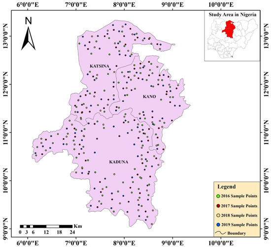
Figure 2.
Map of the Study Area showing the different Training and Validation Points.
3. Methodology
The framework illustrated in Figure 3 outlines the methodological workflow for the study’s seasonal crop inventory (SCI) mapping based on a machine-learning algorithm and Google Earth Engine.
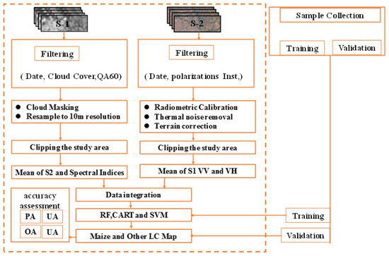
Figure 3.
Proposed Methodological Outline for the Mapping of Maize and Other Land Cover Categories.
3.1. Sentinel-1 Pre-Processing
IW modes associated with VV+VH polarisation over land are mainly conflict free. Hence, the GRD images obtained in IW mode with a spatial resolution of 10 m and ascending orbit were employed. Moreover, HH and HH/HV channels are deliberately intended for polar environments. Thus, they were uncommon in tropical areas such as Nigeria; therefore, VV and VH channels were employed.
As part of this study, Sentinel-1A images from (GRD) products within GEE were retrieved (Image Collection ID: COPERNICUS/S1_GRD). We utilized a cloud-based geospatial analysis platform known as GEE to process the products for analysis. This powerful tool enabled us to solve problems efficiently, making our processing more streamlined and effective. This system is ideal for processing and analysing earth observation data. The pre-processing of Sentinel-1A followed a chain that commenced with (a) applying orbit file to enhance geometric consistency in the image time series, (b) GRD border noise removal, (c) thermal noise removal in all images, (d) radiometric calibration to sigma nought (0°) backscatter coefficients (dB), and (e) terrain correction. The next step involved is then Boxcar filtering, and the subsequent VH and VV polarisation datasets were subset to the extent of the study area.
3.2. Sentinel-2 Pre-Processing
A cloud-based platform called Google Earth Engine (GEE) was used to pre-process Sentinel-2 images [2]. GEE is a common architecture for an open-access JavaScript Application Programming Interface (API). It provides cloud computing capability with a multi-petabyte catalogue of remote sensing data, allowing us to process gigantic volumes of data and achieve high results for all earth observation processing and analysis. A total of 188 scenes from Sentinel-2A and B were accessed from the GEE in 2016, 2017, 2018, and 2019, respectively.
In this study, all Sentinel-2 images of minimal cloud cover (<10%) obtained over Kaduna, Kano, and Katsina States of northern Nigeria from early May to October 2016 and 2019 are employed for mapping the maize area and yield. However, due to the frequency of clouds in this subtropical area, only composite images of Sentinel-2A and 2B were used as composite images in all the years under study (2016, 2017, 2018, and 2019), respectively.
One technique was considered for the extraction of spectral–temporal metrics with the belief that it tallies with the research goals. Generally, constructing the base dataset is crucial for any mapping or classification of crops. In this work, the S2 dataset’s composition begins in GEE, starting with a filtered and cloud-masked image collection and ending with final maps.
In this study, seasonal composite imagery was generated using the median reducer, a commonly used image-processing tool, to produce cloud-free composites. The study selected satellite images from three northern Nigerian states based on the region of interest and focused on the summer season, specifically from May to October.
- (i)
- Sentinel-2 Data Fetching: Sentinel-2A and 2B of Multi-spectral Imaging (MSI) format are utilized in this study. These were dense time-series Sentinel-2A and 2B data span from May to October of the study years under investigation (2016, 2017, 2018, and 2019) with 5 or 10 day intervals.
- (ii)
- The GEE processing interface was utilized to retrieve the Sentinel-2 scenes needed for this research directly from the GEE image collection, negating the necessity of downloading the data to a local computer. This image collection comprises Sentinel-2 scenes.
- (iii)
- Cloud Filtering: In this study, GEE’s image collection contains different information about Sentinel-1 and 2 images. This includes acquisition mode, resolution, and pass type, etc. Thus, the selected images are suitable per user criteria known as “cloud filtering.” Using Metadata and Filtering, followed by a spatial subset, the study area is determined in GEE. The images used for this study were all selected from the orbit container of Sentinel-2 in the GEE. Later, the historical data are arranged using the filterdate argument.
- (iv)
- Cloud masking (maskS2clouds): The cloud cover for Sentinel-2 (S2) data is typically determined through computation of the QA60 band in conjunction with S2 surface reflectance data, both of which are available in Google Earth Engine (GEE). The QA60 layer, with a 60-m resolution, includes dense and cirrus clouds.
- (v)
- Composition creation: The chosen process created in this study, one image collection, including 188 images of the S2 with the “inBands”. In this study, we computed the median bands using the Google Earth Engine (GEE) platform. Additionally, we extracted several commonly used vegetation indices, namely, the Normalized Difference Vegetation Index (NDVI), Bare Soil Index (BSI), Modified Normalized Difference Water Index (MNDWI), Red Edge Position (REP), Modified Chlorophyll Absorption Reflectance Index (MCARI), Weighted Difference Vegetation Index (WDVI), Soil-Adjusted Vegetation Index (SAVI), Structure Intensive Woody Savanna Index (SIWSI), and the Enhanced Vegetation Index (EVI), for each image. The statistical analysis of relative spectral indices is carried out by applying Equations (1)–(8).
- (vi)
- Export to Asset: This is the final exporting stage with regard only to the desired bands, also known as (“outBands”), as previously stated. In this application, bands 2, 3, 4, 6, 8, 8A, 11, and 12 were chosen to construct the first S2 dataset.
To generate the final composite image of the study area, it is necessary to compute the median pixel values for each selected band and the composite images. Finally, we then export the bands of the dataset and the composite images to the asset within the GEE.
MNDWI = (Green − SWIR)/(Green + SWIR),
3.3. Feature Extraction
Sometimes, multi-spectral satellite images such as optical (Sentinel-2) and microwave (Sentinel-1) derived ones are often of a high correlation, similarity, and repetition [9]. As a result of the “curse of dimensionality” or the “Hughes effect,” there is an increase in positive correlations between adjacent bands [18]. An increase in the number of bands in an image would result in a tenfold increase in the number of observations required to train a classifier. Prior to performing the classification, the most significant or most useful feature (S1 and S2) datasets were chosen. As a result, data redundancy and correlation would be reduced.
In order to select optimal features for classification, we used the Gini index derived from the RF [12]. In ensemble machine learning, multiple trees are combined. In a test classification, two-thirds of the training records are applied for constructing the trees, and the remaining records are used for an “out-of-bag error”. The Gini impurity criterion for descendent nodes for RF training is less than that for the parent node whenever a split is conducted on a variable. Overall, trees are in the classification forest, and the importance score represents the sum of each variable’s Gini decreases. We used the RF method to calculate Gini importance scores in GEE.
3.4. Maize and Other Land Cover Classification
3.4.1. Random Forest (RF)
RF is an ensemble classifier, using a vast number of single decision trees to overcome single decision tree weaknesses [13,19]. Each unknown is assigned a final class based on the majority “vote” of all trees. Rather than relying solely on one tree to achieve optimum results, this approach incorporates a number of trees to achieve a global optimum. By incorporating many trees, a global optimum should be attained, thereby overcoming the problem that any one tree may have caused. The concept is further expanded by generating a random subset of training data for each tree; an element of this tree is selected based on a subset of its variables. A large amount of data can be classified efficiently with this classifier while handling imbalanced input features [20]. In RF classification, two main parameters are needed: the number of classification trees and the number of input features to use. Using the tune function, we determined the optimal parameter randomly. In this study, we determined the optimal number of trees to be 100, while the ideal number of datasets (mtry) was established as the square root of the total number of datasets. One of the strengths of RF is its ability to detect valuable information in each feature. In terms of efficiency and accuracy, RF classifiers possess the best results. One of its disadvantages is that many trees render trees ineffective at being visualized [21]. The classification was performed using the RF classifier from GEE [2].
3.4.2. Support Vector Machine (SVM)
The Support Vector Machine (SVM) is a powerful machine learning algorithm that has been successfully employed in the classification of remote sensing images [22,23,24]. Support vector machines have gained significant popularity in remote sensing applications for crop mapping, primarily due to their high success rate in classification [25]. An SVM is a method for non-parametric statistical learning [23]. SVM utilizes various types of kernels to transform nonlinear boundaries into linear ones, thereby enabling the determination of optimal hyperplanes in high-dimensional space. This approach has proven highly effective, allowing SVM to achieve remarkable accuracy in classifying complex datasets. [23,26]. As an integral component of its strategy, Support Vector Machine (SVM) obtains an optimal hyperplane from the training data of two or more classes within the feature space. This is achieved by maximizing the margins between the hyperplane and the closest training samples, enabling data classification with remarkable accuracy [27]. Radial basis function kernels are generally easier to define and give good results relative to other kernels when mapping crop types and land-use/cover mapping [28,29]. SVM classification accuracy is heavily dependent on the penalty parameter (C). Further, an SVM model uses a high value of C results in a more accurate prediction. Thus, we select a high value of 100. Conversely, the value of the gamma parameter was established as the inverse of the number of spectral bands. It plays a crucial role in the SVM algorithm, as it determines the degree of influence each training example has on the decision boundary. This study employed an open-source and free GEE platform to handle raster images.
3.4.3. Classification and Regression Tree (CART)
In 1984, Breiman et al. [21] proposed classification and regression trees (CARTs) [30]. CART is an algorism that can be employed for both classification and variable predictions. It is similar to RF. This approach uses supervised machine learning and employs training samples to construct trees in order to solve the classification problem. In other words, the CART algorithm divides data into subsets at each tree node based on the normalized information gain, which is the defining attribute of the split. A final decision is then made based on the attribute with the highest normalized information value. As a result, CART is often used to classify remote sensing data. A minimum number of leaves and a maximum number of nodes are set in GEE.
3.5. Accuracy Assessment
In order to accept a classification result, it is crucial to evaluate the accuracy of the result [31]. As a general rule, accuracy is measured by the degree of agreement between the results and the values assumed to be true [32]. Confusion matrices were applied to determine the overall accuracy (OA), producer accuracy (PA), and user accuracy (UA) of crop and land cover maps [31]. The overall accuracy is generally based on the number of correctly classified reference pixels compared to the number of correctly classified pixels. As Congalton and Green [33] state, analysing the confusion matrix to determine the causes of differences can be a very relevant and fascinating step in constructing a remote sensing map. Maize and other LC classifications are evaluated using a confusion matrix built into GEE. Using this matrix, the output classification is compared statistically with the maize and other LC associated with the validation points. The error matrix was computed using Equation (9).
3.6. F-Score
F-Score is employed to evaluate classified maps. A statistic measuring accuracy based on the confusion matrices (accuracy assessment statistics) for each class has been calculated using Equation (10). The F1-score is computed as the harmonic mean of precision and recall, which are two fundamental metrics used to measure both producer and user accuracy. It is an essential indicator for evaluating classification models compared with independent producer and user indicators [34]. In terms of accuracy, both producers and users have their own shortcomings. A high threshold will result in high producer accuracy, but there will be a lot of data loss; a low threshold will result in high user accuracy but inaccurate predictions. In this way, the F1-score allows a more comprehensive classifier evaluation while simultaneously allowing for producers and users to be balanced. The F1-score was computed using Equation (10).
In this case, PA represents the accuracy of the producer, and UA represents the accuracy of the user.
4. Results
4.1. Integration of Selected Sentinel-1 and 2 Data for Spatial Mapping of Maize Distribution
The spatial distribution of maize maps in three major maize-producing states in 2016, 2017, 2018, and 2019 derived from selected optical and SAR data using Random Forest (RF) are presented in Figure 4. It can be seen in Figure 4 that the maize spatial distribution is not similar between the selected sentinel-1A and 2A data across years, with more maize pixels being observed in 2017, 2018, and 2019. With the optimum data, there was a higher amount of maize in 2017, 2018, and 2019.
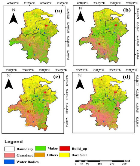
Figure 4.
Spatial Mapping of Maize and other Land Cover Types in Kano, Katsina, and Kaduna State derived from Sentinel-1 and 2 Data using (a) RF in 2016, (b) RF in 2017, (c) RF in 2018, and (d) RF in 2019.
Figure 4 shows pixel-based maize and other land cover maps for 2016–2019. Using the cloud-computing platform GEE, the RF algorithm and selected Sentinel 1 and 2 imagery features were used to produce these maps. The proposed method successfully classified maize cropland and other land cover classes through visual interpretation. The pixel-based accuracies of the selected feature of Sentinel-1 and -2 imagery are presented in Table 2.
Table 2.
The Confusion Matrix showing the Producer’s Accuracy (PA), User’s Accuracy (UA), Overall Accuracy (OA), and Cohen’s K (KC) of the Maize Crop and other Land Cover produced using the Random Forest method for 2016–2019.
We produced maize and other land cover maps for 2016–2019 with a 10 m resolution based on Sentinel-2 and Sentinel-1 satellites in the Cloud computing platform provided by GEE. Figure 5 displays two subsets of maps depicting maize and other land covers. It appears that most of the maize pixels have been correctly classified based on the classified result (Figure 5a,b). Because of the post-processing to reduce noise (salt and pepper), the resulting RCI maps are visually clear and noise-free. With the help of visual interpretation, maize and other classes could be detected and classified reasonably well using the proposed method. In the first zoomed region (Figure 5a), most people engage in farming activities in the northern part of Katsina state (Bakori). According to the proposed approach, maize crops and other land cover types could be identified successfully. Furthermore, the proposed method could identify several fragmented maize crops in this region. In addition, the proposed method effectively classified maize and other land cover classes in Makarfi, located in the southern part of Kaduna state (Figure 5b). There are several maize fields in this region, where a large amount of maize is produced yearly. Our study shows that the proposed GEE workflow effectively classifies maize crops and other land covers in three states (Kano, Kaduna, and Katsina). Nevertheless, there were differences in the boundaries between maize crop pixels and other land cover classes. For example, some low microwave backscatter in the mixed pixels may be from grasslands, others, and bare soil. Other classification algorithms, such as CART and SVM, were also compared with RF.
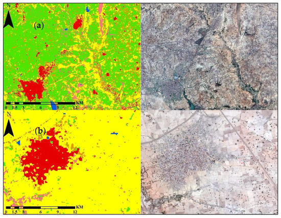
Figure 5.
Depicts the Seasonal Crop Inventory (SCI) Map and other land cover classes for the year 2016, specifically focusing on two regions, namely, Bakori and Makarfi, as illustrated in (a,b), respectively. Accompanying these maps are high-resolution satellite images that were employed for visual assessment purposes.
In the map produced in 2016, PA, and UA were, respectively, 0.99 % and 0.99%. This indicates that cloud computing has great potential for SCI production. In contrast, the PA and UA values of the other land cover classes ranged from 0.93% to 0.98%. In terms of PA and UA, the built-up class ranked highest after the maize crop class. The OA and KC were, respectively, 0.97% and 0.97%. As you can see from Table 2, the classification performance of maize and the remaining classes in the different periods also shows excellent results in terms of UA and PA. For the classified classes in 2017, 2018, and 2019, a high OA of 0.98%, 0.97%, and 98% was achieved. On the other hand, the UA for other land cover classes was either equal or higher than the PA. It is clear from the results that these maize maps and other land cover classes may satisfactorily reflect some of the dynamics of the maize crop in the study area during the past four years. A relatively good F-score was obtained from the selected Sentinel 1 and Sentinel 2 data. During the past four years, discriminative capabilities for maize and remaining land cover classes (>0.90) have been demonstrated.
4.2. VV and VH Annual Profiles
Utilizing different VH and VV polarizations and accounting for varying growth stages of maize plants and other land cover classes, we have conducted an in-depth analysis of the temporal and seasonal changes in Sentinel-1 backscatter. The S-1 seasonal time series for VV and VH polarization in ascending orbits are presented in Figure 6 and Figure 7, respectively. The original S-1 data has been processed and filtered to produce accurate results. Our estimates reveal that the coefficient of backscattering σ0 in maize VH polarization ranges from [−20.12 to −18.95] dB, whereas the build-up class exhibits a range of [−14.29 to −15.29] dB. Conversely, water has a backscattering coefficient range of [−23.12 to −21.95] dB. Furthermore, grassland has a backscattering coefficient ranging from [−17.31 to 17.73] dB. The bare soil and other land cover classes are estimated to fall within the range of [−14.29 to −15.29] and [−19.75 to −19.95] dB, respectively, over the years under investigation. In terms of VV polarization, our findings suggest that maize exhibits a range of [−10.65 to −10.86] dB, while build-up has a range of [−5.57 to −5.87] dB. The coefficient of backscattering for water is approximately −15.23 to −15.47 dB, while grassland falls within the range of [−11.01 to −11.33] dB. Bare soil is estimated to be around [−12.06 to −12.49] dB, and others are approximately [−10.29 to −10.62] dB.
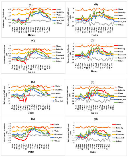
Figure 6.
Backscatter Coefficient Curves for Maize and other Land Cover Types derived from Sentinel-1 Images (VH and VV) during 2016 (A,B), 2017 (C,D),2018 (E,F) and 2019 (G,H) Growing Seasons.
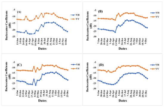
Figure 7.
Backscatter Coefficient Curves of Maize derived using Sentinel-1 Images of VH and VV Polarizations from 2016 (A), 2017 (B), 2018 (C) and 2019 (D).
To investigate the backscattering characteristics of maize and other land cover categories, we analyzed Figure 6 and Figure 7. Our findings revealed that the S-1A VH and VV time series exhibited seasonal trends consistent with the patterns observed in maize crops and other land cover types throughout the study area’s growing season. Given the nature of water, it was observed that VV and VH values were the lowest among all categories in all years due to absorption and mirror reflection towards the radar antenna. Conversely, the build-up class exhibited the highest backscattering coefficient values. Moreover, the bare soil category displayed the lowest VV and VH image values compared to the remaining class types after water. Finally, grassland cover types exhibited the highest backscattering coefficient values after build-up.
The analysis of maize using radar backscattering coefficients revealed distinct temporal and seasonal trends for sigma VV and VH, with VH exhibiting a more pronounced response to maize growth than sigma VV (as shown in Figure 7A–D). Based on these findings, we identified four distinct growth stages of maize. The first stage, characterized by low VH and VV backscattering coefficients, occurs when the land is clear. The second stage is marked by a gradual and rapid transition associated with maize growth, during which both VH and VV increase faster than other land cover classes (excluding built-up areas). The third stage is the main growing season in summer, during which VH and VV values plateau. This period coincides with the anthesis-silking stage when the maize stem leaves become wider than any other plants in the surrounding area. In the fourth and final stage, VH and VV values decrease, corresponding with the time of leaf senescence. Notably, both polarizations increased during tillering, followed by a stabilization period before decreasing to ripening after fluorescence.
5. Discussion
In recent years, the field of remote sensing (RS) has experienced exponential growth due to advancements such as new satellites, increased sensor resolutions, and the availability of massive free data archives. Furthermore, the increased computational power of computers has made it possible to process and analyze large amounts of data quickly. Google Earth Engine (GEE) is a free, open-source platform that has been highly successful as a geospatial analysis and modeling tool thanks to its vast archive of ready-to-use data. GEE allows users to easily access, analyze, and visualize geospatial data. This study demonstrates how combining GEE, machine learning (ML) algorithms, and geographical pixel-based analysis can create multi-temporal composite images for streamlined crop classification processes. The results show that this approach can be highly effective, providing an efficient and straightforward way to process complex image data.
In this research paper, a user-friendly, freely accessible GEE code was developed that integrated microwave data derived from Sentinel-1, optical data derived from Sentinel-2, and machine learning (ML) algorithms. The code allows users to set and adjust various input parameters and compare results obtained from different classification approaches, such as Random Forest (RF), classification and regression trees (CART), and support vector machines (SVM). The same input dataset and classification algorithm are used, making it easy to visually compare the output maps of maize and other land covers. The accuracy matrix of a given study area can also be analysed to determine the effectiveness of the classification approach. The results of this study confirm previous findings [20] that the RF algorithm provides higher accuracy than CART and SVM algorithms in most cases. This integration of microwave and optical data with ML algorithms in a user-friendly GEE code represents a significant advancement in the field of remote sensing, providing researchers with a powerful tool for analysing and classifying land cover data. RF is not always the best option for accuracy. Studies have shown that, in some cases, other algorithms may perform better than RF, especially when dealing with imbalanced datasets. In addition, algorithms depend on the size and complexity of the data, the computational resources available, and the specific goals of the analysis. Despite the benefits of RF for many situations, it cannot be considered a one-size-fits-all classification solution. Researchers and practitioners should carefully consider its strengths and limitations before selecting a machine learning algorithm that best fits their needs and objectives [35].
The accuracy of classification models depends heavily on the number and quality of the training points and the validation points used. As a result of the significant challenges that the study areas have faced in recent years, it has been challenging to collect reliable and comprehensive data from these areas due to the lack of resources available. The challenges include insecurity in the form of armed highway robbery, cattle rustling, kidnapping for ransom, and raiding villages, which have caused extensive damage to families and communities. Furthermore, these challenges have deepened mistrust along the traditional fault lines of ethnic and religious differences, making it challenging to collect data from some areas. Despite these challenges, there is an opportunity to use the computational potential of Google Earth Engine (GEE) to quickly acquire training points and validation points without physically traveling to all regions. This approach could pave the way for the possibility of exploiting the vast amounts of data available through GEE to train and validate classification models accurately. The advantage of this method is that it enables researchers to access up-to-date, high-resolution satellite imagery and process large amounts of data quickly and accurately. This approach could be advantageous in regions where security challenges make physical data collection difficult or impossible.
There is a similarity in spectral properties between maize and other crops. Based on our study, we identified six classes, but some of them had similar physical and spectral characteristics, making it difficult to distinguish them. Our analysis of the classes was based on the use of spectral and SAR features over multiple periods (from 2016 to 2018). The results showed a significant overlap between the pixel values of maize and other croplands, which led to difficulties in accurately classifying these classes. It was observed that there was considerable confusion between some of the classes, which was in agreement with the confusion matrix (Table 2) as well as the final SCI map (Figure 7). Furthermore, a few misclassifications were observed, which is a strong indication that further developments could be made to the classification algorithm. The study highlights the importance of combining different types of data, such as optical and SAR imagery, to overcome the limitations of individual data sources and improve the accuracy of land cover classification.
6. Conclusions
The primary objective of this study was to create a comprehensive classification and mapping maize cropland and other land cover classes in the northern region of Nigeria. The research serves as a pioneer study in Nigeria that examined the potential of the Google Earth Engine platform and machine learning techniques using satellite imagery such as Sentinel 1 and Sentinel 2 in the maize-producing states of northern Nigeria in 2016–2019. We applied GEE to identify maize cropland and other land cover classes in three Nigerian states using different classification algorithms, including Random Forest (RF), Support Vector Machine (SVM), and Classification Regression Trees (CART). The study indicated a comprehensive classification of heterogeneous smallholder fields in the study areas of Kaduna, Kano, and Katsina states. Therefore, the present study demonstrated the versatility and reliability of using Google Earth Engine (GEE) for cropland mapping. To validate the results, the average overall accuracy for 2016–2019 was 97%, and the average producer and user accuracy for maize crop classes were approximately 98% and 93%, respectively. This level of accuracy is above satisfactory and is reliable for pioneer research that utilizes GEE to create a Seasonal Crop Inventory (SCI). The method employed is a technological advancement that is cost-effective and efficient. The utilization of the proposed method and the study’s findings could have significant implications for Nigerian Cropland Inventories (NCI) development and for the detection and monitoring of changes, as demonstrated in this study. Therefore, for future research, a more accurate and reliable SCI map can be produced by considering that despite attaining a high level of overall accuracy, collecting additional field data is necessary to accurately map other crop categories. Therefore, future studies could improve the class accuracy with a better algorithm for mapping various crops in non-cropland areas. The Seasonal Crop Inventory maps of other regions in Nigeria could also be produced. In addition, future studies classifying cropland could utilize high-resolution satellite images such as Quick Bird, GeoEye, and WorldView for improved classification accuracy.
Author Contributions
Conceptualization, G.A.A. and K.W.; methodology, G.A.A.; software, A.F.K.; validation, G.A.A., K.W. and A.F.K.; formal analysis, G.A.A.; investigation, K.W.; resources; writing—original draft preparation, G.A.A.; writing—review and editing, A.F.K., M.I.H. and K.A.M.S.; visualization, K.A.M.S.; supervision, K.W.; project administration, K.W. and M.G.; funding acquisition, K.W. and J.D. All authors have read and agreed to the published version of the manuscript.
Funding
This research was funded jointly by the National Natural Science Foundation of China, grant No. 41971236 and the National Key Research and Development Program of China, grant number 2020YFC1807500.
Data Availability Statement
The data presented in this research article are available from the corresponding author on request.
Conflicts of Interest
The authors declare no conflict of interest.
References
- Abubakar, G.A.; Wang, K.; Shahtahamssebi, A.; Xue, X.; Belete, M.; Gudo, A.J.A.; Shuka, K.A.M.; Gan, M. Mapping Maize Fields by Using Multi-Temporal Sentinel-1A and Sentinel-2A Images in Makarfi, Northern Nigeria, Africa. Sustainability 2020, 12, 2539. [Google Scholar] [CrossRef]
- Gorelick, N.; Hancher, M.; Dixon, M.; Ilyushchenko, S.; Thau, D.; Moore, R. Google Earth Engine: Planetary-Scale Geospatial Analysis for Everyone. Remote Sens. Environ. 2017, 202, 18–27. [Google Scholar] [CrossRef]
- Amani, M.; Ghorbanian, A.; Ahmadi, S.A.; Kakooei, M.; Moghimi, A.; Mirmazloumi, S.M.; Moghaddam, S.H.A.; Mahdavi, S.; Ghahremanloo, M.; Parsian, S.; et al. Google Earth Engine Cloud Computing Platform for Remote Sensing Big Data Applications: A Comprehensive Review. IEEE J. Sel. Top. Appl. Earth Obs. Remote Sens. 2020, 13, 5326–5350. [Google Scholar] [CrossRef]
- Tamiminia, H.; Salehi, B.; Mahdianpari, M.; Quackenbush, L.; Adeli, S.; Brisco, B. Google Earth Engine for Geo-Big Data Applications: A Meta-Analysis and Systematic Review. ISPRS J. Photogramm. Remote Sens. 2020, 164, 152–170. [Google Scholar] [CrossRef]
- Xiong, J.; Thenkabail, P.S.; Gumma, M.K.; Teluguntla, P.; Poehnelt, J.; Congalton, R.G.; Yadav, K.; Thau, D. Automated Cropland Mapping of Continental Africa Using Google Earth Engine Cloud Computing. ISPRS J. Photogramm. Remote Sens. 2017, 126, 225–244. [Google Scholar] [CrossRef]
- Li, Q.; Qiu, C.; Ma, L.; Schmitt, M.; Zhu, X.X. Mapping the Land Cover of Africa at 10 m Resolution from Multi-Source Remote Sensing Data with Google Earth Engine. Remote Sens. 2020, 12, 602. [Google Scholar] [CrossRef]
- Kumar, L.; Mutanga, O. Google Earth Engine Applications since Inception: Usage, Trends, and Potential. Remote Sens. 2018, 10, 1509. [Google Scholar] [CrossRef]
- Drusch, M.; Del Bello, U.; Carlier, S.; Colin, O.; Fernandez, V.; Gascon, F.; Hoersch, B.; Isola, C.; Laberinti, P.; Martimort, P.; et al. Sentinel-2: ESA’s Optical High-Resolution Mission for GMES Operational Services. Remote Sens. Environ. 2012, 120, 25–36. [Google Scholar] [CrossRef]
- Pacifici, F.; Chini, M.; Emery, W.J. A Neural Network Approach Using Multi-Scale Textural Metrics from Very High-Resolution Panchromatic Imagery for Urban Land-Use Classification. Remote Sens. Environ. 2009, 113, 1276–1292. [Google Scholar] [CrossRef]
- World Bank. Data Report on Agricultural Land. 2020. Available online: https://data.worldbank.org/indicator/AG.LND.AGRI.K2?locations=NG (accessed on 25 April 2023).
- Okou, C.; Spray, J.; Unsal, D.F. Africa Food Prices Are Soaring Amid High Import Reliance. Available online: https://www.imf.org/en/Blogs/Articles/2022/09/26/africa-food-prices-are-soaring-amid-high-import-reliance (accessed on 22 February 2022).
- Strobl, C.; Boulesteix, A.L.; Zeileis, A.; Hothorn, T. Bias in Random Forest Variable Importance Measures: Illustrations, Sources and a Solution. BMC Bioinform. 2007, 8, 25. [Google Scholar] [CrossRef]
- He, Y.; Lee, E.; Warner, T.A. A Time Series of Annual Land Use and Land Cover Maps of China from 1982 to 2013 Generated Using AVHRR GIMMS NDVI3g Data. Remote Sens. Environ. 2017, 199, 201–217. [Google Scholar] [CrossRef]
- Abubakar, G.A.; Wang, K.; Belete, M.; Shahtahamassebi, A.R.; Biswas, A.; Gan, M. Toward Digital Agricultural Mapping in Africa: Evidence of Northern Nigeria. Arab. J. Geosci. 2021, 14, 643. [Google Scholar] [CrossRef]
- Bank, W. Poverty Reduction in Nigeria in the Last Decade; World Bank: Washington, DC, USA, 2016. [Google Scholar]
- Otekunrin, O.A.; Otekunrin, O.A.; Momoh, S.; Ayinde, I.A. How Far Has Africa Gone in Achieving the Zero Hunger Target? Evidence from Nigeria. Glob. Food Sec. 2019, 22, 1–12. [Google Scholar] [CrossRef]
- Vuolo, F.; Zóltak, M.; Pipitone, C.; Zappa, L.; Wenng, H.; Immitzer, M.; Weiss, M.; Baret, F.; Atzberger, C. Data Service Platform for Sentinel-2 Surface Reflectance and Value-Added Products: System Use and Examples. Remote Sens. 2016, 8, 938. [Google Scholar] [CrossRef]
- Bellman, R. Dynamic Programming, 2nd ed.; Dover Publications: Mineola, NY, USA, 2003. [Google Scholar]
- Cutler, D.R.; Edwards, T.C.; Beard, K.H.; Cutler, A.; Hess, K.T.; Gibson, J.; Lawler, J.J. Random Forests for Classification in Ecology. Ecology 2007, 88, 2783–2792. [Google Scholar] [CrossRef]
- Rodriguez-Galiano, V.F.; Ghimire, B.; Rogan, J.; Chica-Olmo, M.; Rigol-Sanchez, J.P. An Assessment of the Effectiveness of a Random Forest Classifier for Land-Cover Classification. ISPRS J. Photogramm. Remote Sens. 2012, 67, 93–104. [Google Scholar] [CrossRef]
- Breiman, L. Random Forests. Mach. Learn. 2001, 45, 5–32. [Google Scholar] [CrossRef]
- Mountrakis, G.; Im, J.; Ogole, C. Support Vector Machines in Remote Sensing: A Review. ISPRS J. Photogramm. Remote Sens. 2011, 66, 247–259. [Google Scholar] [CrossRef]
- Pal, M.; Mather, P.M. Support Vector Machines for Classification in Remote Sensing. Int. J. Remote Sens. 2005, 26, 1007–1011. [Google Scholar] [CrossRef]
- Huang, C.; Davis, L.S.; Townshend, J.R.G. An Assessment of Support Vector Machines for Land Cover Classification. Int. J. Remote Sens. 2002, 23, 725–749. [Google Scholar] [CrossRef]
- Moumni, A.; Lahrouni, A. Machine Learning-Based Classification for Crop-Type Mapping Using the Fusion of High-Resolution Satellite Imagery in a Semiarid Area. Scientifica 2021, 2021, 8810279. [Google Scholar] [CrossRef]
- Mathur, A.; Foody, G.M. Crop Classification by Support Vector Machine with Intelligently Selected Training Data for an Operational Application. Int. J. Remote Sens. 2008, 29, 2227–2240. [Google Scholar] [CrossRef]
- Gholami, R.; Fakhari, N. Chapter 27—Support Vector Machine: Principles, Parameters, and Applications. In Handbook of Neural Computation; Samui, P., Sekhar, S., Balas, V.E., Eds.; Academic Press: New York, NY, USA, 2017; pp. 515–535. [Google Scholar] [CrossRef]
- Löw, F.; Knöfel, P.; Conrad, C. Analysis of Uncertainty in Multi-Temporal Object-Based Classification. ISPRS J. Photogramm. Remote Sens. 2015, 105, 91–106. [Google Scholar] [CrossRef]
- Petropoulos, G.P.; Kalaitzidis, C.; Prasad Vadrevu, K. Support Vector Machines and Object-Based Classification for Obtaining Land-Use/Cover Cartography from Hyperion Hyperspectral Imagery. Comput. Geosci. 2012, 41, 99–107. [Google Scholar] [CrossRef]
- Tucker, C.J. Red and Photographic Infrared Linear Combinations for Monitoring Vegetation. Remote Sens. Environ. 1979, 8, 127–150. [Google Scholar] [CrossRef]
- Koko, A.F.; Wu, Y.; Abubakar, G.A.; Alabsi, A.A.N.; Hamed, R.; Bello, M. Thirty Years of Land Use/Land Cover Changes and Their Impact on Urban Climate: A Study of Kano Metropolis, Nigeria. Land 2021, 10, 1106. [Google Scholar] [CrossRef]
- Tassi, A.; Vizzari, M. Object-Oriented LULC Classification in Google Earth Engine Combining SNIC, GLCM, and Machine Learning Algorithms. Remote Sens. 2020, 12, 3776. [Google Scholar] [CrossRef]
- Congalton, R.G.; Green, K. Assessing the Accuracy of Remotely Sensed Data: Principles and Practices; CRC Press: Boca Raton, FL, USA, 2009; Volume 2, ISBN 0873719867. [Google Scholar]
- Chicco, D.; Jurman, G. The Advantages of the Matthews Correlation Coefficient (MCC) over F1 Score and Accuracy in Binary Classification Evaluation. BMC Genom. 2020, 21, 6. [Google Scholar] [CrossRef]
- Xie, Q.; Wang, J.; Liao, C.; Shang, J.; Lopez-Sanchez, J.M.; Fu, H.; Liu, X. On the Use of Neumann Decomposition for Crop Classification Using Multi-Temporal RADARSAt-2 Polarimetric SAR Data. Remote Sens. 2019, 11, 776. [Google Scholar] [CrossRef]
Disclaimer/Publisher’s Note: The statements, opinions and data contained in all publications are solely those of the individual author(s) and contributor(s) and not of MDPI and/or the editor(s). MDPI and/or the editor(s) disclaim responsibility for any injury to people or property resulting from any ideas, methods, instructions or products referred to in the content. |
© 2023 by the authors. Licensee MDPI, Basel, Switzerland. This article is an open access article distributed under the terms and conditions of the Creative Commons Attribution (CC BY) license (https://creativecommons.org/licenses/by/4.0/).