MV-CDN: Multi-Visual Collaborative Deep Network for Change Detection of Double-Temporal Hyperspectral Images

Abstract

Since individual neural networks have limited deep expressiveness and effectiveness, many learning frameworks face difficulties in the availability and balance of sample selection. As a result, in change detection, it is difficult to upgrade the hit rate of a high-performance model on both positive and negative pixels. Therefore, supposing that the sacrificed components coincide perfectly with the important evaluation objectives, such as positives, it would lose more than gain. To address this issue, in this paper, we propose a multi-visual collaborative deep network (MV-CDN) served by three collaborative network members that consists of three subdivision approaches, the CDN with one collaborator (CDN-C), CDN with two collaborators (CDN-2C), and CDN with three collaborators (CDN-3C). The purpose of the collaborator is to re-evaluate the feature elements in the network transmission, and thus to translate the group-thinking into a more robust field of vision. We use three sets of public double-temporal hyperspectral images taken by the AVIRIS and HYPERION sensors to show the feasibility of the proposed schema. The comparison results have confirmed that our proposed schema outperforms the existing state-of-the-art algorithms on the three tested datasets, which demonstrates the broad adaptability and progressiveness of the proposal.

1. Introduction

Change detection of hyperspectral images is a hot application in remote sensing. To detect the earth surface changes resulting from natural causes or human activities in the same geographic location over time, double-temporal images, which contain a former image captured at a certain time and a detected image acquired at a later point in time, are needed. This technique is highly applied in many fields, e.g., eco-environmental protection [1,2], urban sprawl [3,4], land application [5,6], farmland changes [7,8], geological disaster monitoring [9,10], as well as forest and wetland conservation [11]. With the development of multitemporal real-time monitoring, intelligent scene surveillance [12,13,14] and warning forecast systems were pushed to fresh highs.

In the remote-sensing field, although multispectral images [6] and synthetic aperture radar (SAR) images [15] demonstrate good performance in the domain of change detection, they show some weaknesses in terms of limited spectral information. It is fortunate that hyperspectral images (HSIs) can carry more detailed descriptions about real physical objects because of the wider spectrum. This favors the performance improving of change detection, e.g., through the novel method using multiple morphological profiles (MMPs) proposed by Hou et al. [16]. To fully utilize the important spectral and temporal sequences of HSIs, Wang et al. [17] proposed to join the spectral, spatial, and temporal for change detection on HSIs. However, the important spectral and temporal sequences for HSIs are easily ignored. As shown in a literature survey, though many HSIs-oriented change-detection methods have been developed, this does not mean they can satisfactorily solve the difficulties caused by the inevitable and unexpected change factors occurring in the specific wave domains [18]. The traditional practice is to first reduce the dimensional structure or determine the hoped-for bands selected from hundreds of bands for efficient analysis. However, although it is beneficial in removing noise and improving computational efficiency, high-dimensionality reduction may cause the loss of effective features, which will lead to a matter of mistaken identity.

To minimize the above problems and reduce the misidentification rate, some researchers proposed to make use of all spectral bands for the sake of maximizing the amount of information and improving the detection performance. In this respect, deep neural networks (DNNs) possess arbitrary nonlinear expressiveness [19] and are regarded as the main content of studies. On the premise of full-band information, the breakthrough points of the DNN-based methods usually include supervised algorithms [20,21], feature enhancement [22,23], ways to avoid negative factors, optimization of objective loss function [24] for applicability requirements, etc. With the efforts of many researchers, extraordinary progress has been made in these respects. However, the deep expressiveness of a DNN model is limited, and we found no cases about translating the group-thinking of collaborative network members resulting from the fine-tuning of a prototypical model into a more robust field of vision.

Accordingly, we propose to employ three light-weight collaborative network members with sensitivity disparity to serve the multi-visual collaborative deep network (MV-CDN). In fact, each collaborative network member can independently generate the projection features for change-detection analysis, the corresponding network architecture, transformation process, and the theory of loss function are detailed in Section 3. As collaborative network members, the fully connected network (FCNet) is applied in the state-of-the-art model deep slow feature analysis (DSFA) [25]. With SFA, it demonstrates the effectiveness and practicality for change detection in hyperspectral images; the sensitivity disparity networks (SDN) [26], which consist of an unchanged sensitivity network (USNet) we have proposed in our previous work [27] and is also known as dual-path partial recurrent networks (D-PRNs); and a changed sensitivity network (CSNet). The special note is that the SDN members, USNet and CSNet, result from the fine-tuning of FCNet and extensive testing has proven that they are more sensitive to unchanged pixels and more sensitive to changed pixels, respectively. The collaborators are selectively applied to the network layers of collaborative network members to translate the group-thinking of collaborative network members into a more robust field of vision and thus to construct the three branch approaches: CDN with one collaborator (CDN-C) on the output layer (OL), CDN with two collaborators (CDN-2C) on the output layer and the second hidden layer (HL-2), and CDN with three collaborators (CDN-3C) on the output layer, the HL-2 and the first hidden layer (HL-1), respectively.

Table 1. The relationship among learning collaborator (LC), output collaborator (OC), the first hidden layer (HL-1), the second hidden layer (HL-2), the output layer (OL), in three subdivision approaches: CDN with one collaborator (CDN-C), CDN with two collaborators (CDN-2C), CDN with three collaborators (CDN-3C). The “×” means not available.

Collaborator	CDN-C	CDN-2C	CDN-3C
HL-1	×	×	LC
HL-2	×	LC	LC
OL	OC	OC	OC

lists their corresponding relationships. After generating the collaborative projection features (CPF) with the MV-CDN, SFA is applied to suppress the unchanged features and enhance the changed features in both deep learning and reprocessing. After that, to better analyze the change level, the Euclidean distance is applied to generate the change-intensity map (CIM). Considering that it is hard to uniquely demonstrate the changes using a CIM, we employ a K-means clustering algorithm [28] afterward to generate the binary change map (BCM).

The major contributions of our work are summarized as follows: (1) an MV-CDN is introduced to mine more robust features from multi-visual deep expressiveness, and it can achieve a better balance in detecting positive and negative pixels; (2) CDN-C of greatest efficiency is proposed, and because of the three loose and incoherent outputs, it has much room for improvement in the model performance, e.g., sample importance analysis and derivation of weighted network; and (3) CDN-2C is mainly designed for actual ensemble learning with model compactness. The results tested on three real-word hyperspectral image datasets demonstrate the superiority with comparison to the state-of-the-art benchmarks. We organize the rest of this paper as follows. Section 2 is a review of the related work. Then we demonstrate the process of the proposed schema in Section 3. Section 4 describes the details of the tested datasets, the performance of the proposed scheme, as well as the comparison with state-of-the-art studies. Section 5 discusses the issues encountered during the experiments. Finally, in Section 6 we draw conclusions from the comparison of the proposed schema and the benchmarks.

2. Related Work

With the explosive growth of double- and multitemporal hyperspectral images, confronting the complexity of background features, traditional algorithms cannot effectively detect the changes in the spectral domain. Deep learning frameworks, meanwhile, have shown their powerful expressiveness in change-detection tasks. The deep networks are grouped by the training data as supervised and unsupervised deep networks. As a supervised model for change detection in remotely sensed images, Feng et al. [29] extended the encoding path of U-Net into a weight-sharing bilateral encoding path without introducing additional parameters when extracting independent features of bi-temporal images. The testing results on two real-world aerial image datasets confirmed the effectiveness and robustness of the novel method in comparison to other state-of-the-art methods. Yuan et al. [30] proposed a weakly supervised method for change detection in hyperspectral images. With the distance metric learning, evolution regular framework, and Laplacian regularized metric learning methods, the tested results demonstrated the superiority of the proposed schema compared with the novel methods under both “ideal” and “noisy” conditions. Shi et al. [31] proposed a deeply supervised attention metric-based network. In this work, convolutional block attention modules were integrated in the deep metric learning to produce more discriminative features; also, the deeply supervised module was applied to assist the feature extractors in generating more useful features. Compared with other state-of-the-art work, the proposed method achieved the highest performance on both tested datasets.

Since the quality of label data largely determines the detection performance of the supervised model and ill labels can cause uncertainty in the detection results, unsupervised models that have superiority in this regard are being used by many researchers for change detection in hyperspectral images. Lei et al. [32] proposed a novel change-detection method for hyperspectral image change detection. Based on unsupervised adversarial learning for spectral mapping and spatial attribute optimization for discriminant analysis, the results tested on two real datasets showed competitive performance over other state-of-the-art methods. Li et al. [33] proposed to combine two complementary model-driven methods, structural similarity and change vector analysis, to generate credible labels as training samples of a subsequent CNN. The experimental results confirmed the effectiveness of the proposed method.

Although many unsupervised methods perform well in change detection of hyperspectral images, the deep expressiveness of an individual deep network is limited. In fact, there exist few cases served by ensemble DNN to improve the model robustness and the detection balance between changed pixels and unchanged pixels. Thus, in this paper, we propose to apply three similar light-weight collaborative network members with sensitivity disparity as a MV-CDN, which acts as the main part of our novel multi-visual collaborative deep network for change detection of double-temporal hyperspectral images.

As a baseline method, the novel baseline DSFA was proposed to detect the changes of hyperspectral images. The major contribution of DSFA lies in the derivation of the loss function with the theory of SFA, which results in the suppression of unchanged pixels to enhance the changed pixels. The testing results have demonstrated its superiority in change-detection performance in comparison to the state-of-the-art algorithms. To support our proposed MV-CDN, three collaborative network members, the prototypic model FCNet used in DSFA, and two other fine-tuned networks with similar structure and sensitivity disparity, are introduced. Based on the FCNet, we construct the other two collaborative network members, which are sensitive to unchanged pixels and changed pixels and are named USNet and CSNet, respectively. With collaborators, the MV-CDN translate the multi-vision of three collaborative network members into a more robust field of vision and a more balanced performance in detecting the changed pixels and unchanged pixels.

3. Materials and Methods

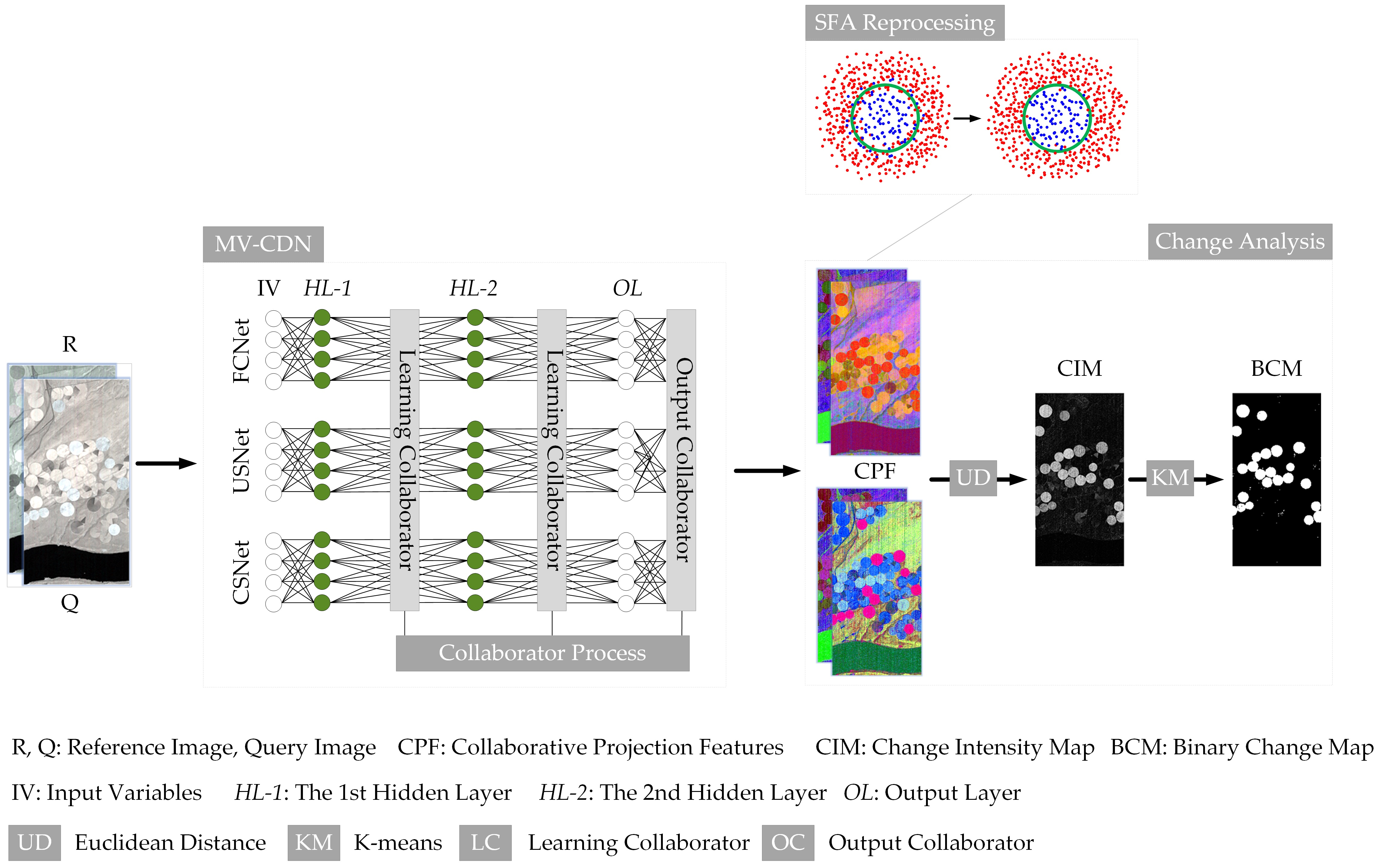
• This section describes the procedure of the proposed schema, which is composed of four modules: the MV-CDN module, the collaborator module, the SFA reprocessing module, and the change analysis model.
• The MV-CDN consists of three subdivision approaches: CDN-C, CDN-2C, and CDN-3C, with CDN-C denoting the CDN with one collaborator on the OL, CDN-2C denoting the CDN with two collaborators on the OL and HL-2, and CDN-3C denoting the CDN with three collaborators on the OL, HL-2, and HL-1.
• We first feed the double-channel MV-CDN with symmetric training pixels X and Y, which are selected from specific areas of the pre-detected binary change map (BCM) obtained from DSFA [25] with SFA reprocessing omitted, and the specific areas are detailed in the experiment section. The MV-CDN model could be well-trained following Section 3.1 and Section 3.2 under the hyperparameter settings in the experimental section. In the deep learning process, three light-weight collaborative network members, FCNet [25], USNet [26], and CSNet [26], are employed to serve the MV-CDN; the SFA algorithm is applied to construct the loss function for extracting invariance features. As the central idea of this paper, collaborators are utilized to translate the group-thinking of the collaborative network members into a more robust field of vision.
• The collaborators carried by different network layers of the three subdivision approaches are shown in Table 1, where OC denotes the output collaborator and LC denotes the learning collaborator.
• Figure 1 shows the procedure of the proposed schema for detecting the changes of double-temporal hyperspectral images. Given the reference image denoted by R and query image denoted by Q, we reshape both into N × 1 × B-dimensional data, with N and B respectively denoting the number of pixels and the band number of an image. Note that N is equivalent to H × W, with H and W respectively representing the height and width of the image. All paired pixels will pass the well-trained model to obtain the CPF with a spatial dimension of H × W × b, with b denoting the number of feature bands. Next, the SFA reprocessing module is employed to further inhibit the unchanged features and enhance the changed features of the spatial data model of N × 1 × b. Finally, in the change-analysis module, the Euclidean distance [34] and K-means [28] algorithms are successively applied to compute the change-intensity map and the final binary change map.

Figure 1. Flowchart of proposed schema based on multi-visual collaborative deep network (MV-CDN), which consist of three collaborative network members: fully connected network (FCNet), unchanged sensitivity network (USNet), and changed sensitivity network (CSNet).

Figure 1. Flowchart of proposed schema based on multi-visual collaborative deep network (MV-CDN), which consist of three collaborative network members: fully connected network (FCNet), unchanged sensitivity network (USNet), and changed sensitivity network (CSNet).

3.1. Architecture and Training Process of Proposed MV-CDN

In this section we describe the architecture of the MV-CDN and explain it mathematically in detail. The MV-CDN consists of three light-weight collaborative network members with similar structures and sensitivity disparity. In this work, the FCNet [25] is regarded as the prototype of the particular collaborative network members. Extensive experiments have confirmed that the double-cycle of internal parameters W and b in the HL-1/HL-2 is more conducive to detecting changed pixels/unchanged pixels. Thus far, the construction of the USNet and CSNet, which we have proposed in our previous work [26], is designed and implemented. Supposing there is no collaborator, each collaborative network member can independently generate the projection features for the change-detection analysis; with the MV-CDN mechanism, the collaborators are selectively applied to translate the group-thinking of the collaborative network members into a more robust field of vision.

We illustrate the architecture of the collaborative network members, FCNet, USNet, and CSNet, in Figure 2 and demonstrate their corresponding parameter settings in

Table 2. Cycle layers of internal parameters and structural configuration of some hyperparameters for collaborative network members: FCNet, USNet, and CSNet.

Settings		Activation Function	Nodes	Double-Cycle	Dropout
FCNet	IV	N/A	B	N/A	N/A
	HL-1	$\mathrm{Softsign}$	128	×	0
	HL-2	$\mathrm{Softsign}$	128	×
	OL	$\mathrm{Softsign}$	6	×
USNet	IV	N/A	B	N/A	N/A
	HL-1	$\mathrm{Leaky}\_\mathrm{relu}$	128	×	0.2
	HL-2	$\mathrm{Softsign}$	128	√
	OL	$\mathrm{Tan}\mathrm{h}$	10	×
CSNet	IV	N/A	B	N/A	N/A
	HL-1	$\mathrm{Leaky}\_\mathrm{relu}$	128	√	0.2
	HL-2	$\mathrm{Softsign}$	128	×
	OL	$\mathrm{Tan}\mathrm{h}$	10	×

. In Figure 2, the white nodes on the far left, denoted by X and Y, indicate the input variables (IV) of the double-temporal samples; the rightmost white nodes denoted by ${\mathrm{X}}^f$/${\mathrm{X}}^u$/${\mathrm{X}}^c$ and ${\mathrm{Y}}^f$/${\mathrm{Y}}^u$/${\mathrm{Y}}^c$ indicate the symmetric projection features of the collaborative network members: FCNet denoted as f, USNet denoted as u, and CSNet denoted as c; the green nodes on the rightmost stand for the output layer; consequently, the remaining two groups of green nodes represent the two hidden layers. In Table 2, the 128, 6, and 10 indicate the numbers of nodes; B and b indicate the number of bands of each detected image and the number of bands of the corresponding mapped features, respectively. Table 2 also lists the cycle layers, the activation function of each layer, and the dropout rate. Additionally, the learning rate, epoch, sampling range, and sample size, etc., are detailed in the experimental section.

We feed the symmetric samples X and Y to train the MV-CDN. The well-designed process of HL-1 is formulated in proper order as (1)–(3).

$$\begin{array}{c}{\mathrm{X}}_{HL-1}^f=a_{HL-1}^f\left({\mathrm{W}}_{HL-1}^f\mathrm{X}+b_{HL-1}^f\right)\\ {\mathrm{Y}}_{HL-1}^f=a_{HL-1}^f\left({\mathrm{W}}_{HL-1}^f\mathrm{Y}+b_{HL-1}^f\right)\end{array}$$

(1)

$$\begin{array}{c}{\mathrm{X}}_{HL-1}^u=a_{HL-1}^u\left({\mathrm{W}}_{HL-1}^u\mathrm{X}+b_{HL-1}^u\right)\\ {\mathrm{Y}}_{HL-1}^u=a_{HL-1}^u\left({\mathrm{W}}_{HL-1}^u\mathrm{Y}+b_{HL-1}^u\right)\end{array}$$

(2)

$$\begin{array}{c}{\mathrm{X}}_{HL-1}^c=a_{HL-1}^c\left({\mathrm{W}}_{HL-1}^c\left(a_{HL-1}^c\left({\mathrm{W}}_{HL-1}^c\mathrm{X}+b_{HL-1}^c\right)\right)+b_{HL-1}^c\right)\\ {\mathrm{Y}}_{HL-1}^c=a_{HL-1}^c\left({\mathrm{W}}_{HL-1}^c\left(a_{HL-1}^c\left({\mathrm{W}}_{HL-1}^c\mathrm{Y}+b_{HL-1}^c\right)\right)+b_{HL-1}^c\right)\end{array}$$

(3)

where f, u, and c respectively indicate the three collaborative network members: FCNet, USNet, and CSNet; $a_{HL-1}^f$, $a_{HL-1}^u$, and $a_{HL-1}^c$ are the corresponding activation functions, $a_{HL-1}^f=\mathrm{Softsign}$, $a_{HL-1}^c,a_{HL-1}^u=\mathrm{Leaky}\_\mathrm{Relu}$; the superscript and subscript of internal parameters W and b indicate the collaborative network members and the current layer, respectively; and the paired results $\left({\mathrm{X}}_{HL-1}^f,{\mathrm{Y}}_{HL-1}^f\right)$, $\left({\mathrm{X}}_{HL-1}^u,{\mathrm{Y}}_{HL-1}^u\right)$, and $\left({\mathrm{X}}_{HL-1}^c,{\mathrm{Y}}_{HL-1}^c\right)$ are three outputs of the corresponding layer of the collaborative network members.

In the CDN-3C approach, the outputs of HL-1 will then go through the LC of the collaborator process module to obtain the pair-wise data $\left({\mathrm{X}}_{HL-1}^{upd},{\mathrm{Y}}_{HL-1}^{upd}\right)$, which are taken as the input of HL-2, where ‘upd’ means ‘updated’. However, in the case of the other two subdivision approaches, the output of HL-1 is regarded as the input of HL-2. With LC, the HL-2 process can be represented as (4)–(6).

$$\begin{array}{c}{\mathrm{X}}_{HL-2}^f=a_{HL-2}^f\left({\mathrm{W}}_{HL-2}^f{\mathrm{X}}_{HL-1}^{upd}+b_{HL-2}^f\right)\\ {\mathrm{Y}}_{HL-2}^f=a_{HL-2}^f\left({\mathrm{W}}_{HL-2}^f{\mathrm{Y}}_{HL-1}^{upd}+b_{HL-2}^f\right)\end{array}$$

(4)

$$\begin{array}{c}{\mathrm{X}}_{HL-2}^u=a_{HL-2}^u\left({\mathrm{W}}_{HL-2}^u\left(a_{HL-2}^u\left({\mathrm{W}}_{HL-2}^u{\mathrm{X}}_{HL-1}^{upd}+b_{HL-2}^u\right)\right)+b_{HL-2}^u\right)\\ {\mathrm{Y}}_{HL-2}^u=a_{HL-2}^u\left({\mathrm{W}}_{HL-2}^u\left(a_{HL-2}^u\left({\mathrm{W}}_{HL-2}^u{\mathrm{Y}}_{HL-1}^{upd}+b_{HL-2}^u\right)\right)+b_{HL-2}^u\right)\end{array}$$

(5)

$$\begin{array}{c}{\mathrm{X}}_{HL-2}^c=a_{HL-2}^c\left({\mathrm{W}}_{HL-2}^c{\mathrm{X}}_{HL-1}^{upd}+b_{HL-2}^c\right)\\ {\mathrm{Y}}_{HL-2}^c=a_{HL-2}^c\left({\mathrm{W}}_{HL-2}^c{\mathrm{Y}}_{HL-1}^{upd}+b_{HL-2}^c\right)\end{array}$$

(6)

where $a_{HL-2}^f$, $a_{HL-2}^u$, and $a_{HL-2}^c$ are the corresponding activation functions, $a_{HL-2}^f,a_{HL-2}^c,a_{HL-2}^u=\mathrm{Softsign}$. Likewise, in the CDN-3C and CDN-2C approaches, the LC of the collaborator process module is used to obtain the updated paired data $\left({\mathrm{X}}_{HL-2}^{upd},{\mathrm{Y}}_{HL-2}^{upd}\right)$, which will then go through the output layer to obtain the projection features. In the case of CDN-C approach, the output of HL-2 is regarded as the input of the output layer. With LC, the process of the output layer can be expressed with (7)–(9).

$$\begin{array}{c}{\mathrm{X}}_{OL}^f=a_{OL}^f\left({\mathrm{W}}_{OL}^f{\mathrm{X}}_{HL-2}^{upd}+b_{OL}^f\right)\\ {\mathrm{Y}}_{OL}^f=a_{OL}^f\left({\mathrm{W}}_{OL}^f{\mathrm{Y}}_{HL-2}^{upd}+b_{OL}^f\right)\end{array}$$

(7)

$$\begin{array}{c}{\mathrm{X}}_{OL}^u=a_{OL}^u\left({\mathrm{W}}_{OL}^u{\mathrm{X}}_{HL-2}^{upd}+b_{OL}^u\right)\\ {\mathrm{Y}}_{OL}^u=a_{OL}^u\left({\mathrm{W}}_{OL}^u{\mathrm{Y}}_{HL-2}^{upd}+b_{OL}^u\right)\end{array}$$

(8)

$$\begin{array}{c}{\mathrm{X}}_{OL}^c=a_{OL}^c\left({\mathrm{W}}_{OL}^c{\mathrm{X}}_{HL-2}^{upd}+b_{OL}^c\right)\\ {\mathrm{Y}}_{OL}^c=a_{OL}^c\left({\mathrm{W}}_{OL}^c{\mathrm{Y}}_{HL-2}^{upd}+b_{OL}^c\right)\end{array}$$

(9)

where $a_{OL}^f$, $a_{OL}^u$, and $a_{OL}^c$ are the corresponding activation functions, $a_{OL}^f=\mathrm{Softsign}$, $a_{OL}^c,a_{OL}^u=\mathrm{Tanh}$. Afterwards, OC is applied on the output layer to calculate the pair-wise CPF $\left({\mathrm{X}}_{OL}^{new},{\mathrm{Y}}_{OL}^{new}\right)$, which are then used for further change analysis, where ‘new’ means the new matrix updated from the projection features of the collaborative network members.

To train the MV-CDN model, we follow the loss function of DSFA [25], which is derived from the feature invariance extraction known as SFA theory on double-temporal images. The SFA theory is summarized into an objective function and three restrictions [25], which could be reconstructed into a generalized eigenproblem as (10).

$$\mathrm{AW}=\mathrm{BWL}$$

(10)

where W and L stand for the generalized eigenvector matrix and diagonal matrix of eigenvalues, respectively; A and B denote the expectation of the covariance matrix for the first-order derivative of double-temporal features and the expectation of the covariance matrix for double-temporal features as (11) and (12), respectively.

$$\begin{array}{cc}\mathrm{A}\hfill & =\frac{1}{n}{\displaystyle \sum _{i=1}^n\left(x_i-y_i\right){\left(x_i-y_i\right)}^{\mathrm{T}}}\hfill \\ & =\sum \mathrm{XY}\hfill \end{array}$$

(11)

$$\begin{array}{cc}\mathrm{B}& =\frac{1}{2n}\left({\displaystyle \sum _{i=1}^n{x}_i}{x}_i^{\mathrm{T}}+{\displaystyle \sum _{i=1}^n{y}_i}{y}_i^{\mathrm{T}}\right)\hfill \\ & =\frac{1}{2}\left(\sum \mathrm{XX}+\sum \mathrm{YY}\right)\hfill \end{array}$$

(12)

where $x_i$ and $y_i$ are regarded as the ith pair-wise pixels; T and n indicate the transpose operation and the number of pixels of a whole image. In conditions where both $\sum \mathrm{XX}$ and $\sum \mathrm{YY}$ are non-negative and invertible, the generalized eigenproblem can be reformulated as (13).

$${\mathrm{B}}^{-1}\mathrm{AW}=\mathrm{WL}$$

(13)

where the square of ${\mathrm{B}}^{-1}\mathrm{A}$ should be minimized to meet the feature invariance of SFA theory; thus, the loss function could be designed as (14).

$$Loss\left[\left({\mathrm{W}}_{\mathrm{X}},b_{\mathrm{X}}\right),\left({\mathrm{W}}_{\mathrm{Y}},b_{\mathrm{Y}}\right)\right]=tr\left[{\left({\mathrm{B}}^{-1}\mathrm{A}\right)}^2\right]$$

(14)

where tr denotes the trace of the matrix. Through the gradient descent algorithm detailed in part B of the methodology section of reference [25], both pair-wise internal parameters $\left({\mathrm{W}}_{\mathrm{X}},b_{\mathrm{X}}\right)$ and $\left({\mathrm{W}}_{\mathrm{Y}},b_{\mathrm{Y}}\right)$, which result from the learning of X and Y, are obtained.

3.2. Collaborator Process

In this section, Figure 3 shows the collaborator process of subdivision approaches. In HL-1 and HL-2, LC is applied for the collaborative task, which is formulated as (15)–(17), and before that the data of tensor type to be processed should be converted to array type.

$$\left.\begin{array}{l}Min\left(d\left({\mathrm{x}}_i^f{,\mathrm{x}}_i^u\right),d\left({\mathrm{x}}_i^f{,\mathrm{x}}_i^c\right),d\left({\mathrm{x}}_i^u{,\mathrm{x}}_i^c\right)\right)\\ Min\left(d\left({\mathrm{y}}_i^f{,\mathrm{y}}_i^u\right),d\left({\mathrm{y}}_i^f{,\mathrm{x}}_i^c\right),d\left({\mathrm{y}}_i^u{,\mathrm{y}}_i^c\right)\right)\end{array}\right\}\Rightarrow \left\{\begin{array}{l}(x_i^a,x_i^b)\\ (y_i^a,y_i^b)\end{array}\right.$$

(15)

where i and d denote the pixel index and the absolute value of the difference between two values, respectively; Min is an operator to take the minimum of three values; in the obtained $(x_i^a,x_i^b)$ and $(y_i^a,y_i^b)$, the pair (a, b) is regarded as one of three pairs: (f, u), (f, c), and (u, c). Then, (16) is used for the revaluation of $(x_i^a,x_i^b)$ and $(y_i^a,y_i^b)$.

$$\left.\begin{array}{l}Mean(x_i^a,x_i^b)\\ Mean(y_i^a,y_i^b)\end{array}\right\}\Rightarrow \left\{\begin{array}{l}{\mathrm{X}}_{HL-j}^{new}\\ {\mathrm{Y}}_{HL-j}^{new}\end{array}\right.$$

(16)

where Mean represents the arithmetic average operator, HL-j signifies the jth hidden layer, and naturally, the paired data $\left({\mathrm{X}}_{HL-j}^{new},{\mathrm{Y}}_{HL-j}^{new}\right)$ denote the re-evaluation results of the full image in HL-j. To realize the network transmission, (17) is utilized to convert the new results to tensor type without destroying the calculation graph.

$$\begin{array}{c}{\mathrm{X}}_{HL-j}^{upd}{=\mathrm{X}}_{HL-j}^u{ \ast \mathrm{mask}+\mathrm{X}}_{HL-j}^{new\_tnr} \ast (1-\mathrm{mask})\\ {\mathrm{Y}}_{HL-j}^{upd}{=\mathrm{Y}}_{HL-j}^u{ \ast \mathrm{mask}+\mathrm{Y}}_{HL-j}^{new\_tnr} \ast (1-\mathrm{mask})\end{array}$$

(17)

where the pair-wise data $\left({\mathrm{X}}_{HL-j}^u,{\mathrm{Y}}_{HL-j}^u\right)$ act as two motherboard tensors; $\left({\mathrm{X}}_{HL-j}^{new\_tnr}{, \mathrm{Y}}_{HL-j}^{new\_tnr} \right)$ stands for the tensor type of $\left({\mathrm{X}}_{HL-j}^{new},{\mathrm{Y}}_{HL-j}^{new}\right)$, which has been obtained with (16); the mask is a binary matrix whose dimension is consistent with each tensor of paired data $\left({\mathrm{X}}_{HL-j}^u,{\mathrm{Y}}_{HL-j}^u\right)$. Moreover, in practice, all feature elements are regarded as updated; thus, the mask ought to be filled with 0. We calculate the Hadamard product on the pair-wise data $\left({\mathrm{X}}_{HL-j}^u,{\mathrm{Y}}_{HL-j}^u\right)$ and mask, then add the tensor type of the paired data $\left({\mathrm{X}}_{HL-j}^{new},{\mathrm{Y}}_{HL-j}^{new}\right)$ marked with $\left({\mathrm{X}}_{HL-j}^{new\_tnr}{, \mathrm{Y}}_{HL-j}^{new\_tnr}\right)$ to obtain the needed results ${\mathrm{X}}_{HL-j}^{upd}$ and ${\mathrm{Y}}_{HL-j}^{upd}$, which are regarded as the input of the next layer. In (17), the ‘upd’ and ‘new_tnr’ mean ‘updated’ and ‘new_tensor’, respectively. We especially note that the other two pairs of data $\left({\mathrm{X}}_{HL-j}^f,{\mathrm{Y}}_{HL-j}^f\right)$ and $\left({\mathrm{X}}_{HL-j}^c,{\mathrm{Y}}_{HL-j}^c\right)$ could also be taken as motherboard tensors and are involved with computing; in particular, we test with the pair-wise data $\left({\mathrm{X}}_{HL-j}^u,{\mathrm{Y}}_{HL-j}^u\right)$ in the collaborator process.

Regarding the output layer, since the projection features no longer transmit in the network, (15) and (16) are utilized with (17) omitted to calculate the pair-wise data $\left({\mathrm{X}}_{OL}^{new},{\mathrm{Y}}_{OL}^{new}\right)$.

3.3. SFA Reprocessing

In the tests we feed the well-trained model with a reference image R and query image Q to obtain the double-temporal CPF $\left({\mathrm{R}}_1{,\mathrm{Q}}_1\right)$. To take the SFA efficiency one step further, the weight vector matrix W resulting from USNet is required because the USNet is more sensitive to unchanged pixels to match the SFA objectives. The SFA reprocessing can further inhibit the unchanged features to highlight the changed features as conducive to the segmentation of thresholding.

As shown in Figure 4a, before SFA reprocessing with the effective network, the red dots and blue dots of reverse scattering would undoubtedly lead to false segmentation. To execute the SFA reprocessing, we multiply the transpose of W with $\left({\mathrm{R}}_1{,\mathrm{Q}}_1\right)$ as in (18) to produce the feature sets $\left({\mathrm{R}}_2{,\mathrm{Q}}_2\right)$. The result is indicated as Figure 4b. It is noteworthy that the effectiveness of SFA reprocessing depends on the expressiveness of the network used in the previous step; thus, the deep features of low quality would reinforce the error description, as described in Figure 4c,d.

$${\mathrm{R}}_2{=\mathrm{W}}^{\mathrm{T}}{\mathrm{R}}_1{, \mathrm{Q}}_2{=\mathrm{W}}^{\mathrm{T}}{\mathrm{Q}}_1$$

(18)

3.4. Change Analysis

In effect, it is impossible to artificially recognize the change areas from the double-temporal features $\left({\mathrm{R}}_2{,\mathrm{Q}}_2\right)$. Therefore, the Chi-square distance [35], Euclidean distance [34] and improved Mahalanobis distance [36], etc., could be selectively applied to the calculation of the change-intensity map (CIM). In the tests, the Euclidean distance is employed to serve the computing of CIM using (19) and (20).

$$\mathrm{CIM}=\sqrt{{\mathrm{Diff}}^{\mathrm{T}}\mathrm{Diff}}$$

(19)

$$\mathrm{Diff}={\displaystyle \sum _{j=1}^b{\displaystyle \sum _{i=1}^n\left(r_{(i,j)}-q_{(i,j)}\right)}}$$

(20)

where $i$, $j$, $n$, and $b$ stand for the pixel index, the band index, the number of pixels, and the number of bands, respectively. The $r_{(i,j)}$ and $q_{(i,j)}$ indicate the feature elements acquired from the pair-wise data ${\mathrm{R}}_2$ and ${\mathrm{Q}}_2$, respectively.

The computed result of Euclidean distance is regarded as the CIM, which could be applied for the initial detection of changes. Then the K-means clustering method is employed as automatic thresholding for image segmentation, and finally the binary change map is generated, in which the white and black marks uniquely identify the changed and unchanged areas, respectively. The pseudocode of the proposed schema is summarized and presented in Algorithm 1.

Algorithm 1 Pseudocode of proposed schema for change detection of double-temporal hyperspectral images

Input: Double-temporal scene images R and Q;

Output: Detected binary change map (BCM);

1:  Select training samples X and Y based on BCM of pre-detection;

2:  Initialize parameters of MV-CDN as ${\mathrm{P}}_{\mathrm{X}},$ ${\mathrm{P}}_{\mathrm{Y}}$;

3:  Configuration of epoch number, learning rate, sample size, etc.;

4:  Case CDN-C:

5:    Apply OC on OL;

6:    Go to line 13;

7:  Case CDN-2C:

8:    Apply OC on OL, and LC on HL-2;

9:    Go to line 13;

10: Case CDN-3C:

11:    Apply OC on OL, and LC on HL-2& HL-1;

12:    Go to line 13;

13: while i < epochs do

14:    Compute the double-temporal projection features of pair-wise samples X and Y: $\hat{\mathrm{X}}$ = f (X, ${\mathrm{P}}_{\mathrm{X}}$) and $\hat{\mathrm{Y}}$ = f (Y, ${\mathrm{P}}_{\mathrm{Y}}$);

15:    Compute the gradient of loss function $L$(${\mathrm{P}}_{\mathrm{X}},$ ${\mathrm{P}}_{\mathrm{Y}}$) = $\mathrm{tr}[{\left({\left(\hat{\mathrm{B}}\right)}^{-1}\hat{\mathrm{A}}\right)}^2]$ with $\partial$L$({\mathrm{P}}_{\mathrm{X}},$ ${\mathrm{P}}_{\mathrm{Y}}$)/$\partial {\mathrm{P}}_{\mathrm{X}}$ and $\partial$L (${\mathrm{P}}_{\mathrm{X}},$ ${\mathrm{P}}_{\mathrm{Y}}$)/$\partial {\mathrm{P}}_{\mathrm{Y}}$;

16:    Update parameters;

17:    i++;

18: end

19: Generate the double-temporal projection features ${\mathrm{R}}_1$ and ${\mathrm{Q}}_1$ of images R and Q;

20: SFA reprocessing is applied to the CPF to generate the pair-wise data $\left({\mathrm{R}}_2{,\mathrm{Q}}_2\right)$ with: ${\mathrm{R}}_2{=\mathrm{W}}^{\mathrm{T}}{\mathrm{R}}_1$, ${\mathrm{Q}}_2{=\mathrm{W}}^{\mathrm{T}}{\mathrm{Q}}_1$;

21: Euclidean distance is used for the calculation of CIM;

22: K-means is applied to obtain the BCM;

23: return BCM;

In the tests, we found that other distance methods have little influence on the detection results in comparison to the using of Euclidean distance; in addition, the K-means clustering algorithm could be replaced by other threshold algorithms such as Otsu [37]. In particular, the designed example uniformly adopts the Euclidean distance and K-means threshold algorithm.

4. Results

To test the performance of comparison methods, three hyperspectral image datasets acquired from web address [38] are employed. We detail the tested datasets as follows. As shown in Figure 5, all three datasets are double-temporal data models. Among them, the scene images of “Hermiston” were taken in 2004 and 2007. It covers Hermiston City, Oregon, with a 30 m ground resolution using the HYPERION sensor and a size of 390 × 200 pixels. There are 242 spectral bands selected for change-detection tasks. The full image of Hermiston is labelled with 78,000 pixels, including 9986 positive pixels and 68,014 negative pixels. The two hyperspectral images of the dataset “Santa Barbara” were obtained from the AVIRIS sensor in 2013 and 2014 over Santa Barbara, California, USA, with a 20 m ground resolution and having a spatial dimension of 984 × 740 × 224 to indicate the height and width of pixels and the number of bands, respectively. The “Bay Area” scenes were acquired using the AVIRIS sensor in 2013 and 2015 over Patterson City, California, USA, with a 20 m ground resolution and dimensional size of 600 × 500 × 224. It is estimated that the full image of the Santa Barbara dataset has 728,160 pixels, including 52,134 positive pixels, 80,418 negative pixels, and 595,608 unlabeled pixels; while in the ‘Bay Area dataset, there are 300,000 pixels in each image, including 39,270 positive pixels, 34,211 negative pixels, and 226,519 unlabeled pixels.

4.1. Measurement Coefficients

Figure 5(C3) demonstrates the ground-truth maps of the tested datasets. Among them, the white marks and black marks of (R2, C3) indicate the positives and negatives, respectively, while in (R1, C3) and (R3, C3), the silver marks and white marks represent the labelled areas, with silver marks denoting the negatives and white marks representing the positives. Based on the ground-truth maps with confidence of absoluteness, five metric coefficients, OA_CHG, OA_UN, OA [39], Kappa and F1 [40], as defined in (21)–(26), are employed to quantify the comparison among methods of change detection.

$$\mathrm{OA}\_\mathrm{CHG}=\frac{\mathrm{TP}}{\mathrm{LP}}$$

(21)

$$\mathrm{OA}\_\mathrm{UN}=\frac{\mathrm{TN}}{\mathrm{LN}}$$

(22)

$$\mathrm{OA}=\frac{\mathrm{TP}+\mathrm{TN}}{\mathrm{ALL}}$$

(23)

$$\mathrm{Kappa}=\frac{\mathrm{OA}-\mathrm{Pe}}{1-\mathrm{Pe}}$$

(24)

$$\mathrm{Pe}=\frac{(\mathrm{TP}+\mathrm{FP})\times \mathrm{LP}+(\mathrm{TN}+\mathrm{FN})\times \mathrm{LN}}{{\mathrm{ALL}}^2}$$

(25)

$$\mathrm{F}1=\frac{2\mathrm{TP}}{2\mathrm{TP}+\mathrm{FP}+\mathrm{FN}}$$

(26)

where OA_CHG and OA_UN are two metric coefficients on positive pixels and negative pixels, respectively, while OA, Kappa, and F1 are three comprehensive coefficients of different measurement modes. In the equations, ALL stands for the total number of labelled pixels; TP and FN indicate the number of true positives and false negatives, respectively, and the sum of them is equivalent to LP, which means the number of labelled positives; TN and FP represent the number of true negatives and false positives, respectively, and their sum is equivalent to LN, which signifies the number of labelled negatives.

With respect to the hyperparameters, the number of nodes of each hidden layer denoted by NoH, the number of nodes of the output layer represented by NoO, and the learning rate (LR) are, respectively, $5\times {10}^{-5}$, 128, and 10. In clinical practice, the pair-wise pixels matched to the specific areas are regarded as training samples. Hence, in the tests, the pre-detected binary change map (PD-BCM) resulting from the change-detection model using the fully connected network (CD-FCNet) [25] and with SFA reprocessing cancelled is applied as the sampling reference object. Furthermore, because of the synchronous collaboration, all collaborative network members train with 2000 epochs. The dataset Santa Barbara requires 3000 paired pixels selected from the changed areas of PD-BCM, while 3000 paired pixels of unchanged areas are selected for the other two datasets, Hermiston and Bay Area. We especially note that the visualization and quantization results of a particular dataset are generated from the same sampling strategy; therefore, the comparison is fair.

When the training of the MV-CDN is completed, two detected images are fed to the well-trained model to generate three couples of CPF for three subdivision approaches, CDN-C, CDN-2C, and CDN-3C. Since an RGB image has three bands, we endow the fourth, third, and second bands to synthesize the feature map of pseudo-color from CPF. By performing the comparison methods on three tested datasets, we demonstrate the double-temporal feature maps of CPF in Figure 6, where the left column, right column, top row, and bottom row are assigned to the feature maps resulting from the reference image and query image with and without SFA reprocessing, respectively. (C1)–(C6) correspond respectively to the comparison methods: DSFA [25], the change-detection model using the unchanged sensitivity network (CD-USNet) [26], the change-detection model using the changed sensitivity network (CD-CSNet) [26], and the proposed CDN-C, CDN-2C, and CDN-3C.

In Figure 7, Figure 8 and Figure 9, (R1) demonstrates the divergence maps; (R2) shows the change-intensity maps (CIM), with very bright marks indicating a change of high probability and very dark marks denoting a small change or no change. In the grayscale CIM, it is difficult to determine the pixel-wise change states. Therefore, the K-means clustering algorithm is then applied to generate the BCM as shown in (R3), where the white marks and black marks represent the detected changed areas and unchanged areas, respectively. To identify the detected states of TP, FN, TN, and FP, as well as the unlabeled domain, we recolor the BCM with white, red, green, yellow, and black, respectively, to generate the hitting state map (HSM), as shown in (R4). Since the dataset Hermiston does not contain an unlabeled domain, there exist no black marks in the corresponding HSM.

4.2. Comparison with State-of-the-Art Work

This part analyzes and compares the proposed scheme and the state-of-the-art work: DSFA [25], CD-USNet [26], and CD-CSNet [26] in the perspectives of visualization and quantitation. Figure 7, Figure 8 and Figure 9 shows the visualization results on the three datasets Hermiston, Santa Barbara, and Bay Area, respectively.

In Figure 7, (R4, C4), (R5, C4), and (R6, C4), and in Figure 8 and Figure 9, (R4, C4), (R4, C5), and (R4, C6) are the three images with the smallest area of red marks and largest area of white marks, representing the minimum FN values and maximum TP values, respectively. This also indicates that the proposed scheme is a method to obtain a high hit-rate of changed pixels in comparison to the benchmarks. Moreover, a closer examination reveals that, even if the proposed schema does not always have the superiority in detecting unchanged pixels, due to its distinct advantage on changed pixels, it always outperforms the benchmarks in overall performance.

The five well-formulated coefficients OA_CHG, OA_UN, OA, Kappa, and F1 given in (21)–(26) were calculated to show the performance of the change-detection methods. Reliable and high-quality data are provided for analysis in

Table 3. Comparison of quantization results on dataset Hermiston.

	Results	TP	TN	FP	FN	OA_CHG	OA_UN	OA	Kappa	F1
	DSFA [25]	9299	67,467	547	687	0.9312	0.9920	0.9842	0.9287	0.9378
	CD-USNet [26]	9206	67,650	364	780	0.9219	0.9946	0.9853	0.9331	0.9415
	CD-CSNet [26]	9314	67,535	479	672	0.9327	0.9930	0.9852	0.9334	0.9418
CD-SDN	CD-SDN-AM [26]	9195	67,674	340	791	0.9208	0.9950	0.9855	0.9338	0.9421
	CD-SDN-AL [26]	9346	67,632	382	640	0.9359	0.9944	0.9869	0.9407	0.9482
MV-CDN	CDN-C (Proposed)	9420	67,578	436	566	0.9433	0.9936	0.9872	0.9421	0.9495
	CDN-2C (Proposed)	9414	67,597	417	572	0.9427	0.9939	0.9873	0.9428	0.9501
	CDN-3C (Proposed)	9456	67,543	471	530	0.9469	0.9931	0.9872	0.9424	0.9497

,

Table 4. Comparison of quantization results on dataset Santa Barbara.

	Results	TP	TN	FP	FN	OA_CHG	OA_UN	OA	Kappa	F1
	DSFA [25]	43,426	79,333	1085	8708	0.8330	0.9865	0.9261	0.8411	0.8987
	CD-USNet [26]	43,442	79,580	838	8692	0.8333	0.9896	0.9281	0.8452	0.9012
	CD-CSNet [26]	45,497	77,087	3331	6637	0.8727	0.9586	0.9248	0.8406	0.9013
CD-SDN	CD-SDN-AM [26]	46,532	76,838	3580	5602	0.8925	0.9555	0.9307	0.8539	0.9102
	CD-SDN-AL [26]	45,481	78,892	1526	6653	0.8724	0.9810	0.9383	0.8684	0.9175
MV-CDN	CDN-C (Proposed)	45,547	78,855	1563	6587	0.8737	0.9806	0.9385	0.8689	0.9179
	CDN-2C (Proposed)	45,537	78,912	1506	6597	0.8735	0.9813	0.9389	0.8697	0.9183
	CDN-3C (Proposed)	45,593	78,781	1637	6541	0.8745	0.9796	0.9383	0.8685	0.9177

and

Table 5. Comparison of quantization results on dataset Bay Area.

	Results	TP	TN	FP	FN	OA_CHG	OA_UN	OA	Kappa	F1
	DSFA [25]	32,972	32,961	1250	6298	0.8396	0.9635	0.8973	0.7955	0.8973
	CD-USNet [26]	32,959	33,042	1169	6311	0.8393	0.9658	0.8982	0.7974	0.8981
	CD-CSNet [26]	33,738	32,603	1608	5532	0.8591	0.9530	0.9028	0.8062	0.9043
CD-SDN	CD-SDN-AM [26]	35,717	31,815	2396	3553	0.9095	0.9300	0.9190	0.8377	0.9231
	CD-SDN-AL [26]	35,632	32,422	1789	3638	0.9074	0.9477	0.9261	0.8521	0.9292
MV-CDN	CDN-C (Proposed)	35,654	32,618	1593	3616	0.9079	0.9534	0.9291	0.8581	0.9319
	CDN-2C (Proposed)	35,645	32,681	1530	3625	0.9077	0.9553	0.9298	0.8596	0.9326
	CDN-3C (Proposed)	35,590	32,675	1536	3680	0.9063	0.9551	0.9290	0.8579	0.9317

, where the more recent advanced algorithms, CD-SDN-AM and CD-SDN-AL [26], are compared, with the best result of each quantization coefficient marked in bold. We summarize the data analysis as follows. (1) Collaborative network members serving the MV-CDN are theoretically effective: based on the DSFA algorithm, the CD-CSNet model outperforms the DSFA in OA_CHG, while it underperforms in the OA_UN coefficient, and the CD-USNet model has been proved to be contrary. (2) Due to the characteristics of multi-vision, the MV-CDN model achieves a better balance in the detection performance of positive and negative pixels. (3) The proposed schema has intense, comparative, and slight superiority over the other comparison methods on the datasets Bay Area, Santa Barbara, and Hermiston, respectively. (4) Compared with CDN-2C, the CDN-3C with one more collaborator cannot further improve the detection performance. (5) Even though the proposed CDN-C and CDN-2C may not always be in the top two for the coefficients OA_CHG and OA_UN, their performance in the comprehensive coefficients OA, Kappa, and F1 is not inferior to any other method on any tested dataset.

On the platform of Tensorflow 2.0.0, Python 3.6.3, and with graphics hardware of NVIDIA GeForce RTX 3070 for each collaborative network member, the time costs of CDN-C, CDN-2C, and CDN-3C in the deep learning process were, respectively, 16 s, 21 s, and 28 s on dataset Hermiston; 25 s, 33 s, and 47s on dataset Santa Barbara; and 16 s, 22 s, and 29 s on dataset Bay Area, as demonstrated in Figure 10.

5. Discussion

The proposed MV-CDN is an effective deep model for change-detection tasks on double-temporal hyperspectral images. The subdivision approaches, CDN-2C and CDN-3C, are two collaborative deep models of compactness, because they restrict each other in the hidden layer(s). As we have shown, the CDN-3C, which takes the most time in the learning process with no improving performance, is an eliminated subdivision approach. The less time-consuming CDN-2C is not inferior to CDN-3C in terms of detection performance. Based on this, considering the performance and model compactness, CDN-2C is desirable. The CDN-C carries only one collaborator and takes the least time. In this case, the three collaborative network members have no mutual restriction before the output layer, and they do not even require a synchronized process or similar structure; thus, there is much variability in the collaborative network members when using CDN-C.

As we know, CDN-3C does not show performance superiority, whether in terms of detection accuracy or time consumption, compared to the other two approaches. The reasons can be explained as follows: (1) The mechanism of the proposed schema lies in the effective perspectives; however, in the HL-1, the transformation process of FCNet and USNet are the same, and this is reflected in Figure 2 and Table 2. In this case, the additional collaborator of the first hidden layer of CDN-3C may prevent the MV-CDN from generating better description features. (2) The sensitivity disparity between FCNet and USNet is formed until it reaches the HL-2, and therefore achieves a better multi-vision effect. (3) Within the effective range of perspectives (the second hidden layer and the output layer), CDN-2C outperforms the CDN-C because it has more collaborators.

6. Conclusions

In this paper, we propose a MV-CDN for double-temporal hyperspectral image change detection. In the proposed schema, three light-weight collaborative network members, the prototypical FCNet, USNet, and CSNet, are employed to serve three subdivision approaches: CDN-C, CDN-2C, and CDN-3C. In the CDN-C approach, an output collaborator is applied on the output layer; based on CDN-C, an additional learning collaborator is applied on the HL-2 for CDN-2C, while two additional learning collaborators are applied on HL-1 and HL-2 for CDN-3C. The collaborators integrate the multi-vision of three collaborative network members. When the collaborative projection features are acquired, the SFA reprocessing and Euclidean distance are successively applied to enlarge the difference between the changed pixels and unchanged pixels and then generate the change-intensity map. Finally, the K-means method is employed to split the change-intensity map into a binary change map, which can uniquely identify the detected changes. We implemented the proposed schema on three open double-temporal hyperspectral image datasets. The tested results show that our proposed scheme could outperform any change-detection model with a single collaborative network member and achieves a better balance in the detection performance of positive and negative pixels in comparison to the benchmarks.

References

1. Zheng, Z.; Wu, Z.; Chen, Y.; Yang, Z.; Marinello, F. Exploration of eco-environment and urbanization changes in coastal zones: A case study in China over the past 20 years. Ecol. Indic. 2020, 119, 106847. [Google Scholar] [CrossRef]
2. Yao, K.; Halike, A.; Chen, L.; Wei, Q. Spatiotemporal changes of eco-environmental quality based on remote sensing-based ecological index in the Hotan Oasis, Xinjiang. J. Arid. LandIssue 2022, 14, 262–283. [Google Scholar] [CrossRef]
3. Wang, L.; Li, R.; Zhang, C.; Fang, S.; Duan, C.; Meng, X.; Atkinson, P.M. UNetFormer: An UNet-like Transformer for Efficient Semantic Segmentation of Remote Sensing Urban Scene Imagery. SPRS J. Photogramm. Remote Sens. 2021, 190, 196–214. [Google Scholar] [CrossRef]
4. Rahman, A.; Aggarwal, S.P.; Netzband, M.; Fazal, S. Monitoring urban sprawl using remote sensing and GIS techniques of a fast growing urban centre, India. IEEE J. Sel. Top. Appl. Earth Obs. Remote Sens. 2010, 4, 56–64. [Google Scholar] [CrossRef]
5. Cao, C.; Dragićević, S.; Li, S. Land-use change detection with convolutional neural network methods. Environments 2019, 6, 25. [Google Scholar] [CrossRef]
6. Alhassan, V.; Henry, C.; Ramanna, S.; Storie, C. A deep learning framework for land-use/land-cover mapping and analysis using multispectral satellite imagery. Neural Comput. Appl. 2020, 32, 8529–8544. [Google Scholar] [CrossRef]
7. Wei, Z.; Gu, X.; Sun, Q.; Hu, X.; Gao, Y. Analysis of the Spatial and Temporal Pattern of Changes in Abandoned Farmland Based on Long Time Series of Remote Sensing Data. Remote Sens. 2021, 13, 2549. [Google Scholar] [CrossRef]
8. Sofia, G.; Bailly, J.-S.; Chehata, N.; Tarolli, P.; Levavasseur, F. Comparison of pleiades and LiDAR digital elevation models for terraces detection in farmlands. IEEE J. Sel. Top. Appl. Earth Obs. Remote Sens. 2016, 9, 1567–1576. [Google Scholar] [CrossRef]
9. Huang, Q.; Wang, C.; Meng, Y.; Chen, J.; Yue, A. Landslide Monitoring Using Change Detection in Multitemporal Optical Imagery. IEEE Geosci. Remote Sens. Lett. 2020, 17, 312–316. [Google Scholar] [CrossRef]
10. Lê, T.T.; Froger, J.-L.; Minh, D.H.T. Multiscale framework for rapid change analysis from SAR image time series: Case study of flood monitoring in the central coast regions of Vietnam. Remote Sens. Environ. 2022, 269, 112837. [Google Scholar] [CrossRef]
11. Liu, D.; Chen, W.; Menz, G.; Dubovyk, O. Development of integrated wetland change detection approach: In case of Erdos Larus Relictus National Nature Reserve, China. Sci. Total Environ. 2020, 731, 139166. [Google Scholar] [CrossRef]
12. Li, Y.; Dong, H.; Li, H.; Zhang, X.; Zhang, B. Multi-block SSD based on small object detection for UAV railway scene surveillance. Chin. J. Aeronaut. 2020, 33, 1747–1755. [Google Scholar] [CrossRef]
13. Zhu, Y.; Jia, Z.; Yang, J.; Kasabov, N.K. Change detection in multitemporal monitoring images under low illumination. IEEE Access 2020, 8, 126700–126712. [Google Scholar] [CrossRef]
14. Zhang, X.; Wu, H.; Wu, M.; Wu, C. Extended Motion Diffusion-Based Change Detection for Airport Ground Surveillance. IEEE Trans. Image Process. 2020, 29, 5677–5686. [Google Scholar] [CrossRef]
15. Zhao, Y.; Zhao, L.; Xiong, B.; Kuang, G. Attention receptive pyramid network for ship detection in SAR images. IEEE J. Sel. Top. Appl. Earth Obs. Remote Sens. 2020, 13, 2738–2756. [Google Scholar] [CrossRef]
16. Hou, Z.; Li, W.; Li, L.; Tao, R.; Du, Q. Hyperspectral Change Detection Based on Multiple Morphological Profiles. IEEE Trans. Geosci. Remote Sens. 2021, 60, 5507312. [Google Scholar] [CrossRef]
17. Wang, Y.; Hong, D.; Sha, J.; Gao, L.; Liu, L.; Zhang, Y.; Rong, X. Spectral–spatial–temporal transformers for hyperspectral image change detection. IEEE Trans. Geosci. Remote Sens. 2022, 60, 5536814. [Google Scholar] [CrossRef]
18. Afaq, Y.; Manocha, A. Analysis on change detection techniques for remote sensing applications: A review. Ecol. Inform. 2021, 63, 101310. [Google Scholar] [CrossRef]
19. Zhou, S.Q.; Schoellig, A.P. An Analysis of the Expressiveness of Deep Neural Network Architectures Based on Their Lipschitz Constants. arXiv 2019, arXiv:1912.11511. [Google Scholar]
20. Jeong, Y.S.; Byon, Y.J.; Castro-Neto, M.M.; Easa, S.M. Supervised Weighting-Online Learning Algorithm for Short-Term Traffic Flow Prediction. IEEE Trans. Intell. Transp. Syst. 2013, 14, 1700–1707. [Google Scholar] [CrossRef]
21. Blanchart, P.; Datcu, M. A Semi-Supervised Algorithm for Auto-Annotation and Unknown Structures Discovery in Satellite Image Databases. IEEE J. Sel. Top. Appl. Earth Obs. Remote Sens. 2010, 3, 698–717. [Google Scholar] [CrossRef]
22. Xu, J.; Zhao, R.; Yu, Y.; Zhang, Q.; Bian, X.; Wang, J.; Ge, Z.; Qian, D. Real-time automatic polyp detection in colonoscopy using feature enhancement module and spatiotemporal similarity correlation unit. Biomed. Signal Process. Control. 2022, 66, 102503. [Google Scholar] [CrossRef]
23. Zhang, P.; Xu, H.; Tian, T.; Gao, P.; Li, L.; Zhao, T.; Zhang, N.; Tian, J. SEFEPNet: Scale Expansion and Feature Enhancement Pyramid Network for SAR Aircraft Detection with Small Sample Dataset. IEEE J. Sel. Top. Appl. Earth Obs. Remote Sens. 2022, 15, 3365–3375. [Google Scholar] [CrossRef]
24. Qu, L.; Huang, S.; Jia, Y.; Li, X. Improved Loss Function-Based Prediction Method of Extreme Temperatures in Greenhouses. arXiv 2021, arXiv:2111.01366. [Google Scholar]
25. Du, B.; Ru, L.; Wu, C.; Zhang, L. Unsupervised deep slow feature analysis for change detection in multi-temporal remote sensing images. IEEE Trans. Geosci. Remote Sens. 2019, 57, 9976–9992. [Google Scholar] [CrossRef]
26. Li, J.; Yuan, X.; Li, J.; Huang, G.; Li, P.; Feng, L. CD-SDN: Unsupervised Sensitivity Disparity Networks for Hyper-Spectral Image Change Detection. Remote Sens. 2022, 14, 4806. [Google Scholar] [CrossRef]
27. Li, J.; Yuan, X.; Feng, L. Alteration Detection of Multispectral/Hyperspectral Images Using Dual-Path Partial Recurrent Networks. Remote Sens. 2021, 13, 4802. [Google Scholar] [CrossRef]
28. Kanungo, T.; Mount, D.M.; Netanyahu, N.S.; Piatko, C.D.; Silverman, R.; Wu, A.Y. An efficient k-means clustering algorithm: Analysis and implementation. IEEE Trans. Pattern Anal. Mach. Intell. 2002, 24, 881–892. [Google Scholar] [CrossRef]
29. Feng, S.; Fan, Y.; Tang, Y.; Cheng, H.; Zhao, C.; Zhu, Y.; Cheng, C. A Change Detection Method Based on Multi-Scale Adaptive Convolution Kernel Network and Multimodal Conditional Random Field for Multi-Temporal Multispectral Images. Remote Sens. 2022, 14, 5368. [Google Scholar] [CrossRef]
30. Yuan, Y.; Lv, H.; Lu, X. Semi-supervised change detection method for multi-temporal hyperspectral images. Neurocomputing 2015, 148, 363–375. [Google Scholar] [CrossRef]
31. Shi, Q.; Liu, M.; Li, S.; Liu, X.; Wang, F.; Zhang, L. A Deeply Supervised Attention Metric-Based Network and an Open Aerial Image Dataset for Remote Sensing Change Detection. IEEE Trans. Geosci. Remote Sens. 2022, 60, 5604816. [Google Scholar] [CrossRef]
32. Lei, J.; Li, M.; Xie, W.; Li, Y.; Jia, X. Spectral mapping with adversarial learning for unsupervised hyperspectral change detection. Neurocomputing 2021, 465, 71–83. [Google Scholar] [CrossRef]
33. Li, Q.; Gong, H.; Dai, H.; Li, C.; Mu, T. Unsupervised Hyperspectral Image Change Detection via Deep Learning Self-generated Credible Labels. IEEE J. Sel. Top. Appl. Earth Obs. Remote Sens. 2021, 14, 9012–9024. [Google Scholar] [CrossRef]
34. Danielsson, P.-E. Euclidean distance mapping. Comput. Graph. Image Process. 1980, 14, 227–248. [Google Scholar] [CrossRef]
35. Emran, S.M.; Ye, N. Robustness of Chi-square and Canberra distance metrics for computer intrusion detection. Qual. Reliab. Eng. Int. 2002, 18, 19–28. [Google Scholar] [CrossRef]
36. Maesschalck, R.D.; Jouan-Rimbaud, D.; Massart, D.L. The Mahalanobis distance. Chemom. Intell. Lab. Syst. 2000, 50, 1–18. [Google Scholar] [CrossRef]
37. Otsu, N. A threshold selection method from gray-level histograms. IEEE Trans. Syst. Man Cybern. 1979, 9, 62–66. [Google Scholar] [CrossRef]
38. Hyperspectral Change Detection Dataset. Available online: https://citius.usc.es/investigacion/datasets/hyperspectral-change-detection-dataset (accessed on 26 February 2023).
39. Wang, D.; Gao, T.; Zhang, Y. Image Sharpening Detection Based on Difference Sets. IEEE Access 2020, 8, 51431–51445. [Google Scholar] [CrossRef]
40. De Bem, P.P.; de Carvalho Junior, O.A.; Fontes Guimarães, R.; Trancoso Gomes, R.A. Change detection of deforestation in the Brazilian Amazon using landsat data and convolutional neural networks. Remote Sens. 2020, 12, 901. [Google Scholar] [CrossRef]
Figure 2. The architecture of collaborative network members: FCNet, USNet, and CSNet.
Remotesensing 15 02834 g002
Figure 3. The collaborator process of three subdivision approaches: CDN-C, CDN-2C, and CDN-3C.
Remotesensing 15 02834 g003
Figure 4. The scattering of pixels (a) before SFA reprocessing with effective network, (b) after SFA reprocessing with effective network, (c) before SFA reprocessing with noneffective network, and (d) after SFA reprocessing with noneffective network.
Remotesensing 15 02834 g004
Figure 5. Three tested datasets. (R1): Santa Barbara, (R2): Hermiston, (R3): Bay Area; (C1): reference image, (C2): query image, (C3): ground-truth map.
Remotesensing 15 02834 g005
Figure 6. Feature maps of double-temporal CPFs on three tested datasets: (R1): Hermiston, (R2): Santa Barbara, (R3): Bay Area; (C1): deep slow feature analysis (DSFA) [25], (C2): change-detection model using the unchanged sensitivity network (CD-USNet) [26], (C3): change-detection model using the changed sensitivity network (CD-CSNet) [26], (C4): CDN-C, (C5): CDN-2C, (C6): CDN-3C; left column: from reference image; right column: from query image; top row: feature map without SFA reprocessing; bottom row: feature map with SFA reprocessing.
Remotesensing 15 02834 g006
Figure 7. Visualization results on dataset Hermiston. (R1): DSFA [25], (R2): CD-USNet [26], (R3): CD-CSNet [26], (R4): CDN-C, (R5): CDN-2C, (R6): CDN-3C; (C1): divergence map, (C2): change-intensity map, (C3): binary change hap, (C4): Hitting state map.
Remotesensing 15 02834 g007
Figure 8. Visualization results on dataset Santa Barbara. (R1): divergence map, (R2): change-intensity map, (R3): binary change map, (R4): hitting state map; (C1): DSFA [25], (C2): CD-USNet [26], (C3): CD-CSNet [26], (C4): CDN-C, (C5): CDN-2C, (C6): CDN-3C.
Remotesensing 15 02834 g008
Figure 9. Visualization results on dataset Bay Area. (R1): divergence map, (R2): change intensity map, (R3): binary change map, (R4): hitting state map; (C1): DSFA [25], (C2): CD-USNet [26], (C3): CD-CSNet [26], (C4): CDN-C, (C5): CDN-2C, (C6): CDN-3C.
Remotesensing 15 02834 g009
Figure 10. Comparison of time costs among CDN-C, CDN-2C, and CDN-3C on three tested datasets: Hermiston, Santa Barbara, and Bay Area.
Remotesensing 15 02834 g010