Spectral-Spatial MLP Network for Hyperspectral Image Super-Resolution

Abstract

Many hyperspectral image (HSI) super-resolution (SR) methods have been proposed and have achieved good results; however, they do not sufficiently preserve the spectral information. It is beneficial to sufficiently utilize the spectral correlation. In addition, most works super-resolve hyperspectral images using high computation complexity. To solve the above problems, a novel method based on a channel multilayer perceptron (CMLP) is presented in this article, which aims to obtain a better performance while reducing the computational cost. To sufficiently extract spectral features, a local-global spectral integration block is proposed, which consists of CMLP and some parameter-free operations. The block can extract local and global spectral features with low computational cost. In addition, a spatial feature group extraction block based on the CycleMLP framework is designed; it can extract local spatial features well and reduce the computation complexity and number of parameters. Extensive experiments demonstrate that our method achieves a good performance compared with other methods.

1. Introduction

Hyperspectral images (HSIs) are a kind of large volume and three-dimensional data cube, and they contain hundreds of bands, which range from visible to infrared wavelengths [1,2]. HSIs contain rich spectral information, which can reflect the unique spectral characteristics of ground objects [3]. HSIs are widely applied in many fields, including geological exploration [4], environmental research [5], agricultural applications [6], and city layout planning [7]. However, because of the limited number of photons in each band, the spatial resolution of HSIs is usually low, which limits their practical application. Thus, it is important to obtain HSIs with high spatial resolution.

Super-resolution (SR) [8] is an approach of obtaining high-resolution (HR) images from low-resolution (LR) images. Because it is very difficult to improve hardware to acquire HR HSIs, many researchers have focused on software algorithms and proposed many HSI super-resolution methods. These methods are mainly divided into two categories: fusion-based hyperspectral image super-resolution (FHISR) and single hyperspectral image super-resolution (SHISR). The FHISR technique aims to obtain HSIs with high spatial resolution by merging the low-resolution HSIs and high-resolution RGB images [9,10], multispectral images [11], or panchromatic images [12,13,14]. The fusion-based methods make significant progress, but they need well-registered images with high resolution in the same scene, which limits the practical application of the FHISR technique.

Compared with FHISR methods, the SHISR technique, which aims to reconstruct an HR image without the use of any auxiliary images, is more applicable; it mainly includes interpolation, sparse representation [15], low-rank tensor [16], and deep learning methods [17]. Interpolation methods such as bicubic interpolation can conveniently predict unknown pixels, but they often produce blurry images. Because there are many similar structures in land cover maps, Huang et al. [15] exploited this to capture the spatial dependency via the use of a multi-dictionary based on sparse representation. Different from the assumption on spatial similarity in natural images [18], He et al. [16] proposed a tensor model to sufficiently mine both spatial and spectral structure information. The sparse representation and low-rank tensor methods depend on sparsity and low-rank assumption, which may not hold in practical applications. Compared with the above three types of methods, methods based on deep learning have achieved better performance over the past few years. Dong et al. [19] made the first attempt to introduce deep learning into the natural image super-resolution process. Many natural image super-resolution methods have improved SR performance, e.g., the very deep super-resolution network (VDSR) [20], enhanced deep super-resolution network (EDSR) [21], residual dense network [22], and image restoration using the Swin transformer [23]. These methods can be used for SHISR methods by super-resolving the HSIs in a band-by-band manner. However, compared with natural image super-resolution, SHISR should improve the spatial resolution while preserving spectral correlation [24]. These methods [20,21,22,23,24,25] ignore the spectral correlation among bands and result in spectral distortion.

To alleviate spectral distortion, Hu et al. [26] proposed a super-resolution network to learn the spectral difference between adjacent bands. Li et al. [27] utilized 2D group convolutions to construct recursive blocks and exploited the spectral angle mapper (SAM) loss function to train the 2D convolutional neural network (CNN) network. The models based on 2D CNN insufficiently extract the spectral features with difficulty. Because 3D convolutions can explore the spatial dependency among adjacent pixels and the spectral similarity among adjacent bands simultaneously, some methods based on 3D CNN have been proposed, e.g., 3D full convolutional neural network (3DFCNN) [28], mixed 2D/3D convolutional network [29], multiscale feature fusion and aggregation network with 3D convolution [30], and multiscale mixed attention network [31]. Three-dimensional convolutions will produce a number of parameters and will much greater computation consumption. To explore the interdependency among bands, some methods have attempted to aggregate the spectral dependency in a recurrent manner, e.g., spectrum and feature context super-resolution networks [32], bidirectional 3D quasi-recurrent neural networks [33], networks with recurrent feedback embedding and spatial-spectral consistency regularization [34], and progressive split-merge super-resolution with group attention and gradient guidance [35]. These recurrent networks are time-consuming due to the many bands present in HSIs. Different from the methods that use a recurrent manner, Yuan et al. [36] employed group convolutions to capture the spectral correlation among bands in the same group and integrated the spectral correlation among groups with a second-order attention mechanism. Even though the CNN-based methods make good progress for SHISR, the CNN-based methods struggle to extract long-range features because of the intrinsic locality of convolution operation.

The nonlocal attention mechanism has shown a powerful ability to capture long-range dependency [37]. Dosovitskiy et al. [38] made the first attempt to introduce self-attention into computer vision and proposed a vision transformer to capture the long-range dependency among a sequence of patches, which achieved remarkable results. Nonlocal attention has sparked great interest in the computer vision community, and many methods have been proposed [39]. Some researchers have also attempted to introduce nonlocal attention into SHISR methods. Because the nonlocal attention mechanism neglects the importance of local details, the applications for SHISR [40,41,42] have focused on combining the convolution with the nonlocal attention. Yang et al. [40] designed a simplified nonlocal attention mechanism and proposed a novel hybrid local and nonlocal 3D attentive convolution neural network (HLNnet) for SHISR processing; however, they only utilized one model layer to extract the long-range features, while the other model layers were still used for local features extraction. As the computation complexity of vanilla self-attention is quadratic to the image size, it is unaffordable for HSI super-resolution. In order to reduce the computation cost, Hu et al. [41] decoupled the vanilla self-attention along the height and width dimensions and proposed an interactive transformer and CNN network (Interactformer), which has a linear computation complexity. A multilevel progressive network with a nonlocal channel attention network was presented [42], which combines the 3D ghost block with a self-attention guided by a spatial-spectral gradient. The nonlocal-attention-based methods can capture the long-range dependency; however, they still insufficiently extract the spectral features, as they still focus on local spectral features. There is still significant room for performance improvement.

Recently, the works that have been based on the multilayer perceptron (MLP) framework have also achieved remarkable results. They are mainly classified into two types: spatial MLP and channel MLP (CMLP). The methods based on spatial MLP [43,44,45] transform the 2D image into a 1D vector and apply the MLP to capture the global dependency from all elements of an image. Their architectures [43,44,45] can achieve competitive performance without the use of the self-attention mechanism or convolution. However, the computational complexity of spatial MLP is quadratic to the image size, and the spatial MLP requires a fixed-size input during both training and inference, which is problematic for SHISR methods. In contrast to spatial MLP, channel MLP (CMLP) is flexible with respect to image sizes; it extracts features along the channel dimension, and the weight parameters of CMLP are only configured by the number of channels. Because the weight parameters of CMLP are not related to the image size, it is more appropriate for dense prediction tasks [46,47,48]. The spatial receptive field of CMLP is limited, so the works based on CMLP have pursued enlarging the spatial receptive field using some novel approaches. Guo et al. [46] rearranged the spatial region to obtain the local and global spatial receptive field. Lian et al. [47] shifted the pixels along the height and width to capture local spatial information, obtaining better performance with less computation complexity when compared with transformers. Different from changing pixel positions, Chen et al. 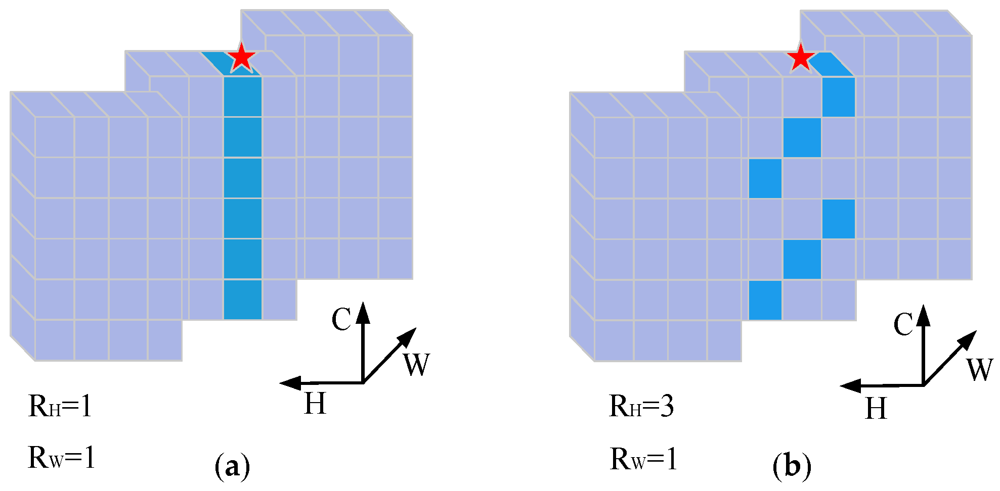[48] designed a novel variant of channel MLP named CycleMLP. The Cycle FC (fully-connected layer) in CycleMLP extracts features from different channels. Though the Cycle FC is a variant of CMLP, it has a larger spatial receptive field, even a global spatial receptive field. In low-level tasks, Tu et al. [49] solved the fixed-size problem by designing a novel spatial-gated MLP, but the model is large. Some works [46,48] have demonstrated that the CMLP framework can effectively extract global and local features and has a tradeoff between accuracy and computation cost. However, they are designed for natural images and ignore the intrinsic spectral correlation of HSIs. For the SHISR technique, SHISR can exploit the CMLP to enhance the spatial resolution while preserving the spectral information. To the best of our knowledge, there is no research on MLP in SHISR applications.

Though many CNN-based and nonlocal attention-based works have achieved good results for SHISR, there are still some problems: (1) Most works focus on local spectral features and neglect long-range spectral features. They do not sufficiently preserve the spectral information to obtain better SR performance. To alleviate spectral distortion, it is more appropriate to sufficiently extract the local and long-range spectral features. (2) Most SHISR works utilize 3D convolutions and the self-attention mechanism to extract spectral-spatial features. Because HSIs have many bands, they usually require high computation to extract the features. The SHISR methods need to better reconstruct the hyperspectral images with low computation complexity.

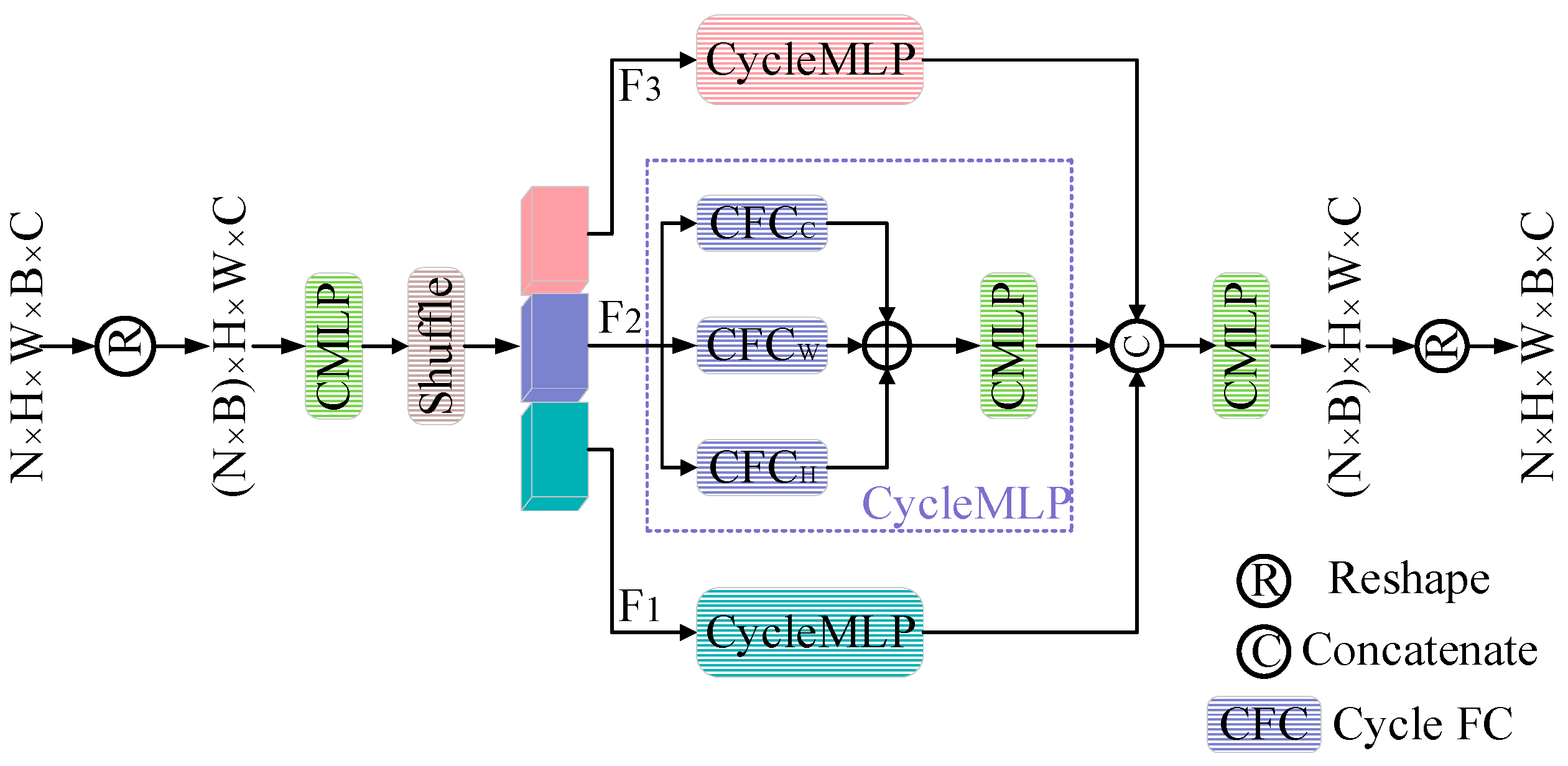
To address the above drawbacks, a spectral-spatial MLP network (SSMN) is proposed for SHISR. Considering that previous works usually reconstruct HSIs using high computation cost, our network aims to apply CMLP to obtain better reconstruction performance while reducing computation cost. Specifically, to sufficiently capture the spectral correlation, a local-global spectral integration block (LGSIB) is proposed. The LGSIB consists of CMLP and band group, band shift, and band shuffle operations, and it aims to capture the local and global spectral correlation and reduce computation complexity. Because the spatial receptive field of CMLP is limited, a spatial feature group extraction block (SFGEB) is designed. SFGEB consists of CycleMLP and a group mechanism, which aims to extract spatial features well while reducing computation complexity and the number of parameters. On the one hand, compared with CMLP, the SFGEB has a larger spatial receptive field, so it can extract more spatial features. On the other hand, compared with the convolution and self-attention mechanism, the computation complexity and number of parameters of SFGEB remain unchanged while the spatial receptive field expands.

In summary, the main contributions of this work are provided as follows:

• A novel network named SSMN that is based on CMLP is proposed for SHISR. The proposed MLP-based network can handle HSIs of different sizes. The experimental results demonstrate that our network achieves better reconstruction performance compared with other methods based on convolution and nonlocal attention.
• An LGSIB is proposed to extract rich spectral features while reducing the computation complexity; it aims to use the CMLP to extract the local spectral features using group and shift manners, and it extracts the long-range spectral features using group and shuffle manners.
• In order to extract spatial features well while maintaining computation efficiency, an SFGEB is designed, which consists of CycleMLP and a group manner; its number of parameters and computation complexity do not increase as the spatial receptive field expands.

The rest of this paper is divided into three sections. In Section 2, the proposed SSMN is introduced. In Section 3, the experiments and the results are shown. The conclusion is provided in Section 4.

2. Proposed Method

In this section, the overall network architecture is firstly introduced. Secondly, the details of the LGSIB are given. Thirdly, the SFGEB is described in detail.

2.1. Overall Network Architecture

This section will introduce the overall network architecture. As shown in Figure 1, we first apply one CMLP to extract the shallow features of LR HSIs. Then, several spectral-spatial MLP (SSMLP) blocks are used to extract complex spectral-spatial features. In one SSMLP, the local-global spectral features are captured by the LGSIB, and the spatial features are captured by the SFGEB. Next, the outputs of different SSMLP blocks are fused. Finally, the super-resolution image is reconstructed by upsampling and global residual learning.

Let $I_{\mathrm{LR}}\in {ℝ}^{H\times W\times B\times 1}$ be a low-resolution hyperspectral image, where 1, B, H, and W sequentially denote the channel dimension, number of bands, height, and width in HSIs. To preserve the structural features of HSIs, the feature map is treated as a four-dimensional cube. The goal is to reconstruct a high-resolution image $I_{\mathrm{SR}}\in {ℝ}^{(Hr)\times (Wr)\times B\times 1}$ from the I_LR image, where r is the scale factor. First, one CMLP matrix is used to linearly project the I_LR,

$$F_0=I_{\mathrm{LR}}\cdot M,$$

(1)

where $M\in {ℝ}^{1\times C}$ and $F_0\in {ℝ}^{H\times W\times B\times C}$; C denotes the channel dimension.

Next, the F₀ is fed into the SSMLP block. The SSMLP block consists of the LGSIB, SFGEB, feed-forward network (FFN), and dropout layer. The FFN is made up of two cascading CMLPs, the layer normalization, and the drop-out layer. The spectral correlation and spatial details are captured by the LGSIB and SFGEB in each SSMLP block, respectively. By separately capturing the spatial and spectral features, the number of parameters and computation complexity are reduced. We will provide more details about the LGSIB and SFGEB blocks in the following two subsections. There are several SSMLP blocks for feature learning, and the output of the previous SSMLP block is the input of the next SSMLP block. The process of extracting spectral-spatial features in one SSMLP can be formulated as:

$$\begin{array}{c}{H}_{\mathrm{n}}={\mathrm{SFGEB}}_{\mathrm{n}}({\mathrm{LGSIB}}_{\mathrm{n}}(F_{\mathrm{n}-1})+F_{\mathrm{n}-1})+F_{\mathrm{n}-1}\\ F_{\mathrm{n}}={\mathrm{FFN}}_{\mathrm{n}}(H_{\mathrm{n}})+H_{\mathrm{n}}\end{array},$$

(2)

where LGSIB_n, SFGEB_n, and FFN_n represent the blocks in the n-th SSMLP module and F_n−1 represents the output of the previous SSMLP block. Then, we fuse the outputs of all SSMLP blocks, and obtain the output F. Finally, the super-resolution image I_SR is reconstructed, and the super-resolution process can be expressed as follows:

$$I_{\mathrm{SR}}=f_{\mathrm{up}}(F)+f_{\mathrm{bicubic}}(I_{\mathrm{LR}}),$$

(3)

where $f_{\mathrm{up}}(\cdot )$ is an upsampling layer made up of three CMLPs and a pixel shuffle operation and $f_{\mathrm{bicubic}}(\cdot )$ denotes a bicubic interpolation function.

Transposed convolution is widely used for image super-resolution, but it will result in the checkerboard problem. Shi et al. [50] avoided this problem by rearranging the pixels among channels to enlarge the spatial size. To avoid the checkerboard problem, we combine CMLP with pixel rearrangement [50] to upsample the images. As shown in Figure 1, there are three CMLPs and a pixel shuffle operation in the upsample layer. The HSIs are upsampled in a band-by-band manner. Specifically, for a given band $F_{\mathrm{k}}\in {ℝ}^{H\times W\times C}$, $k\in \{1,\dots ,B\}$, the first CMLP is utilized to increase the number of channels from C to Cr². The pixel shuffle operation is applied to rearrange the pixels from the channel dimension into the spatial domain and obtain $F_{\mathrm{k}}\in {ℝ}^{(Hr)\times (Wr)\times C}$. The second CMLP is used to decrease the number of channels from C into 1. One reconstructed band $I_{\mathrm{k}}\in {ℝ}^{(Hr)\times (Wr)\times 1}$ is obtained after the upsampling. Then, we concatenate all reconstructed bands and obtain $I_{up}\in {ℝ}^{(Hr)\times (Wr)\times B\times 1}$. Because the HSIs are upsampled in a band-by-band manner, it ignores the spectral correlation among bands. To alleviate spectral distortion, the third CMLP is utilized to refine the image along spectral dimension. The final output $I_{\mathrm{SR}}\in {ℝ}^{(Hr)\times (Wr)\times B\times 1}$ can be obtained by summing the I_up and $I_{\mathrm{bicubic}}\in {ℝ}^{(Hr)\times (Wr)\times B\times 1}$.

2.2. Local-Global Spectral Integration Block

The previous works insufficiently extract the spectral features. It is more beneficial to sufficiently extract local and long-range spectral features. In addition, because of the many bands in HSIs, much computation is needed to extract the spectral features. To solve these problems, a local and global spectral integration block (LGSIB) is designed. Within the LGSIB, the group-shift-shuffle MLP block (GSSMB) is the core, which can extract the local and long-range spectral features using the CMLP. Some parameter-free operations in the GSSMB, including the band group, band shift, and band shuffle operations, are utilized to improve the feature extraction and reduce the computational complexity.

Firstly, a very simple way to extract the spectral features using CMLP is introduced. The given input $F\in {ℝ}^{H\times W\times B\times C}$ is reshaped into the size of $HW\times BC$. One CMLP matrix $M\in {ℝ}^{BC\times BC}$ is utilized to extract the spectral features along the $(BC)$ dimension. There are C feature maps in F, and many feature maps are similar [51]. To take the similarity among the feature maps and correlation among the bands, the spectral correlation is captured along the $(BC)$ dimension instead of the band dimension. The number of parameters is ${(CB)}^2$. There are many feature maps and bands, so the model is large. To alleviate the limitations, we need a strategy to reduce the number of parameters as well as the computation complexity.

The feature maps are redundant [52], which indicates that it is possible to extract features from redundant feature maps with low computation cost. Therefore, the feature maps are split into two groups in the LGSIB, and only one cheap CMLP is used to linearly project one group along the channel dimension; meanwhile, one GSSMB is used to extract complex spectral features from the other group. Specifically, the input $F\in {ℝ}^{H\times W\times B\times C}$ is firstly projected along the channel dimension, which is then split into two groups:$F_1\in {ℝ}^{H\times W\times B\times \alpha C}$ and $F_2\in {ℝ}^{H\times W\times B\times (1-\alpha )C}$, $\alpha \in [0,1]$. We set $\alpha =1/2$ in our experiments so that both F₁ and F₂ $\in {ℝ}^{H\times W\times B\times c}$, $c=C/2$. In particular, F₁ is treated as the redundant feature maps. Only one cheap CMLP matrix $M\in {ℝ}^{c\times c}$ is used to project F₁, while the GSSMB is used to extract the complex spectral features from F₂. Because the redundancy of the feature maps is exploited, the computation cost and number of parameters are reduced. We will provide more details about the GSSMB, which is used to further lessen the number of parameters and computation cost. Finally, we fuse two outputs and obtain $F_3\in {ℝ}^{H\times W\times B\times C}$.

As shown in Figure 2, there are three blocks in the GSSMB: the local spectral integration block (LSIB), shift spectral integration block (SSIB), and global spectral integration block (GSIB). The LSIB and SSIB aim to extract two kinds of local spectral features and complement each other. The GSIB aims to extract the global spectral features. In addition, there are three kinds of parameter-free operations in GSSMB, including the band group, band shift, and band shuffle operations. They are used to split the feature maps, shift the bands, and rearrange the bands. The combination of CMLP and parameter-free operations can improve feature extraction. Three blocks and operations will be introduced one-by-one.

The LSIB aims to extract local spectral features in a group-by-group manner. Specifically, the input $F_2\in {ℝ}^{H\times W\times B\times c}$ is firstly reshaped into $HW\times B\times c$, then split into D groups along band dimension. Each group $X^{\mathrm{d}}\in {ℝ}^{HW\times T\times c}$ contains T bands, $d\in \{1,\cdots ,D\}$ and $B=D\cdot T$. All X^d are fed into the LSIB. Each group is reshaped into $X^{\mathrm{d}}\in {ℝ}^{HW\times Tc}$, and one CMLP is applied to extract the spectral features of a group:

$$O_{\mathrm{d}}=X^{\mathrm{d}}\cdot M_{\mathrm{d}},$$

(4)

where $M_{\mathrm{d}}\in {ℝ}^{Tc\times Tc}$ and $O_{\mathrm{d}}\in {ℝ}^{HW\times Tc}$. Because the feature maps are split into groups along the band dimension, the adjacent bands are grouped into a group so that the local spectral correlation can be captured. The number of parameters of one group is ${(cT)}^2$, and there are D groups in X; thus, the number of parameters of all groups is $D\cdot {(cT)}^2$. The number of parameters is further reduced from ${(CB)}^2$ to ${(cT)}^2$ instead of $D\cdot {(cT)}^2$ by sharing the weights of M_d in the Equation (4). Finally, each group $O_{\mathrm{d}}\in {ℝ}^{HW\times Tc}$ is reshaped to the original size, and we obtain the output $O\in {ℝ}^{H\times W\times B\times c}$.

The LSIB groups the feature maps along the band dimension, and the adjacent bands are split into the same group. Thus, local spectral correlation can be captured. The number of parameters and the computational cost are reduced. However, owing to different hyperspectral sensors with different characteristics, different HSIs have different spectral correlation. The fixed group in the LSIB is not suitable for different HSI datasets. To solve this problem, the SSIB is designed to extract complementary spectral features for the LSIB. As the LSIB ignores the connections among adjacent groups, the SSIB aims to obtain those connections. In the SSIB, there are several CMLPs and a band shift operation. Specifically, the band shift operation is firstly used to shift s bands for F₂ along the band dimension. Figure 2 provides an example of shifting one band. After shifting, the feature maps are also grouped along the band dimension. All groups are then extracted by several CMLPs. In the SSIB, the next feature extraction process is the same as that of the LSIB. With the shift and group operations, the connection among adjacent groups is obtained in the SSIB. Finally, the bands are shifted back to their original order. Similar to the LSIB, the SSIB also extracts the local spectral features. The LSIB and SSIB can complement each other because they extract local but different spectral features. After fusing the outputs of the LSIB and SSIB, the network can be more suitable for different HSIs.

The LSIB and SSIB only capture the local spectral correlation and ignore the long-range spectral correlation; they are insufficient for preserving the spectral information. For spectral preservation, it is more appropriate for sufficiently extracting local and long-range spectral features. Previous works have extracted the long-range spectral features with much computation cost. To obtain the long-range spectral correlation with low computational cost, we designed the GSIB. In the GSIB, there are several CMLPs and a band shuffle operation. The band shuffle operation is firstly used to rearrange the bands, and several CMLPs are used to extract the long-range spectral features in a group-by-group manner. After fusing the two outputs from LSIB and SSIB, a feature map $Z\in {ℝ}^{H\times W\times B\times c}$ is obtained, and it is reshaped into the size $HW\times B\times c$. We shall now provide more details about the band shuffle operation. Specifically, the new feature map Z is grouped into D groups along the band dimension and obtain $Z_1\in {ℝ}^{HW\times (D\times T)\times c}$. Then, Z₁ is transposed into $Z_2\in {ℝ}^{HW\times (T\times D)\times c}$. Next, Z₂ is flattened back to the original size $Z_3\in {ℝ}^{HW\times B\times c}$. After flattening, the bands in the feature map Z₃ are shuffled. The originally long-range bands now become adjacent bands. To extract the long-range spectral features with low computational cost, Z₃ is split into D groups again. Each group contains T bands. We set D and T as 2 and 3, respectively, as an example in Figure 2. All groups will be extracted by several CMLPs. The following feature extraction process of the GSIB is the same as that of the LSIB. Finally, the bands are rearranged back to the original order. The long-range bands are split into the same group using the shuffle and group operations so that the long-range spectral correlation can be captured. The number of parameters in the GSIB is ${(cT)}^2$, which is much less than ${(CB)}^2$.

Because of the group, shift, and shuffle operations in the LGSIB, the local-global spectral features can be sufficiently captured, and the number of parameters and computation cost are reduced. In particular, the number of parameters is reduced from ${(CB)}^2$ to $\frac{1}{4}{C}^2(3T^2+11)$, and the computational complexity is reduced from $HW{C}^2{B}^2$ to $\frac{1}{4}HW{C}^2(3T^2+11)$.

2.3. Spatial Feature Group Extraction Block

The weight parameters of spatial MLP are configured by the image size. Therefore, the methods [43,44,45] based on spatial MLP need a fixed-size input during training and inference modes. For the SHISR technique, it is necessary to design a model to deal with various image sizes. In addition, previous works [31,32,41,42] have usually utilized many convolutions or self-attention mechanisms to capture the spatial details with high computation complexity, and their computation complexity increases as the spatial receptive field expands.

To extract spatial features well with low computational cost, a spatial feature group extraction block (SFGEB) is designed, which consists of CycleMLP and a group mechanism. Because of the limited spatial receptive field of CMLP, CycleMLP is utilized to extract spatial features. Similar to CMLP, CycleMLP can deal with flexible image sizes. The Cycle FC (fully-connected layer) in CycleMLP expands the receptive field of CMLP while keeping the same computation complexity and number of parameters as that of CMLP. To further reduce the computational complexity, the feature maps are split into K groups along channel dimension, and K CycleMLPs are used to extract spatial features from K groups.

The details about the Cycle FC shall be provided. Mathematically, the $F\in {ℝ}^{H\times W\times C_{in}}$ denotes an input. As shown in Figure 3, the channel FC extracts spatial features on the same position along the channel dimension; however, the Cycle FC can capture the relationship among patches on neighbor channels. The definition of the Cycle FC can be described as follows:

$$\mathrm{Cycle} \mathrm{FC}{(F)}_{i,j,:}={\displaystyle \sum _{c=0}^{C_{in}}{F}_{i+{\delta }_i(c),j+{\delta }_j(c),c}}\cdot M_{c,:}^{mlp}+b,$$

(5)

where $M^{mlp}\in {ℝ}^{C_{in}\times C_{out}}$ and $b\in {ℝ}^{C_{out}}$. The parameters ${\delta }_i(c)$ and ${\delta }_j(c)$ mean the offset along the height and width on the c-th channel, and their definition can be formulated as follows:

$${\delta }_i(c)=(c \mathrm{mod} R_{\mathrm{H}})-1, {\delta }_j(c)=(⌊\frac{c}{R_{\mathrm{H}}}⌋\mathrm{mod} R_{\mathrm{W}})-1,$$

(6)

where R_H and R_W are the step size along the height and width. The Cycle FC in CycleMLP introduces a larger receptive field (R_H, R_W) compared with CMLP. We set R_H and R_W to 3 and 1, respectively, as an example in Figure 3b.

The Cycle FC can extract features from different positions in a cyclical extraction approach. Therefore, the Cycle FC can extract the spatial features from a larger spatial range and even from a global spatial receptive field. The CycleMLP consists of three parallel Cycle FCs and one CMLP,

$$\mathrm{CycleMLP}=\mathrm{CMLP}(\mathrm{Cycle}{\mathrm{FC}}_{\mathrm{H}}(F)+\mathrm{Cycle}{\mathrm{FC}}_{\mathrm{W}}(F)+\mathrm{Cycle}{\mathrm{FC}}_{\mathrm{C}}(F)),$$

(7)

where F denotes the input and Cycle FC_H, Cycle FC_W, and Cycle FC_C are the applied Cycle FC along the height, width, and channel dimensions, respectively.

More details about the SFGEB are provided in Figure 4. The input $F\in {ℝ}^{N\times H\times W\times B\times C}$ is firstly reshaped into the size of $(N\times B)\times H\times W\times C$. The spatial features are extracted in a band-by-band manner in the SFGEB. Because it is beneficial to extract spatial features by interacting with the information along the channel dimension, the channels of the feature maps are shuffled. Next, the SFGEB is extended into a multiple branch style to reduce the computation cost. As shown in Figure 4, the feature maps are split into K groups $\{F_1,F_2,\dots ,F_K\}$ along the channel dimension, and each group is fed into one CycleMLP. The outputs of each branch are concatenated, and one CMLP is used to fuse them. Finally, the output $O\in {ℝ}^{N\times H\times W\times B\times C}$ is obtained.

Because of the Cycle FC in the SFGEB, the number of parameters and computation complexity do not increase as the spatial receptive field expands. Compared with CMLP, the spatial receptive field of SFGEB is larger. Compared with spatial MLP, whose computation complexity is quadratic to the image size, SFGMB has a linear complexity. Thus, the SFGEB can sufficiently extract spatial features while reducing the computation complexity. In addition, the feature maps are grouped in the SFGEB, meaning that the computational cost can be further reduced.

3. Experiments and Results

In this section, we will verify the performance of the proposed model according to the quantitative and qualitative results. Firstly, four common public hyperspectral remote sensing datasets are considered, and the implementation details are provided. Next, the evaluation metrics and comparison methods are introduced. Then, the ablation experiments are conducted to demonstrate the effectiveness of our network blocks. Finally, the proposed method is compared with state-of-the-arts algorithms.

3.1. Datasets and Implementation Details

3.1.1. Datasets

• Houston Dataset: The Houston dataset [53] was acquired by a remote sensor ITRES CASI 1500 and was released by the National Center for Airborne Laser Mapping at the University of Houston in 2018. It covers a 380–1050 nm spectral range and contains 48 bands. The image size is 4172 × 1202. We divide it into a training region and testing region at a ratio of seven to three. In addition, the training region is flipped horizontally, rotated (90°, 180°, 270°), and cut into 9180 training reference images with a size of 48 × 48 × 48 each. The test region is randomly cut into 16 non-overlapping testing reference images, and their sizes are all 144 × 144 × 48.
• Chikusei Dataset: The Chikusei hyperspectral dataset [54] was taken by the Headwall Hyperspec-VNIR-C imaging sensor over agricultural and urban areas in Chikusei, Ibaraki, Japan, in 2014. It covers a spectral range from 363 nm to 1018 nm and contains 128 bands. The image size is 2517 × 2335, and the spatial resolution is 2.5 m. The dataset is divided into two parts: a training region for 70% of the dataset and a test region for 30% of the dataset. The training region is cut into 7872 training reference images, and each sample has a size of 48 × 48 × 128. The test region is randomly cut into 14 non-overlapping testing reference images with the size of 144 × 144 × 128.
• HSRS-SC Dataset: This dataset [55] was collected by a compact airborne spectrographic imager (CASI). There are 1385 hyperspectral remote sensing images, which are classified into five types of scenes. Each scene contains 154–485 images. Each image consists of 48 bands, which covers a spectral range from 380 nm to 1050 nm. The size of each image is 256 × 256 × 48. We choose 500 images from the 5 scenes and cut 7980 training images with the size of 48 × 48 × 48 each. Ten images are randomly selected from the five types of scenes for testing images, and their top left regions are cut into the testing reference images at a size of 144 × 144 × 48.
• Washington DC Mall Dataset: This dataset [56] was acquired by a hyperspectral digital image collection experiment (HYDICE); it covers a spectral range from 400 nm to 2400 nm and contains 191 bands. The spatial resolution is 3 m, and the image size is 1280 × 307. We divide the data into two parts: a training region for 70% of the dataset and a testing region for 30% of the dataset. The training region is cut into 7800 reference samples. The size of each training reference image is 48 × 48 × 191. The testing region is split into six testing reference images with a size of 144 × 144 × 191.

The above training images with a size of 48 × 48 are the HR reference images, while the LR training images are generated by a Gaussian point spread function and downsampling of the reference images with three scale factors, i.e., 2, 3, and 4. Because we conduct the experiments with scale factor ×2, ×3, and ×4, the size of 48 × 48 can be divisible by 2, 3 and 4. The size of 48 × 48 is also widely set in SR methods [21,57]. The test image with the size of 144 × 144 is the reference image, while the LR test image is generated by a Gaussian point spread function and by downsampling the reference image with three scale factors. The specific size of 144 × 144 can be divisible by a scale factor of 2, 3 and 4, which was used in [58]. Because our network is made up of CMLP, the weight parameters are not related to the height and width. Thus, our method can handle HSIs of any size in the inference phase. We do not super-resolve test images with a larger size, due to the huge memory requirement of HSIs.

3.1.2. Implementation Details

There are many kinds of loss functions [59,60,61]. The l₁ and l₂ loss functions are widely used in SHISR. The l₂ loss penalizes larger errors compared with the l₁ loss, and the l₁ loss has a better convergence performance [21,62,63]. In addition, when the final loss function contains multiple losses, it is difficult to control the balance factor to obtain better performance. Thus, the l₁ loss function was chosen to train the super-resolution network. An ablation experiment was conducted to prove that our method obtains a better performance with the l₁ loss instead of the l₂ loss.

The adaptive moment estimation optimizer (ADAM) (${\beta }_1=0.9$, ${\beta }_2=0.999$) is used. The initial learning rate is 0.0002 and is halved every 35 epochs. The dropout rate is 0.1, and the batch size is 16. The number of the SSMLP blocks is four. The number of channels is set to 64 for all SSMLP blocks. In the SSIB, we shift three bands for all datasets. In the SSIB and LSIB, we split the feature maps into six groups for the Houston and HSRS-SC datasets, eight groups for the Chikusei dataset, and sixteen groups for the Washington DC Mall dataset. In the GSIB, we split the feature maps into eight groups for the Houston and HSRS-SC datasets, six groups for the Chikusei dataset, and twelve groups for the Washington DC Mall dataset. When the number of bands is not divisible by the group number, the related bands are used for padding. In the SFGEB, the number of branches K is four. We set (R_H, R_W) as (5, 1), (1, 5), (1, 1) for three Cycle FCs in the CycleMLP. All experiments were conducted on one NVIDIA GTX 1080Ti GPU using the Pytorch framework. The code is released at https://github.com/corkiyao/SSMLP (accessed on 8 June 2023).

3.2. Evaluation Metrics and Comparison Methods

3.2.1. Evaluation Metrics

To evaluate the performance of super-resolution algorithms, three widely used evaluation metrics were used, including the mean peak signal-to-noise ratio (MPSNR), mean structure similarity (MSSIM), and spectral angle mapper (SAM). The MPSNR evaluates the similarity based on the mean squared error (MSE) between the reference image and the reconstructed image. The MSSIM is used to measure the mean structural similarity between the reference image and the reconstructed image. Larger MPSNR and MSSIM values indicate a better visual quality of the reconstructed SR images. The SAM [64] evaluates the spectral fidelity between the reference image and the reconstructed image, and a smaller SAM indicates better spectral preservation. In addition, floating point operations (FLOPs) were used to evaluate the model complexity. It is usually calculated using the number of multiplication and addition operations that a network performs. In our experiments, the FLOPs metric is calculated when a network processes one image in the inference phase. The larger the FLOPs value, the higher the computation cost.

3.2.2. Comparison Methods

In order to demonstrate the performance of the proposed network, our method is compared with seven super-resolution methods: bicubic, VDSR [20], 3DFCNN [28], EDSR [21], gradient-guided residual dense network (GRDN) [25], HLNnet [40], and Interactformer [41]. The bicubic method is the classical interpolation. The VDSR and EDSR are representatives of CNN-based natural image super-resolution methods. For the hyperspectral super-resolution, we apply the VDSR and EDSR networks in a band-by-band manner. The 3DFCNN, GRDN, Interactformer, and HLNnet methods are classical and recent SHISR methods that are based on deep learning. We carefully set the hyper-parameters to obtain the best performance of the compared methods.

3.3. Ablation Study

In this section, we verify the effectiveness of the proposed method by conducting experiments on the Houston dataset with a scale factor of four. The bold text of the evaluation metrics represents the best results of ablation experiments.

First, the experiments on the number of SSMLP blocks are conducted.

Table 1. Ablation study of the number of SSMLP blocks in the Houston dataset (scale factor 4).

	2	3	4	5
MPSNR	30.70739	30.86136	31.10764	31.01103
MSSIM	0.98126	0.98190	0.98286	0.98230
SAM	1.96019	1.93722	1.93722	1.87152

provides the evaluation index of two, three, four, and five SSMLP blocks. From Table 1, we can see that our network performs best when the number of SSMLP blocks is four. Due to the limitation of model capability, a shallow network is difficult to obtain a good reconstruction performance. The results indicate that a deeper network can achieve better results. It can be seen that when the evaluation index is larger, the results are better. However, the performance slightly decreases when the number of SSMLP blocks is five. Because more SSMLP blocks contain a larger number of parameters, it is difficult to train a larger network. In addition, the network with more parameters easily results in overfitting. Therefore, the number of SSMLP blocks is set as four in our network.

Some ablation experiments were conducted to verify the effectiveness of the proposed LGSIB and SFGEB in the SSMLP block. To verify the capability of the LGSIB and SFGEB, one of them was separately removed. The results are shown in

Table 2. Ablation study of the network structures in the Houston dataset (scale factor 4).

	Remove LGSIB	Remove SFGEB	Ours (LGSIB + SFGEB)
MPSNR	30.12244	28.35876	31.10764
MSSIM	0.97797	0.96713	0.98286
SAM	2.21080	2.55483	1.86055
FLOPs/Params	20 G/167 K	30 G/713 K	36 G/773 K

. First, the LGSIB is removed and the SFGEB is kept. It is observed that the SR performance greatly decreases after removing the LGSIB. When the LGSIB is removed, the SAM is larger than that of our method. Thus, these results demonstrate that the proposed LGSIB can effectively extract spectral features. Second, the SFGEB is removed while keeping the LGSIB. We can see that the SR performance greatly decreases after removing the SFGEB. Compared with our method, when the SFGEB is removed, the MPSNR and MSSIM are smaller and the SAM is larger. Thus, the network without the SFGEB can hardly extract spatial features. It proves the benefit of the SFGEB. The above experiments prove that both the LGSIB and SFGEB are beneficial for HSI super-resolution.

Then, to verify the effect of the group manner in GSSMB, some experiments on different numbers of groups were conducted. The results are shown in

Table 3. Ablation study of the group strategy in the GSSMB in the Houston dataset (scale factor 4).

	MPSNR	MSSIM	SAM	FLOPs/Parmas
D = 16, T = 3	30.81104	0.98160	1.91978	37 G/1337 K
D = 12, T = 4	30.84086	0.98178	1.91453	36.5 G/935 K
D = 8, T = 6	31.10764	0.98286	1.86055	36 G/773 K
D = 6, T = 8	30.82077	0.98150	1.93260	36 G/886 K
D = 4, T = 12	30.75321	0.98104	1.92677	38 G/1461 K
D = 3, T = 16	30.75807	0.98138	1.94952	44 G/2350 K
Without Group	30.84261	0.98167	1.89772	100 G/28,000 K

. It is observed that the number of parameters is large and the computational cost is high when the group strategy is removed. Compared with methods using the group strategy, the GSSMB without the group manner does not obtain a better performance. We consider that it is difficult to train the GSSMB with so many parameters, and the limited performance is possibly caused by overfitting. Therefore, the group manner can reduce the parameters to avoid the overfitting problem and allow the model to be easily trained. Moreover, it can be found that our method with the group manner obtains the best performance when the number of D is eight. Because of the redundancy of spectral information, when the number of D increases from three to eight, the negative effect of redundancy is gradually reduced. However, the results become worse when the number of D is larger than eight. Because the bands are consecutive, it will cause inconsistent estimation when there are many groups. In addition, it is very complex to be constantly adjusting the number of D to obtain better performance for different HSIs datasets. Therefore, to obtain good performance with less computational cost, the numbers of D and T are designed to reduce the FLOPs as much as possible for other HSIs.

Some ablation experiments were further conducted to verify the effects of three blocks in the GSSMB: the LSIB, SSIB, and GSIB. The results are shown in

Table 4. Ablation study of the GSSMB structures in the Houston dataset (scale factor 4).

LSIB	SSIB	GISB	MPSNR	MSSIM	SAM	FLOPs/Params
×	√	√	30.88751	0.98204	1.92179	32 G/621 K
√	×	√	30.93368	0.98199	1.90345	32 G/621 K
√	√	×	31.00853	0.98238	1.87792	30 G/510 K
√	√	√	31.10764	0.98286	1.86055	36 G/773 K

. After removing one of three blocks, the evaluation metrics are worse. When one of the LSIB and SSIB blocks is removed, the results become worse, which proves that each of them has a positive effect on improving the reconstruction performance and that they can complement each other. We find that after removing the GSIB, the MPSNR drops. It indicates that the GSIB can improve super-resolution performance by capturing long-range spectral features.

Next, we investigated the effects on the number of branches K in SFGEB. The results are shown in

Table 5. Ablation study of the number of branches in the SFGEB in the Houston dataset (scale factor 4).

	K = 1	K = 2	K = 4	K = 8
MPSNR	30.94025	30.96333	31.10764	30.91139
MSSIM	0.98216	0.98215	0.98286	0.98207
SAM	1.90974	1.88769	1.86055	1.92063
FLOPs/Params	42 G/847 K	38 G/798 K	36 G/773 K	34 G/761 K

. It is observed that our network obtains the best performance when the number of K is set to four. As the number K increases from one to four, the results become better and the FLOPs decreases. It is easier to train the SFGMB with less parameters. When the number of K is eight, the MPSNR slightly decreases. Because the input channels for each CycleMLP become fewer, it may the harm representation capability. Therefore, to balance the reconstruction performance and computational cost, the number of K in the SFGEB is set to four for all HSIs datasets.

Finally, we would like to report the effect of the l₁ and l₂ loss functions, which are commonly used to train super-resolution networks. The quantitative comparisons are shown in

Table 6. Ablation study of the loss function in the Houston dataset (scale factor 4).

	l1	l2
MPSNR	31.10764	30.92505
MSSIM	0.98286	0.98218
SAM	1.86055	1.90519

. It is found that our method obtains a better reconstruction performance when using the l₁ loss function. The l₁ loss function does not penalize larger errors and has better convergence compared with the l₂ loss function [21,62,63]. Thus, the l₁ norm is chosen to train our network.

3.4. HSI SR Experiments and Results

In this section, we show the experimental results on the Houston, HSRS-SC, Chikusei, and Washington DC Mall datasets. The experiments were conducted with three scale factors, i.e., ×2, ×3, and ×4. The qualitative and quantitative results are analyzed. The red and blue text of the quantitative evaluation metrics represent the best and second best results, respectively.

3.4.1. Results of Houston Dataset

The quantitative results of the Houston dataset are shown in

Table 7. Quantitative comparison of the Houston dataset. The red and blue text indicate the best and second best result values, respectively.

Scale	Metrics	Bicubic	VDSR	3DFCNN	EDSR	GRDN	HLNnet	Interactformer	Ours
×2	MPSNR	33.61036	36.81006	36.31081	36.90783	37.39292	37.31068	37.41921	37.63251
	MSSIM	0.99014	0.99544	0.99500	0.99559	0.99604	0.99602	0.99609	0.99634
	SAM	1.43970	1.12807	1.20455	1.08717	1.042401	1.04733	1.03844	1.00473
×3	MPSNR	30.33877	32.88569	32.38918	32.93509	33.37765	33.27358	33.47990	34.22439
	MSSIM	0.97854	0.98837	0.98723	0.98865	0.98967	0.98952	0.98991	0.99180
	SAM	2.03853	1.69531	1.73596	1.64159	1.57840	1.57629	1.55615	1.39556
×4	MPSNR	27.82178	30.03148	29.53820	29.98065	30.32926	30.41107	30.50146	31.10764
	MSSIM	0.96086	0.97711	0.97493	0.97736	0.97874	0.97935	0.97947	0.98286
	SAM	2.73205	2.30920	2.34192	2.24042	2.18900	2.15620	2.13343	1.86055

. It is observed that our method is better than other methods in the literature. For example, when the scale factor is four, the MPSNR of our method is 0.6 dB higher than that of Interactformer, and the SAM of our method is 0.27 lower than that of Interactformer. Because VDSR and EDSR ignore the protection of spectral information, their results are worse than the results of the other algorithms, except for bicubic and 3DFCNN. The evaluation metrics of 3DFCNN are worse than that of VDSR and EDSR. The main reasons are that the 3DFCNN network is shallow; furthermore, there is no residual learning in the 3DFCNN network. Compared with VDSR and EDSR, GRDN achieves a better performance. GRDN can extract extra spatial gradient details, while the VDSR and EDSR ignore that factor. Interactformer obtains the second best performance by combining the CNN with the transformer to capture the local and global dependencies. In addition, compared with the other methods, the superiority of the SAM of our methods gradually increases when the scale factor becomes larger. There are two main reasons for this. The first is that it is more difficult to super-resolve HSIs as the scale factor grows. The second is that the other methods lack sufficient spectral features learning. Because we propose the LGSIB to sufficiently capture the local and global spectral features, our method can alleviate the problem. 3DFCNN and Interactformer only extract local spectral features. HLNnet only utilizes one nonlocal attention block to extract the long-range spectral features in the first model layer, while the other layers are still used for local spectral features learning.

The above quantitative analysis is also supported by the reconstructed images, which are shown in Figure 5. To show more details, an area marked by the red rectangle is enlarged from the ground truth image as a reference. The same region marked by the red rectangle from the reconstructed images of each method is also enlarged. As shown in Figure 5, our method produces sharper edges, as is the case for the edge of the center building; for HLNnet and Interactfomer, artifacts appear, and EDSR and VDSR produce blurry results. This result proves that our network can better reconstruct super-resolution images. To further validate the effectiveness of our methods, we also provide the error images between the super-resolution images and the reference images shown in Figure 6. When the error image is bluer, it means that the super-resolution image is closer to the reference image. The visualization results indicate that the error map of our method is the bluest. Our reconstructed image is the closest to the ground truth image.

3.4.2. Results of the HSRS-SC Dataset

The experiments were also conducted on the HSRS-SC dataset. The quantitative results are shown in

Table 8. Quantitative comparison of the HSRS-SC dataset. The red and blue text indicate the best and second best result values, respectively.

Scale	Metrics	Bicubic	VDSR	3DFCNN	EDSR	GRDN	Interactformer	HLNnet	Ours
×2	MPSNR	30.91831	34.05928	33.47056	33.93229	34.21800	34.80833	35.39844	35.65883
	MSSIM	0.94983	0.97460	0.97133	0.97399	0.97520	0.97776	0.98000	0.98116
	SAM	2.97044	2.52064	2.63652	2.5332	2.50794	2.43484	2.41159	2.31576
×3	MPSNR	28.25784	30.30507	29.89933	30.22463	30.43345	30.73033	31.28533	31.64508
	MSSIM	0.90746	0.94316	0.93805	0.94254	0.94499	0.94814	0.95406	0.95812
	SAM	3.60363	3.21843	3.32278	3.25291	3.23010	3.15388	3.14645	3.03447
×4	MPSNR	26.43125	28.04833	27.80732	28.02282	28.27791	28.60088	28.68334	29.41301
	MSSIM	0.85667	0.90510	0.89981	0.90566	0.90980	0.91632	0.91747	0.93254
	SAM	4.15459	3.79804	3.83266	3.83179	3.75885	3.60442	3.71579	3.48209

, and the visual results are shown in Figure 7 and Figure 8. From Table 8, it can be seen that our method still obtains the best performance for the three scale factors. For instance, when the scale factor is three, the evaluation metrics of MPSNR, MSSIM and SAM in our method are better than the results of HLNnet, i.e., +0.37 dB, +0.004, and −0.11, respectively. Because VDSR and EDSR ignore the protection of spectral correlation information, their evaluation metrics are still worse than the results of our method. Compared with those of CNN-based methods (i.e., 3DFCNN, VDSR, and EDSR), Interactformer and HLNnet obtain a better performance through the combination of the local and global features. In addition, the SAM of our method is still the smallest for the three scale factors. The proposed local-global spectral integration block (LGSIB) can still sufficiently extract spectral features in the HSRS-SC dataset.

The super-resolution images on the HSRS-SC dataset are presented in Figure 7. The region marked by the red rectangle is enlarged to present more details. From Figure 7, the super-resolution image of our method is better than that of the other comparison methods. Our method can reconstruct more clear edges, as is the case for the edge of the center building, while other comparison methods produce images with artifacts or cause spectral distortion to appear. Moreover, we provide the error maps between the super-resolution images and the reference images in Figure 8. It can be seen that our error map is the bluest, which means that the super-resolution image of our method is the closest to the reference image. Thus, the proposed method obtains the best reconstruction performance on this dataset.

3.4.3. Results of the Chikusei Dataset

Some experiments were also conducted on the Chikusei dataset. In contrast to the Houston and HSRS-SC datasets, the Chikusei dataset contains more bands (up to 128). The evaluation metrics of each method are shown in

Table 9. Quantitative comparison of the Chikusei dataset. The red and blue text indicate the best and second best result values, respectively.

Scale	Metrics	Bicubic	VDSR	3DFCNN	EDSR	GRDN	HLNnet	Interactformer	Ours
×2	MPSNR	31.35162	34.66397	33.56629	35.41532	34.76920	35.65999	35.70729	36.36153
	MSSIM	0.97117	0.98690	0.98344	0.98850	0.98714	0.98916	0.98915	0.99095
	SAM	2.33774	1.86435	1.92614	1.74509	1.86396	1.66459	1.66064	1.51879
×3	MPSNR	28.74680	30.77485	30.20889	31.19459	30.66312	31.41036	31.53661	32.07586
	MSSIM	0.94507	0.96684	0.96262	0.96877	0.96589	0.96959	0.97034	0.97443
	SAM	3.13851	2.77739	2.74645	2.65812	2.81941	2.60161	2.57006	2.29185
×4	MPSNR	26.84760	28.41971	27.94085	28.70123	28.23195	29.13901	29.15101	29.51723
	MSSIM	0.91151	0.94050	0.93509	0.94331	0.93866	0.94607	0.94665	0.95208
	SAM	3.95445	3.61779	3.54112	3.47155	3.64814	3.32975	3.32009	3.01902

. Even though the number of bands increases, the evaluation metrics of our method still are the best for the three scale factors. For example, when the scale factor is four, the MPSNR, MSSIM, and SAM of our method are better than the results of Interactformer, i.e., +0.36 dB, +0.006, and −0.30, respectively. The 3DFCNN network is still worse than VDSR and EDSR because of the shallow network without residual learning. Compared with VDSR, EDSR, and GRDN, HLNnet and Interactformer still obtain better performances because they can extract local-global features and focus on preserving the spectral information. In addition, as the number of bands increases, the evaluation metric SAM of our algorithm is still smaller than that of HLNnet and Interactformer. The proposed LGSIB can still sufficiently extract the local and global spectral features to alleviate the spectral distortion. Therefore, the SAM of our method is smaller.

The super-resolution images and error images are also provided in Figure 9 and Figure 10. From Figure 9, we can find that our method can produce more details, such as the two slashes in the center, while GRDN, HLNnet, and Interactformer only produce one slash or one mutilated slash. In addition, bicubic and 3DFCNN reconstruct blurry images, and VDSR and EDSR produce images with artifacts. Furthermore, we also provide the error maps between the super-resolution images and the reference images; they are shown in Figure 10. It can be seen that our error map presents less error between the reference image and the reconstructed image. Therefore, our method obtains the best performance on the Chikusei dataset.

3.4.4. Results of the Washington DC Mall Dataset

To further prove the effectiveness of our method on a dataset with a higher number of bands, we conducted experiments on the Washington DC Mall dataset. This dataset contains more bands, numbering up to 191 bands, which means that it is more difficult to super-resolve this dataset. Three evaluation metrics for all comparison methods are shown in

Table 10. Quantitative comparison of the Washington DC Mall dataset. The red and blue text indicate the best and second best values, respectively.

Scale	Metrics	Bicubic	VDSR	3DFCNN	EDSR	GRDN	HLNnet	Interactformer	Ours
×2	MPSNR	26.31294	28.61898	28.40655	28.22535	28.82269	29.02062	29.11935	29.51473
	MSSIM	0.93673	0.96601	0.96450	0.96328	0.96810	0.96945	0.96998	0.97324
	SAM	5.33994	4.53473	4.58621	5.26906	4.84116	4.42888	4.25528	4.09366
×3	MPSNR	23.96104	24.76885	25.04055	24.89591	25.19442	25.41548	25.47882	25.81161
	MSSIM	0.88532	0.91593	0.91989	091829	0.92320	0.92764	0.92855	0.93672
	SAM	6.85189	7.40664	6.24949	7.09555	6.63486	6.37467	6.10688	5.80900
×4	MPSNR	22.40923	22.62539	23.27383	22.99236	23.45084	23.49942	23.61296	23.80055
	MSSIM	0.82603	0.85669	0.87577	0.87095	0.88010	0.88131	0.88516	0.89830
	SAM	8.12052	9.36632	7.44784	8.52248	7.65482	7.47232	7.30512	7.07873

. It can be seen that our method still performs the best in the Washington DC Mall dataset. For instance, when the scale factor is three, the MPSNR and MSSIM values are larger than that of Interactformer, i.e., +0.33 and +0.012, respectively. Because the dataset contains more bands compared with the Houston, HSRS-SC, and Chikusei datasets, it is more difficult to capture the spectral correlation. Other comparison methods (i.e., VDSR, EDSR, and GRDN) cannot sufficiently extract spectral features, which leads to spectral distortion. The SAM of our method is the smallest among all methods. The main reason is that the proposed LGSIB can sufficiently extract the local and global spectral features, which better preserves spectral information. Thus, our method obtains the best reconstruction performance despite the dataset containing a higher number of bands.

The super-resolution images are provided in Figure 11. We find that the proposed method reconstructs images with clear boundaries. EDSR, VDSR, and GRDN present spectral distortion, bicubic produces blurry results, and 3DFCNN presents artifacts. In addition, we also provide the error maps between the reconstruction images and the reference images in Figure 12. It is observed that our error map presents lower error between the SR image and the reference image. Therefore, our method still obtains the best reconstruction performance in the dataset that contains a higher number of bands.

The spectral curve can show the continuous spectra of the same location. The difference curve is obtained by calculating the spectral vector difference between the SR image and the reference image. When two spectral curves are consistent, it means that two images are very similar. When the difference curve is closer to zero, it means that the spectral vector of the SR image is closer to that of the reference image. We randomly selected pixels for the spectral curves and difference curves. The curves for the three datasets are shown in Figure 13. As shown in Figure 13, our difference curves are closer to zero. This result means that the spectral vectors of our reconstructed images are closer to that of the reference images. The spectral curves of our methods are more consistent with that of the reference images, while the spectral curves of other methods (i.e., VDSR, GRDN, EDSR, and HLNnet) are inconsistent with that of the reference images. This proves that our method can achieve a better spectral preservation compared with the other methods.

3.5. Computation Cost

In this section, to compare the computation cost of all deep learning methods, the number of parameters, inference time, MPSNR, and FLOPs are provided in

Table 11. Computation cost for all methods in the Chikusei dataset (scale factor 4).

Metrics	VDSR	3DFCNN	EDSR	GRDN	HLNnet	Interactformer	Ours
Time (s)	1.91	0.12	0.56650	0.14	0.30	0.37	0.23
FLOPs (G)	220	208	640	556	2960	2530	124
Params (K)	665	39	1515	838	9899	4642	2592
MPSNR (dB)	28.41971	27.94085	28.23195	28.70123	29.13901	29.15101	29.51723

. All methods were tested on Chikusei dataset with a scale factor of four on a GeForce GTX 1080Ti GPU using the Pytorch framework. All methods were tested 50 times, and the inference time is the average of the total time. In Table 11, because VDSR and EDSR super-resolve the HSIs in a band-by-band manner, their inference time are longer than other methods. The FLOPs values of our method are the lowest. The main reason is that our network only consists of the CMLP framework and because the feature maps are grouped along the channel and band dimensions. In addition, the inference time of our method is shorter than that of HLNnet and Interactformer, which demonstrates that our method captures the long-range features with low computational cost. Although the inference time of our method is longer than that of 3DFCNN and GRDN, and although the number of parameters of our method are larger than that of CNN-based methods, we obtained the best SR performance. The proposed method is a tradeoff between the SR performance and computation cost compared with the other methods.

4. Conclusions

In this article, an MLP-based method named SSMN is proposed for hyperspectral image super-resolution. The method achieves better reconstruction performance and low computational cost. To lessen the parameters and computation complexity, the spectral and spatial features are separately extracted in our network. The proposed SSMLP contains two feature extraction blocks to extract the spectral and spatial features from the HSI data. In the LGSIB, the local spectral correlation among adjacent bands is captured by CMLP using group and shift operations, and the global spectral correlation is captured by CMLP using shuffle and group operations. In the SFGEB, CycleMLP with a group mechanism is used to further enhance the capability and reduce the computation complexity. The experimental results demonstrate that our MLP-based method reconstructs better super-resolution images compared with CNN-based, nonlocal attention-based methods. In the future, we will focus on extending our current method to adaptively super-resolve HSIs with multiple degradation.

References

1. Ye, Z.; Prasad, S.; Li, W.; Fowler, J.E.; He, M. Classification Based on 3-D DWT and Decision Fusion for Hyperspectral Image Analysis. IEEE Geosci. Remote Sens. Lett. 2014, 11, 173–177. [Google Scholar] [CrossRef] [Green Version]
2. Ertürk, A.; Güllü, M.K.; Çeşmeci, D.; Gerçek, D.; Ertürk, S. Spatial Resolution Enhancement of Hyperspectral Images Using Unmixing and Binary Particle Swarm Optimization. IEEE Geosci. Remote Sens. Lett. 2014, 11, 2100–2104. [Google Scholar] [CrossRef]
3. Cao, X.; Xiong, T.; Jiao, L. Supervised Band Selection Using Local Spatial Information for Hyperspectral Image. IEEE Geosci. Remote Sens. Lett. 2016, 13, 329–333. [Google Scholar] [CrossRef]
4. Murphy, R.J.; Monteiro, S.T.; Schneider, S. Evaluating Classification Techniques for Mapping Vertical Geology Using Field-Based Hyperspectral Sensors. IEEE Trans. Geosci. Remote Sens. 2012, 50, 3066–3080. [Google Scholar] [CrossRef]
5. Hou, Y.; Zhang, A.; Lv, R.; Zhao, S.; Ma, J.; Zhang, H.; Li, Z. A Study on Water Quality Parameters Estimation for Urban Rivers Based on Ground Hyperspectral Remote Sensing Technology. Environ. Sci. Pollut. Res. 2022, 29, 63640–63654. [Google Scholar] [CrossRef]
6. Kosaka, N.; Uto, K.; Kosugi, Y. ICA-Aided Mixed-Pixel Analysis of Hyperspectral Data in Agricultural Land. IEEE Geosci. Remote Sens. Lett. 2005, 2, 220–224. [Google Scholar] [CrossRef]
7. Yang, B.; Wang, S.; Li, S.; Zhou, B.; Zhao, F.; Ali, F.; He, H. Research and Application of UAV-Based Hyperspectral Remote Sensing for Smart City Construction. Cogn. Robot. 2022, 2, 255–266. [Google Scholar] [CrossRef]
8. Hu, J.F.; Huang, T.Z.; Deng, L.J.; Jiang, T.X.; Vivone, G.; Chanussot, J. Hyperspectral Image Super-Resolution via Deep Spatiospectral Attention Convolutional Neural Networks. IEEE Trans. Neural Netw. Learn. Syst. 2022, 33, 7251–7265. [Google Scholar] [CrossRef]
9. Zhao, C.; Liu, H.; Su, N.; Yan, Y. TFTN: A Transformer-Based Fusion Tracking Framework of Hyperspectral and RGB. IEEE Trans. Geosci. Remote Sens. 2022, 60, 1–15. [Google Scholar] [CrossRef]
10. Wan, W.; Zhang, B.; Vella, M.; Mota, J.F.C.; Chen, W. Robust RGB-Guided Super-Resolution of Hyperspectral Images via TV3 Minimization. IEEE Signal Process. Lett. 2022, 29, 957–961. [Google Scholar] [CrossRef]
11. Xu, Y.; Wu, Z.; Chanussot, J.; Wei, Z. Nonlocal Patch Tensor Sparse Representation for Hyperspectral Image Super-Resolution. IEEE Trans. Image Process. 2019, 28, 3034–3047. [Google Scholar] [CrossRef] [PubMed]
12. Dian, R.; Li, S.; Guo, A.; Fang, L. Deep Hyperspectral Image Sharpening. IEEE Trans. Neural Netw. Learn. Syst. 2018, 29, 5345–5355. [Google Scholar] [CrossRef] [PubMed]
13. Zheng, Y.; Li, J.; Li, Y.; Guo, J.; Wu, X.; Chanussot, J. Hyperspectral Pansharpening Using Deep Prior and Dual Attention Residual Network. IEEE Trans. Geosci. Remote Sens. 2020, 58, 8059–8076. [Google Scholar] [CrossRef]
14. Dong, W.; Qu, J.; Zhang, T.; Li, Y.; Du, Q. Context-Aware Guided Attention Based Cross-Feedback Dense Network for Hyperspectral Image Super-Resolution. IEEE Trans. Geosci. Remote Sens. 2022, 60, 1–14. [Google Scholar] [CrossRef]
15. Huang, H.; Yu, J.; Sun, W. Super-Resolution Mapping via Multi-Dictionary Based Sparse Representation. In Proceedings of the 2014 IEEE International Conference on Acoustics, Speech and Signal Processing (ICASSP), Florence, Italy, 4–9 May 2014. [Google Scholar]
16. Wang, Y.; Chen, X.; Han, Z.; He, S. Hyperspectral image super-resolution via nonlocal low-rank tensor approximation and total variation regularization. Remote Sens. 2017, 9, 1286. [Google Scholar] [CrossRef] [Green Version]
17. Hu, J.; Li, Y.; Xie, W. Hyperspectral Image Super-Resolution by Spectral Difference Learning and Spatial Error Correction. IEEE Geosci. Remote Sens. Lett. 2017, 14, 1825–1829. [Google Scholar] [CrossRef]
18. Zhang, L.; Song, L.; Du, B.; Zhang, Y. Nonlocal Low-Rank Tensor Completion for Visual Data. IEEE Trans. Cybern. 2021, 51, 673–685. [Google Scholar] [CrossRef]
19. Dong, C.; Loy, C.C.; He, K.; Tang, X. Image Super-Resolution Using Deep Convolutional Networks. IEEE Trans. Pattern Anal. Mach. Intell. 2016, 38, 295–307. [Google Scholar] [CrossRef] [Green Version]
20. Kim, J.; Lee, J.K.; Lee, K.M. Accurate Image Super-Resolution Using Very Deep Convolutional Networks. In Proceedings of the 2016 IEEE Conference on Computer Vision and Pattern Recognition (CVPR), Las Vegas, NV, USA, 26 June–1 July 2016. [Google Scholar]
21. Lim, B.; Son, S.; Kim, H.; Nah, S.; Lee, K.M. Enhanced Deep Residual Networks for Single Image Super-Resolution. In Proceedings of the 2017 IEEE Conference on Computer Vision and Pattern Recognition Workshops (CVPRW), Honolulu, HI, USA, 21–26 July 2017. [Google Scholar]
22. Zhang, Y.; Tian, Y.; Kong, Y.; Zhong, B.; Fu, Y. Residual Dense Network for Image Super-Resolution. In Proceedings of the 2018 IEEE/CVF Conference on Computer Vision and Pattern Recognition, Salt Lake City, UT, USA, 18–22 June 2018. [Google Scholar]
23. Liang, J.; Cao, J.; Sun, G.; Zhang, K.; Gool, L.V.; Timofte, R. Swinir: Image restoration using swin transformer. In Proceedings of the IEEE/CVF International Conference on Computer Vision, Virtual, 11–17 October 2021. [Google Scholar]
24. Zhang, L.; Zhang, L. Artificial Intelligence for Remote Sensing Data Analysis: A Review of Challenges and Opportunities. IEEE Geosci. Remote Sens. Mag. 2022, 10, 270–294. [Google Scholar] [CrossRef]
25. Zhao, M.; Ning, J.; Hu, J.; Li, T. Hyperspectral Image Super-Resolution under the Guidance of Deep Gradient Information. Remote Sens. 2021, 13, 2382. [Google Scholar] [CrossRef]
26. Hu, J.; Jia, X.; Li, Y.; He, G.; Zhao, M. Hyperspectral Image Super-Resolution via Intrafusion Network. IEEE Trans. Geosci. Remote Sens. 2020, 58, 7459–7471. [Google Scholar] [CrossRef]
27. Li, Y.; Zhang, L.; Dingl, C.; Wei, W.; Zhang, Y. Single Hyperspectral Image Super-Resolution with Grouped Deep Recursive Residual Network. In Proceedings of the 2018 IEEE Fourth International Conference on Multimedia Big Data (BigMM), Xi’an, China, 13–16 September 2018. [Google Scholar]
28. Mei, S.; Yuan, X.; Ji, J.; Zhang, Y.; Wan, S.; Du, Q. Hyperspectral Image Spatial Super-Resolution via 3D Full Convolutional Neural Network. Remote Sens. 2017, 9, 1139. [Google Scholar] [CrossRef] [Green Version]
29. Li, Q.; Wang, Q.; Li, X. Mixed 2D/3D Convolutional Network for Hyperspectral Image Super-Resolution. Remote Sens. 2020, 12, 1660. [Google Scholar] [CrossRef]
30. Hu, J.; Tang, Y.; Fan, S. Hyperspectral Image Super Resolution Based on Multiscale Feature Fusion and Aggregation Network With 3-D Convolution. IEEE J. Sel. Top. Appl. Earth Obs. Remote Sens. 2020, 13, 5180–5193. [Google Scholar] [CrossRef]
31. Hu, J.; Tang, Y.; Liu, Y.; Fan, S. Hyperspectral Image Super-Resolution Based on Multiscale Mixed Attention Network Fusion. IEEE Geosci. Remote Sens. Lett. 2022, 19, 1–5. [Google Scholar] [CrossRef]
32. Wang, Q.; Li, Q.; Li, X. Hyperspectral Image Super-resolution Using Spectrum and Feature Context. IEEE Trans. Ind. Electron. 2021, 68, 11276–11285. [Google Scholar] [CrossRef]
33. Fu, Y.; Liang, Z.; You, S. Bidirectional 3D Quasi-Recurrent Neural Network for Hyperspectral Image Super-Resolution. IEEE J. Sel. Top. Appl. Earth Obs. Remote Sens. 2021, 14, 2674–2688. [Google Scholar] [CrossRef]
34. Wang, X.; Ma, J.; Jiang, J. Hyperspectral Image Super-Resolution via Recurrent Feedback Embedding and Spatial–Spectral Consistency Regularization. IEEE Trans. Geosci. Remote Sens. 2022, 60, 1–13. [Google Scholar] [CrossRef]
35. Li, Y.; Du, Z.; Wu, S.; Wang, Y.; Wang, Z.; Zhao, X.; Zhang, F. Progressive Split-Merge Super Resolution for Hyperspectral Imagery with Group Attention and Gradient Guidance. ISPRS J. Photogramm. Remote Sens. 2021, 182, 14–36. [Google Scholar] [CrossRef]
36. Liu, D.; Li, J.; Yuan, Q. A Spectral Grouping and Attention-Driven Residual Dense Network for Hyperspectral Image Super-Resolution. IEEE Trans. Geosci. Remote Sens. 2021, 59, 7711–7725. [Google Scholar] [CrossRef]
37. Vaswani, A.; Shazeer, N.; Parmar, N.; Uszkoreit, J.; Jones, L.; Gomez, A.N.; Kaiser, L.; Polosukhin, I. Attention is all you need. Adv. Neural Inf. Process. Syst. 2017, 30, 600–610. [Google Scholar]
38. Dosovitskiy, A.; Beyer, L.; Kolesnikov, A.; Weissenborn, D.; Houlsby, N. An image is worth 16 × 16 words: Transformers for image recognition at scale. arXiv 2020, arXiv:2010.11929. [Google Scholar]
39. Han, K.; Wang, Y.; Chen, H.; Chen, X.; Guo, J.; Liu, Z.; Tang, Y.; Xiao, A.; Xu, C.; Xu, Y.; et al. A Survey on Vision Transformer. IEEE Trans. Pattern Anal. Mach. Intell. 2023, 45, 87–110. [Google Scholar] [CrossRef]
40. Yang, J.; Xiao, L.; Zhao, Y.-Q.; Chan, J.C.-W. Hybrid Local and Nonlocal 3-D Attentive CNN for Hyperspectral Image Super-Resolution. IEEE Geosci. Remote Sens. Lett. 2021, 18, 1274–1278. [Google Scholar] [CrossRef]
41. Liu, Y.; Hu, J.; Kang, X.; Luo, J.; Fan, S. Interactformer: Interactive Transformer and CNN for Hyperspectral Image Super-Resolution. IEEE Trans. Geosci. Remote Sens. 2022, 60, 1–15. [Google Scholar] [CrossRef]
42. Hu, J.; Liu, Y.; Kang, X.; Fan, S. Multilevel Progressive Network With Nonlocal Channel Attention for Hyperspectral Image Super-Resolution. IEEE Trans. Geosci. Remote Sens. 2022, 60, 1–14. [Google Scholar] [CrossRef]
43. Tolstikhin, I.; Houlsby, N.; Kolesnikov, A.; Beyer, L.; Zhai, X.; Unterthiner, T.; Yung, J.; Keysers, D.; Uszkoreit, J.; Lucic, M.; et al. Mlp-mixer: An all-mlp architecture for vision. arXiv 2021, arXiv:2105.01601. [Google Scholar]
44. Touvron, H.; Bojanowski, P.; Caron, M.; Cord, M.; El-Nouby, A.; Grave, E.; Izacard, G.; Joulin, A.; Synnaeve, G.; Verbeek, J.; et al. ResMLP: Feedforward Networks for Image Classification with Data-Efficient Training. IEEE Trans. Pattern Anal. Mach. Intell. 2022, 45, 5314–5321. [Google Scholar] [CrossRef]
45. Liu, H.; Dai, Z.; So, D.R.; Le, Q.V. Pay attention to MLPs. arXiv 2021, arXiv:2105.08050. [Google Scholar]
46. Guo, J.; Tang, Y.; Han, K.; Chen, X.; Wu, H.; Xu, C.; Wang, Y. Hire-mlp: Vision mlp via hierarchical rearrangement. In Proceedings of the IEEE/CVF Conference on Computer Vision and Pattern Recognition, New Orleans, LA, USA, 19–24 June 2022. [Google Scholar]
47. Lian, D.; Yu, Z.; Sun, X.; Gao, S. AS-MLP: An Axial Shifted MLP Architecture for Vision. arXiv 2021, arXiv:2107.08391. [Google Scholar]
48. Chen, S.; Xie, E.; Ge, C.; Chen, R.; Liang, D.; Luo, P. CycleMLP: A MLP-like Architecture for Dense Prediction. arXiv 2021, arXiv:2107.10224. [Google Scholar]
49. Tu, Z.; Talebi, H.; Zhang, H.; Yang, F.; Milanfar, P.; Bovik, A.; Li, Y. Maxim: Multi-Axis Mlp for Image Processing. In Proceedings of the IEEE/CVF Conference on Computer Vision and Pattern Recognition, New Orleans, LA, USA, 19–20 June 2022. [Google Scholar]
50. Shi, W.; Caballero, J.; Huszar, F.; Totz, J.; Aitken, A.P.; Bishop, R.; Rueckert, D.; Wang, Z. Real-Time Single Image and Video Super-Resolution Using an Efficient Sub-Pixel Convolutional Neural Network. In Proceedings of the 2016 IEEE Conference on Computer Vision and Pattern Recognition (CVPR), Las Vegas, NV, USA, 27–30 June 2016. [Google Scholar]
51. Han, K.; Wang, Y.; Tian, Q.; Guo, J.; Xu, C.; Xu, C. GhostNet: More Features From Cheap Operations. In Proceedings of the 2020 IEEE/CVF Conference on Computer Vision and Pattern Recognition (CVPR), Seattle, WA, USA, 14–19 June 2020. [Google Scholar]
52. Zhang, Q.; Jiang, Z.; Lu, Q.; Han, J.; Zeng, Z.; Gao, S.; Men, A. Split to Be Slim: An Overlooked Redundancy in Vanilla Convolution. arXiv 2020, arXiv:2006.12085. [Google Scholar]
53. Xu, Y.; Du, B.; Zhang, L.; Cerra, D.; Pato, M.; Carmona, E.; Prasad, S.; Yokoya, N.; Hänsch, R.; Le Saux, B. Advanced Multi-Sensor Optical Remote Sensing for Urban Land Use and Land Cover Classification: Outcome of the 2018 IEEE GRSS Data Fusion Contest. IEEE J. Sel. Top. Appl. Earth Obs. Remote Sens. 2019, 12, 1709–1724. [Google Scholar] [CrossRef]
54. Yokoya, N.; Iwasaki, A. Airborne Hyperspectral Data over Chikusei. Space Appl. Lab. Univ. Tokyo Tokyo Jpn. Technol. Rep. 2016, 5, 1–6. [Google Scholar]
55. Xu, K.; Huang, H.; Deng, P. Attention-based Deep Feature Learning Network for Scene Classification of Hyperspectral Images. In Proceedings of the 2021 55th Asilomar Conference on Signals, Systems, and Computers, Pacific Grove, CA, USA, 31 October–3 November 2021. [Google Scholar]
56. HYDICE Washington DC Mall Data Set. Available online: https://engineering.purdue.edu/∼biehl/MultiSpec/ (accessed on 10 September 2019).
57. Chen, H.; Wang, Y.; Guo, T.; Xu, C.; Deng, Y.; Liu, Z.; Ma, S.; Xu, C.; Xu, C.; Gao, W. Pre-Trained Image Processing Transformer. In Proceedings of the 2021 IEEE/CVF Conference on Computer Vision and Pattern Recognition (CVPR), Virtual, 19–25 June 2021. [Google Scholar]
58. Zhang, J.; Shao, M.; Wan, Z.; Li, Y. Multi-Scale Feature Mapping Network for Hyperspectral Image Super-Resolution. Remote Sens. 2021, 13, 4180. [Google Scholar] [CrossRef]
59. Aburaed, N.; Alkhatib, M.Q.; Marshall, S.; Zabalza, J.; Ahmad, H.A. A Comparative Study of Loss Functions for Hyperspectral SISR. In Proceedings of the 2022 30th European Signal Processing Conference (EUSIPCO), Belgrade, Serbia, 29 August–2 September 2022. [Google Scholar]
60. Wang, L.; Bi, T.; Shi, Y. A Frequency-Separated 3D-CNN for Hyperspectral Image Super-Resolution. IEEE Access 2020, 8, 86367–86379. [Google Scholar] [CrossRef]
61. Arun, P.V.; Buddhiraju, K.M.; Porwal, A.; Chanussot, J. CNN-Based Super-Resolution of Hyperspectral Images. IEEE Trans. Geosci. Remote Sens. 2020, 58, 6106–6121. [Google Scholar] [CrossRef]
62. Wang, Z.; Chen, J.; Hoi, S.C.H. Deep Learning for Image Super-Resolution: A Survey. IEEE Trans. Pattern Anal. Mach. Intell. 2021, 43, 3365–3387. [Google Scholar] [CrossRef] [Green Version]
63. Ahn, N.; Kang, B.; Sohn, K.-A. Fast, Accurate, and Lightweight Super-Resolution with Cascading Residual Network. In Proceedings of the European Conference on Computer Vision (ECCV), Munich, Germany, 8–14 September 2018. [Google Scholar]
64. Liebel, L.; Körner, M. Single-Image Super Resolution for Multispectral Remote Sensing Data Using Convolutional Neural Networks. Int. Arch. Photogramm. Remote Sens. Spat. Inf. Sci. 2016, 41, 883–890. [Google Scholar] [CrossRef] [Green Version]
Figure 1. Overall network architecture of the spectral-spatial MLP network (SSMN).
Remotesensing 15 03066 g001
Figure 2. Overall architecture of the local-global spectral integration block (LGSIB). The LSIB and SSIB are used for local spectral features extraction, and the GSIB is used for global spectral features extraction. In LSIB, SSIB, and GSIB, only one group is shown as an example.
Remotesensing 15 03066 g002
Figure 3. Comparison between two kinds of fully-connected layers. (a) The channel FC extracts features along the channel dimension; (b) the Cycle FC along the height is a variant of channel FC but has a larger spatial receptive field. The star position denotes the output position.
Remotesensing 15 03066 g003
Figure 4. The architecture of the spatial feature group extraction block (SFGEB).
Remotesensing 15 03066 g004
Figure 5. The HSI SR results on the Houston dataset (scale factor 4). (a) Ground truth; (b) bicubic; (c) VDSR; (d) 3DFCNN; (e) EDSR; (f) GRDN; (g) HLNnet; (h) Interactformer; (i) ours. The false color image is used for clear visualization (red: 15, green: 30, and blue: 45). The red boxes are used to mark the original and upsampled area.
Remotesensing 15 03066 g005
Figure 6. Error images between the reconstructed images and the reference images in the Houston dataset (scale factor 4). (a) bicubic; (b) VDSR; (c) 3DFCNN; (d) EDSR; (e) GRDN; (f) HLNnet; (g) Interactformer; (h) ours. The red boxes are used to mark the original and upsampled area.
Remotesensing 15 03066 g006
Figure 7. The HSI SR results on the HSRS-SC dataset (scale factor 4). (a) Ground truth; (b) bicubic; (c) VDSR; (d) 3DFCNN; (e) EDSR; (f) GRDN; (g) HLNnet; (h) Interactformer; (i) ours. The false color image is used for clear visualization (red: 19, green: 13, and blue: 7). The red boxes are used to mark the original and upsampled area.
Remotesensing 15 03066 g007
Figure 8. Error images between the reconstructed images and the reference images in the HSRS-SC dataset (scale factor 4). (a) icubic; (b) VDSR; (c) 3DFCNN; (d) EDSR; (e) GRDN; (f) HLNnet; (g) Interactformer; (h) ours. The red boxes are used to mark the original and upsampled area.
Remotesensing 15 03066 g008
Figure 9. The HSI SR results on the Chikusei dataset (scale factor 4). (a) Ground truth; (b) bicubic; (c) VDSR; (d) 3DFCNN; (e) EDSR; (f) GRDN; (g) HLNnet; (h) Interactformer; (i) ours. The false color image is used for clear visualization (red: 55, green: 85, and blue: 30). The red boxes are used to mark the original and upsampled area.
Remotesensing 15 03066 g009
Figure 10. Error images between the reconstructed images and the reference images in the Chikusei dataset (scale factor 4). (a) bicubic; (b) VDSR; (c) 3DFCNN; (d) EDSR; (e) GRDN; (f) HLNnet; (g) Interactformer; (h) ours. The red boxes are used to mark the original and upsampled area.
Remotesensing 15 03066 g010
Figure 11. The HSI SR results on the Washington DC Mall dataset (scale factor 4). (a) Ground truth; (b) bicubic; (c) VDSR; (d) 3DFCNN; (e) EDSR; (f) GRDN; (g) HLNnet; (h) Interactformer; (i) ours. The false color image is used for clear visualization (red: 60, green: 27, and blue: 17). The red boxes are used to mark the original and upsampled area.
Remotesensing 15 03066 g011
Figure 12. Error images between the reconstructed images and the reference images in the Washington DC Mall dataset (scale factor 4). (a) bicubic; (b) VDSR; (c) 3DFCNN; (d) EDSR; (e) GRDN; (f) HLNnet; (g) Interactformer; (h) ours. The red boxes are used to mark the original and upsampled area.
Remotesensing 15 03066 g012
Figure 13. Spectral curves and difference curves on a selected pixel value of the three datasets with the scale factor of 4. (a) Houston; (b) HSRS-SC; (c) Chikusei; (d) Washington DC Mall.
Remotesensing 15 03066 g013