Article

Revealing the Driving Mechanisms of Land Surface Temperature Spatial Heterogeneity and Its Sensitive Regions in China Based on GeoDetector

State Key Laboratory of Sever Weather, Chinese Academy of Meteorological Sciences, Beijing 100081, China
*
Author to whom correspondence should be addressed.
Remote Sens. 2023, 15(11), 2814; https://doi.org/10.3390/rs15112814
Submission received: 4 May 2023 / Revised: 25 May 2023 / Accepted: 26 May 2023 / Published: 29 May 2023

Abstract

:
Land surface temperature (LST) has a critical impact on the energy balance of land surface processes and ecosystem stability. Meanwhile, LST is controlled by multiple factors at the surface, resulting in heterogeneity of its spatial distribution. To understand the drivers of LST spatial heterogeneity and their contributions, the effects of air temperature, normalized difference vegetation index (NDVI), soil moisture, net surface radiation, precipitation, aerosol optical depth (AOD), evapotranspiration, water vapor, digital elevation model (DEM), climate type, and land cover type on LST spatial heterogeneity was analyzed in this study with GeoDetector. The results showed that the explanatory ability of air temperature to impact the spatial heterogeneity of LST was the largest in each year with a mean value of 0.74, followed by water vapor with a mean value of 0.7, and the driving effect of the factors on LST showed an increasing trend year by year. However, the land cover type did not have an effect on the spatial heterogeneity of LST for the univariate analysis in this study. In addition, the interaction analysis indicated that the spatial distribution of LST was jointly driven by all the driving factors. Among them, air temperature had the strongest interaction with other factors, with the strength of the effect in the range of 0.73–0.8. In terms of the highly sensitive area of LST for each driver, AOD has the largest driving area, accounting for 15.8% of the total area, followed by WV, TA, and ET at about 11%, and the remaining variables are less than 10%. During the study period, the area of the highly sensitive region of LST for each factor showed an overall decreasing trend, indicating that the influence of the driving factors on LST will be stronger and more concentrated. Generally, this study provides meaningful understanding of the spatial heterogeneity of LST since 2003 and provides a scientific reference for coping with climate change, analyzing surface environmental patterns, and protecting ecological environment.

1. Introduction

Global warming is marked by an increase in temperature, and the key variable that better characterizes the energy exchange process between the earth and the atmosphere than air temperature is the land surface temperature (LST). Therefore, the International Geosphere–Biosphere Programme has listed LST as one of the priority parameters to be measured [1]. As a core element in the climate system, LST reflects the energy flow between the surface and atmosphere, is an intuitive reflection of regional and even global climate change, and also has critical importance in agriculture, hydrology, ecology, bio-geochemistry, etc. [2,3,4]. Anomalies in key variables of the climate system can easily lead to chain reactions which disrupt related variables and even cause fluctuations in the whole system. As an important parameter for energy exchange between the surface and atmospheric systems, LST anomalies will have a significant impact on energy exchange, hydrology balance, and even human life. However, the main drivers causing LST changes are often not accurately identified in a timely manner, which undoubtedly causes problems for people’s lives and ecosystem stability. Therefore, identifying the main drivers of LST is a very meaningful task for both the climate system and ecosystems and even for human life.
Numerous studies have been conducted on the driving factors of LST changes with time. It can be divided into three main categories such as correlation coefficient [5,6,7,8,9], energy balance [10,11,12], and data driven [13,14,15,16,17]. However, fewer studies have been conducted on the driving factors of spatial heterogeneity of LST. LST shows great variability in the spatial distribution, and the spatial distribution pattern is not invariant. What factors contribute to the spatial heterogeneity of LST? It is a work that deserves to be studied in depth. In this regard, Brunsdon et al. (1996) [18] proposed the Geographically Weighted Regression (GWR) technique, which suggested considering spatial geographic location in the regression process and provided an intuitive and practical means for spatial heterogeneity analysis. GWR is based on the first law of geology, which states that everything is spatially correlated with everything else, and the closer things are, the greater the spatial correlation. In the regression process, the spatial location between the driver and response variables is added as a weight to the operation, and variables with spatial non-stationarity are analyzed to explore the spatial driving effect of the driver on the response variables. In fact, GWR has been applied in many fields, including health and disease analysis [19], ecology and vegetation [20], water quality analysis [21], etc. Studies on LST mostly focused on the relationship between LST and changes in land cover type [14,22,23], NDVI and urban heat island effect, etc. [7,16,24,25]. However, most studies using GWR models to investigate the factors influencing the spatial heterogeneity of variables are statistical analyses of correlations between variables and their influences, lacking direct quantitative exploration of relationships, and most studies do not consider the interactions between factors.
The geographical detector (GeoDetector) is a new statistical method for analyzing the drivers that control the spatial patterns of various geographic phenomena [26]. The GeoDetector model is based on the idea that variables are proven to be regionally spatially heterogeneous if the sum of variance of sub-regions is less than the total variance of the region as a whole. The GeoDetector model quantifies the spatial heterogeneity and auto-correlation of the dependent variable by setting indicators (q-value) and detects the correlation between the dependent variable and its influences. Compared with traditional linear regression models, the GeoDetector model can not only handle both type and numerical variables to explore the dominant factor, but it can also quantify the interaction effect between two variables without the need for linear assumptions on the dependent variable [27]. Therefore, the GeoDetector model has been widely used in various fields depending on its obvious advantages. Luo et al. (2016) [28] used the GeoDetector model to reveal the dominant factors controlling the density of land profiles throughout the interior of the United States. Wang et al. (2020) [29] identified the dominant factors of the spatio-temporal variation in PM2.5 concentrations in northwest China with GeoDetector. In addition, GeoDetector has also contributed to exploring the drivers of LST spatial variability. Yang et al. (2021) [30] explored the spatial patterns of LST changes in the Qinghai Tibet Plateau using the GeoDetector model. Wu et al. (2019) [31] used GeoDetector to analyze the urbanization process of forest LST change. Chen et al. (2021) [32] used GeoDetector’s factor detector and interaction detector to detect the driving mechanisms of LST change in Wuhan and quantify the influence of various factors on its change. Wang et al. (2023) [33] quantitatively analyzed the spatial and temporal distribution as well as the variation pattern of NDVI based on the GeoDetector model and identified the driving factors of its spatial heterogeneity. In short, GeoDetector model has demonstrated its advantages in the analysis of spatial heterogeneity of variables.
The existing studies were largely focused on the spatial distribution of LST temporal variation characteristics, and the underlying drivers to the LST spatial heterogeneity remains unclear. Consequently, it is unknown to what extent the pattern of LST spatial distribution is caused by meteorological factors (air temperature, surface net radiation and water vapor, etc.), hydrological factor (precipitation, evapotranspiration, soil moisture, etc.), land surface properties (land cover type, NDVI and DEM, etc.), artificial factor (AOD) or climate change. Furthermore, whether there is an interaction between factors and how the interaction affects the spatial heterogeneity of LST has not been scientifically proven so far. LST is an important reference for responding to climate warming and formulating land use policies; therefore, the identification of the most vulnerable areas of LST is crucial.
In order to address the above issues, this study will investigate the driving forces of LST at the annual scale from the period 2003–2018 in the perspective of spatial heterogeneity based on GeoDetector. The implementation of this work will quantitatively portray the spatial and temporal divergence patterns of LST in China from the period 2003–2018, identify the dominant factors and process mechanisms of LST changes in different regions with the help of GeoDetector, and further determine the most vulnerable regions of LST, which can provide scientific references for coping with climate change, coordinating human–land relationships and regional sustainable development.
This paper is organized as follows. Section 2 and Section 3 introduce the materials and methods. Section 4 provides the results of exploring the effects of drivers on the spatial heterogeneity of LST. Discussion and conclusions are provided in Section 5 and Section 6, respectively.

2. Materials

2.1. Satellite Products

MODIS (Moderate-Resolution Imaging Spectroradiometer) sensor has become an excellent data source for a suite of various products with global coverage of the land, atmosphere, and oceans [34] (Wan and Li, 1997). Several MODIS products (V006) were used in this study, including land surface temperature (MYD11C3) [35,36], Normalized Difference Vegetation Index (NDVI) (MYD13C2) [37], aerosol optical thickness (MYD04_L2), evapotranspiration (MYD16A2) [38], land cover type (MCD12C1) [39], and total precipitable water vapor products. In addition, Global Multi-resolution Topographic Elevation Data (GMTED) 2010 was selected as the source of elevation data for this study. The detailed description of the above products can be seen in article [17].
European Space Agency (ESA) released the soil moisture (SM) product from 1978 to 2021, including active microwave products, passive microwave products, and combined active–passive microwave products [40]. All products have global coverage, and verification shows that the latest version has the highest accuracy. The combined active–passive microwave product with a spatial resolution of 0.25° × 0.25° was analyzed from 2003 to 2018 in this study [41]. Moreover, the applicability of ESA-CCI soil moisture data in China was confirmed by An et al. (2016) [42].

2.2. Reanalysis Data

The reanalysis dataset ERA5-land has been widely used in various areas due to its long time series (from 1950 to present), high spatial resolution (0.1° × 0.1°), and global coverage [17,43]. The monthly mean air temperature at 2 m above the ground (TA) was selected in this study to calculate the annual mean TA. The surface net radiation (RN) data was not included in the ERA5-land dataset and was replaced by surface solar net radiation and surface net thermal radiation. The sum of surface solar net radiation and net thermal radiation is the surface net radiation. The monthly mean RN data was calculated first with the two net radiation data, and finally, the yearly mean values were obtained.
The continuity of data in temporal and space is an important guarantee for research results. The dataset developed by the University of the East Anglia Climatic Research Unit (CRU) was found have a better temporal and spatial availability than traditional weather station observations [44]. The dataset covers all land masses except Antarctica. Climate data such as temperature, humidity, vapor pressure, and precipitation are available with a spatial resolution of 0.5°. Based on this, the precipitation (PRE) data from CRU with the spatial resolution of 0.5° × 0.5° was used in the study.

2.3. Climate Type Data

The division of climate zones (CLIMATE) is based on the differences in hydrothermal properties, and different climate zones have their specific surface thermal properties. LST is an important indicator to characterize the surface thermal properties. Therefore, we analyzed the spatial and temporal variation in LST in combination with climate zones. The climate type data used in this study were obtained from the China Meteorological Administration. This climate classification data divides China into five climate zones, namely, temperate continental climate zone (TCC), temperate monsoon climate zone (TMC), highland mountain climate zone (PMC), subtropical monsoon climate zone (sub-TRMC), and tropical monsoon climate zone (TRMC).
This paper focuses on the analysis of the spatial heterogeneity of LST, assuming that the changes in the spatial distribution of LST at the annual scale are insignificant in the short term (within 5 years) [45]. Therefore, we analyze the spatial heterogeneity of LST at 4-year intervals during the period 2003–2018 and compare its spatial and temporal changes. In addition, to obtain the optimal spatial scale for the LST spatial analysis, we resampled each variable into six different spatial scales for analyzing the spatial scale effect and ignored the effect of resampling on the results.
Based on this, all data for 2003, 2008, 2013, and 2018 are resampled spatially to resolutions of 0.05°, 0.1°, 0.2°, 0.3°, 0.4°, and 0.5°, respectively, and temporally integrated to yearly scale. The spatial resampling method was a bilinear interpolation method [46]. Annual scale data were obtained by averaging the daily, 8-day, and monthly data. Figure 1 shows the spatial distribution of the annual means of the variables in 2018 with a spatial resolution of 0.05°.

3. Methods

3.1. GeoDetector

GeoDetector is a set of statistical methods for detecting the spatial heterogeneity of variables and revealing their drivers [27]. The advantage of this method is that it can detect not only the driver of spatial variability of the response variable, but also the effect of the interaction between two drivers on the response variable [47]. GeoDetector contains four detectors: factor detector (FD), interaction detector (ID), risk detector (RD), and ecological detector. In this study, the FD, ID, and RD are involved in the investigation of the driving factors of spatial heterogeneity of LST, and the basic principles of these three detectors are described in detail below.

3.1.1. Factor Detector

The FD detects the spatial heterogeneity of the response variable and the explanatory ability of the driving variable on the response variable, the magnitude of which is determined by the q-value [45], with the following equation:
q = 1 h = 1 L N h σ 2 N σ 2 = 1 S S W S S T S S W = h = 1 L N h σ h 2 , S S T = N σ 2
where: h = 1, …, L is the stratification of response variable or driving variable, i.e., classification or division; Nh and N are the number of cells in stratum h and the whole area, respectively; and σ h 2 and σ 2 are the variances of response variable values in stratum h and the whole area, respectively. SSW and SST are the sum of variance within stratum and the total variance of the whole area, respectively. The range of q-value is from 0 to 1, and a larger value indicates more significant spatial heterogeneity of response variable; if the stratification is generated by the driving variable, a larger q-value indicates a stronger explanatory power of the driving variable on the response variable, and vice versa [47]. A simple transformation of the q value satisfies the non-central F distribution [26]:
F = N L L 1 q 1 q F ( L 1 , N L ; λ )
λ = 1 σ 2 [ h = 1 L Y ¯ h 2 1 N ( h = 1 L N h Y h ¯ ) 2 ]
where: λ is the non-central parameter; and Y h ¯ is the mean value of layer h. According to Equation (3), the table can be looked up, or the GeoDetector software can be used to test whether the q-value is significant. In this study, an FD was used to explore the driving factors of spatial heterogeneity of LST and the explanatory ability of driving factor on LST.

3.1.2. Interaction Detector

The ID is used to assess whether the driving variables X1 and X2 combined increase or decrease the explanatory ability of the response variable, or whether the effects of these factors on response variable are independent [47]. By calculating q(X1), q(X2) and q(X1∩X2) and comparing the differences between q(X1), q(X2) and q(X1∩X2), the relationship between the two factors can be classified into the following categories, as shown in Table 1.
This study uses the ID to analyze whether the interaction between the two drivers enhances or weakens the effect on LST.

3.1.3. Risk Detector

The RD can calculate the mean of the response variable for each category based on different driving variables and determine whether there is a significant difference between two categories. The significance of differences between categories is tested with the t-statistic:
t Y ¯ h = 1 Y ¯ h = 2 = Y ¯ h = 1 Y ¯ h = 2 [ V a r ( Y ¯ h = 1 ) n h = 1 + V a r ( Y ¯ h = 2 ) n h = 2 ] 1 / 2
where: Y ¯ h denotes the mean value of response variable in subregion h; n h is the number of samples in subregion h; and V a r denotes the variance. The statistic t approximately follows Student’s t distribution [47].

3.2. Data Discretization Methods

Data discretization is the process of dividing continuous data into a number of intervals, where each interval is defined as a category. The first step in spatial analysis of continuous variables with GeoDetector is to discretize the continuous variables. In practical applications, researchers mostly discretize the data based on their experience [45,48]. However, empirically based discretization often has drawbacks such as great randomness and subjectivity. Therefore, researchers have conducted numerous studies on data discretization methods [49,50,51,52,53]. The major approaches include equal interval method (EI), quantification method (QU), natural breaks method (NB), geometric interval method (GI), and standard deviation method (SD). A detailed description of the most common discretization methods for continuous data can be found in the paper [54,55].

4. Results

4.1. Data Discretization

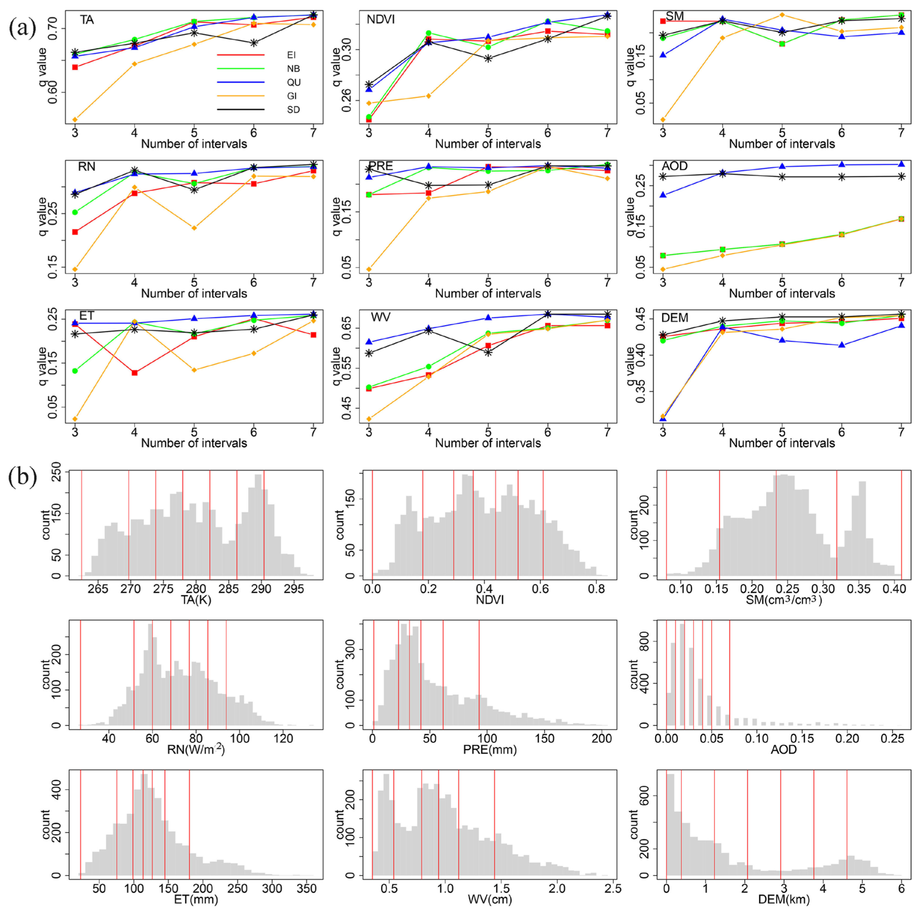
GeoDetector emphasizes the hierarchical and heterogeneous nature of spatial attributes. Therefore, when using GeoDetector analysis, it is necessary to discretize the input data for both the response and driving variables. However, it is difficult to obtain the optimal number of classifications in the discretization process. An excessive number of classifications would increase the computational burden and would be unnecessary, while a small number would fail to account for spatial diversity. Therefore, the choice of discretization method plays a key role [56]. To minimize uncertainty, we discretized the data with EI, QU, NB, GI, and SD, respectively, and finally chose the discretization method with the maximum q-value as the optimal solution. In this study, we discretize the continuous variables TA, NDVI, SM, RN, PRE, AOD, ET, WV, and DEM, while the type variables LULC and CLIMATE do not require any treatment. Take the 2003 data as an example to demonstrate the process of discretization of continuous variables. Figure 2 shows the process and results of discretizing the non-type variables for the potential drivers of LST.
The process of spatial discretization of each variable is shown in Figure 2a. By comparing various discretization methods, an optimum method for data discretization is selected with the number of cut points and discretization method corresponding to the maximum q-value. The results show that the optimal number of intervals for three variables, NDVI, PRE, and DEM, is 6, and the optimal interval for all the remaining variables is 7. The distribution of the optimal intervals for discretization of each variable is given in Figure 2b. Based on this, the potential driving factors at different spatial scales were all discretized in this study, and the discretized data at the optimal spatial scale were selected as the initial input data for the GeoDetector model to analyze the driving factors of spatial variability of LST. The optimal methods and breakpoint number for the discretization of each variable in 2003, 2008, 2013, and 2018 are summarized in Table 2, Table 3, Table 4 and Table 5.

4.2. Selection of Optimal Spatial Unit Scale

In geographic and spatial analysis, geographic variables at different spatial scales may show significantly different characteristics [57,58,59], a phenomenon known as “spatial scale effect”. As a spatial statistical method, GeoDetector is a method to analyze the spatial relationships between geographic phenomena and influencing factors, so it is necessary to select the best spatial scale for the analyzed data.
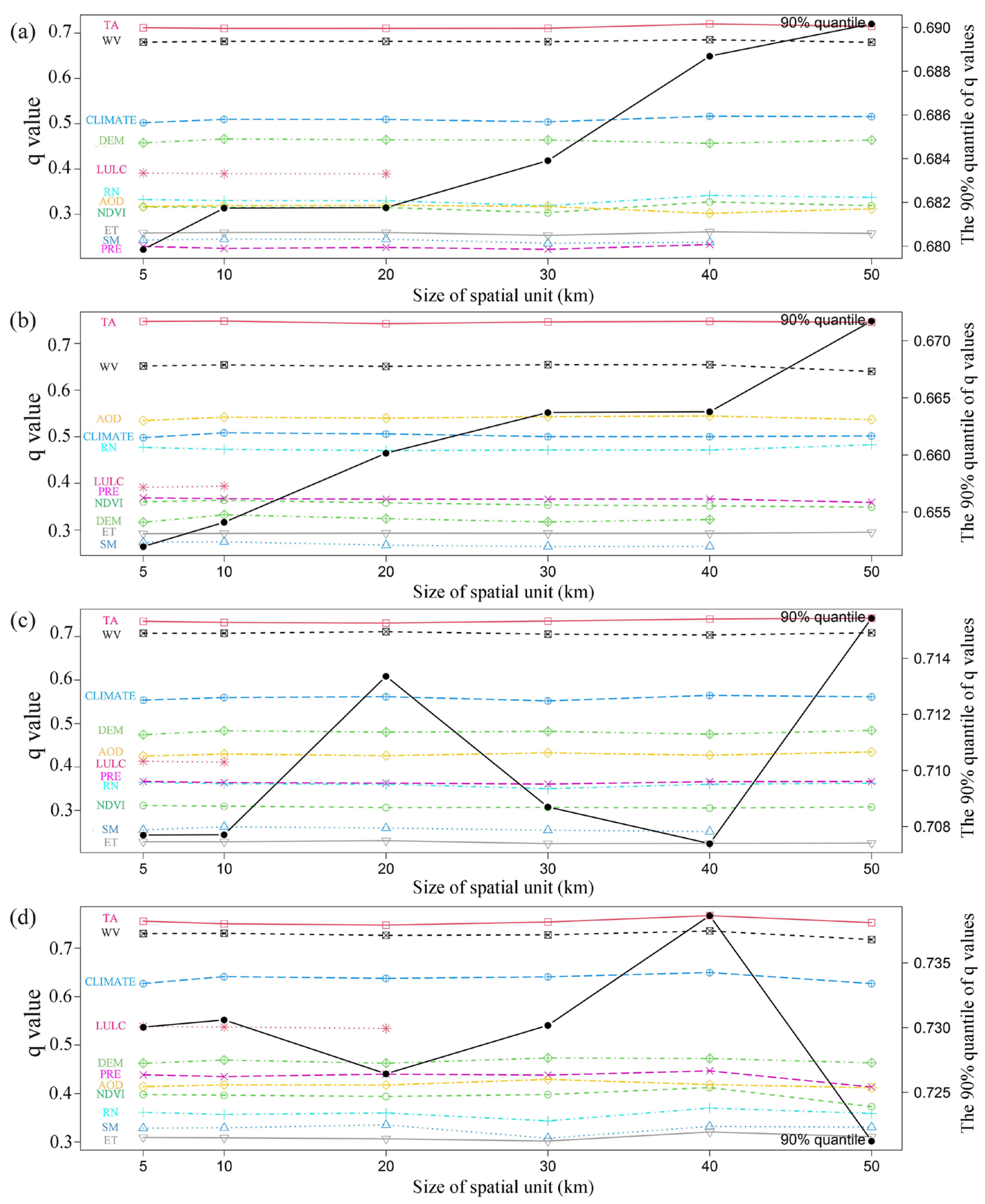
For GeoDetector, the optimal spatial scale selection is based on the assumption that the spatial scale corresponding to the highest q value of most drivers is the optimal spatial scale. In practice, the 90% quartile of the q-value of all drivers at different spatial scales is usually calculated and used to compare the trends of the q-value. The spatial scale corresponding to the highest value of the 90% quartile of the q-value for all drivers will be selected as the best spatial scale. In this study, six scales (5 km × 5 km, 10 km × 10 km, 20 km × 20 km, 30 km × 30 km, 40 km × 40 km, 50 km × 50 km) of grid data were selected as input variables for the GeoDetector model and used to obtain the optimal spatial scale for the study.
Figure 3 shows the variation in the q-value and their 90% quartile of the drivers at different spatial scales for each year. As shown in Figure 3a, the q-value of each driver corresponding to the spatial scale from 5 km to 10 km increased more significantly in 2003. The q-value of each variable did not change significantly from 10 km to 20 km, indicating that the influence of the variables on LST does not differ significantly at the spatial scale from 10 km to 20 km. However, LULC has no effect on the spatial distribution of LST at spatial scales up to 30 km. At spatial scales greater than 40 km, the driving effect of PRE on LST also disappears. When the spatial scale reaches 50 km, the 90% quartile of most of the driver q-values reaches its highest. Therefore, 50 km is then selected as the best spatial scale for the spatially differentiated driver analysis of LST in 2003. Similarly, the optimal spatial scales for 2008, 2013, and 2018 are 50 km, 50 km, and 40 km, respectively.

4.3. Impact of Individual Factor on the Spatial Heterogeneity of LST

In order to explore the drivers of LST spatial heterogeneity in China, environmental factors such as TA, NDVI, SM, RN, PRE, AOD, ET, WV, LULC, DEM, and CLIMATE were selected as potential drivers of LST in this study, and the relationship between each variable and LST was analyzed based on GeoDetector. The results of the FD give the contribution (q-value) of the drivers to the spatial heterogeneity of LST in 2003, 2008, 2013, and 2018. As shown in Figure 4, all q-values passed the significance test (p < 0.01).
The mean q-values of the effects for various factors on the spatial heterogeneity of LST were ranked as follows: TA (0.74) > WV (0.70) > CLIMATE (0.56) > DEM (0.44) > AOD (0.43) > RN (0.39) > NDVI (0.35) = PRE (0.35) > ET (0.28) = SM (0.28). In the selected years, TA has the largest q-value among all factors, indicating that TA is the most important factor influencing the spatial heterogeneity of LST. The effect of WV is the second largest for the years, which indicates that WV plays a moderating role in the LST spatial heterogeneity. The influence of CLIMATE is weaker than the two factors presented above, but it still has an indispensable role in LST spatial heterogeneity. Different climate types have different effects on LST spatial distribution. DEM does not show a dominant driving effect on LST, which may be due to the large spatial unit scale in this study, which weakens the strength of the effect of DEM. The q-value of AOD is second only to DEM, indicating that the effect of aerosols on LST is also a non-negligible part. The q-value of RN is smaller than we expect, which indicates that RN has a small effect on LST. In comparison, the effects of NDVI, PRE, ET, and SM on LST are also small in the selected years. The absence of LULC effects on LST spatial heterogeneity is due to the large spatial scale chosen for this study.
To understand the change of each driver’s contribution to LST, we calculated the rate of change of q-values of all drivers during the period 2003–2018, and the results showed that the overall trend in each driver’s contribution to LST from 2003 to 2018 was increasing, with PRE having the largest rate of change in q-value at 0.013/year, followed by CLIMATE with a rate of change of 0.009/year. NDVI, SM, and AOD have the same rate of change of 0.005/year. Comparing the q-values of all drivers individually within each year, it can be seen that the contribution of each driver fluctuated more in 2008 than in other years. Compared with 2003, the q-values of AOD, PRE, and RN increased by 0.13, 0.13, and 0.21, respectively, while the contribution of DEM decreased by 0.14. The statistics on the annual average values of the drivers showed that the annual average value of AOD in China reached 0.06 in 2008, which was significantly higher than that of 0.04 in 2003, while the absorbing aerosols increase the solar radiation received at the surface, which leads to an increase in the net radiation and thus a significant increase in the contribution to surface temperature. The decrease in the contribution of DEM is due to the increase in the optimal spatial scale to 50 km in 2008, at which the contribution of elevation to the spatial heterogeneity of LST is not significant. Except for the significant changes in most of the drivers in 2008, the contribution of drivers to LST in 2018 was higher than that in other years, and the most significant increase in the contribution of CLIMATE, PRE, and NDVI was observed. Table 6 provides detailed statistics on the contribution (q-value) of each driver to the spatial heterogeneity of LST and its rate of change from 2003 to 2018.

4.4. Effect of the Joint Factor on the Spatial Heterogeneity of LST

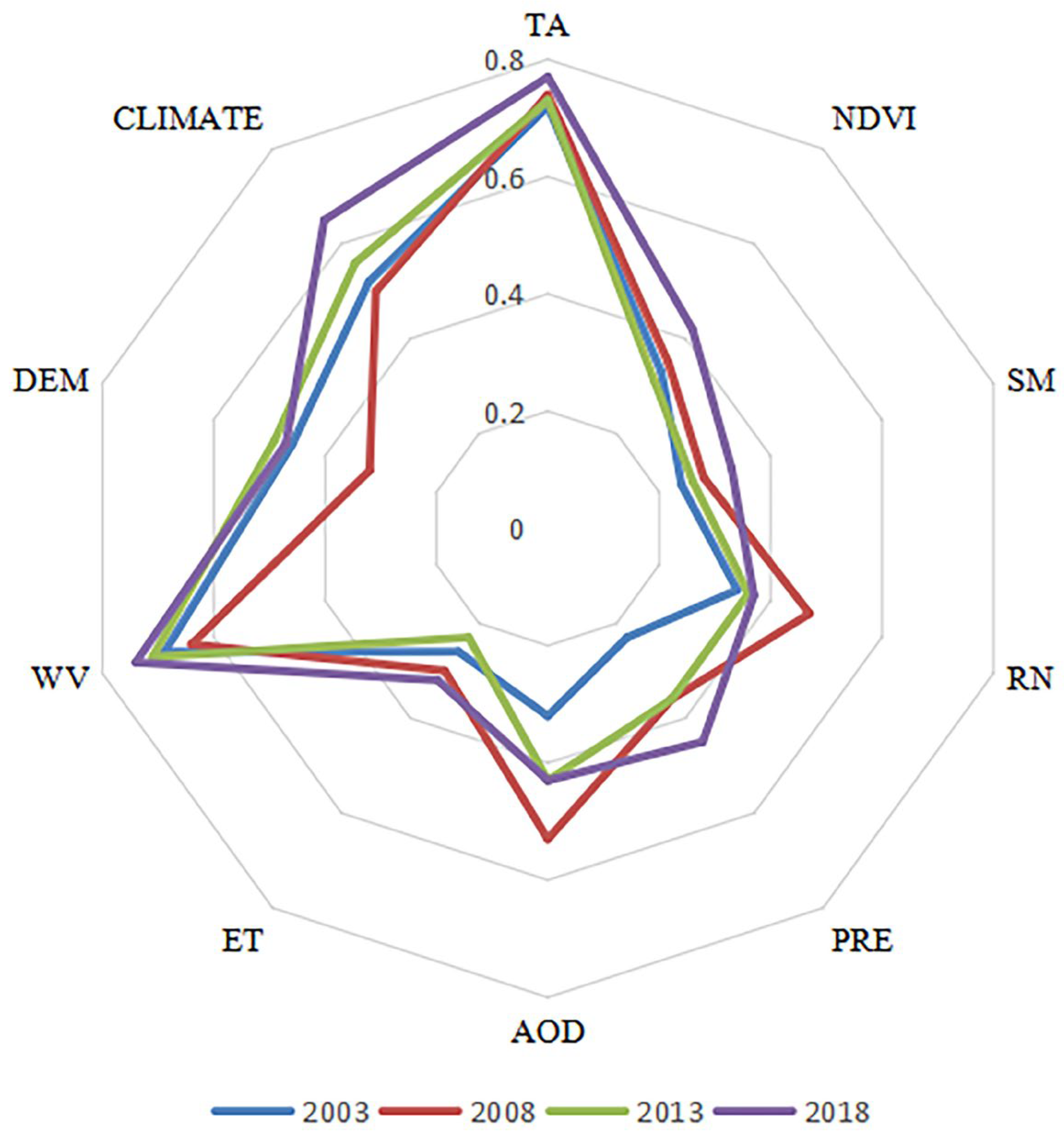
The ID was employed to reveal the interactive effect of drivers on LST and evaluate the explanatory ability of different factors on LST spatial heterogeneity. The q-values (q(X1∩X2)) of interaction in 2003, 2008, 2013, and 2018 are shown in Figure 5. The influence of the pairwise interaction of drivers on the LST spatial heterogeneity is stronger than that of any single factor, suggesting that the spatial heterogeneity of LST is jointly controlled by drivers rather than a single driver. Additionally, the type of the pairwise interaction during the period is dominated by bivariate enhancement.
Consistent with the individual contribution evaluation, TA had the most significant interaction effects with other factors in the selected years, and WV with other factors also had higher values. The interaction of drivers with TA all showed a large q-value (greater than 0.73) in each year, indicating TA still has a significant role in LST spatial changes. The largest q-value is the interaction between TA and LULC with values of 0.76, 0.80, 0.77, and 0.79 in 2003, 2008, 2013, and 2018. However, LULC does not show an effect on LST in individual contributions, indicating that LULC controls the spatial distribution of LST mainly through the combination with other factors at large scales and can dominate the role. The q-values of the interaction between WV and other factors also increased to a great extent, and the largest value is the interaction with TA. It is obvious from the results that there is a significant difference between individual contributions and joint contributions. In the individual factor effect, the q-values of NDVI, PRE, ET, and SM were relatively small. However, the joint effect of these factors had a noticeable increase in each year. It was shown that the effects of NDVI, PRE, ET, and SM on LST spatial heterogeneity were primarily attributed to the interaction with other factors.

4.5. Determine the Regions of the LST That Are Vulnerable to Drivers

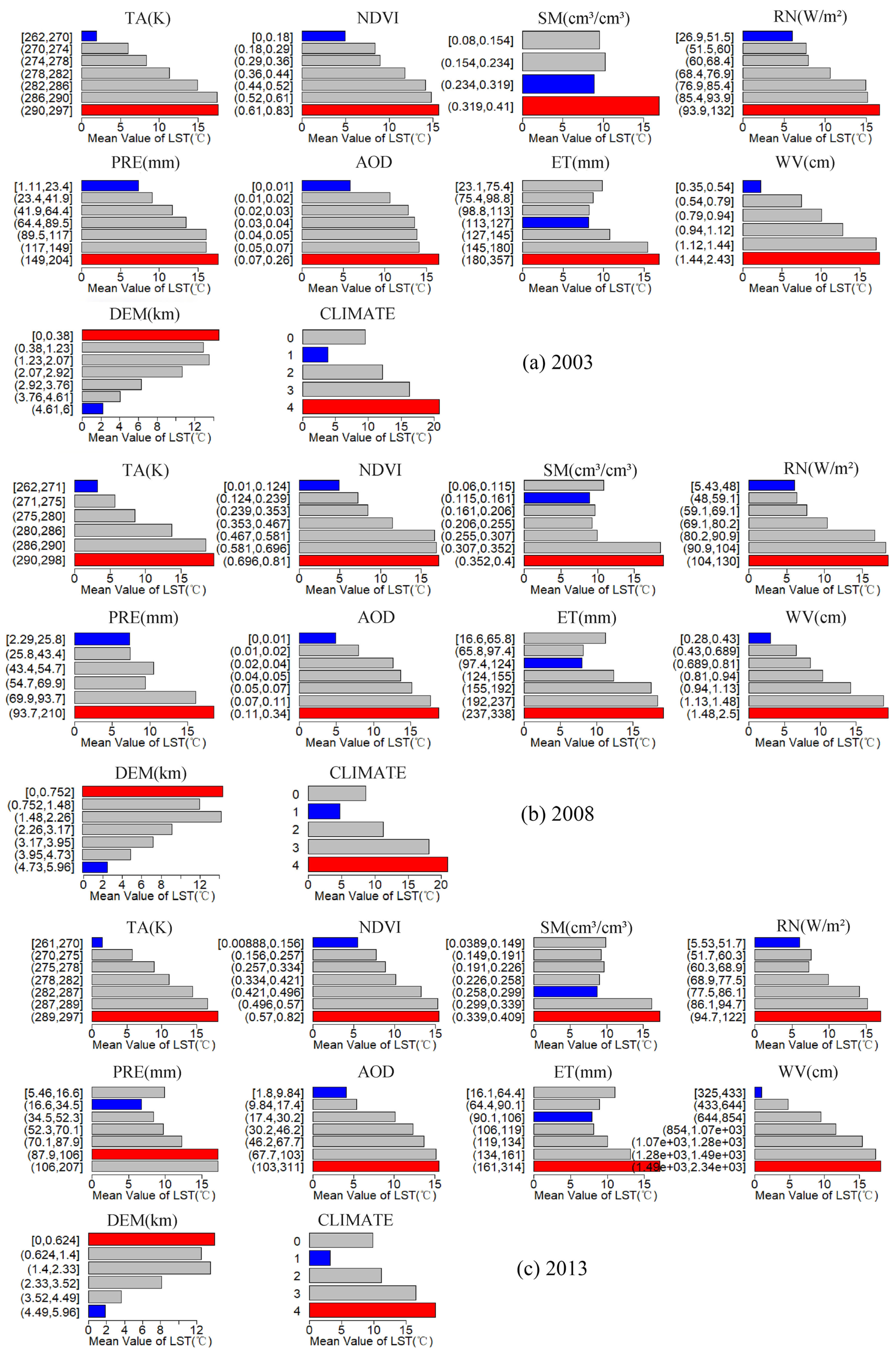
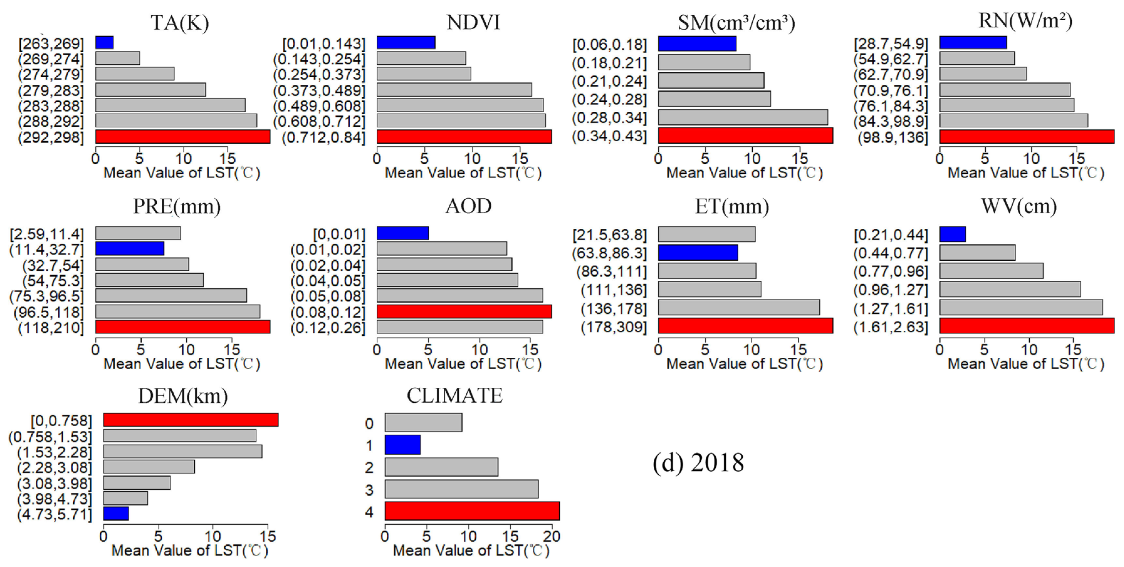
The RD provides the mean value of LST in the spatial region determined by the variables, and the results are shown in Figure 6. It shows that the same driver has a significantly different effect on LST in different intervals. Additionally, it can be seen that in each year, LST showed a positive correlation with TA, NDVI, RN, AOD, and WV in spatial distribution; i.e., the mean value of LST was also lower in regions with low values of driving variables, and conversely, the mean value of LST was also higher in regions with high values of driving variables. In contrast, LST and DEM showed a negative correlation in space, i.e., the higher the elevation, the lower the LST. The relationship between LST and SM and ET tends to decrease first and then increase, but the values of the turning points of the two relationships differed in each year, and overall LST showed a positive correlation with SM and ET when SM was greater than 0.25, and ET was greater than 120 mm. The effect of climate type on LST was lowest in the plateau mountainous climate zone and highest in the tropical monsoon climate zone.
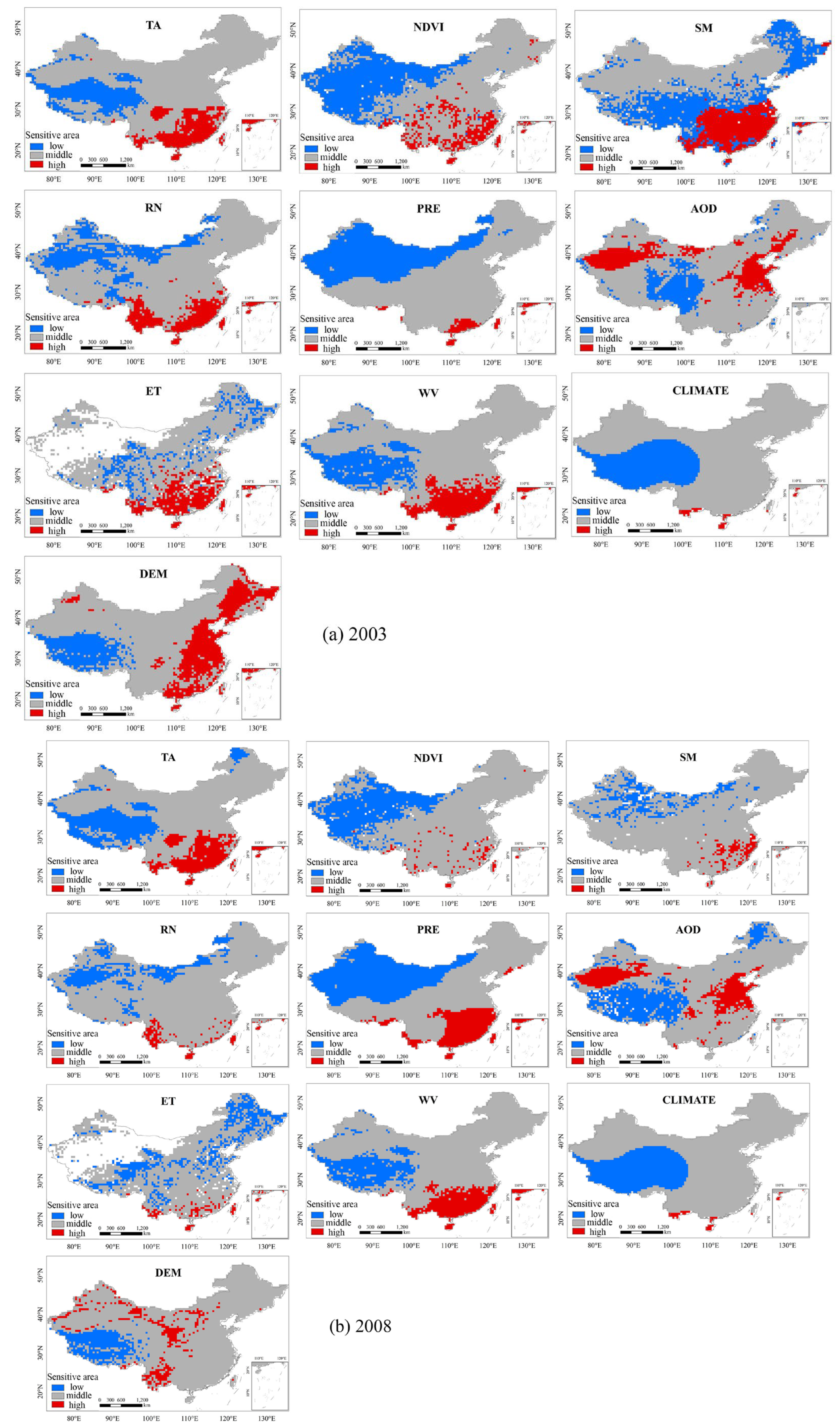
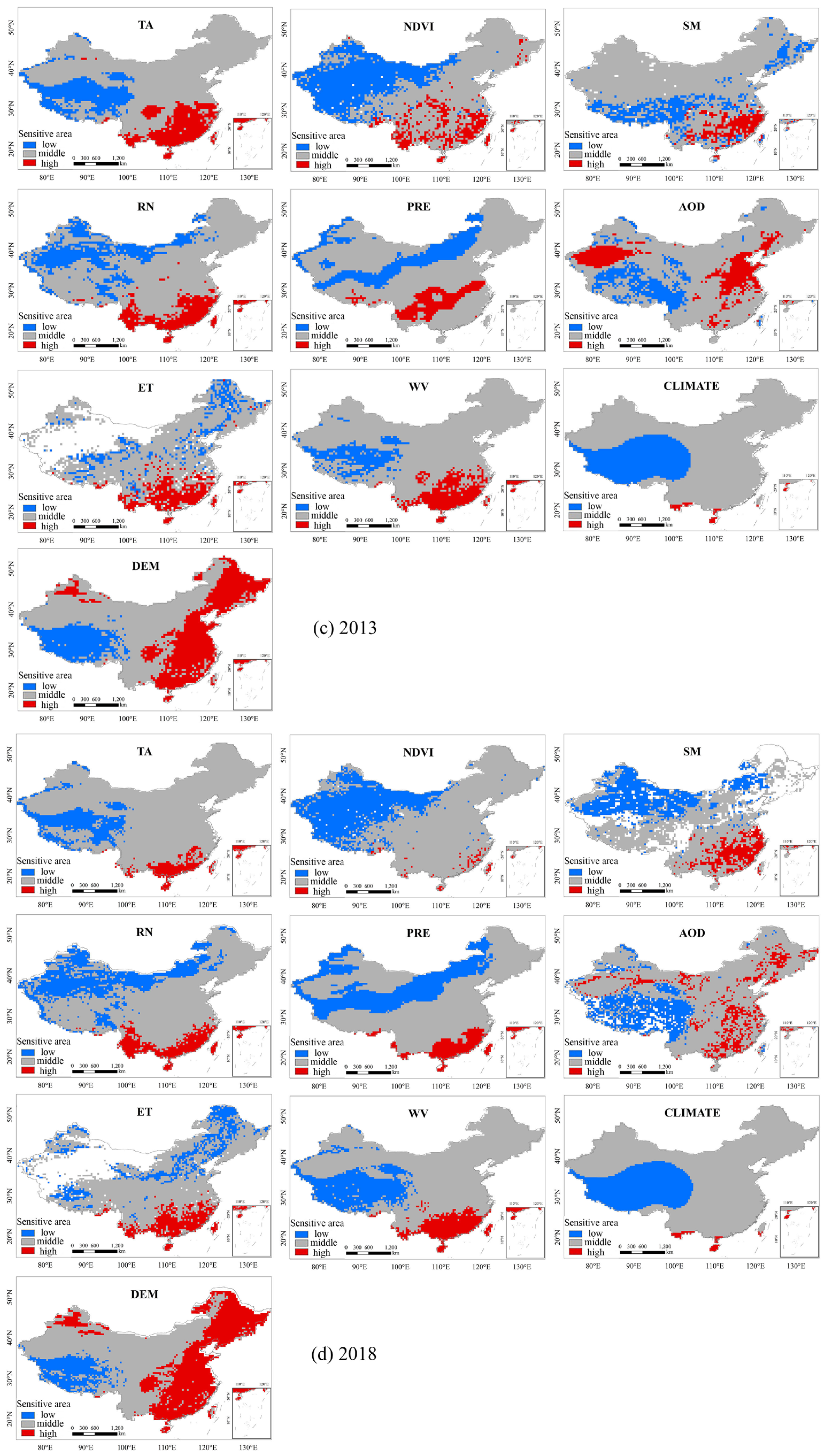
To further determine the geographical location of the LST-sensitive areas, we spatially displayed the average values of the LST determined by each driver in Figure 6, and obtained different sensitive areas of the LST response to each driver, as shown in Figure 7. The sensitive areas of LST are classified into three classes based on the influence of the drivers: high-sensitivity areas (red), medium-sensitivity areas (gray) and low-sensitivity areas (blue). From the spatial distribution of sensitive areas of LST in each year, the distribution patterns of risk partitioning of LST determined by most of the drivers are similar; that is, the drivers have relatively weak driving effects on LST in the northwest of China and stronger driving effects in the tropical and subtropical regions in the south. However, the two drivers of AOD and DEM are different. In the period 2003 to 2013, the high-sensitivity areas of AOD on LST are mainly distributed in the northwest desert and Beijing–Tianjin–Hebei region. However, by 2018, the impact of AOD on LST is significantly weakened, and the highly sensitive areas in the northwest and Beijing–Tianjin–Hebei region are significantly reduced, mostly showing a non-concentrated distribution pattern, which may be closely related to the environmental management in the above regions, and the reduction in haze, sand and dust weather has reduced the overall AOD and weakened the impact on LST. Regions with higher impact of DEM on LST are mainly distributed in the eastern plains, and the regions with lower impact are mainly distributed in the eastern plains. The high-sensitivity area of CLIMATE on LST is only in the tropical monsoon climate area.

5. Discussions

This study aimed to identify the influencing factors of LST spatial heterogeneity in China from the period 2003–2018 and, further, to explore the manner and strength of the influencing factors on LST.
According to GeoDetector analysis, TA shows the strongest effect on LST spatial heterogeneity. Unlike other studies that considered DEM as the main influencing factor [60,61], which indicates that the energy exchange between land and atmosphere is stronger than other factors. The effect of TA on LST is stronger in the south of China than that in the northwest areas. WV also has a big effect on LST spatial heterogeneity, but it has often been overlooked before now. CLIMATE is a common factor that drives both the spatial and temporal distribution of LST [62,63]. The gradient characteristics of temperature with surface elevation are often used by researchers as a basis for LST spatial interpolation [64,65]. In this study, although DEM did not reflect a dominant contribution to the spatial distribution of LST, it also showed a significant negative correlation with LST, i.e., low LST in regions with high DEM. In particular, the interaction with other factors greatly enhanced the control of the spatial distribution of LST.
In general, RN and NDVI should have a relatively large effect on LST [66,67]. However, the result shows that the RN and NDVI as a single factor on LST were relatively small during the study period. RN is gradually changing with latitude in spatial distribution, resulting in a weak effect of RN on LST. Additionally, the larger pixel scale attenuates its vegetation characteristics, weakening the influence of NDVI on the spatial heterogeneity of LST. PRE is also a key driving factor of LST, but it is generally concentrated during the monsoon season, thus leading a weak impact on LST from the yearly scale. As for SM and ET, they were also limited by the seasonal change. In addition, the completeness of the data for both is poor, which also affects the results of the study. The effect of AOD on the temporal variation in LST was not remarkable, but the effect on the spatial distribution of LST either as a single factor or interacting with other factors could not be ignored. This may be attributed to its obvious spatial distribution characteristics, which are concentrated in the northwest and Beijing–Tianjin–Hebei region, thus enhancing the controlling of the spatial distribution of LST. In addition, in the current study, data from 2003, 2008, 2013, and 2018 were selected to analyze the driving effect of each factor on LST, indirectly analyzing the role of interannual variation in each factor on the spatial heterogeneity of LST, and therefore, the effect of interannual variation in each variable was not considered separately.
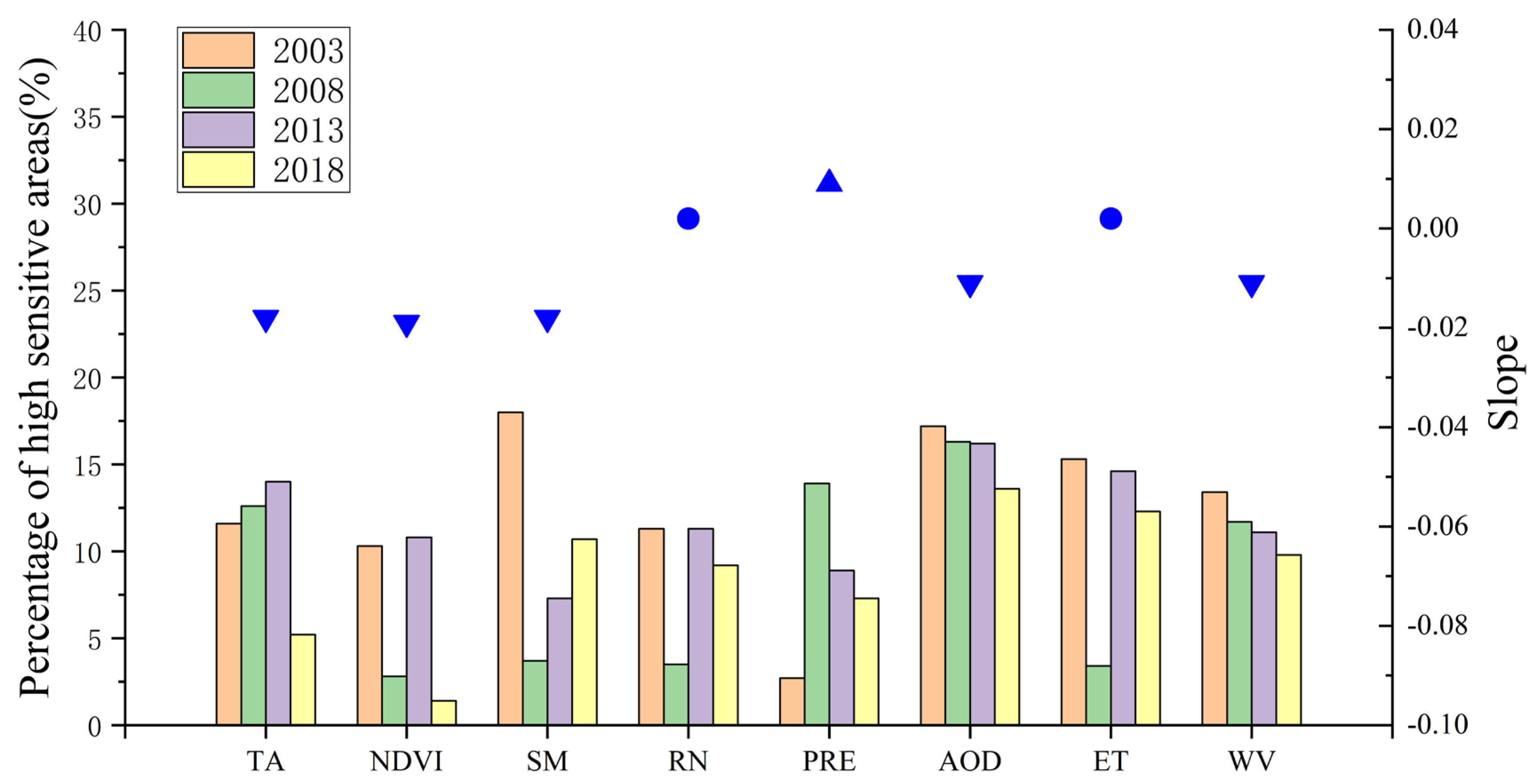
To further determine the variation in the highly sensitive regions of LST in response to key drivers over time, we counted the percentage of highly sensitive areas of LST in response to each driver for the selected years, and the results are shown in Figure 8. Due to DEM and CLIMATE being relatively stable drivers, they are hardly affected by time. Therefore, only the sensitive areas of the LST in response to TA, NDVI, SM, RN, PRE, AOD, ET, and WV are analyzed over time. Among them, the proportion of highly sensitive areas of LST to TA, NDVI, SM, AOD, and WV showed a decreasing trend from 2003 to 2018, while the areas of PRE showed an increasing trend. The trend in the proportion of highly sensitive areas to RN and ET did not change significantly overall. In terms of the areas of LST with high sensitivity to each driver, LST was driven by AOD the most, with an average share of 15.8%, followed by WV, with an average share of 11.5%. The share of high-sensitivity areas driven by TA and ET was similar, about 11%, and the share of high-sensitivity areas driven by the remaining factors was less than 10%. The trend in the highly sensitive areas showed that AOD and WV decreased year by year with a slope of −0.01/year, while TA, NDVI, and SM also showed a decreasing trend, but with greater fluctuations from year to year.
Overall, an important finding on the spatial heterogeneity of LST in China is provided in this study. However, there are still some limitations in this study. LST is a complicated variable and is influenced by different factors. However, while this study explores the driving effect of influence factors on the spatial heterogeneity of LST at the annual scale, some factors have different effects on LST in different seasons, and the differences in the driving effect of factors at the seasonal level remain unclear. Moreover, LULC is a key influence factor for the spatial heterogeneity of LST, but the large spatial unit scale in this study limits the driving effect of LULC, so it is necessary to explore and compare the effect of the drivers on LST at different spatial scales. In addition, the lack of LST and influence factors data also partly affected the accuracy of the results, and although the product quality file was used and integrated data to an annual scale in the study, there are some pixels that are affected by clouds causing uneven spatial distribution. Therefore, to ensure the accuracy of the results, it is crucial to use full spatial coverage data or develop high-precision data reconstruction methods.

6. Conclusions

In this study, GeoDetector was used to analyze the drivers of LST spatial heterogeneity in China for 2003, 2008, 2013, and 2018. The main findings are as follows:
(1)
The factor detector showed that the explanatory ability of the drivers (TA, WV, CLIMATE, DEM, AOD, RN, NDVI, PRE, ET, and SM) indicates that TA has the greatest driving effect in the selected years, and the driving strength is increasing at a rate of 0.003/year. WV is second only to TA and also shows a strong driving effect on LST spatial heterogeneity with a change rate of 0.004/year. LULC has no driving effect on LST spatial heterogeneity due to the spatial unit scale.
(2)
The interaction detector revealed that the effect of the interaction is significantly greater than the effect of any single factor, which indicates that the spatial heterogeneity of LST is the result of multi-factor interactions. Similarly to the individual effect, TA has the strongest joint effect with other factors, especially the interaction with LULC, with a mean q-value of 0.78.
(3)
The risk detector found that the sensitive areas of LST determined by the driving factor have a similar spatial distribution pattern. However, variations in the high-sensitivity regions exist from year to year. During the study period, LST was driven by AOD over the widest area, with an average share of 15.8%, followed by WV, with an average share of 11.5%. Overall, the high-sensitivity areas determined by most drivers showed a decreasing trend.
Generally, this study provides a unique insight into the spatial heterogeneity of LST in China. The results of the study on LST spatial heterogeneity drivers can provide new directions for the selection of methods for climate warming mitigation, land use practices, and drought prediction.

Author Contributions

Writing—original draft preparation, Y.Y.; writing—review and editing, Y.Y., S.F. and W.Z.; visualization, Y.Y.; formal analysis, Y.Y.; data curation, W.Z.; supervision, S.F. All authors have read and agreed to the published version of the manuscript.

Funding

This research received no external funding.

Data Availability Statement

Not applicable.

Acknowledgments

The authors would like to thank the reviewers and the handling editor, whose comments and suggestions improved this paper.

Conflicts of Interest

The authors declare no conflict of interest.

References

  1. Townshend, J.R.G.; Justice, C.O.; Skole, D.; Malingreau, J.P.; Cihlar, J.; Teillet, P.; Sadowski, F.; Ruttenberg, S. The 1 km resolution global data set: Needs of the International Geosphere Biosphere Programme. Int. J. Remote Sens. 1994, 15, 3417–3441. [Google Scholar] [CrossRef]
  2. Anderson, M.; Norman, J.; Kustas, W.; Houborg, R.; Starks, P.; Agam, N. A thermal-based remote sensing technique for routine mapping of land-surface carbon, water and energy fluxes from field to regional scales. Remote Sens. Environ. 2008, 112, 4227–4241. [Google Scholar] [CrossRef]
  3. Zhang, Q.; Xu, C.Y.; Zhang, Z.; Chen, Y.D. Changes of temperature extremes for 1960–2004 in Far-West China. Stoch. Environ. Res. Risk Assess. 2008, 23, 721–735. [Google Scholar] [CrossRef]
  4. Li, Z.-L.; Tang, B.-H.; Wu, H.; Ren, H.; Yan, G.; Wan, Z.; Trigo, I.F.; Sobrino, J.A. Satellite-derived land surface temperature: Current status and perspectives. Remote Sens. Environ. 2013, 131, 14–37. [Google Scholar] [CrossRef]
  5. Karnieli, A.; Agam, N.; Pinker, R.; Anderson, M.; Imhoff, M.; Gutman, G.; Panov, N.; Goldberg, A. Use of NDVI and land surface temperature for drought assessment: Merits and limitations. J. Clim. 2010, 23, 618–633. [Google Scholar] [CrossRef]
  6. Peng, W.; Zhou, J.; Wen, L.; Xue, S.; Dong, L. Land surface temperature and its impact factors in Western Sichuan Plateau, China. Geocarto Int. 2016, 32, 919–934. [Google Scholar] [CrossRef]
  7. Zhao, H.; Ren, Z.; Tan, J. The spatial patterns of land surface temperature and its impact factors: Spatial non-stationarity and scale effects based on a Geographically-Weighted Regression model. Sustainability 2018, 10, 2242. [Google Scholar] [CrossRef]
  8. Guha, S.; Govil, H.; Diwan, P. Monitoring LST-NDVI relationship using premonsoon Landsat datasets. Adv. Meteorol. 2020, 2020, 4539684. [Google Scholar] [CrossRef]
  9. Yang, Y.; Park, J.; An, S.; Wang, B.; Luo, X. Mean sea surface temperature changes influence ENSO-related precipitation changes in the mid-latitudes. Nat. Commun. 2021, 12, 1495. [Google Scholar] [CrossRef]
  10. Juang, J.Y.; Katul, G.; Siqueira, M.; Stoy, P.; Novick, K. Separating the effects of albedo from eco-physiological changes on surface temperature along a successional chrono sequence in the southeastern United States. Geophys. Res. Lett. 2007, 34, 1–5. [Google Scholar] [CrossRef]
  11. Peng, S.S.; Piao, S.; Zeng, Z.; Ciais, P.; Zhou, L.; Li, L.Z.; Myneni, R.B.; Yin, Y.; Zeng, H. Afforestation in China cools local land surface temperature. Proc. Natl. Acad. Sci. USA 2014, 111, 2915–2919. [Google Scholar] [CrossRef] [PubMed]
  12. Liu, Y.; Zhang, Y.; Zhu, J.; Huang, K.; Zu, J.; Chen, N.; Cong, N.; Stegehuis, A. Warming slowdown over the Tibetan plateau in recent decades. Theor. Appl. Climatol. 2018, 135, 1375–1385. [Google Scholar] [CrossRef]
  13. Feng, Y.; Gao, C.; Tong, X.; Chen, S.; Lei, Z.; Wang, J. Spatial patterns of land surface temperature and their influencing factors: A case study in Suzhou, China. Remote Sens. 2019, 11, 182. [Google Scholar] [CrossRef]
  14. Zhou, W.Q.; Husng, G.L.; Cadenasso, M.L. Does spatial configuration matter? Understanding the effects of land cover pattern on land surface temperature in urban landscapes. Landsc. Urban Plan 2011, 102, 54–63. [Google Scholar] [CrossRef]
  15. Yan, Y.; Mao, K.; Shi, J.; Piao, S.; Shen, X.; Dozier, J.; Liu, Y.; Ren, L.-H.; Bao, Q. Driving forces of land surface temperature anomalous changes in North America in 2002–2018. Sci. Rep. 2020, 10, 6391. [Google Scholar] [CrossRef]
  16. Zhi, Y.; Shan, L.; Ke, L.; Yang, R. Analysis of Land Surface Temperature Driving Factors and Spatial Heterogeneity Research Based on Geographically Weighted Regression Model. Complexity 2020, 2020, 2862917. [Google Scholar] [CrossRef]
  17. Yu, Y.; Shang, G.; Duan, S.; Yu, W.; Labed, J.; Li, Z. Quantifying the Influences of Driving Factors on Land Surface Temperature during 2003–2018 in China Using Convergent Cross Mapping Method. Remote Sens. 2022, 14, 3280. [Google Scholar] [CrossRef]
  18. Brunsdon, C.; Fotheringham, A.S.; Charlton, M.E. Geographically weighted regression: A method for exploring spatial nonstationarity. Geogr. Anal. 1996, 28, 281–298. [Google Scholar] [CrossRef]
  19. Goovaerts, P.; Xiao, H.; Adunlin, G.; Ali, A.; Tan, F.; Gwede, C.K.; Huang, Y. Geographically-weighted regression analysis of percentage of late-stage prostate cancer diagnosis in florida. Appl. Geogr. 2015, 62, 191–200. [Google Scholar] [CrossRef]
  20. Zhao, Z.; Gao, J.; Wang, Y.; Liu, J.; Li, S. Exploring spatially variable relationships between NDVI and climatic factors in a transition zone using geographically weighted regression. Theor. Appl. Climatol. 2015, 120, 507–519. [Google Scholar] [CrossRef]
  21. Javi, S.T.; Malekmohammadi, B.; Mokhtari, H. Application of geographically weighted regression model to analysis of spatiotemporal varying relationships between groundwater quantity and land use changes (case study: Khanmirza Plain, Iran). Environ. Monit. Assess. 2014, 186, 3123–3138. [Google Scholar] [CrossRef] [PubMed]
  22. Zhou, X.; Wang, Y. Dynamics of land surface temperature in response to land-use/cover change. Geogr. Res. 2010, 49, 23–36. [Google Scholar] [CrossRef]
  23. Li, S.; Zhao, Z.; Miao, X.; Wang, Y. Investigating spatial non-stationary and scale-dependent relationships between urban surface temperature and environmental factors using geographically weighted regression. Environ. Model. Softw. 2010, 25, 1789–1800. [Google Scholar] [CrossRef]
  24. Szymanowski, M.; Kryza, M. Application of geographically weighted regression for modelling the spatial structure of urban heat island in the city of Wroclaw (SW Poland). Procedia Environ. Sci. 2011, 3, 87–92. [Google Scholar] [CrossRef]
  25. Ivajnšič, D.; Kaligarič, M.; Žiberna, I. Geographically weighted regression of the urban heat island of a small city. Appl. Geogr. 2014, 53, 41–353. [Google Scholar] [CrossRef]
  26. Wang, J.F.; Zhang, T.L.; Fu, B.J. A measure of spatial stratified heterogeneity. Ecol. Indic. 2016, 67, 250–256. [Google Scholar] [CrossRef]
  27. Yang, D.; Wang, X.; Xu, J.; Xu, C.; Lu, D.; Ye, C.; Wang, Z.; Bai, L. Quantifying the influence of natural and socioeconomic factors and their interactive impact on PM2.5 pollution in China. Environ. Pollut. 2018, 241, 475–483. [Google Scholar] [CrossRef]
  28. Luo, W.; Jasiewicz, J.; Stepinski, T.; Wang, J.; Xu, C.; Cang, X. Spatial association between dissection density and environmental factors over the entire conterminous United States. Geophys. Res. Lett. 2016, 43, 692–700. [Google Scholar] [CrossRef]
  29. Wang, W.; Samat, A.; Abuduwaili, J.; Ge, Y. Spatio-temporal variations of satellite-based PM2.5 concentrations and its determinants in Xinjiang, northwest of China. Int. J. Environ. Res. Public Health 2020, 17, 2157. [Google Scholar] [CrossRef]
  30. Yang, J.; Ren, J.; Sun, D.; Xiao, X.; Xia, J.; Jin, C.; Li, X. Understanding land surface temperature impact factors based on local climate zones. Sustain. Cities Soc. 2021, 69, 102818. [Google Scholar] [CrossRef]
  31. Wu, Z.; Man, W.; Ren, Y. Detection of spatial-temporal variations in forest canopy surface temperature in response to urbanization: A case study from Longyan, China. J. Environ. Plan. Manag. 2019, 63, 1283–1300. [Google Scholar] [CrossRef]
  32. Chen, L.; Wang, X.; Cai, X.; Yang, C.; Lu, X. Seasonal variations of daytime land surface temperature and their underlying drivers over Wuhan, China. Remote Sens. 2021, 13, 323. [Google Scholar] [CrossRef]
  33. Wang, J.; Zhao, J.; Zhou, P.; Li, K.; Cao, Z.; Zhang, H.; Han, Y.; Luo, Y.; Yuan, X. Study on the Spatial and Temporal Evolution of NDVI and Its Driving Mechanism Based on Geodetector and Hurst Indexes: A Case Study of the Tibet Autonomous Region. Sustainability 2023, 15, 5981. [Google Scholar] [CrossRef]
  34. Wan, Z.; Li, Z.-L. A physics-based algorithm for retrieving land-surface emissivity and temperature from EOS/MODIS data. IEEE Trans. Geosci. Remote Sens. 1997, 35, 980–996. [Google Scholar] [CrossRef]
  35. Wan, Z.; Zhang, Y.; Zhang, Q.; Li, Z.L. Validation of the land-surface temperature products retrieved from Terra Moderate Resolution Imaging Spectroradiometer data. Remote Sens. Environ. 2002, 83, 163–180. [Google Scholar] [CrossRef]
  36. Wan, Z.; Li, Z.-L. Radiance-based validation of the V5 MODIS land surface temperature product. Int. J. Remote Sens. 2008, 29, 5373–5395. [Google Scholar] [CrossRef]
  37. Wan, Z.; Li, Z.-L. MODIS land surface temperature and emissivity. In Land Remote Sensing and Global Environmental Change; Springer: Berlin/Heidelberg, Germany, 2010; pp. 563–577. [Google Scholar]
  38. Carlson, T.N.; Ripley, D.A. On the relation between NDVI, fractional vegetation cover, and leaf area index. Remote Sens. Environ. 1997, 62, 241–252. [Google Scholar] [CrossRef]
  39. Chen, Y.; Xia, J.; Liang, S.; Feng, J.; Fisher, J.B.; Li, X.; Li, X.; Liu, S.; Ma, Z.; Miyata, A. Comparison of satellite-based evapotranspiration models over terrestrial ecosystems in China. Remote Sens. Environ. 2014, 140, 279–293. [Google Scholar] [CrossRef]
  40. Dorigo, W.; Wagner, W.; Albergel, C.; Albrecht, F.; Balsamo, G.; Brocca, L.; Chung, D.; Ertl, M.; Forkel, M.; Gruber, A. ESA CCI Soil Moisture for improved Earth system understanding: State-of-the art and future directions. Remote Sens. Environ. 2017, 203, 185–215. [Google Scholar] [CrossRef]
  41. Liu, Y.Y.; Dorigo, W.A.; Parinussa, R.M.; DeJeu, R.A.M.; Wagner, W.; McCabe, M.F.; Evans, J.P.; Van Dijk, A.I.J.M. Trend-preserving blending of passive and active microwave soil moisture retrievals. Remote Sens. Environ. 2012, 123, 280–297. [Google Scholar] [CrossRef]
  42. An, R.; Zhang, L.; Wang, Z.; Quaye-Ballard, J.A.; You, J.; Shen, X.; Gao, W.; Huang, L.; Zhao, Y.; Ke, Z. Validation of the ESA CCI soil moisture product in China. Int. J. Appl. Earth Obs. Geoinf. 2016, 48, 28–36. [Google Scholar] [CrossRef]
  43. Albergel, C.; Dorigo, W.; Reichle, R.H.; Balsamo, G.; De Rosnay, P.; Munoz-Sabater, J.; Isaksen, L.; De Jeu, R.; Wagner, W. Skill and Global Trend Analysis of Soil Moisture from Reanalyses and Microwave Remote Sensing. J. Hydrometeorol. 2013, 14, 1259–1277. [Google Scholar] [CrossRef]
  44. Harris, I.; Osborn, T.J.; Jones, P.; Lister, D. Version 4 of the CRU TS monthly high-resolution gridded multivariate climate dataset. Sci. Data 2020, 7, 109. [Google Scholar] [CrossRef]
  45. Li, X.; Zhou, Y.; Asrar, G.R.; Zhu, Z. Developing a 1 km resolution daily air temperature dataset for urban and surrounding areas in the conterminous United States. Remote Sens. Environ. 2018, 215, 74–84. [Google Scholar] [CrossRef]
  46. Parker, J.; Kenyon, R.V.; Troxel, D.E. Comparison of interpolating methods for image resampling. IEEE Trans. Med. Imaging 1983, 2, 31–39. [Google Scholar] [CrossRef] [PubMed]
  47. Wang, J.; Li, X.H.; Christakos, G.; Liao, Y.; Zhang, T.; Gu, X.; Zheng, X. Geographical Detectors-Based Health Risk Assessment and its Application in the Neural Tube Defects Study of the Heshun Region, China. Int. J. Geogr. Inf. Sci. 2010, 24, 107–127. [Google Scholar] [CrossRef]
  48. Wang, J.; Hu, Y. Environmental health risk detection with GeoDetector. Environ. Model. Softw. 2012, 33, 114–115. [Google Scholar] [CrossRef]
  49. Liao, Y.L.; Wang, J.F.; Guo, Y.Q.; Zheng, X.Y. Risk Assessment of Human Neural Tube Defects Using a Bayesian Belief Network. Environ. Res. Risk Assess. 2010, 24, 93–100. [Google Scholar] [CrossRef]
  50. Kerber, R. Chimerge: Discretization of numeric attributes. In Proceedings of the Tenth National Conference on Artificial Intelligence, San Jose, CA, USA, 12–16 July 1992; AAAI Press: Menlo Park, CA, USA, 1992; pp. 123–128. [Google Scholar]
  51. Dougherty, J.; Kohavi, R.; Sahami, M. Supervised and unsupervised discretization of continuous features. In Proceedings of the Twelfth International Conference on Machine Learning, Tahoe City, CA, USA, 9–12 July 1995; Morgan Kaufmann Publisher: San Francisco, CA USA, 1995; pp. 194–202. [Google Scholar] [CrossRef]
  52. Kurgan, L.A.; Cios, K.J. Discretization algorithm that uses class-attribute interdependence maximization. IEEE Trans. Knowl. Data Eng. 2004, 16, 145153. [Google Scholar] [CrossRef]
  53. Tsai, C.J.; Lee, C.I.; Yang, W.P. A discretization algorithm based on Class-Attribute Contingency Coefficient. Inf. Sci. 2008, 178, 714–731. [Google Scholar] [CrossRef]
  54. Ge, Y.; Cao, F.; Duan, R.F. Impact of discretization methods on the rough set-based classification of remotely sensed images. Int. J. Digit. Earth 2011, 4, 330–346. [Google Scholar] [CrossRef]
  55. Fisher, M.M.; Wang, J.F. Spatial Data Analysis: Models, Methods and Techniques; Springer: Berlin, Germany, 2011; p. 82. [Google Scholar]
  56. Jenks, G.F. The data model concept in statistical mapping. Int. Yearb. Cartogr. 1967, 7, 186–190. [Google Scholar]
  57. Cao, F.; Ge, Y.; Wang, J. Optimal discretization for geographical detectors-based risk assessment. GISci. Remote Sens. 2013, 50, 78–92. [Google Scholar] [CrossRef]
  58. Roth, N.E.; David, A.J.; Erickson, D.L. Landscape influences on stream biotic integrity assessed at multiple spatial scales. Landsc. Ecol. 1996, 11, 141–156. [Google Scholar] [CrossRef]
  59. Store, R.; Jokimäki, J. A GIS-based multi-scale approach to habitat suitability modeling. Ecol. Model. 2003, 169, 1–15. [Google Scholar] [CrossRef]
  60. Chen, Q.; Mcroberts, R.; Wang, C.; Radtke, P. Forest aboveground biomass mapping and estimation across multiple spatial scales using model-based inference. Remote Sens. Environ. 2016, 184, 350–360. [Google Scholar] [CrossRef]
  61. Xu, Y.; Shen, Y.; Wu, Z. Spatial and temporal variations of land surface temperature over the Tibetan plateau based on harmonic analysis. Mt. Res. Dev. 2013, 33, 85–94. [Google Scholar] [CrossRef]
  62. Yang, M.; Zhao, W.; Zhan, Q.; Xiong, D. Spatiotemporal patterns of land surface temperature change in the Tibetan plateau based on MODIS/Terra daily product from 2000 to 2018. IEEE J. Sel. Top. Appl. Earth Obs. Remote Sens. 2021, 14, 6501–6514. [Google Scholar] [CrossRef]
  63. Xing, Z.; Yu, Y.; Duan, S.-B.; Li, Z.-L.; Gao, M.; Leng, P.; Shang, G. Modeling year-to-year variations of clear-sky land surface temperature using Aqua/MODIS data. IEEE Access 2020, 8, 114541–114553. [Google Scholar] [CrossRef]
  64. Yu, Y.; Duan, S.; Li, Z.; Chang, S.; Xing, Z.; Leng, P.; Gao, M. Interannual spatiotemporal variations of land surface temperature in China from 2003 to 2018. IEEE J. Sel. Top. Appl. Earth Obs. Remote Sens. 2021, 14, 1783–1795. [Google Scholar] [CrossRef]
  65. Xu, Y.; Knudby, A.; Shen, Y.; Liu, Y. Mapping monthly air temperature in the Tibetan Plateau from MODIS data based on machine learning methods. IEEE J. Sel. Top. Appl. Earth Obs. Remote Sens. 2018, 11, 345–354. [Google Scholar] [CrossRef]
  66. Gttsche, F.M.; Olesen, F.S. Modelling the effect of optical thickness on diurnal cycles of land surface temperature. Remote Sens. Environ. 2009, 113, 2306–2316. [Google Scholar] [CrossRef]
  67. Zhang, W.; Yi, S.-H.; Qin, Y.; Shangguan, D.-H.; Qin, Y. Analysis of features and influencing factors of alpine meadow surface temperature based on UAV thermal thermography. Acta Prataculturae Sin. 2021, 30, 15–27. [Google Scholar]
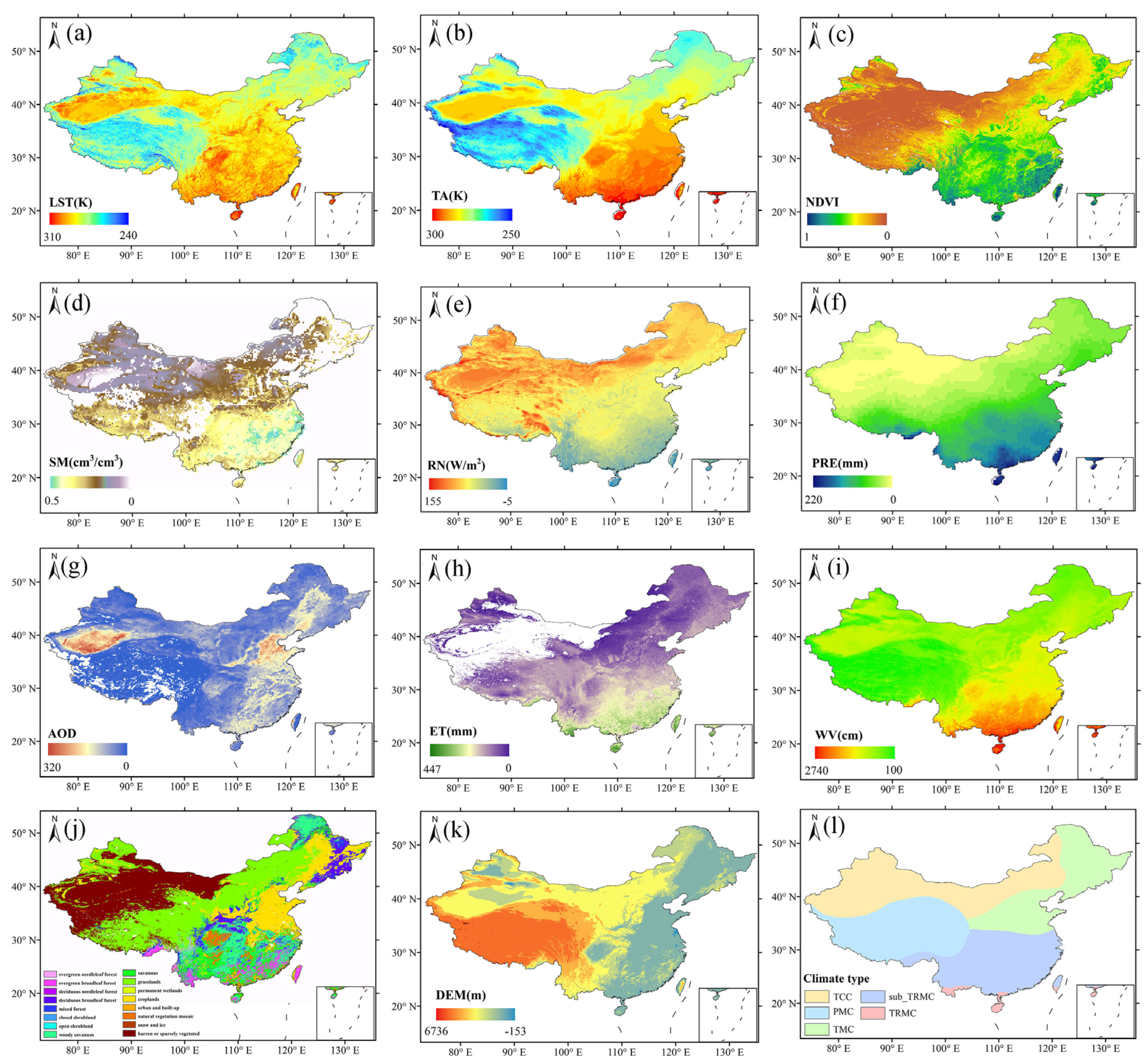
Figure 1. Spatial distribution of (a) annual mean LST, (b) annual mean air temperature, (c) annual mean NDVI, (d) annual mean soil moisture, (e) annual mean net surface radiation, (f) annual mean precipitation, (g) annual mean AOD, (h) annual mean evaporation, (i) annual mean water vapor, (j) land cover, (k) elevation, and (l) climate types.
Remotesensing 15 02814 g001
Figure 2. Parameter optimization (a) process and (b) results of discretization of spatial data on potential drivers of LST in 2003 based on the GeoDetector.
Remotesensing 15 02814 g002
Figure 3. Optimal spatial scale selection: (a) 2003, (b) 2008, (c) 2013, and (d) 2018.
Remotesensing 15 02814 g003
Figure 4. Contribution of individual driver to spatial differentiation in LST (q-value) in China in 2003, 2008, 2013, and 2018.
Remotesensing 15 02814 g004
Figure 5. Interactions between drivers of spatial differentiation on LST in (a) 2003, (b) 2008, (c) 2013, and (d) 2018.
Remotesensing 15 02814 g005
Figure 6. Mean values of LST in different subregions of each driver in (a) 2003, (b) 2008, (c) 2013, and (d) 2018. Red bar represents the high value of the mean LST in the subarea, which means the area greatly affected by the driver, blue bar represents the low-value area, and gray bar represents the medium of the intensity affected by the driver.
Remotesensing 15 02814 g006aRemotesensing 15 02814 g006b
Figure 7. Spatial distribution of high-sensitivity (red), medium-sensitivity (grey), and low-sensitivity (blue) areas for surface temperature based on the drivers in (a) 2003, (b) 2008, (c) 2013, and (d) 2018.
Remotesensing 15 02814 g007aRemotesensing 15 02814 g007b
Figure 8. Percentage of highly sensitive regions of the LST in response to drivers. The upper triangle in the figure indicates an increasing trend in highly sensitive areas from 2003 to 2018, the lower triangle indicates a decreasing trend, and the circle indicates no change.
Remotesensing 15 02814 g008
Table 1. Types of interaction between two driving variables on the response variable.
Judgment CriteriaInteraction Type
q(X1∩X2) = q(X1) + q(X2)Independent
q(X1∩X2) > q(X1) + q(X2)Nonlinear enhance
q(X1∩X2) < Min(q(X1), q(X2))Nonlinear weaken
Min(q(X1), q(X2)) < q(X1∩X2) < Max(q(X1), q(X2))Univariate weaken
q(X1∩X2) > Max(q(X1), q(X2))Bivariate enhance
Table 2. Optimization methods and dispersion intervals for spatial data discretization parameters for potential drivers of LST in 2003.
VariablesTA(K)NDVISM(cm3/cm3)RN(W/cm2)PRE(mm)AODET(mm)WV(cm)DEM(km)
Discretization MethodsSDNBSDSDQUQUQUSDNB
Discrete interval262.490.000.0826.931.110.0023.050.350.00
269.690.170.1851.4722.830.0175.430.48539.69
273.830.300.2159.9532.300.0298.810.691262.52
277.970.410.2468.4342.140.02113.310.902199.13
282.120.520.2876.9161.660.03126.641.103403.75
286.260.640.3185.3993.010.04145.091.314545.05
290.400.830.3493.87203.670.06180.451.526000.00
297.44 0.41132.29 0.26357.082.43
Table 3. Optimization methods and dispersion intervals for spatial data discretization parameters for potential drivers of LST in 2008.
VariablesTA(K)NDVISM(cm3/cm3)RN(W/cm2)PRE(mm)AODET(mm)WV(cm)DEM(km)
Discretization MethodsNBEISDQUQUQUQUQUNB
Discrete interval261.750.010.049.463.990.0015.330.260.00
268.240.120.1753.0825.640.0175.520.43565.33
272.650.240.2061.5842.410.0194.710.691244.37
276.800.360.2372.7053.630.03109.640.812186.64
281.600.480.2684.0368.840.04124.110.943326.08
286.170.600.3093.5292.090.07141.821.134465.60
290.810.710.33135.44210.340.11175.991.485864.00
297.180.830.40 0.35357.942.54
Table 4. Optimization methods and dispersion intervals for spatial data discretization parameters for potential drivers of LST in 2013.
VariablesTA(K)NDVISM(cm3/cm3)RN(W/cm2)PRE(mm)AODET(mm)WV(cm)DEM(km)
Discretization MethodsSDQUNBNBSDQUSDSDNB
Discrete interval259.930.000.049.925.060.0014.240.30−89.00
269.880.160.1546.4116.220.0156.650.43508.09
273.920.260.1958.4533.840.0279.790.651241.16
277.970.340.2367.8651.460.03102.930.862274.81
282.010.420.2677.9069.070.05126.071.073503.69
286.060.490.3088.9786.690.07149.211.284616.17
290.100.580.34100.88104.310.10172.351.496030.00
297.320.870.41137.66212.160.33373.792.46
Table 5. Optimization methods and dispersion intervals for spatial data discretization parameters for potential drivers of LST in 2018.
VariablesTA(K)NDVISM(cm3/cm3)RN(W/cm2)PRE(mm)AODET(mm)WV(cm)DEM(km)
Discretization MethodsNBNBSDQUSDQUQUQUNB
Discrete interval263.110.010.0628.682.59021.470.210.00
269.560.160.1554.8611.390.0163.810.44624.20
274.150.270.2262.6832.680.0386.280.771388.16
278.740.360.2970.9453.970.06111.190.962393.28
283.550.450.3576.1075.250.10135.761.273496.70
287.800.550.4384.3196.540.26178.071.614495.55
291.640.65 98.87117.83 308.532.635710.00
298.420.84 135.60209.62
Table 6. Statistics on the contribution of individual driver to spatial differentiation in LST (q-values) in China in 2003, 2008, 2013, and 2018.
q-Value
2003200820132018slope
TA0.720.740.730.770.003
NDVI0.330.350.310.420.005
SM0.240.280.260.330.005
RN0.340.470.360.370.000
PRE0.230.360.360.450.013
AOD0.320.530.430.430.005
ET0.260.300.230.320.002
WV0.690.640.710.740.004
LULCNon-significant
DEM0.460.320.490.470.004
CLIMATE0.520.500.560.650.009
Disclaimer/Publisher’s Note: The statements, opinions and data contained in all publications are solely those of the individual author(s) and contributor(s) and not of MDPI and/or the editor(s). MDPI and/or the editor(s) disclaim responsibility for any injury to people or property resulting from any ideas, methods, instructions or products referred to in the content.