Detection and Monitoring of Woody Vegetation Landscape Features Using Periodic Aerial Photography

Abstract

Woody vegetation landscape features, such as hedges, tree patches, and riparian vegetation, are important elements of landscape and biotic diversity. For the reason that biodiversity loss is one of the major ecological problems in the EU, it is necessary to establish efficient workflows for the registration and monitoring of woody vegetation landscape features. In the paper, we propose and evaluate a methodology for automated detection of changes in woody vegetation landscape features from a digital orthophoto (DOP). We demonstrate its ability to capture most of the actual changes in the field and thereby provide valuable support for more efficient maintenance of landscape feature layers, which is important for the shaping of future environmental policies. While the most reliable source for vegetation cover mapping is a combination of LiDAR and high-resolution imagery, it can be prohibitively expensive for continuous updates. The DOP from cyclic aerial photography presents an alternative source of up-to-date information for tracking woody vegetation landscape features in-between LiDAR recordings. The proposed methodology uses a segmentation neural network, which is trained with the latest DOP against the last known ground truth as the target. The output is a layer of detected changes, which are validated by the user before being used to update the woody vegetation landscape feature layer. The methodology was tested using the data of a typical traditional Central European cultural landscape, Goričko, in north-eastern Slovenia. The achieved $F_1$ of per-pixel segmentation was 83.5% and 77.1% for two- and five-year differences between the LiDAR-based reference and the DOP, respectively. The validation of the proposed changes at a minimum area threshold of 100 m² and a minimum area percentage threshold of 20% showed that the model achieved recall close to 90%.

1. Introduction

The loss of landscape and biotic diversity due to intensified land use for agricultural production and urbanization is one of the major problems in the European Union (EU), whose strategy for reversing the ecosystem degradation is a core part of the European Green Deal (https://commission.europa.eu/strategy-and-policy/priorities-2019-2024/european-green-deal_en, accessed on 22 May 2023). The European biodiversity strategy for 2030 (https://environment.ec.europa.eu/strategy/biodiversity-strategy-2030_en, accessed on 22 May 2023) includes specific actions for the preservation and restoration of important habitats. In Slovenia, the landscape diversity is threatened by both agricultural expansion in some areas, and its abandonment in others. The National Environmental Action Programme for 2020–2030 (https://www.gov.si/assets/ministrstva/MOP/Publikacije/okolje_en.pdf, accessed on 22 May 2023) specified the conservation of biodiversity and protection of valuable natural features in Slovenia as some of the main goals. The protection of specific high nature value habitat types (HT) is one of the guidelines, which is considered in the adoption of future agricultural development plans. Because the prevalent land cover type in the Slovenian rural environment is a mosaic (i.e., a mixture of several different HT), its characteristic components are small woody vegetation landscape features, such as hedges, tree lines, and riparian vegetation. These structures are crucial elements of ecosystem diversity and have many positive effects on the environment since they prevent erosion and offer shelter to (endangered) wildlife. The importance of their preservation and restoration has been recognized and incorporated into European ecological strategies and national policies. Landscape features are acknowledged in the Slovenian 2023-2027 Common Agricultural Policy Strategic plan (https://skp.si/en/cap-2023-2027, accessed on 22 May 2023) as the driving forces of biotic diversity and representatives of national identity with both cultural and aesthetic value.

Following the practice of European countries with established advanced systems for the registration and monitoring of landscape features in agroecosystems, a Land Parcel Identification System (LPIS) (https://eprostor.gov.si/imps/srv/api/records/8c8072f5-2075-49c3-b3e5-56ee58f8db8d, accessed on 22 May 2023) is used in Slovenia as a central registry of control layers related to areas of ecological importance. In recent years, several studies have been funded by the government to provide the necessary data layers for LPIS. The most elaborate product of this type so far, covering the whole national territory, was commissioned by the Institute of the Republic of Slovenia for Nature Conservation (https://iaps.zrc-sazu.si/en/programi-in-projekti/feasibility-study-and-mapping-of-vegetative-landscape-structures-important-for, accessed on 22 May 2023). It contains more than 3 million woody vegetation landscape features (outside woodland), which are classified into five classes [1]. The layer is derived from the LiDAR point clouds provided by the airborne laser scanning (ALS) of Slovenia, which was conducted for the last time in 2014 (http://gis.arso.gov.si/evode/profile.aspx?id=atlas_voda_Lidar@Arso, accessed on 22 May 2023). Due to this, the layer is already an inaccurate representation of the current situation in the field.

In order to support periodic updates of the woody vegetation landscape feature databases in agroecosystems, there is a desire to build a system for the automated detection of vegetation changes from remote sensing data. In the paper, we propose a methodology that uses DOP from periodic aerial surveys to generate the change layers. The methodology is envisioned as the basis for a future decision support tool where the user can set the significance level of detected changes and validate them before updating the database. The goal of the study is to evaluate the efficiency and suitability of the proposed approach for such purposes.

In terms of temporal resolution, an attractive source of remote sensing data for change detection is satellite imagery, such as Sentinel-2 multispectral data. In the past, a lot of research has been devoted to the detection of land cover changes on a large scale from satellite images [2,3,4,5,6,7,8,9,10], where the typical value of a minimum mapping unit (MMU) is on the order of 100 m². The main advantage of using Sentinel-2 data is its low cost. However, the spatial resolution of 10 m/pixel for the color and NIR channels is insufficient for reliable detection of small-scale vegetation changes driven mainly by man for agricultural purposes. The monitoring of such woody vegetation landscape features requires higher precision to capture changes in narrow linear structures and small patches of non-forest greenery, which can be only a few meters in width or diameter. Using very high spatial resolution (VHR) satellite images can provide a necessary solution [11,12], but is less attractive due to the higher costs involved in periodic updates. Satellite data were, therefore, not used in this study.

High-resolution images of the ground can also be produced by unmanned aerial vehicles (UAVs), which have been used on a limited local scale for precise vegetation mapping and classification from hyperspectral [13,14], multispectral [15,16], and RGB data [17,18,19], as well as for land cover change detection [20,21]. However, extending such an approach to a regional scale is, in the best case, impractical (e.g., time-consuming, incurring high costs, requiring high data capacity and computational power). Some of the recent approaches have, thus, started addressing the middle ground, where high-resolution vegetation monitoring on a regional or state level is based on periodic aerial surveys [22]. For instance, the cyclic aerial photography of Slovenia (CAS) has been performed in digital form regularly since 2006, with a period of approximately three years in which the whole area of the country is covered. The product of CAS is a color digital orthophoto (DOP) with a spatial resolution of 25 cm/pixel, which currently presents the best compromise in terms of spatial/temporal resolution and cost for use in landscape feature monitoring. In this paper, an automated procedure is proposed for periodic detection of changes in woody vegetation landscape features, which can be combined with manual validation for regular updating of vegetation layers.

Previous studies demonstrated that high-resolution imagery is required for the precise detection of small woody vegetation features. Several object-based approaches for this task, which typically involves image segmentation, feature extraction, and object classification, have been proposed in the past. The problem of mapping trees outside forests was addressed using object-based image analysis techniques [23] and random forest classification [24], where it was shown that combining UAV and multi-temporal satellite imagery can provide the best overall accuracy. In order to map linear woody vegetation, an object-based approach was proposed, using discriminant functions with spectral, textural, and shape features [25]. The problem of mapping riparian habitats was addressed using a random forest classifier in combination with airborne [26] and UAV imagery [27]. A similar approach was employed to perform wide-scale mapping of non-cropped habitats in high-resolution aerial photography [28], while classification trees were used for the detection of shrub encroachment in areas where agricultural management practices have been abandoned [29]. Integration of multiple classifier outputs was shown to improve overall classification accuracy [30].

In most cases, manual labeling of training samples is necessary to provide the ground truth or masks for vegetation mapping, but some studies rely on existing datasets, such as Small Woody Features (SWF) [31,32,33]. SWF is a product available through Copernicus Land Monitoring Services (https://land.copernicus.eu/pan-european/high-resolution-layers/small-woody-features, accessed on 22 May 2023), but only for the year 2015, while the SWF for 2018 is, at the time of this writing, still in production. The spatial resolution of the SWF raster layer is 5 m/pixel, while the vector layer classifies woody features into linear, patchy, and additional features. The latter are features that are, according to the rules, neither linear nor patchy but enhance the connectivity of other features or represent isolated features with an area larger than 1500 m².

In recent years, the field of semantic image segmentation has been dominated by deep learning (DL) models, which have achieved substantial performance improvements over the previous state of the art [34]. Many DL-based approaches to semantic image segmentation employ an end-to-end convolutional neural network (CNN), such as the fully convolutional network (FCN) [35], in order to classify individual pixels into predefined semantic classes. The architecture used by several popular segmentation neural networks is the encoder-decoder [36,37,38]. The encoder transforms the input image into a compressed latent representation using a backbone feature extractor, which is typically a CNN pre-trained on a large dataset such as ImageNet [39]. The decoder reconstructs from the latent representation a segmented image of original size through a series of up-sampling operations and a final pixel-wise classification. The encoder-decoder architecture has been employed for vegetation mapping from both UAV [40,41] and high-resolution satellite images [42]. Improvements over the baseline have later been achieved by introducing dilated separable convolutions [43] and the channel attention mechanism [44].

In the context of aerial and satellite image segmentation, recent advances comprise techniques like transfer learning from high-resolution satellite datasets [45], the use of segmentation neural network ensembles [46], hybrid architectures [47,48], adaptive CNNs that improve the classification of easily confused classes [49], and deformable convolutions that adjust the receptive field to geometric deformations of shape and size [50,51]. Some alternative approaches to image segmentation employ graph neural networks (GNN) [52,53,54], which operate on graph nodes constructed from an image in a preprocessing step. Another recent line of research in remote sensing image segmentation uses attention-based transformers to replace or supplement the backbone CNN [55,56,57,58].

In this paper, we propose a methodology for detecting woody vegetation landscape features in cyclic aerial photography and marking areas where significant changes with respect to a reference layer are indicated by the model. Besides the segmentation neural network-based detector, the methodology includes post-processing steps to match the detected features in consecutive DOPs and indicate the locations of potentially important changes for visual or field inspection. Such a methodology could be used primarily for semi-automated layer updates in the periods between consecutive ALSs. The proposed methodology is a step towards systematic registration and monitoring of woody vegetation landscape features, which is important for the shaping of future environmental and agricultural policies, including issuing Subsidy Control Acts to encourage establishing new landscape features and preventing their removal.

The main contributions of the paper are:

• machine learning based detection of small-scale woody vegetation landscape features in aerial photography,
• segmentation neural network training with LiDAR-based targets and weighted training loss, masked by combined land use, cadastre, and public infrastructure masks,
• a methodology for automated generation of change layers at user-specified levels of detail,
• experimental evaluation of system efficiency for a region in north-eastern Slovenia,
• discussion of limitations and analysis of conditions that impact model accuracy.

The rest of the paper is organized as follows. In Section 2, an overview of the proposed methodology is presented, and its individual components are described in detail. The experimental setup is described, and the results are reported in Section 3. This is followed by an analysis of the results and a discussion of limitations in Section 4, while Section 5 concludes the paper.

2. Materials and Methods

In this section, we first provide an overview of the proposed methodology, and then describe individual components in more detail. We also describe the way the methodology is evaluated from the perspective of its use as a decision-support tool.

2.1. Overview

The goal of the proposed methodology is to support the automated generation of a woody vegetation change layer from the input DOP. The changes are indicated with respect to a reference layer, which is typically the last known state of the vegetation. The significance of change is determined based on a user-specified threshold, which defines the minimum difference area or some other property of the mismatch between the old and the new layers. The core element of the methodology is a segmentation neural network, which is trained from the perspective that the extent of significant changes from the last cycle is small compared with the non-changes. This means that periodically updated targets remain largely representative of the situation in the field, which allows their use for re-training the network on a new DOP. The expectation is that, with a large enough training set, the segmentation neural network will be forced to disagree with the training targets in regions where there is a true change.

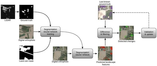
A high-level schematic of the proposed methodology for updating the landscape feature layer is shown in Figure 1. A segmentation neural network is first trained using the new DOP against the targets sampled from the last known ground truth (Figure 1 top), and the trained model is used to perform the segmentation of the whole region (Figure 1 bottom).

In both the training and final segmentation, the regions of specific land use, such as forests and intensive orchards, are masked out in order to exclude from model evaluation the vegetation that does not fall under the category of suitable woody vegetation landscape features. The obtained raster is vectorized, and features with areas smaller than 10 m² are removed following the methodology proposed in [1]. This eliminates potential leftover vegetation fragments from the filtering step, as well as individual bushes and small trees, which are not considered standalone woody vegetation landscape features. A vegetation change layer is produced next as a symmetric difference between the new layer and the last ground truth, and the area attributes are computed for the new features. The change layer is finally filtered with respect to user-specified threshold values for minimum area and percentage of change. This allows the user to focus on the most significant changes first or specify the minimum required extent of change to be registered. The changes are validated manually by visual inspection of the DOP or through field inspection before they are used to update the ground truth. In the case of CAS, such updates would be performed once per year after a new DOP is obtained for the target areas where woody vegetation landscape features are lacking owing to intensive agricultural practices.

2.2. Study Area

The selected study area is the region of Goričko, which lies between 46°61′–46°88′N and 15°98′–16°43′E, covering approximately 462 km² of hilly landscape in the northeastern-most part of Slovenia (Figure 2). It is the largest landscape park in the country (with the exception of the National parks). The region was selected because it is one of the highest priority areas for the preservation of existing and the formation of new woody vegetation landscape features in the country, and environmental actions are implemented here much more easily owing to the specific land ownership structure. The whole landscape park also falls under the Natura 2000 network of protected areas for biodiversity conservation, which makes Goričko an interesting target for continuous surveillance of agricultural practice implementations.

2.3. Data

The datasets used in this study are the LiDAR point clouds, the DOP, the building cadastre, the public infrastructure cadastre and the land use database for the selected study area of Goričko.

The LiDAR scanning of Goričko was performed in early 2014. The average density of first returns calculated over 10 m² squares was 5 points/m², while the root mean square error (RMSE) of absolute height measurements for the entire survey block was 8 cm (http://gis.arso.gov.si/related/lidar_porocila/b_24_izdelava_izdelkov.pdf, accessed on 22 May 2023). The geo-referenced and classified point clouds are available for download as a grid of 1 km² cells from the website of the Slovenian Environment Agency (http://gis.arso.gov.si/evode/profile.aspx?id=atlas_voda_Lidar@Arso&culture=en-US, accessed on 22 May 2023).

The DOPs of Goričko for the years 2014, 2016, and 2019 were used in this study. Aerial images was produced with a 25 cm ground sample distance. The orthorectification of images was performed using a 5 m photogrammetric digital terrain model (DTM) for the year 2014 and a LiDAR-based DTM with 1 m resolution for the years 2016 and 2019. The public digital orthophoto is accessible through the e-survey data portal maintained by the Surveying and Mapping Authority of the Republic of Slovenia (https://egp.gu.gov.si/egp/?lang=en, accessed on 22 May 2023).

The building cadastre is a vector layer containing approximately 1.18 million shapes that represent the ground plans of registered buildings for the whole country. The public infrastructure cadastre contains vector layers for different public infrastructure objects and networks, such as roads, railways, water supply networks, communication networks, and electric grids. In this study, the power transmission line layer was used, which contains the medial axes of transmission corridors. One of the important object attributes is the power line voltage level, which determines the required width of the corridor (ranging from 1.5 m to 40 m). The vegetation encroaching on the transmission corridors is not considered a landscape feature, as it is removed during periodic corridor maintenance. Both datasets can be obtained from the same data portal as DOP.

The last dataset is the national record of land use, which contains a vector layer with approximately 1.7 million objects. The objects are classified into 25 different types of land use based on photo-interpretation, field inspections, and third-party information. The updates to the layer correspond to the coverage of yearly CAS surveys, which include approximately one third of the national territory. The land use dataset is published on the website of the Ministry for Agriculture, Forestry and Food (https://rkg.gov.si/vstop/, accessed on 22 May 2023).

The main properties of the used datasets are summarized in

Table 1. Main properties of datasets used in the study.

Dataset	Data Type	Date	Properties
LiDAR	Point cloud	4/2014	Density: 5 pts/m2
DOP	RGB images	5/2014, 4/2016, 4/2019	Resolution: 25 cm/px
Buildings	Polygons	2020	#Features: 1.18 M
Transmission lines	Lines	2020	#Features: 319,455
Land use	Polygons	2014, 2017, 2020	#Features: 1.55 M–1.74 M

.

2.4. Data Processing

The original data were processed in order to produce the masks and layers needed in the later stages of the proposed pipeline. Individual pre-processing steps were performed using available open-source software tools and libraries for working with GIS data, which are described in the continuation.

The LiDAR point clouds were used to generate the reference layer of woody vegetation landscape features by roughly following the approach by Kokalj et al. [1]. The points already classified as ground were first used to generate a digital terrain model (DTM) at 1 m resolution, which matches the resolution used in the orthorectification of aerial images during the production of the DOP. The generated DTM was used to extract the raster canopy height model (CHM) using the pit-free method [59]. These steps were fully automated using the lidR package (https://github.com/r-lidar/lidR, accessed on 22 May 2023), which provides a set of tools and algorithms for the manipulation of airborne LiDAR data [60].

The vectorization of CHM was performed next, where only the pixels with a height above 2 m were considered. The result was subsequently filtered in order to remove all segments not corresponding to potential regions of interest (RoI). The filtering was performed by sequentially subtracting the geometry of individual masking layers from the vectorized CHM. In particular, the building cadastre, the public infrastructure layer, and the land use layer were used to respectively mask out urban areas, power line corridors, and registered special purpose areas, such as hop fields, greenhouses, vineyards, intensive orchards, forests, and water bodies. The power line corridors were derived from their axial representation by applying buffers of prescribed clearance widths depending on the voltage levels of the power lines.

In order to prevent detecting narrow strips of forest border and connected vegetation as separate landscape features due to the imprecision of the land use layer, a 10 m buffer was used to expand forest segments before filtering. In a similar way, a 2 m buffer was used for the building cadastre, and a 1 m buffer for the power lines. In contrast, the regular fields were not filtered out because this would remove most of the narrow linear vegetation along field edges, which are rarely delineated separately in the land use layer. Finally, the remaining segments with areas smaller than 10 m² were discarded, and the result was rasterized to produce the candidate target mask at a spatial resolution of 25 cm. All of the steps were performed using the QGIS (https://qgis.org/, accessed on 22 May 2023) software tool and automated with the GDAL (https://gdal.org/, accessed on 22 May 2023) library, which includes Python utilities for operations on raster and vector layers as well as conversions between different formats.

In order to reduce the fragmentation due to the many small gaps in the vegetation picked up by LiDAR, a morphological closing with a square structuring element of 3 pixels width was applied to the raster layer. The resulting target mask T was used as ground truth in the model training as well as to derive the potential vegetation changes based on the disagreement between the baseline and the model predictions. The joined mask M of areas that were filtered during the target mask preparation was also rasterized. It was used during the training to limit the calculation of segmentation loss to regions of interest as well as to perform the final filtering of the model’s predictions.

The training dataset for the segmentation neural network was built using 32 sample tiles corresponding to rectangular patches of land selected from various parts of the Goričko region. Each tile was 4000 × 4000 pixels and covered an area of 1 km². Another 8 tiles were used for the validation dataset during training, while the final 8 tiles were used for the test set (Figure 2). The plots were chosen such that the number of pixels belonging to woody vegetation landscape features represented at least 3% of the non-masked area in the tile.

The training, validation, and test samples consisted of spatially aligned parts of the DOP, land use mask M, and target mask T. The actual training samples were generated from the training tiles on the fly by cropping random subimages of size 1024 × 1024 pixels, which is the expected input dimension for the segmentation neural network. Training set augmentation was performed by flipping the extracted samples randomly in horizontal and vertical directions, each with a 50% probability. Unlike the training samples, the validation and test samples were obtained by uniform subdivision of the corresponding tiles into 4 × 4 cells with a 32 pixel overlap between neighboring images.

2.5. Segmentation Model

The core step of the proposed change detection methodology involved training a segmentation neural network, which uses the most recent DOP as an input and outputs a segmentation probability map. The last known state of woody vegetation landscape features was used as the target reference T for computing the training loss, while the combined land use mask M was used to constrain the loss computation to relevant pixels. The expectation was that training with fresh input data and the last ground truth as the target would force the model to misclassify primarily in areas of actual changes because adjusting for them would lead to a significantly higher overall training loss.

In our experiments, we used a pre-trained segmentation neural network based on the U-Net architecture (Figure 3) from the Python segmentation models package (https://github.com/qubvel/segmentation_models, accessed on 22 May 2023). The model allows the selection of several backbone neural network architectures, which have been pre-trained on the ImageNet dataset. We selected the EfficientNet backbone [61] because it provides better or comparable performance using a much smaller number of network parameters than other architectures, which allows network training on a regular desktop GPU. The fine-tuning of the U-Net model to a particular task of vegetation detection in DOP was finally performed. In order to speed up the training and reduce the space requirements, the encoding layers of U-Net can be frozen during fine-tuning, and only the decoding layers are adapted. However, we found that fine-tuning the complete stack was beneficial for performance, presumably because aerial imagery contains visual features and patterns not present in typical image datasets.

The training was implemented in Tensorflow using the Keras neural network library. The Adam optimizer with an initial learning rate $\eta ={10}^{-4}$ and default values for other parameters was used for model optimization. The output prediction of the model was a 2D probability map $\widehat{Y}$ with the same width and height as the input image. The loss function was a customized binary cross-entropy loss, which applied the mask of land use M to constrain loss contribution to non-masked pixels only. The errors made in pixels corresponding to regions of interest (i.e., woody vegetation landscape features), were weighted differently according to the following equation:

$$\mathcal{L}=-\frac{1}{|\widehat{Y}|}\sum _i(1-m_i)(w{y}_{i}log\left({\widehat{y}}_i\right)+(1-w)(1-y_i)log\left(1-{\widehat{y}}_i\right)).$$

Here, w is the weight for balancing false positive and false negative errors, and was, in our final experiments, set to 0.6 after extensive hyper-parameter tuning on a validation set. The mean loss was calculated over all pixels i in the output, where $m_i\in M$ is the corresponding mask value (1 for masked pixels), $y_i\in Y$ is the target value, and ${\widehat{y}}_i\in \widehat{Y}$ is the model prediction.

In the ideal case, re-training a model to a new DOP would not be required. However, there can be significant differences between photos from different surveys due to varying phenological stages of the target vegetation and illumination conditions. Some differences can be reduced by careful planning of flight dates, but this depends on many factors, including the weather. Alternatively, different training data augmentation techniques, such as brightness adjustment and adaptive histogram equalization, can be applied during the training of the original model in order to simulate varying environmental factors. The downside is that this may lower the model’s performance on an otherwise homogeneous training set such as the CAS, where a selected target region is typically recorded in a short time span, during which the state of vegetation foliage and weather conditions are consistent. Additionally, not all differences can be adequately simulated by data augmentation, and the model used in the previous cycle is likely overfitted to conditions present at the time of the aerial imagery capture. Due to that, either a fine-tuning of the previous network or the training of a new model from scratch is necessary. We compared different approaches in the experiments. The results demonstrated that training a new model was more efficient than fine-tuning a trained model from the previous cycle. The most likely reason is that fine-tuning cannot escape the local optimum basin of a model that was adapted to the seasonal characteristics of aerial images from the previous training cycle, although training data augmentation can help in reducing the performance gap.

2.6. Post-Processing and Filtering

The post-processing of model predictions in the change detection phase was completely automated using the GDAL library. The value of each pixel in the output image represents the probability of vegetation’s presence in the pixel. The image was first converted to binary using a probability threshold value of 0.5. The same mask M that was used during training was applied next in order to remove the areas of land use that were not compatible with the woody vegetation landscape feature definition. The images generated from subparts of the original tiles were concatenated back to form a single larger raster, and morphological closing with a 3-pixel window was applied to it. The result was vectorized, and the areas were computed for the so-obtained feature polygons. A symmetric difference was computed next, with the reference vector layer representing the last known state of woody vegetation landscape features. The land use mask was applied to the reference layer as well in order to eliminate areas whose land use designations may have changed since the last update (e.g., overgrown abandoned farmland can, after some time, be reclassified as forest). The resulting polygons corresponded to potential changes in nature, representing the locations of vegetation ingrowth or its removal. A final filtering step was performed in which the areas of the detected change polygons were computed first, as well as the ratio between the area of the change and that of the source polygon (reference or prediction). In the last step, all change polygons were removed whose area or percentage of change were below the user-specified thresholds.

2.7. Validation

The efficacy of the proposed approach was evaluated on an independent test set by human visual inspection. The test set included the DOPs and masks from the CAS years 2016 and 2019, which were used to extract separate woody vegetation change layers with respect to the reference LiDAR-based layer from 2014. The detected changes of woody vegetation landscape features were visualized and presented to the user in an overlay with the DOP 2014 and the DOP from the respective comparison year. The user was able to show or hide individual layers in order to validate the proposed changes. In this way, the user could label false positive (FP) and true positive (TP) cases of woody vegetation change by concentrating on the polygons in the generated layer. In order to expose the false negative (FN) cases, which represent the changes overlooked by the model, the user also had the ability to draw a polygon around the apparent change. Each such manually delineated polygon was clipped against the reference layer, and the area of the result was calculated. The percentage of area change for the polygon was finally calculated with respect to the polygon’s total area. The resulting feature was counted as a false negative if it passed the threshold conditions.

3. Results

The aim of the experiments was to simulate a typical scenario, which is first to train the segmentation neural network using the DOP from the selected CAS year as input and the LiDAR-based ground truth as target. The trained model was then applied to a test set, and the results were used to generate the woody vegetation landscape feature change layer. Separate experiments were performed using the training data from the CAS years 2014, 2016, and 2019. The data from 2014 were used only to evaluate the extent of agreement between the DOP-based predictions and the LiDAR-based reference targets from the same year. The target layer was not updated between consecutive experiments because the goal was to assess the degradation of the landscape feature registry when no monitoring was performed for an extended period of time.

The experiments were conducted on a computer with an AMD Ryzen 9 5900X CPU and an NVIDIA Geforce RTX 3060 GPU with 12 GB of VRAM. The operating system was Manjaro Linux kernel 6.0. The efficientnetb3 backbone was used as a feature extractor in the segmentation neural network. The training data for the network were 32 tiles of the aligned DOP, land use mask, and target mask. In each epoch, a single random training sample of size 1024 × 1024 pixels was extracted from each tile. The network was trained for 200 epochs, which took approximately one hour to complete. A separate validation set, which contained 128 samples obtained by uniform subdivision of 8 larger tiles, was used during training to record the best performing model variant. After training, the stored best model was used to perform the segmentation of a test set with another 128 samples.

Table 2. Training and test precision (P), recall (R), and $F_1$ score of models trained on DOPs from different CAS years and the LiDAR-based ground truth.

Year	Train			Test
	$\mathit{P}$	$\mathit{R}$	${\mathit{F}}_{\mathbf{1}}$	$\mathit{P}$	$\mathit{R}$	${\mathit{F}}_{\mathbf{1}}$
2014	88.3%	88.3%	88.3%	88.5%	87.3%	87.9%
2016	81.4%	83.3%	82.3%	83.6%	83.3%	83.5%
2019	6.0%	73.9%	74.9%	78.7%	75.6%	77.1%

summarizes the results in terms of the achieved per-pixel precision (P), recall (R), and $F_1$ score on the training and test sets.

As explained before, the training of a new model for each CAS cycle is desirable for the best results, because not all seasonal differences in aerial photography can be adequately simulated by data augmentation. We tested this using a series of experiments. We first used the 2014 model directly to perform the segmentation of DOP 2016 and DOP 2019, which resulted in an $F_1$ equal to 71.7% and 67.2%, respectively, a substantially worse outcome than what we got with the dedicated model. As the next step, the 2014 training data were augmented using random combinations of brightness, contrast, hue/saturation/value, and histogram equalization. The $F_1$ scores of the resulting model improved to 75.7% and 69.8%. The last attempt involved additional fine-tuning of the 2014 model with new data for 50 epochs using a smaller initial learning rate $\eta ={10}^{-5}$. This improved the $F_1$ score for the 2016 and 2019 datasets further to 81.2% and 74.9%, respectively, but the preference clearly remained for specialized models.

The two trained models for the years 2016 and 2019 were used to produce corresponding change layers for woody vegetation landscape features as described in Section 2.6. Two levels of thresholding were applied during the filtering stage in order to assess the usability of the approach at different granularities. For level 1, the more selective threshold values $T_1=100$ m² for the minimum area of change and $T_2=20\%$ for the minimum percentage of change were used in order to make the process of manual validation manageable. At level 2, the relaxed requirements $T_1=30$ m² and $T_2=10\%$ were used for comparison purposes only.

Figure 4 shows, for a selected region, the DOPs from different years, the detected landscape features, and the changes corresponding to the two filtering levels.

Table 3. Validation results for the produced landscape feature change layer at the threshold values $T_1=100$ m² and $T_2=20\%$.

Year	TP	FP	FN	P	R	F1
2016	84	30	10	0.737	0.894	0.808
2019	173	49	19	0.715	0.901	0.836

reports the number of detected changes for the case $T_1=100$ m² and $T_2=20\%$, as well as the counts of TP, FP, and FN determined by visual inspection of the results.

The high-detail change detection at level 2 resulted in 772 detected changes in 2016, and 1142 detected changes in 2019. It should be noted that, by reducing the threshold values, the increasing number of detected changes was due to the displacement of objects in orthorectified DOPs. There were also many cases where the gaps between previously sparse vegetation were overgrown. However, we considered this to be a valid case for joining previously fragmented woody vegetation landscape features into larger plots.

4. Discussion

The proposed approach to monitoring woody vegetation landscape features differs from related studies in that it addresses the complete workflow necessary to support semi-automated layer updates. A segmentation neural network is trained in order to detect woody vegetation landscape features in a DOP from periodic aerial surveys. The initial training target is generated from LiDAR point clouds, while the detected vegetation changes are presented for validation and used for subsequent database updates. Unlike the more general vegetation detection approaches, the proposed methodology uses additional layers for vegetation filtering in both the model training and the post-processing phases.

We compared the segmentation performance of our model with similar studies that used UAV [41] and high-resolution satellite images [42]. In ref. [41], a U-Net model was used for shrub segmentation, and achieved an $F_1$-score of 82% on images with a comparable spatial resolution of approximately 25 cm/pixel. This is below the 88% score of our model obtained with the contemporary DOP and reference layer. The authors reported a notable drop in performance on images with distinct seasonal characteristics, which is consistent with our findings about the use of the same model on images from different surveys. By using satellite images with a 1 m spatial resolution for mapping in woody vegetation, the approach in [42] achieved a precision and recall of around 88%, which is very close to our results. However, both reference approaches involved manual labeling of training data, while our method uses a LiDAR-based ground truth.

Based on the comparable training and test set results in Table 2, we can conclude that overfitting of the segmentation models to the training set did not occur. As demonstrated by the results, the best training performance can be achieved by training a separate model for each year of the aerial photography cycle. Besides assuring similar imaging conditions and vegetation states, an additional motivation for the use of specialized models in the case of CAS is that individual aerial surveys cover parts of the country in adjacent photogrammetric blocks where the landscape and vegetation are relatively homogeneous [62]. Indeed, in a country with highly diverse natural biotopes, an even finer granulation of models could be applied at the level of individual blocks at a reasonable additional cost of preparing separate training data. For instance, the eastern part of Slovenia is recorded in three photogrammetric blocks, which include both the Pohorje medium mountain range and the Pannonian plain. The survey of the western country part, similarly, encompasses four blocks of diverse alpine and karstic landscapes, which could benefit from sub-specialized models. Such an approach would be feasible given the low cost of model training.

Another finding of the study is that end-to-end fine-tuning of a pre-trained model is superior to training the decoder alone. This is consistent with the results of related studies, which have shown that fine-tuning of the encoder is beneficial for performance [63,64]. It was further established that transfer learning from a generic pre-trained model was more efficient than additional fine-tuning of a model from the previous cycle. Similar findings have been reported in the literature [65]. Although the surveys were made in the same period of the year, there were important year-to-year differences in the phenological stages of vegetation and capture conditions, and it was shown in [66] that such significant data distribution shifts cannot always be adequately simulated by synthetic data augmentation.

Regarding the validation of the detected changes, it can be observed from Table 3 that the number of false negatives was considerably lower than the number of false positives. A low false negative rate is desirable, since false positives are easier to discover by subsequent verification. There was, consequentially, a noticeable gap between the achieved precision and recall, owing to the model’s preference for false positives. It can also be observed that the number of detected changes grew with the increasing temporal difference between the reference and the current time. From an ecological perspective, it was interesting to analyze the trend of the detected changes. According to the validated changes, the net area loss of woody vegetation landscape features in the test plots was approximately 11.5 ares in 2016 and 15 ares in 2019, which represents roughly 2% and 3% of the corresponding landscape feature areas in 2016 and 2019, respectively. Moreover, such information is of crucial importance for agricultural policy decision-makers as well as for parcel owners who can control and, with financial support, potentially improve the detected unfavorable ecological status of the environment.

Our results demonstrate that a reliable detection of changes in woody vegetation landscape features with a true positive rate of around 90% is possible. An important insight from the experiments is how the representativeness of the reference layer deteriorates without regular updates, since the number of validated changes in the test set more than doubled between consecutive surveys (from 94 in 2016 to 192 in 2019).

The analysis of the disagreement between the LiDAR-based ground truth and the woody vegetation landscape features detected in the DOP showed that there are two main sources of false differences. The first one is radial displacement of objects in orthorectified aerial photography, which results in bands of misclassified pixels along opposing edges in woody vegetation patches. This is illustrated in Figure 5, where the woody vegetation landscape feature is identified correctly by the model but is shifted slightly with respect to the LiDAR target, indicating a change. The majority of such cases are eliminated later during the filtering step because either the area of the change or its percentage within the feature polygon is below the threshold.

The second source of mismatches between the model predictions and LiDAR targets is the ability of LiDAR to detect low vegetation, smaller clearings, and gaps, which are not included in woody vegetation landscape feature delineation. It is also able to capture finer details in woody vegetation edges, which the up-sampling part of the segmentation neural network cannot reconstruct as precisely (Figure 6). There are two possible ways to address this in future work: by using a wider window for morphological closing of targets or by incorporating edge-preserving loss in model training [67]. However, most changes detected due to such differences are typically fragmented into many smaller patches, which can be filtered by a properly set minimum area threshold.

There are some limitations to the proposed DOP-based vegetation localization that affect the efficiency of change detection. Insufficient foliage in late-sprouting vegetation in particular can cause the segmentation model to underestimate the extent of the growth and indicate a change where there was none. In order to avoid an unnecessarily high number of such false positives, the phenological stage of woody vegetation would need to be considered in determining future surveys since their initial purpose was not specifically vegetation monitoring.

A more general limitation of monitoring woody vegetation landscape features is that, from an ecological perspective, not all plant species are equally important for biodiversity. The possibility of accurately determining the species composition of small woody features from single-shot aerial photography is severely constrained. In fact, the spreading of some fast-growing invasive species is becoming a serious problem globally [13,68], and such vegetation sites should not be considered valuable landscape features. The proposed framework could also be used to indicate the potential propagation of invasive species by detecting fast-expanding growth.

5. Conclusions

In the paper, we propose a methodology for automated detection of woody vegetation landscape features in cyclic aerial photography and the construction of change layers with respect to the reference ground truth. Systematic registration and monitoring of woody vegetation is essential for the efficient implementation of ecosystem and biodiversity preservation strategies. While LiDAR and high-resolution satellite imagery are the best sources for reliable vegetation detection, their high cost makes them less suitable for continuous monitoring. As this study demonstrated, a viable solution is to utilize the remote sensing data of periodic aerial surveys, which present an attractive balance between cost and resolution required for change detection on a regional scale.

Based on the results, we can conclude that the entire end-to-end pipeline for the generation of change layers can be implemented in a way that requires almost no user intervention. The main application of such methodology is for semi-automated updates of the landscape feature registry, where the user can set the desired granularity of detected changes before they are presented for manual validation. This allows the user to focus on major disruptions first in order to make an early assessment of trends.

There are several ways the proposed methodology could be improved in the future. In the segmentation stage, a better precision in detecting feature boundaries could be achieved by extending the loss function, or employing specialized neural network architectures. In the post-processing stage, the number of false positives could be reduced by explicit matching of overlapping shapes, i.e., detected and reference woody vegetation landscape features. The filtering thresholds could also be adjusted locally by using the canopy height model to estimate the possible amount of radial displacement due to orthorectification. These improvements would increase the precision of change detection without sacrificing recall, leading to an overall improved user experience.

From the end-user perspective, an important extension of the proposed workflow would include visual analytics in order to facilitate the supervision of how the national strategies for biodiversity and nature preservation are implemented. The proposed methodology can be used in a similar way to monitor other interesting types of habitats for ecological monitoring, such as meadows or marshes. Locating areas of fast vegetation expansion could also be used to indicate the potential progression of invasive species. Another possible application of the proposed approach is in planning and overseeing long-term periodic field operations, such as vegetation maintenance in transmission line corridors.