Article

Developing Spatial and Temporal Continuous Fractional Vegetation Cover Based on Landsat and Sentinel-2 Data with a Deep Learning Approach

1
Hubei Provincial Key Laboratory for Geographical Process Analysis and Simulation, Central China Normal University, Wuhan 430079, China
2
College of Urban and Environmental Sciences, Central China Normal University, Wuhan 430079, China
3
School of Remote Sensing and Information Engineering, Wuhan University, Wuhan 430079, China
*
Author to whom correspondence should be addressed.
Remote Sens. 2023, 15(11), 2948; https://doi.org/10.3390/rs15112948
Submission received: 10 April 2023 / Revised: 27 April 2023 / Accepted: 3 June 2023 / Published: 5 June 2023

Abstract

:
Fractional vegetation cover (FVC) has a significant role in indicating changes in ecosystems and is useful for simulating growth processes and modeling land surfaces. The fine-resolution FVC products represent detailed vegetation cover information within fine grids. However, the long revisit cycle of satellites with fine-resolution sensors and cloud contamination has resulted in poor spatial and temporal continuity. In this study, we propose to derive a spatially and temporally continuous FVC dataset by comparing multiple methods, including the data-fusion method (STARFM), curve-fitting reconstruction (S-G filtering), and deep learning prediction (Bi-LSTM). By combining Landsat and Sentinel-2 data, the integrated FVC was used to construct the initial input of fine-resolution FVC with gaps. The results showed that the FVC of gaps were estimated and time-series FVC was reconstructed. The Bi-LSTM method was the most effective and achieved the highest accuracy (R2 = 0.857), followed by the data-fusion method (R2 = 0.709) and curve-fitting method (R2 = 0.705), and the optimal time step was 3. The inclusion of relevant variables in the Bi-LSTM model, including LAI, albedo, and FAPAR derived from coarse-resolution products, further reduced the RMSE from 5.022 to 2.797. By applying the optimized Bi-LSTM model to Hubei Province, a time series 30 m FVC dataset was generated, characterized by a spatial and temporal continuity. In terms of the major vegetation types in Hubei (e.g., evergreen and deciduous forests, grass, and cropland), the seasonal trends as well as the spatial details were captured by the reconstructed 30 m FVC. It was concluded that the proposed method was applicable to reconstruct the time-series FVC over a large spatial scale, and the produced fine-resolution dataset can support the data needed by many Earth system science studies.

1. Introduction

Vegetation is an essential component of Earth’s terrestrial ecosystems, since it serves as a bridge connecting the soil, water, and atmosphere. Forest carbon sinks are an important potential solution for global climate change, and the absorption of carbon dioxide can be enhanced by protecting and restoring vegetation [1]. Therefore, it is vital to obtain high-resolution and real-time information on vegetation cover. When monitoring the dynamics of the Earth’s vegetation, fractional vegetation cover (FVC) can be used to quantify the surface vegetation. The FVC is the percentage of the vertical projection area of green vegetation on the ground to the total statistical area [2]. The temporal dynamics of FVC are a useful indicator for environmental changes, such as drought and extreme wet conditions, and are an accurate indicator of the start of the growing season [3]. Additionally, this time series can be utilized to compare vegetation status in agriculture and forestry from year to year [4]. Therefore, FVC is an essential candidate for replacing classical vegetation indices for monitoring green vegetation [5]. To date, several methods have been proposed to estimate the FVC. Typically, these methods are divided into three major categories: empirical-based, physical-model-based, and spectral- unmixing-based [6].
With the rapid development and popularization of remote sensing technology, satellite data present continuous improvements in the detection range, temporal coverage, and spatial and temporal resolution [7]. Large-scale dynamic vegetation monitoring technology is becoming increasingly mature and is very suitable for the rapid estimation of vegetation coverage and understanding of the dynamic changes in global vegetation coverage [8]. Many institutions around the world have obtained FVC products using various retrieval methods based on satellite data (e.g., MERIS, SPOT, and POLDER) [9,10,11]. Current global-scale FVC products have been generated using remotely sensed data with medium spatial resolution, including VGT bioGEOphysical product Version 2 (GEOV2), Copernicus Global Land Operations (CGLOPS), and Global Land Surface Satellite (GLASS) FVC products [12,13,14]. However, there is an increasing demand for fine data applications. This means that FVC products based on low- or medium-spatial-resolution satellite data are not adequate to address the current demand for vegetation analysis. Meanwhile, owing to low spatial resolution, it is difficult to capture the precise spatial distribution of vegetation in highly heterogeneous and complex terrains. As a result, vegetation information extraction is less accurate.
With the continuous improvement of satellite sensors and computing capabilities, high spatial resolution satellites, such as Landsat, Sentinel, and GF, have been widely used for various quantitative remote sensing studies [15]. Several studies have used these satellites as data sources, combined with different retrieval methods, to obtain fine-resolution FVC products. The MuSyQ GF-series FVC product used Gaofen-1 satellite data to generate FVC with 16 m/10 d resolution in China from 2018 to 2020. However, this FVC product has only been available for 3 years in China, restricting time-series analysis [16]. To assess the usefulness of the hyperspectral imager (HSI) onboard the Chinese HJ-1-A small satellite for vegetation mapping, Zhang et al. [17] used dimidiate pixel models to retrieve 100 m FVC in the Shihezi Area of Xinjiang, China. The retrieved 100 m FVC from the HJ-1/HIS data was consistent with the in situ measurements with an R2 of 0.86 and RMSE of 10.9%, indicating that HJ-1/HSI data can provide fine-scale monitoring of vegetation cover changes. Ludwig et al. [18] generated 10 m/7 d resolution of woody vegetation cover for the Molopo region in 2016 based on Sentinel-1 and Sentinel-2 data. Gill et al. [19] used Landsat 5 TM and Landsat 7 ETM+ data with a spectral unmixing approach to generate woody vegetation cover data for Australia from 2000 to 2010 at 30 m resolution. In addition, the data had a coefficient of determination of R2 = 0.918, as verified by field measurements. In summary, despite the expanding number of fine-resolution FVC products from regional to national scales, most FVC models only estimate fine-resolution FVC for small or medium-sized regions, and the short period of the estimated FVC is still not conducive to large-scale, long-term vegetation analysis.
The Landsat-based FVC product is a global FVC product with 30 m resolution and long time series, using Landsat data as its data source and selecting training samples from Landsat 8 and Gao Fen 2 based on the Random Forest (RF) algorithm [20]. The Landsat FVC product outperforms other FVC products in terms of spatial resolution. This makes it more effective in investigating vegetation cover in small areas by providing finer details of the distribution of vegetation cover and allowing for the long-term monitoring of vegetation dynamics in recent decades. However, there are several issues with Landsat FVC products. Given that Landsat satellites revisit every 16 days, the Landsat FVC is frequently discontinuous in time series and is often contaminated by clouds or high concentrations of aerosols, resulting in fluctuations or gaps in the FVC product. In addition, certain areas are cloudy all year round, making it difficult for Landsat satellites to obtain accurate observations in these areas. As a result, they often have long periods of missing data, causing the vegetation cover data to be incomplete and discontinuous in both temporal and spatial aspects. Therefore, there is an urgent need to reconstruct the Landsat FVC to improve its spatial integrity and temporal continuity.
To fill in the gaps between the missing dates and cloud occlusion in the fine-resolution FVC, we attempt to reconstruct the time-series FVC spatially and temporally. Currently, the most effective method of achieving such objectives is through the integration of multi-source spatial resolution data, referring to other vegetation time-series parameters, and using deep learning methods. Additionally, there has been much research on the spatio-temporal reconstruction of satellite data products. For example, Chen et al. [21] obtained high-quality interpolated reconstructions of missing time in time-series images by fitting synthetic NDVI time series produced by combining MODIS NDVI data with Landsat cloud-free observations using a Savitzky–Golay (S-G) filter. Gao et al. first proposed the Spatial and Temporal Adaptive Reflectance Fusion Model (STARFM), which improves remote sensing data by fusing high-resolution Landsat data with low- and medium-resolution MODIS data [22]. The Flexible Spatio-temporal Data Fusion (FSDAF) method was proposed by Zhu et al. based on spectral unmixing analysis and a thin plate spline interpolator [23]. Morteza used the FSDAF algorithm to produce Landsat-like land surface temperature images with Landsat spatial and MODIS temporal resolutions [24]. Zhou fused MODIS and Landsat data to generate time-series NDVI and EVI with 30 m spatial resolution for dryland vegetation monitoring in Qinghai Province [25]. Walker fused MODIS and Landsat data to generate a 30 m spatial resolution time series of NDVI and EVI for dryland vegetation monitoring in Arizona [26]. Meng combined NDVI from HJ-1 CCD and MODIS for crop biomass estimation [27].
In recent years, deep learning methods have been widely applied in various remote sensing estimation applications and have outperformed traditional machine learning methods. Among the many deep learning architectures, recurrent neural networks (RNNs) can address the time dependence of time-series data [28] and handle time-series regression or prediction of satellite data. In vegetation index estimation based on time-series data, this approach has excellent noise tolerance and nonlinear processing ability, which can solve the limitation problem when data saturation exists. For instance, the reconstruction of high-quality NDVI time-series data was achieved using Long Short-Term Memory (LSTM) and the predictive reconstruction of MODIS NDVI time-series data, the results of which were well adapted to NDVI series trends [29]. Perceptual layer neural networks were used to extract vegetation cover from randomly selected training samples [30]. The LSTM deep learning framework was applied to spatio-temporal environmental dataset prediction based on experimental results from three marine datasets [31].
In this study, we aim to optimize the spatio-temporal integrity of FVC results and produce an accurate fine-scale vegetation dataset at a regional scale. All Sentinel-2 and Landsat 8 observations within a single year were integrated to derive the 30 m FVC, which contained gaps, at least twice a month. We compared three common reconstruction methods by applying them to the incomplete 30 m FVC. We selected the method with the highest accuracy at sample sites and optimized the method in terms of the model input and parameters to satisfy a regional application. Finally, the optimized method was selected and applied to produce the 30 m/16 d FVC of the study region.

2. Study Area and Materials
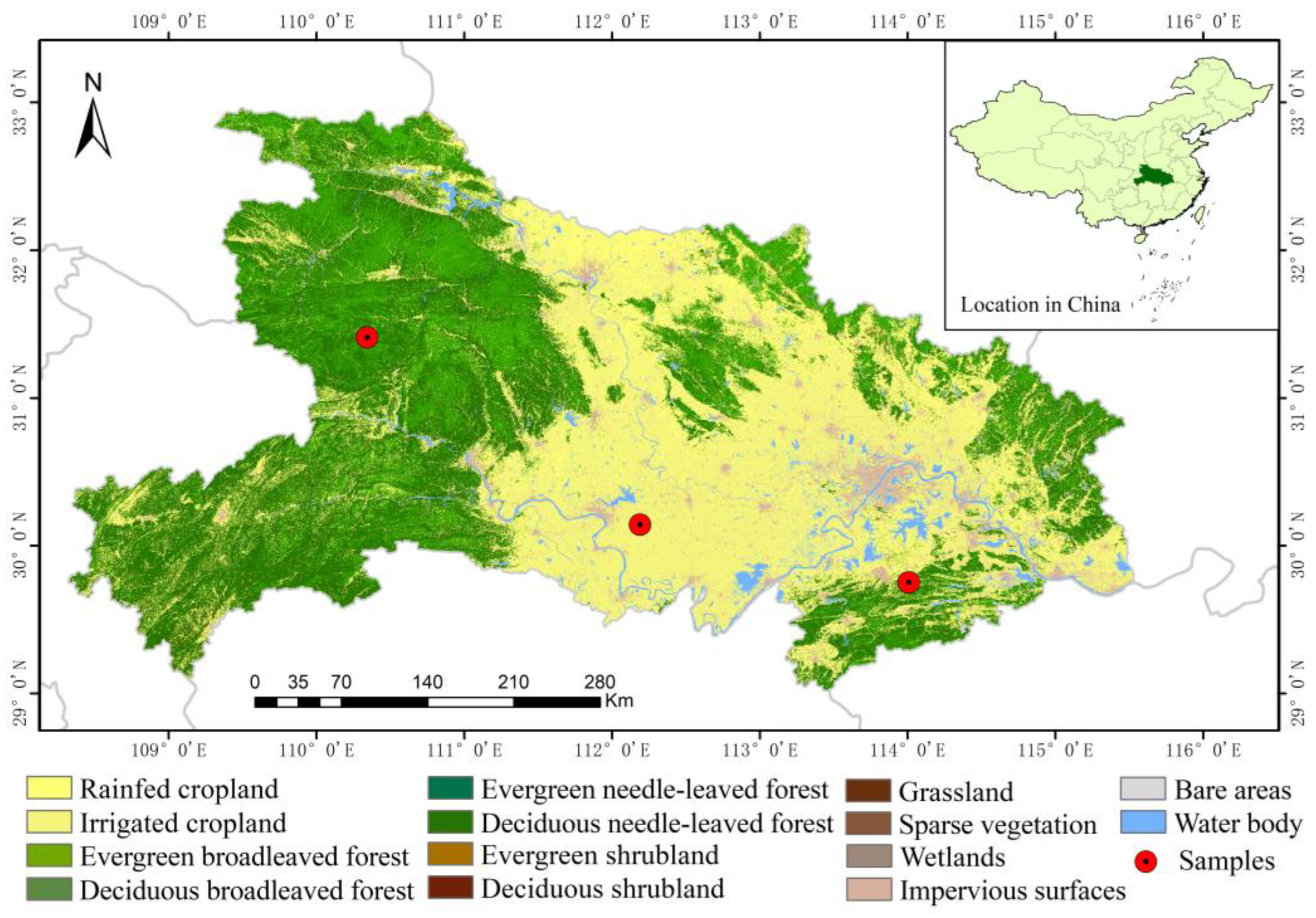
2.1. Study Area

Hubei Province is located in the middle Yangtze River basin of central China, and it includes the Jianghan Plain for cropland. The vegetation cover types in Hubei are mainly deciduous and evergreen forests and croplands. To compare the accuracy of different reconstruction methods, we selected three sample sites in Hubei Province representing different types of vegetation (Figure 1). The method with the highest accuracy was further applied to the entire province for regional analysis.

2.2. Fine-Resolution Satellite Data and Preprocessing

2.2.1. Landsat 8 Data and Preprocessing

Launched in February 2013, the Operational Land Imager (OLI) sensor is a high spatial resolution multi-spectral imager onboard the Landsat 8 satellite in a sun-synchronous orbit (705 km altitude) with a 16-day repeat cycle. Landsat 8 data are suitable for pixel-level time-series analysis [32]. Thus, using Landsat surface reflectance data as the data source, the Landsat FVC product was developed based on the RF algorithm to select training samples. Landsat FVC has a spatial resolution of 30 m on a global scale and a temporal resolution of 16 d, covering the period from 2013 to the present [20]. In this study, we used 27 Landsat 8 images acquired in 2017 covering 3 sample sites to test reconstruction methods and 129 images covering the entire province for regional FVC retrieval.

2.2.2. Sentinel-2 Data and Preprocessing

The Sentinel-2A/B product available for users is Level-1C data (https://scihub.copernicus.eu, accessed on 1 October 2022), which refers to top-of-atmosphere reflectance in cartographic geometry in the UTM/WGS84 projection, with a size of 100 km × 100 km. The study area was covered by one Sentinel-2 tile (T49RGP). Sentinel-2 L1C data covering 2016 to 2018 in the study area with less than 10% cloud cover was used. Sentinel-based FVC data were generated using the RF model.
Sentinel-based FVC was generated in two steps: preprocessing and FVC estimation. The preprocessing of the Sentinel-2 data included atmospheric correction, spatial resampling, BRDF normalization, and band normalization. The European Space Agency (ESA) recommends free, open-source Sentinel Application Platform (SNAP) toolboxes developed by the ESA for the scientific exploitation of Sentinel-based information. The Sen2Cor algorithm in the SNAP toolbox, version 2.4.0, was utilized for atmospheric correction. It eliminated the effects of the atmosphere and delivered the Level-2A product, which is a bottom-of-atmosphere reflectance in cartographic geometry. Band-pass normalization was used to reduce the small difference between the spectral bands of MSI and OLI sensors [33]. Next, the preprocessed Sentinel-2 images were used as input to produce the FVC using the same RF model as the Landsat FVC [20]. In this case, we manually selected 61 Sentinel-2 tiles acquired in 2017, covering the 3 sample sites, as the data source to produce the original fine-resolution FVC. For regional analysis, 548 Sentinel-2 tiles were utilized.

2.3. Coarse-Resolution Satellite Products

CGLOPS produced a global 300 m resolution FVC product (FCover 300) by applying a dedicated neural network to instantaneous top-of-canopy reflectance from Sentinel-3 OLCI (v1.1 products) and daily top-of-aerosol input reflectance from PROBA-V (v1.0) from 2014 to the present (https://land.copernicus.eu/global/products/fcover, accessed on 1 October 2022). The GEOV2 (v2.0) FVC product was derived through the Geoland2/BioPar project from SPOT/VEGETATION (SPOT/VGT) and PROBA-V (GEOV2/PV) observations at 1 km and a 10 d step, extending the temporal coverage of global FVC from 1981 to the present. The FVC estimated from PROBA-V was based on neural networks [12].
GLASS products include Leaf area index (LAI), Fraction of Absorbed Photosynthetically Active Radiation (FAPAR), Broadband Albedo (albedo), Broadband Emissivity (BBE), Land Surface Temperature (LST), Daily Net Radiation (NR), Evapotranspiration (ET), Gross Primary Production (GPP), Net Primary Production (NPP), and Air Temperature (AT). GLASS products have been demonstrated to be of high quality and accuracy and are widely used [34]. This study used data from each GLASS product from 2016 to 2018 and selected GLASS products with similar (no more than three days) dates to the Landsat-based and Sentinel-based FVC data as training samples. Furthermore, we resampled the resolution of each GLASS product uniformly to 1 km as multivariate features were added during the deep learning training.

3. Methodology

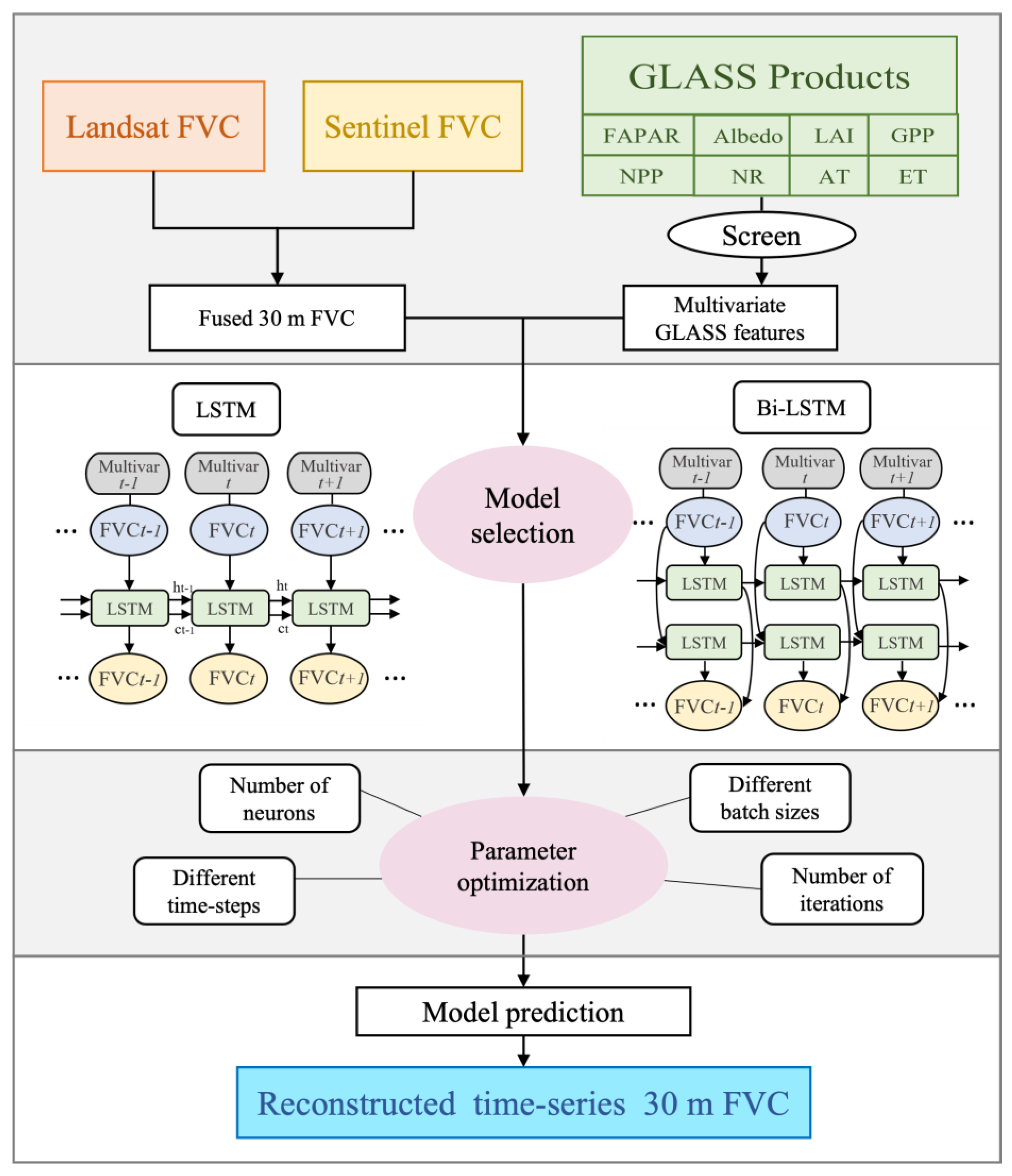
3.1. Research Framework

In this study, the spatio-temporal reconstruction of fine-resolution FVC was based on data fusion, time-series fitting, and a deep learning approach. These methods were evaluated to identify the most efficient methods for spatio-temporal reconstruction. A schematic overview of the reconstruction approach is illustrated in Figure 2, which includes three key steps. First, the preprocessed Sentinel-2 data were used to generate the Sentinel-2-based FVC using the RF model. Then, Landsat and Sentinel FVC images with a 30 m spatial resolution were reconstructed by applying different spatial and temporal reconstruction methods. These included STARFM, S-G filtering, and different LSTM models with changing variables. Finally, the accuracy of the predicted FVC was estimated, and the advantages and disadvantages of these three methods were assessed. The predicted results were consolidated at a resolution of 30 m to reconstruct the 30 m FVC.

3.2. Reconstructing FVC Using STARFM

To optimize the temporal continuity of 30 m FVC, we used the Spatial and Temporal Adaptive Reflectance Fusion Model (STARFM) algorithm [22] to combine a pair of coarse- and fine-resolution images at moment t1 and coarse-resolution image data at the moment t2 and simulated and predicted the fine-resolution image data at the moment t2 with different spatial weights. The formula is as follows:
L x w 2 , y w 2 , t 2 = i = 1 w j = 1 w k = 1 n w i j k × M x i , y i , t 2 + L x i , y i , t 1 M x i , y i , t 1
where (xw/2, yw/2, t2) represents the central pixel to be predicted by the moving window at the moment t2, w is the size of the moving window, wijk is the weight factor of pixels in the window similar to the central pixel, and L and M denote the pixel values of the fine-resolution image and the coarse-resolution image, respectively. The fusion method predicted the target pixel using the uniqueness of the spectrum, uniqueness of time, and relative distance between neighboring pixels and the target pixel. This was incorporated to give weight to the central pixel value at the moment of prediction. The FVC data in this study were input into the model with a window size set to 25. Additionally, pixels with spectral similarity to the central pixel FVC were sought in the 30 m FVC data based on spectral correlation and then combined with different weights and conversion coefficients to calculate the predicted value of the central pixel.
Here, using a subset of T49RGP as an example, the full year 2017 was used for this study, with 7 tiles of Landsat FVC, 14 tiles of Sentinel FVC, and 36 tiles of FCover 300 (1 tile every 10 d, from 1 January 2017, to 31 December 2017). After normalizing the DN values and ensuring that the two pairs of images cover the same spatial extent, we used Landsat FVC products based on Landsat and Sentinel-2 (30 m) as the fine-resolution image data and FCover (300 m) as the coarse-resolution image data to predict the FVC values in a particular region on a particular day.

3.3. Reconstructing FVC Using S-G Filtering Method

The S-G filtering method, also known as the data-smoothing polynomial filtering method, is a convolution algorithm based on smoothed time-series data and the principle of least-squares [35]. The algorithm can be described as follows:
Y j * = i = m m C i × Y j + i N
where Y j * is the fitted value, Y j + i is the original value of the image element, Ci is the coefficient when the first i value is filtered, m is the width of the filter window, and N is the filter length, which is equal to the width of the sliding array, 2m + 1. In practice, S-G filtering requires two parameters to be set: the filter window and the order of polynomial operations. Based on the characteristics of the S-G filter, setting a filter window length that is too small may overfit the data points, making it difficult to capture the trend of the entire time series. However, setting a filter window length that is too large may miss some significant changes in the FVC time series. Different polynomial orders can also affect the fitting results of the S-G filter, and this parameter is generally set from two to four.
Considering the importance of temporal details in the FVC time series for phenology studies, we conducted a study with different combinations of w and d and finally chose a parameter combination of w = 7 and d = 2. This parameter choice provides an excellent trade-off between retaining temporal variation details and the overall time-series trend. Considering the edge effect seen in the S-G filter, the 0 m FVC during the period from December 2016 to January 2018 was employed to constitute a complete filter window for the first four points and the last four points of the NDVI time series. To evaluate the performance of the S-G filter, a subset of the T49RGP (113°37′–113°43′E, 29°43′–29°48′N) was used to construct a high-quality FVC time-series dataset.
Here, using Sentinel-based and Landsat-based FVC as input, we filled in the time series of FVC at 30 m resolution. A total of 31 scenes of the T49RGP from 2017 were selected as the time series. They were entered into the S-G filter model for spatio-temporal reconstruction. As the data were processed using Fmask4.0, the empty values caused by clouds and shadows were flagged as no values. Thus, we could reconstruct the data values in the image directly. Additionally, for scenes with missing dates, the entire scene was reconstructed as if it were all no-data values.

3.4. Reconstructing FVC with LSTM and Optimized Parameters

3.4.1. The LSTM Method

Time-series data prediction refers to learning patterns of change in past time series and predicting future trends. Traditional deep learning methods are unable to solve the problem of change over time, which has resulted in the development of RNNs. However, because RNNs perform poorly in solving long-term-dependent information, Hochreiter et al. proposed LSTM by adding the structure of gates to the RNN to selectively add or remove time-series information [36]. The LSTM cell states consist of two activation functions (sigmoid and tanh), which constitute the forgetting, input, and output gates. The sigmoid function outputs the input parameters as values between 0 and 1. These values are used to determine the impact on the model, with a maximum impact of 1. The tanh function outputs the input parameters as values between −1 and 1, which are used to normalize the results.

3.4.2. The Bi-LSTM Method

Bi-LSTM is another alternative RNN containing two separate recurrent net layers: forward and backward layers [37]. Bi-LSTM combines the strengths of RNNs and LSTM by applying LSTM-gated memory units to a bidirectional propagation model. The Bi-LSTM network has the advantage of using information from the entire input time-series sequence when predicting the current target, effectively solving the disadvantage that LSTM can use only information from the previous moment. Figure 3 illustrates LSTM and Bi-LSTM structures. Where Ct represents the long-term memory of the cell, ht represents the short-term memory of the unit, and FVCt represents the external input. It can be seen that Ct passes through each cell by deleting unimportant information and adding relevant information thereafter. In general, short-term memory, which is used as the final prediction, is the result of the interaction between Ct, ht-1, and FVCt-1.
To build the dataset for model training, the corresponding 2016 to 2018 time-series 30 m FVC data from the study area were extracted as training data. Owing to the small training set, the dropout method was used to randomly remove neurons during the learning process to prevent overfitting. The time interval of the training data for the input model was set to 16 d. Additionally, the masking layer incorporated the missing dates into the model to automatically skip them during training. This was to ensure that the dataset for the training model had the same time interval.
In this study, LSTM and Bi-LSTM were used to train the model. These two methods were designed as one input layer, one LSTM/Bi-LSTM layer, one masking layer, one dropout layer, and one output layer. The LSTM and Bi-LSTM models were trained using Landsat and Sentinel-based FVC time-series data. The ratio of the training set to the test set was 7:3.

3.4.3. Changing the Time Steps

To investigate the impact of the LSTM model’s time step on reconstruction performance, we conducted separate experiments comparing single and multiple time steps. The single-step prediction (one-to-one) model takes the previous time step as input and predicts the next subsequent value in the time series, while the multi-step prediction (many-to-one) produces a predicted output using multiple inputs from the previous time steps. By comparing the estimated R2 and RMSE performance of the one-step (1SP) and multi-step (3SP) models, we can determine which time step scheme yields the best performance.

3.4.4. The Inclusion of Various Input Variables

Furthermore, it was found that LSTM based on multiple feature inputs can improve prediction accuracy [38]; whereas, we currently only use FVC as a single variable to predict the model. In this study, we added GLASS products as multivariate data to the original model for multivariate LSTM prediction. We conducted statistical analyses of the data for the different factors for which GLASS products were selected as multiple variables. Based on the results of the analysis, we removed factors with low or insignificant trends from the time series. We retained factors with a high correlation with FVC. Univariate and multivariate models with different factors were trained separately, and their accuracies were compared. Here, we selected GLASS product data from 2016 to 2018, and the date of each product was kept consistent with the date of the FVC training data. Ideally, the difference in timepoints should not exceed three days. In addition, to simplify the calculation and training, we resampled all GLASS products at a spatial resolution of 1 km. To compare different GLASS variables, we employed the Phik (φk) coefficient, a new and practical correlation coefficient proposed by Baak et al. [39]. It is a practical correlation coefficient based on refinements to the Pearson correlation coefficient, which captures the nonlinear dependency, and is useful when measuring the correlation of different variables.

3.5. Validation of the Reconstructed FVC

Whether the FVC generated by spatio-temporal reconstruction can accurately and truly reflect the missing data of Landsat FVC needs to be confirmed by validity analysis. In this study, three approaches were adopted: (1) First, we used visual verification of the consistency of the spatial distribution at the image level. (2) Second, assuming the real date FVC as the missing date FVC to be predicted, the results predicted by the three methods were compared with the real FVC in a scatter plot. The closer the distribution of points in the scatter plot is to a 1:1 line, the less variability in the spatial distribution, and the more accurate the prediction. The validation of the results was further tested by comparing the fitting of the prediction results of the different methods with the true values of the time-series curves. (3) Third, we compared the reconstructed FVC with the available FVC product in the time-series curves to verify its consistency with the reference FVC.
To evaluate the accuracy of each method, we used the R2 and RMSE values calculated based on the real FVC and predicted FVC. These values were calculated using the following equations:
R ² = 1 i ( F V C i _ p r e d F V C i _ r e a l ) ² i ( F V C i _ p r e d F V C i _ a v e r ) ²
R M S E = 1 n u m _ p i ( F V C i _ p r e d F V C i _ r e a l ) ²
where i is the number of testing samples; FVCi_pred and FVCi_real denote the predicted and real FVC for sample i, respectively; and FVCi_aver is the average of all FVC predictions.

4. Results

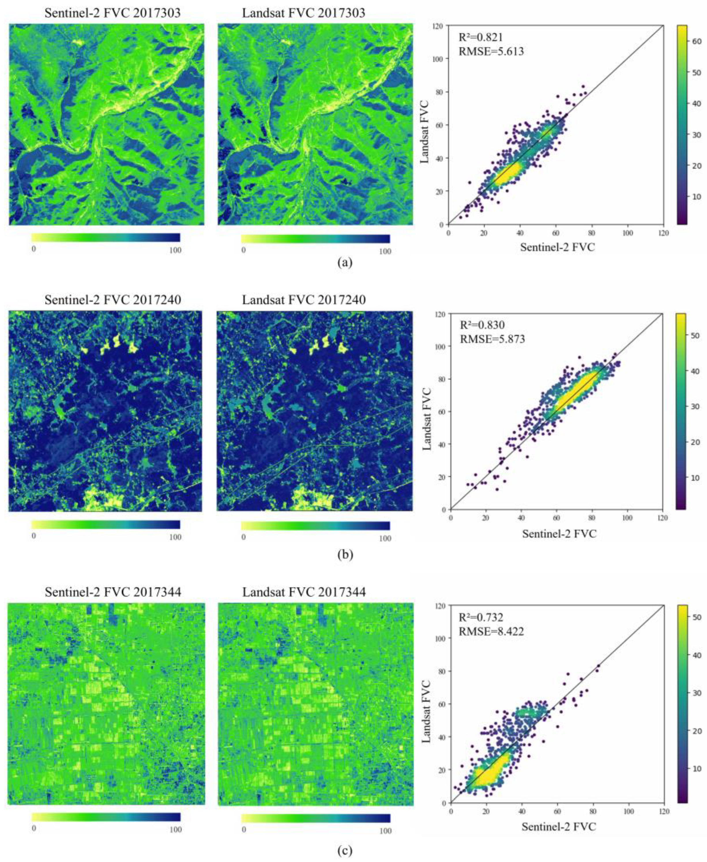
4.1. Consistency between the Landsat and Sentinel-2 FVC

The comparison between the Sentinel-based and Landsat-based FVC is shown in Figure 4 in terms of image level and scatter plot over various vegetation cover types. The correlation was 0.83 for the summer woodland (Figure 4a) and 0.82 for grassland (Figure 4b). The high correlation between the two FVCs indicates that Landsat and Sentinel-2 FVCs were overall consistent after band normalizations. The Landsat FVC had slightly higher values than the Sentinel-2 FVC, likely due to terrain effects in mountainous regions. The overall FVC values were lower than for cropland. In Figure 4c, the window was mainly featured with rainfed and irrigated cropland, and the FVC values were concentrated within the lower ranges (10–30%). The overall correlation was 0.732, which is slightly lower than other vegetation types. The Sentinel-2 FVC was slightly lower than the Landsat FVC. The points that deviated from the 1:1 line were possibly owing to residues in the band normalization and uncertain FVC values for cropland. At the image level, the Landsat-based and Sentinel-based FVCs have similar spatial distributions across different vegetation types. The results demonstrated that the combination of FVC from Landsat and Sentinel-2 can be used as input to reconstruct the time-series 30 m FVC.

4.2. Comparison of Different Reconstruction Methods

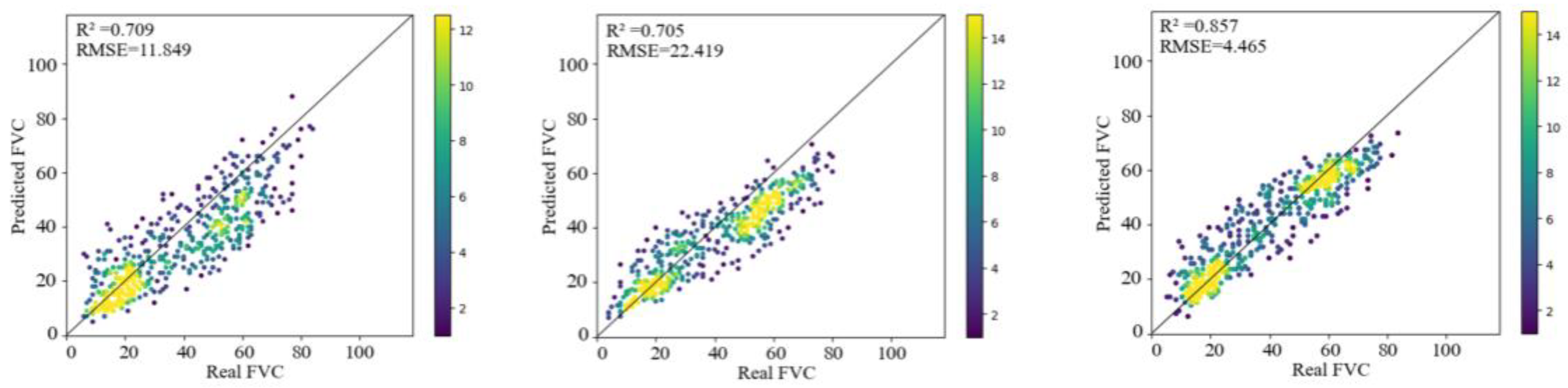
4.2.1. Accuracy Comparison of Different FVC Reconstructions

The results of the comparison between the real and predicted FVC values are illustrated for a subset of the data located in T49RGP. The scene located in this subset was mainly composed of cropland and evergreen broad-leaved forests. Visually, the reconstruction results predicted by the three methods presented similar overall spatial distributions to the real FVC values, successfully capturing the details of the FVC variations (Figure 5). While there were unrealistic areas in all the strategies, the LSTM method generated the most reliable prediction. The distinction between low and high FVC values in the STARFM results was not as clear as that in the other methods. This was especially true in forested and non-forested areas, because STARFM uses coarse spatial resolution FVC as reference data and cannot accurately distinguish vegetation from non-vegetation. Both the S-G filter results and the STARFM results underestimated high FVC values to varying extents, while the LSTM results showed improved predictions for high FVC values, but slightly overestimated low FVC values, such as bare soil and cropland in the northwest of the subset and forest in the north.
To further evaluate the performances of these three strategies, we verified the prediction results by comparing the scatter plot with real data. Overall, the pixel-to-pixel validations showed significant consistency between the real and predicted FVC values (Figure 6). In terms of prediction accuracy, LSTM (R2 = 0.857) performed better than STARFM (R2 = 0.709) and S-G (R2 = 0.705). Compared with the S-G filter and LSTM, STARFM had more points distributed far from the 1:1 reference line, and more points appeared to be biased. The dense distribution of points in the LSTM results in a low-value range of 10 to 30. Additionally, the high-value range of 50 to 70 indicates that the LSTM was able to effectively distinguish between high and low values. This characteristic was also found in the S-G filter results, where the points were more densely distributed in both intervals (Figure 6). However, the points in the STARFM results were less sensitive to the high-value range than the other two methods (Figure 6), probably because of the incorporation of coarse-resolution data.

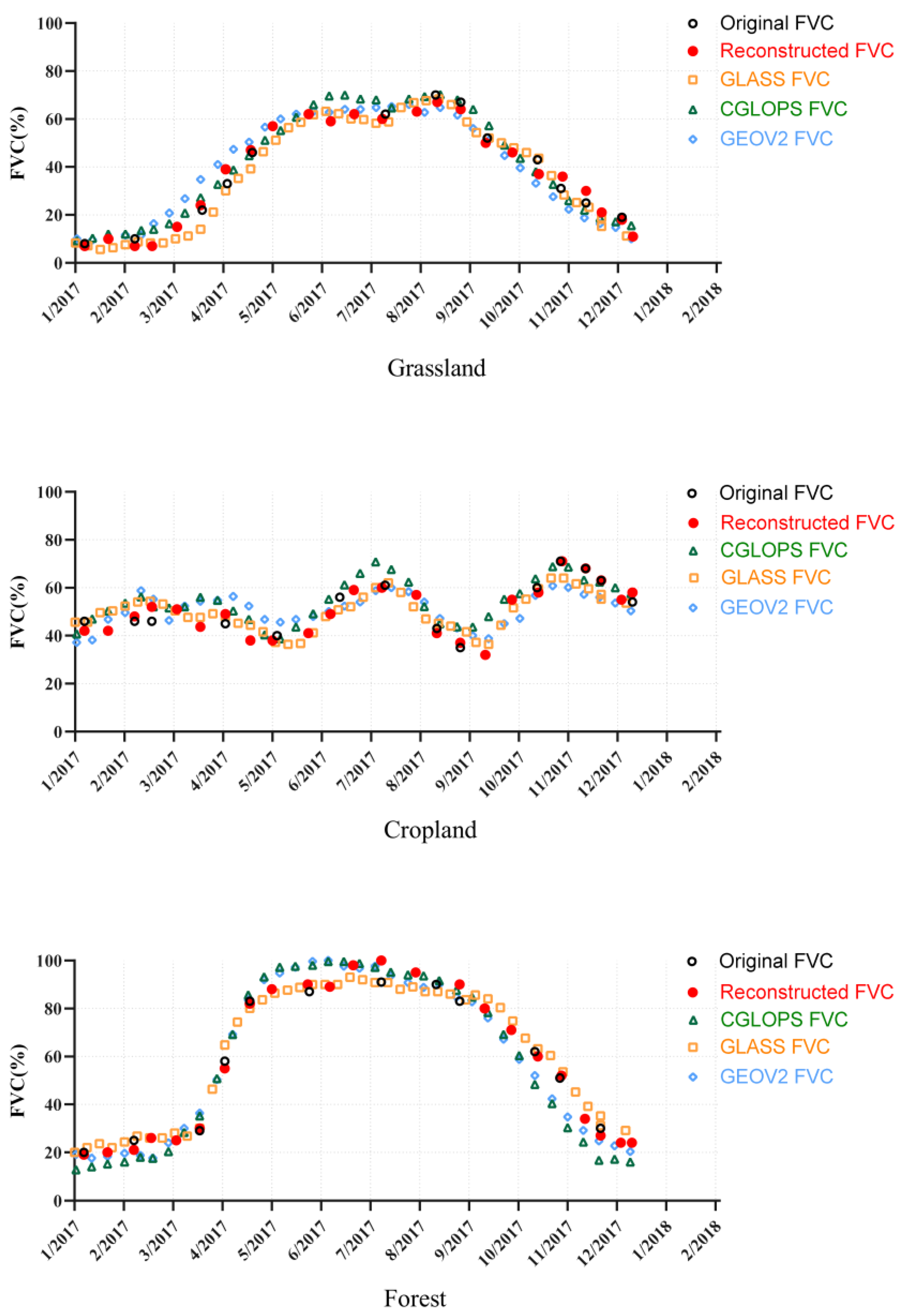
4.2.2. Time-Series FVC Derived from Different Reconstruction Methods

We performed spatio-temporal reconstructions on different samples using three reconstruction strategies. In the results of the consistency analysis of the FVC time series of randomly selected pixels (Figure 7), the black line represents the time series of the real FVC data, and the other three colors represent the time series of the results obtained using different time reconstruction methods. The overall fitting results of the three methods reflected the normal growth conditions and seasonal change patterns of the vegetation. Among them, LSTM had the most accurate fit (RMSE = 8.175), followed by STARFM (RMSE = 19.628) and S-G filtering (RMSE = 22.857). The results of the small subset spatio-temporal reconstruction indicated that all three strategies were effective in reconstructing the FVC time series.
Additionally, FVCs reconstructed from three methods are capable of revealing the annual variation and phenological characteristics of various vegetation types. The temporal resolution of the reconstruction results was improved. In addition, the number of reconstructed images increased owing to the integration of the STARFM method with the 10 d resolution FCover FVC data. However, there were several abruptly changing values in the STARFM reconstructions (e.g., April, 15, 19 July and 10 October), which may be partially due to the quality of the referenced coarse-resolution data and may also be due to differences in satellite images before and after crop harvest. The reconstructed results of the S-G filtering method were solely based on Sentinel FVC and Landsat FVC as inputs, without other reference data. Therefore, the S-G filter is limited by the original time-series data, and the prediction results may be affected by the absence of the original data. The Bi-LSTM deep learning model runs more slowly than the other two algorithms but solves the problem of noise (contamination from clouds and snow) or missing values contained in the FVC data more efficiently than other methods. This is because Bi-LSTM can effectively extract information from the entire FVC time series, rather than a single point in time, which means that the Bi-LSTM model enables us to capture the dependencies of the FVC time sequence data and predict the missing or future FVC values with high accuracy.

4.3. Accuracies of LSTM Models with Changing Parameters

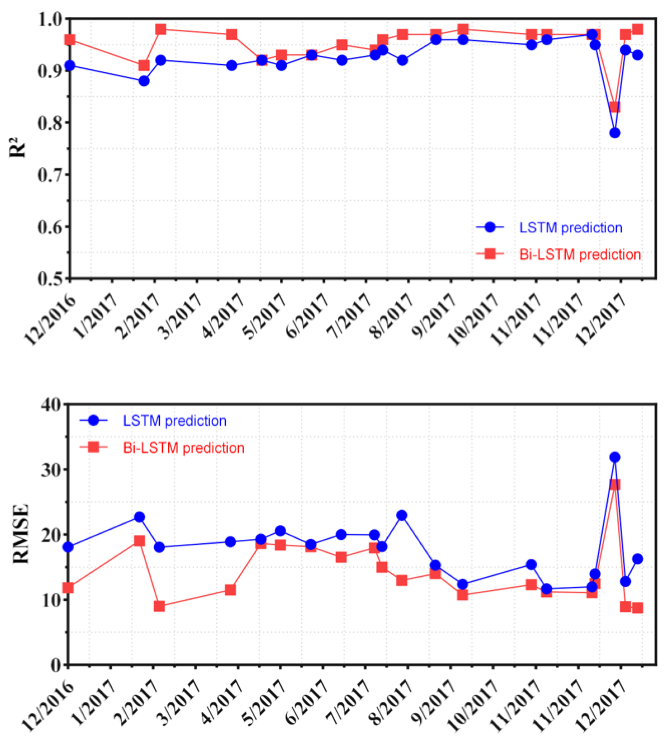
4.3.1. Accuracies of LSTM and Bi-LSTM

The performance of the deep learning model in reconstructing the 30 m time-series FVC was assessed using two metrics, the R2 and RMSE. We trained the deep learning model using an I80V598 desktop computer (Intel i7, 4 CPU, RX550 GPU, 3.6 GHz, 24 GB RAM). To obtain the optimal parameters, we performed a tuning experiment. The results showed that the model predicted accurately when the number of neurons was 128 and the number of iterations was 2000. We trained both the LSTM and Bi-LSTM models with the training dataset separately, and the training results showed that Bi-LSTM performed more effectively, as assessed by both R2 and RMSE (Figure 8). This is because the Bi-LSTM model can use information from the entire input time series when predicting the current target, effectively solving the drawback that traditional LSTM can only use information from the previous moment.

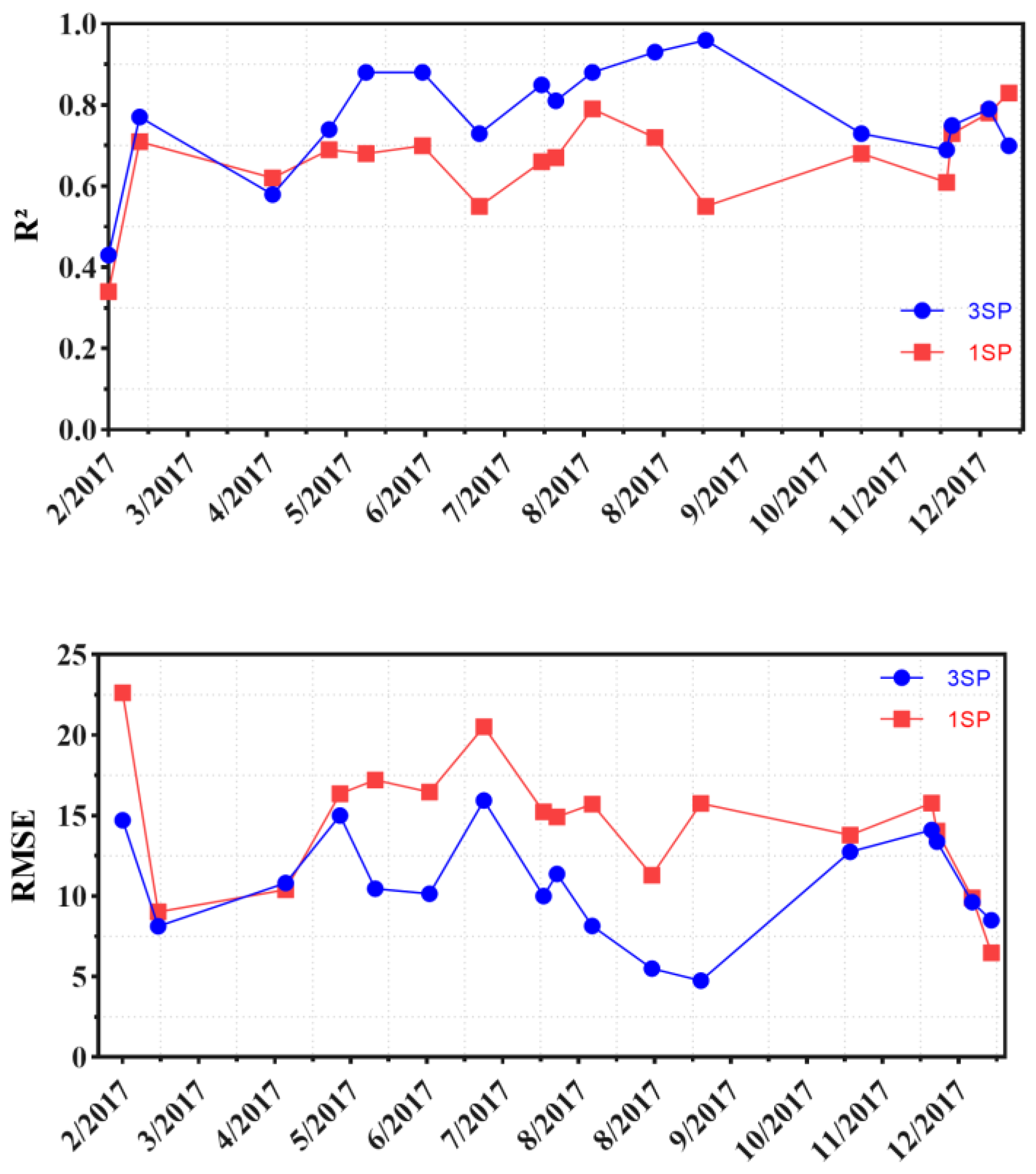
4.3.2. Accuracy of Changing the Time Step

A comparison of the prediction results with different time steps (Figure 9) shows that the prediction results using three time steps (3SP) were more accurate than the prediction results with a single time step (1SP). This is because single-step prediction is based on the most recent data and cannot be applied across input or output time steps, whereas multistep prediction is based on multiple data points and has more temporal dependency characteristics.

4.3.3. Accuracy of Changing Input Variables

According to the statistical results of the Phik (φk) correlation coefficient (Figure 10), FAPAR, Albedo, LAI, GPP, and NPP were highly correlated (here, GPP and NPP were re-moved because the same vegetation indices were used for GPP, NPP, and FVC), indicating that they can be used as training features for multivariate analysis. We trained the LSTM neural network based on different features. A comparison of the training results (Table 1) shows that the accuracy of the model with GLASS LAI data added is higher than that of the original model. However, this was not the case when there were more variables. When variables such as LAI, Albedo, FAPAR, AT, ET, NR, BBE, and LST were added to the model as multivariate features, model accuracy decreased. The model accuracy was highest when LAI, Albedo, and FAPAR were selected as multivariate features, in accordance with the correlation results.

4.4. Reconstructed Time-Series FVC in Hubei Using the Optimized Model

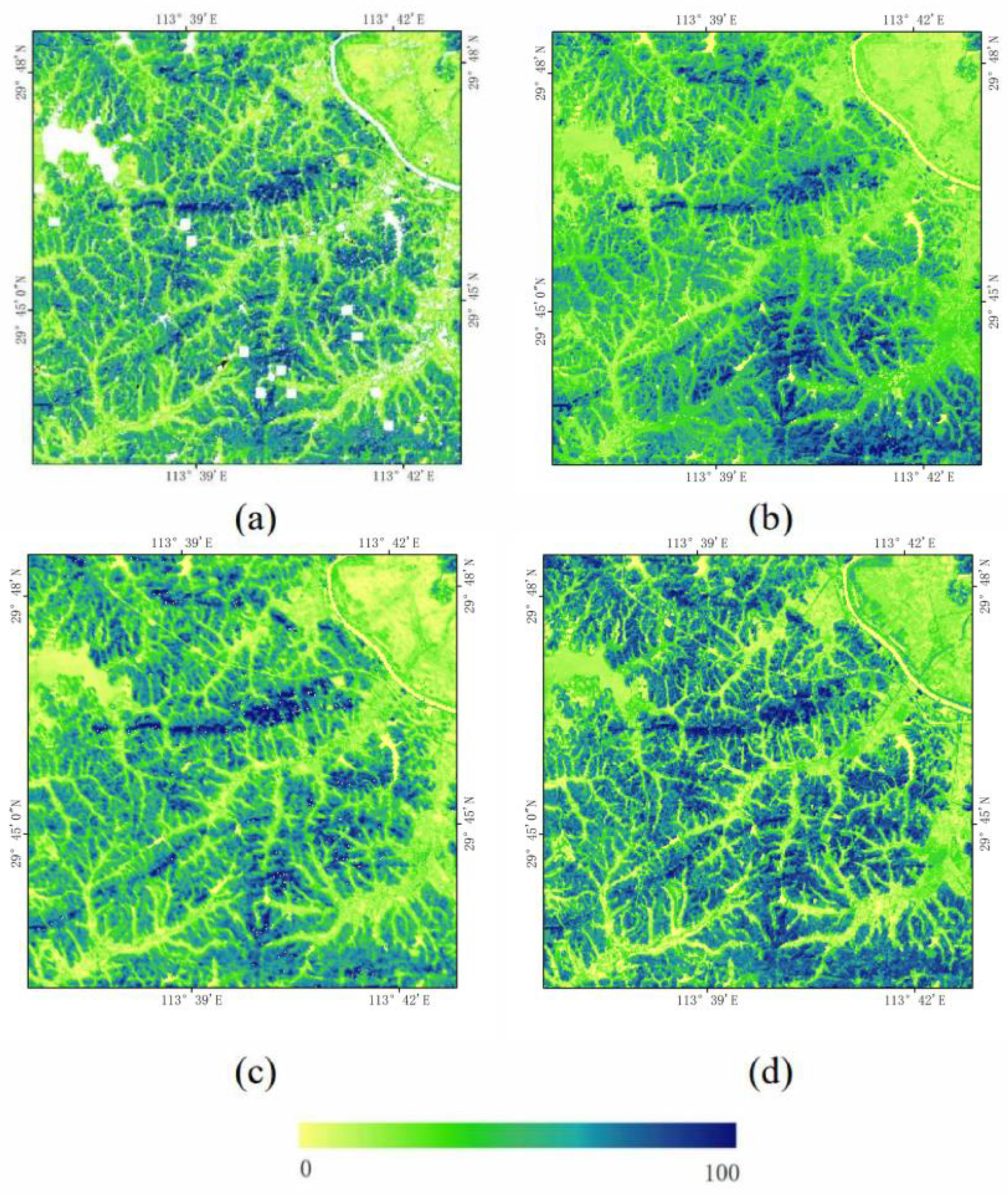
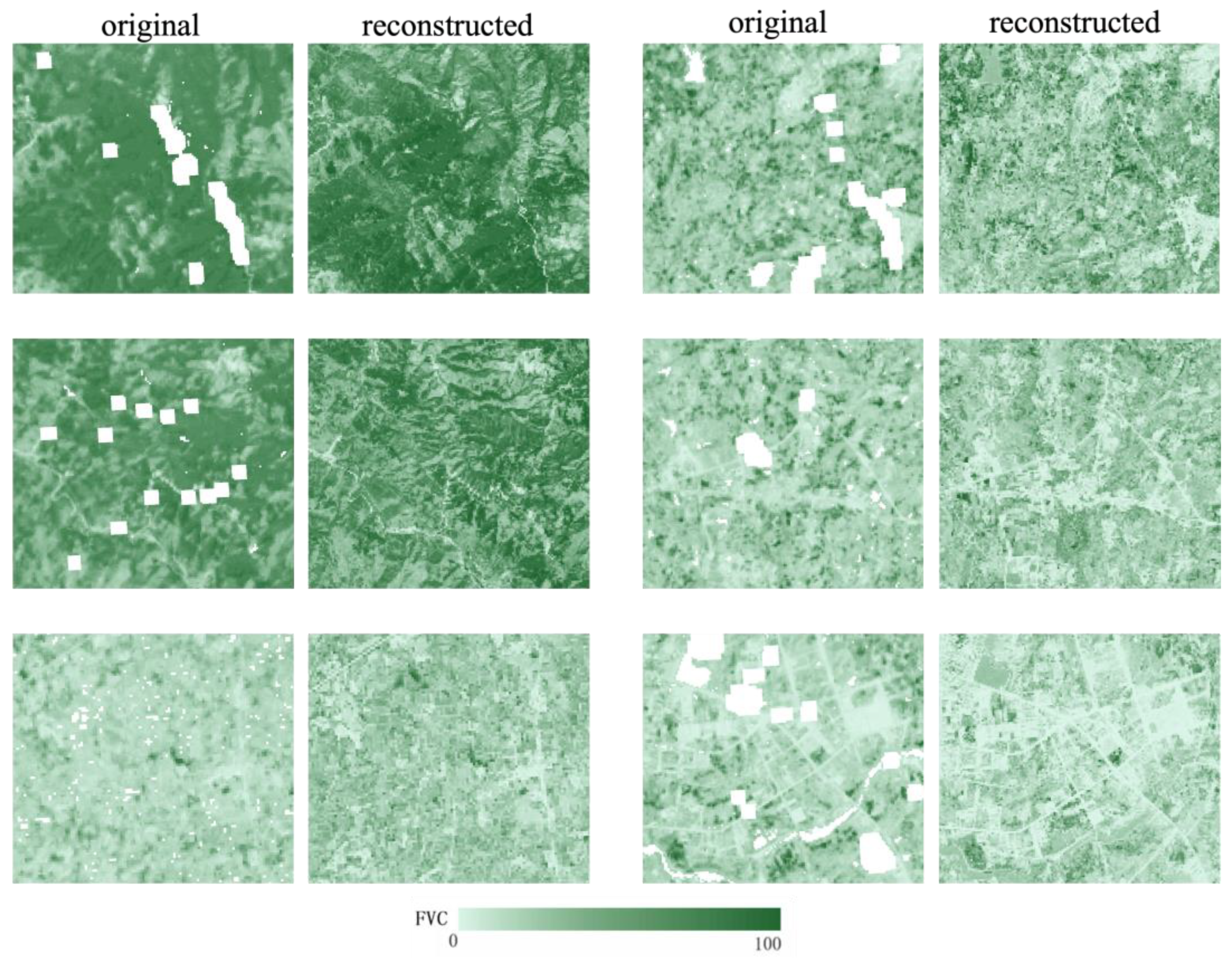
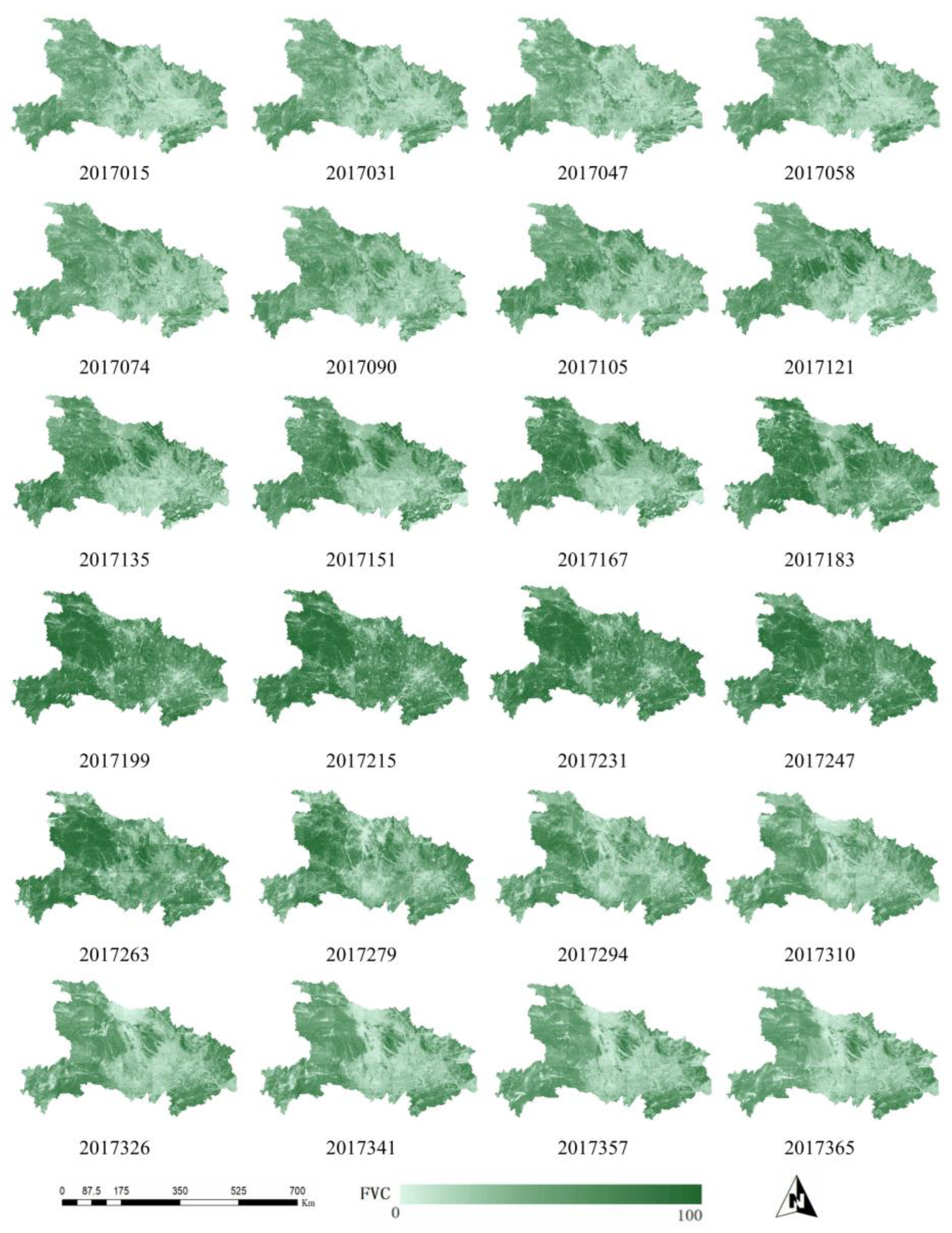
4.4.1. Spatial Performance of the Reconstructed FVC Image

In the spatial domain, the proposed method successfully reconstructed FVC values of gap pixels over different landscapes (Figure 11). The optimized Bi-LSTM model rebuilt the spatial characteristics omitted in gaps by learning from fine-resolution images at neighboring dates. The spatial details, such as roads, terrain ridges, and field boundaries, were presented in the reconstructed images. By contrast, the original FVC values were substituted by the model estimation derived from FVCs at forward and backward dates, as well as the temporal trends of coarse-resolution products. Thus, the similarity between neighboring pixels of the reconstructed images was reduced in comparison to the original images.

4.4.2. Temporal Trend of the Reconstructed FVC Pixels

At the pixel level, the reconstructed 30 m FVC differentiated seasonal trends of different vegetation types (Figure 12). Although grassland and forest pixels corresponded to a single growing season per year, the peak FVC of forests was higher than that of other vegetation types. Double cropping and single cropping were both practiced in Hubei Province in 2017 [40], as captured by the reconstructed FVC (Figure 12). The seasonal trends showed that FVC at fine resolution was close to that captured by coarse-resolution FVC products and characterized by similar start- and end-of-season dates (Figure 12). The peak occurred in July, likely owing to grasses being restored between double cropping periods [40]. Regarding the three major vegetation types in Hubei, the 30 m FVC values were usually closer to GLASS FVC, which was lower than CGLOPS and GEOV2 FVC during the growing season and higher than CGLOPS and GEOV2 FVC from November to March. Furthermore, the reconstructed FVC values of grass and forest pixels fluctuated during the peak growing periods, which was likely caused by the difference between Landsat and Sentinel-2 FVC, as well as the fluctuating trends introduced by the coarse-resolution products used in the reconstruction model.

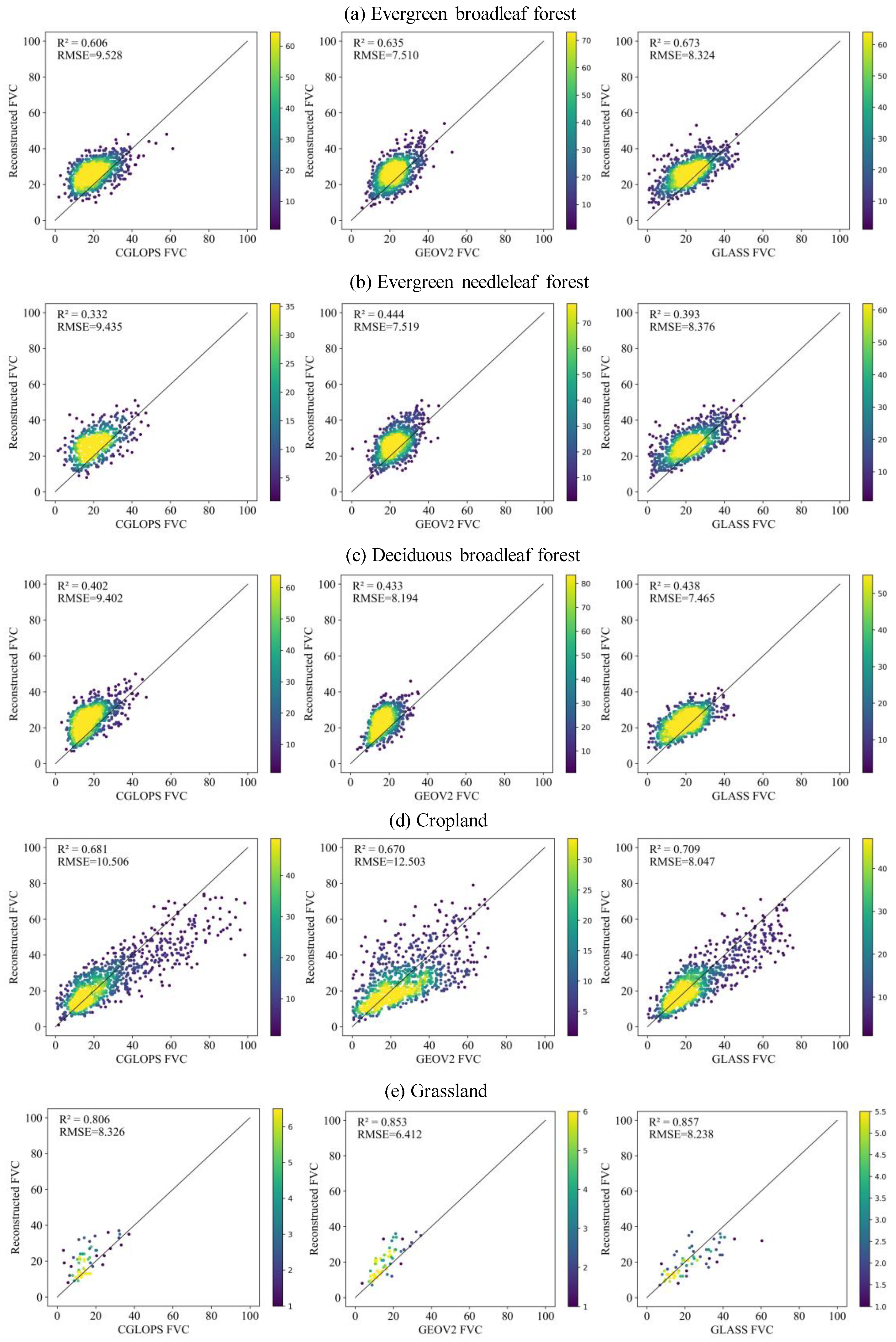
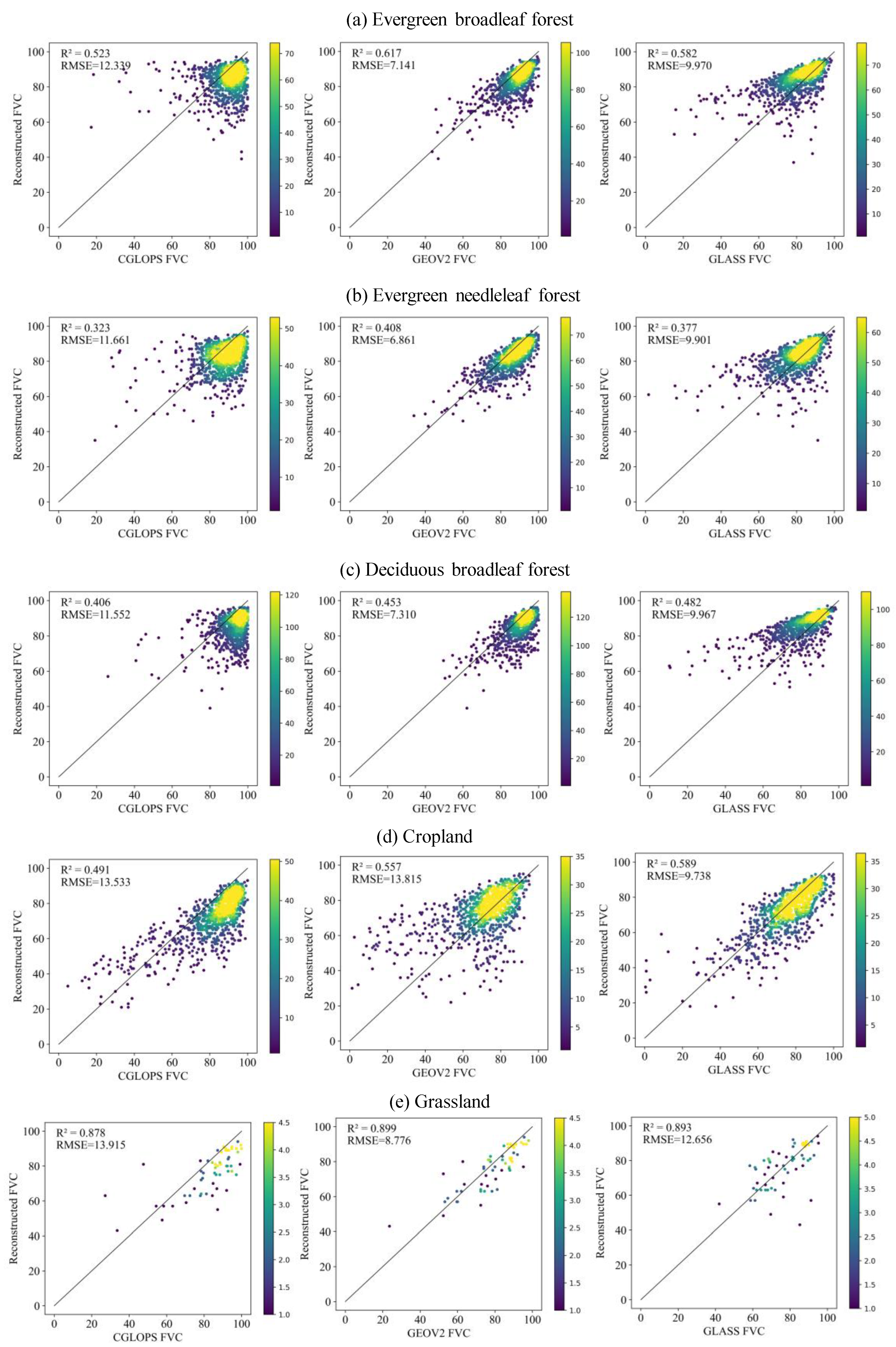
4.4.3. Regional Accuracy of the Reconstructed FVC

The 30 m/16 d FVC time series of Hubei Province in 2017 was reconstructed using the optimized Bi-LSTM model. From the reconstruction results, the FVC mosaics in Hubei illustrated spatial and seasonal variations of different vegetation covers (Figure 13). The forests located in the west of the province usually have much higher FVCs than croplands in central regions. The contrast shrank until the middle of the year, when crops, especially rice, cotton, maize, etc., were at their peak growing stages and had high FVCs. The reconstructed FVC and three reference FVC products, including GLASS, GEOV2, and CGLOPS FVC, showed a high degree of consistency across different vegetation types. Statistically, the R2 ranged from 0.4 to 0.8 and the RMSEs were generally less than 10 (FVC values ranged from 0 to 100). The R2 for cropland (0.670–0.709) and grassland (0.806–0.857) was higher than that for broadleaf forest (0.402–0.673), and needleleaf forest had the lowest R2 (0.332–0.444). The R2 and RMSE were stable for forests; however, the R2 decreased rapidly from 0.70 to 0.589 for crops from January (Figure 14) to July (Figure 15). This is likely because different types of crops were in different growing stages in July, causing uncertainties in FVC estimations for crops. The reconstructed FVC presented the highest consistency with the GLASS FVC product for both seasons and vegetation types (Figure 14 and Figure 15). This suggests that the reconstructed FVC can effectively capture information on seasonal changes in various vegetation types. As a result, the time-series FVC reconstruction of the region demonstrates the feasibility of the proposed method for rebuilding a 30 m spatial resolution FVC at a larger scale.

5. Discussion

5.1. Implications of the Reconstructed 30 m FVC Dataset

Current FVC products, such as the GEOV2, GLASS, and CGLOPS, are usually generated at a spatial resolution of several hundred meters [12,13,14], enabling the large-scale analysis of vegetation dynamics while hindering the investigation in heterogenous landscapes. The Landsat FVC provides global long time-series FVC datasets at a 30 m spatial resolution [20], but it suffers from spatial incompleteness and temporal discontinuity caused by cloud cover and a long revisit cycle. To overcome these limitations and improve the efficiency of utilizing 30 m FVC imagery, this study compared different reconstruction methods and proposed a deep learning based method to develop 30 m FVC products. The reconstructed FVC dataset is complete in a spatial extent and continuous with a time interval of ~16 d. The reconstructed 30 m FVC in Hubei Province can greatly improve the current understanding of spatial and temporal dynamics of vegetation in vital ecological regions, which previously was derived from coarse-resolution products [41]. By applying the proposed reconstruction method to the entire Landsat 8 FVC, a time-series, 16 d FVC dataset can be derived for the past decade. Such a fine-resolution dataset is highly desired by researchers from the field of urban plant phenology, who address vegetation characteristics and changes caused by long-term urbanization processes in complex urban landscapes [42,43].

5.2. Uncertainties of Different Spatio-Temporal Reconstruction Methods

Each of the three reconstruction methods had advantages and limitations. When using the STARFM model for prediction, the combination of the spatial resolution of Landsat FVC and the temporal resolution of CGLOPS FVC allows the reconstruction results to reflect the dynamic changes in vegetation growth with high accuracy. Owing to the difference in temporal resolution between the reference data and the original 30 m FVC data, there may be a bias of several days in the selection of matched images, which is one of the reasons for the uncertainty in the reconstruction results. Coarse-resolution data cannot accurately distinguish vegetation and non-vegetation on the surface, causing the STARFM predictions to fail to distinguish between high and low FVC values. In addition, the reconstruction of the STARFM method is highly dependent on coarse-resolution reference data; without reference data, the STARFM method cannot make predictions. However, a more effective ESTARFM algorithm is available [44]. Given the small amount of raw data and large date interval, which does not effectively provide input data for both time pairs, the ESTARFM algorithm was not chosen for the reconstruction.
The uncertainty of the S-G filter reconstruction results is mainly embodied in the time interval of the input data, which can adversely affect reconstruction accuracy. In the case of long date intervals especially, S-G filters are unable to fit the time-series curve well since there are too few points in the raw time-series data input [35]. Therefore, the method is limited by the original time-series data; when the original data contains more gaps and poor time continuity, the S-G filtering method is no longer applicable. The overall accuracy of the first two models was slightly inferior compared to that of the deep learning methods. However, they have advantages such as being simple and easy to implement, having low computational complexity, high productivity, not requiring sample selection or training, and direct dependency of the accuracy of the model reconstruction on the quality of the original data. Other methods, such as the FSDAF [23] and GF-SG [21], can be utilized to test the accuracy of the FVC reconstruction.
Bi-LSTM reconstructions are the most accurate method for addressing noise and missing values in FVC data, such as contamination from clouds and shadows. This is because the Bi-LSTM network can efficiently extract information from the entire FVC time series and accurately predict missing or future FVC values with high precision [45]. Furthermore, the time efficiency of training is twice that of traditional LSTM. In this study, the training samples of the Bi-LSTM model were primarily pixels of various vegetation types (mainly evergreen broad-leaved forests and croplands) in tile T49RGP; therefore, the representativeness of the training samples and the transferability of the training model still need to be improved. To avoid the use of the Convolutional LSTM for image processing specifically, it was discovered that using the Convolutional LSTM would destroy the original spatial distribution structure of the surface vegetation because of the heterogeneity of the reconstructed regional surface. During future research, we hope to expand the sample area to provide a more representative sample for training LSTM models. In addition, we intend to use in situ weather station measurements (e.g., temperature and precipitation) as training features for multivariate LSTM models. Deep learning methods also have many advantages in large-scale and multi-temporal FVC mapping. These advantages can be summarized as follows: (1) the model can achieve spatio-temporal reconstruction with higher accuracy without using auxiliary data when making predictions; (2) the neural network model can ensure that the reconstruction interval is fixed, which means that the LSTM model can reconstruct high-accuracy FVC even during long periods of poor data quality or no observational data.

5.3. Further Improvements to the Proposed Method

In this study, the Sentinel-based FVC was produced using the RF model proposed by Song [20]. By comparing the FVC images under three typical vegetation covers, the consistency of the FVC produced by the two different sensors was verified. However, the model was trained using Landsat data, and despite the normalization operation, some differences were observed between the data obtained from the two sensors. In addition, when the GLASS product data were added to the Bi-LSTM model as multiple variables, we resampled each GLASS product to a spatial resolution of 1 km to simplify the computation, rather than one variable value per pixel, as should be the case in theory, which may be a source of uncertainty. In the future, we expect to use other parameters as multivariate training features to train the Bi-LSTM, aiming to ensure that it can capture more long-term and short-term time-dependent information and make the prediction model more robust. Furthermore, owing to differences in the temporal resolution of the sensors, all data cannot be obtained at the same time. This can lead to uncertainty during the model training and validation of the comparison. Owing to the lack of ground measurement data, the FVC in this study can only be compared with existing FVC products for accuracy verification. The reference FVC products (GLASS FVC, CGLOPS FVC, GEOV2 FVC) were selected based on their spatial coverage, time span, and spatio-temporal resolution, as well as the availability of data. However, these products have different spatial resolutions; therefore, the resolution was uniformly resampled to 300 m in the comparison, which may lead to uncertainty in the verification results [46]. While the Bi-LSTM model can produce smooth and continuous spatio-temporal predictions, the smoothing of noise in the time series may classify important ecological changes and disturbances as noise and filter them out, creating uncertainty [45]. Further research is needed to investigate how rapidly and abruptly changing FVC values may affect the model performance.

6. Conclusions

In this study, we compared three types of spatio-temporal reconstruction methods by applying them to the 30 m resolution FVC derived from integrated use of Landsat 8 and Sentinel 2 data. Among the three methods, the Bi-LSTM model was the most effective and had the highest accuracy, followed by the STARFM method and the S-G filtering method. In comparison to the data fusion and filtering method, the deep learning Bi-LSTM model captures the dependencies of the FVC time sequence data and can predict missing or future FVC values with high accuracy. Setting the proper time step in Bi-LSTM and inclusions of relevant variables, such as LAI and albedo, have further improved the prediction accuracy. Moreover, a 30 m FVC dataset of every 16 days in Hubei Province of China was produced using the optimized Bi-LSTM method. The derived time-series FVC dataset has shown the tremendous details of the spatial distribution of FVC values as well as the seasonal dynamics of different vegetation types in Hubei. It is concluded that the proposed model can effectively accomplish reconstruction of fine-resolution FVC in a province or larger spatial scale, and the generated 30 m FVC product can support many Earth system science studies.

Author Contributions

Conceptualization, D.-X.S. and T.H.; methodology, D.-X.S. and Z.W.; validation, Z.W., D.-X.S., J.L., C.W. and D.Z.; formal analysis, Z.W. and D.-X.S.; writing—original draft preparation, Z.W. and D.-X.S.; writing—review and editing, D.-X.S. and T.H. All authors have read and agreed to the published version of the manuscript.

Funding

This research was funded by the National Key Research and Development Program of China [2022YFB3903502], the National Natural Science Foundation of China [42271404], the Fundamental Research Funds for the Central Universities [CCNU22QN018], and the Natural Science Foundation of Hubei [2021CFA082].

Data Availability Statement

Not applicable.

Conflicts of Interest

The authors declare no conflict of interest. The funders had no role in the design of the study; in the collection, analyses, or interpretation of data; in the writing of the manuscript; or in the decision to publish the results.

References

  1. Huang, L.; Chen, K.F.; Zhou, M. Climate change and carbon sink: A bibliometric analysis. Environ. Sci. Pollut. Res. 2020, 27, 8740–8758. [Google Scholar] [CrossRef] [PubMed]
  2. Jia, K.; Liang, S.; Wei, X.; Yao, Y.; Yang, L.; Zhang, X.; Liu, D. Validation of Global LAnd Surface Satellite (GLASS) fractional vegetation cover product from MODIS data in an agricultural region. Remote Sens. Lett. 2018, 9, 847–856. [Google Scholar] [CrossRef]
  3. Sha, Z.; Bai, Y.; Li, R.; Lan, H.; Zhang, X.; Li, J.; Liu, X.; Chang, S.; Xie, Y. The global carbon sink potential of terrestrial vegetation can be increased substantially by optimal land management. Commun. Earth Environ. 2022, 3, 8. [Google Scholar] [CrossRef]
  4. Gao, L.; Wang, X.; Johnson, B.A.; Tian, Q.; Wang, Y.; Verrelst, J.; Mu, X.; Gu, X. Remote sensing algorithms for estimation of fractional vegetation cover using pure vegetation index values: A review. ISPRS J. Photogramm. Remote Sens. 2020, 159, 364–377. [Google Scholar] [CrossRef] [PubMed]
  5. Jia, K.; Yang, L.; Liang, S.; Xiao, Z.; Zhao, X.; Yao, Y.; Zhang, X.; Jiang, B.; Liu, D. Long-Term Global Land Surface Satellite (GLASS) Fractional Vegetation Cover Product Derived from MODIS and AVHRR Data. IEEE Trans. Geosci. Remote Sens. 2019, 12, 508–518. [Google Scholar]
  6. Jia, K.; Liang, S.; Gu, X.; Baret, F.; Wei, X.; Wang, X.; Yao, Y.; Yang, L.; Li, Y. Fractional vegetation cover estimation algorithm for Chinese GF-1 wide field view data. Remote Sens. Environ. 2016, 177, 184–191. [Google Scholar] [CrossRef]
  7. North, P.R.J. Estimation of f(APAR), LAI, and vegetation fractional cover from ATSR-2 imagery. Remote Sens. Environ. 2002, 80, 114–121. [Google Scholar] [CrossRef]
  8. Baret, F.; Weiss, M.; Lacaze, R.; Camacho, F.; Makhmara, H.; Pacholcyzk, P.; Smets, B. GEOV1: LAI and FAPAR essential climate variables and FCOVER global time series capitalizing over existing products. Part1: Principles of development and production. Remote Sens. Environ. 2013, 137, 299–309. [Google Scholar] [CrossRef]
  9. García-Haro, F.J.; Camacho, F.; Meliá, J. Inter-comparison of SEVIRI/MSG and MERIS/ENVISAT biophysical products over Europe and Africa. In MERIS/(A)ATSR User Workshop, 2nd ed.; ESA SP-666: Frascati, Italy, 2008. [Google Scholar]
  10. Roujean, J.L.; Lacaze, R. Global mapping of vegetation parameters from POLDER multiangular measurements for studies of surface-atmosphere interactions: A pragmatic method and its validation. J. Geophys. Res.-Atmos. 2002, 107, ACL-6. [Google Scholar] [CrossRef]
  11. Fillol, E.; Baret, F.; Weiss, M.; Dedieu, G.; Demarez, V.; Gouaux, P.; Ducrot, D. Cover fraction estimation from high resolution SPOT HRV&HRG and medium resolution SPOTVEGETATION sensors, Validation and comparison over South-West France. In Second Recent Advances in Quantitative Remote Sensing Symposium; Publicacions de la Universitat de València: Valencia, Spain, 2006; pp. 659–663. [Google Scholar]
  12. Verger, A.; Baret, F.; Weiss, M. Algorithm Theoretical Basis Document, Leaf Area Index (LAI), Fraction of Absorbed Photosynthetically Active Radiation (FAPAR), Fraction of Green Vegetation Cover (FCover), Collection 1 km, Version 20. Operations, C.G.L., Ed.; 2019. Available online: https://land.copernicus.eu/global/sites/cgls.vito.be/files/products/CGLOPS1_ATBD_LAI1km-V2_I1.41.pdf (accessed on 1 October 2022).
  13. Verger, A.; Descals, A. Algorithm Theoretical Basis Document, Leaf Area Index (LAI), Fraction of Absorbed Photosynthetically Active Radiation (FAPAR), Fraction of Green Vegetation Cover (FCover), Collection 300m, Version 1.1. Copernicus Global Land Operations. Pubmed Partial Author Stitle Stitle. 2021. Available online: https://land.copernicus.eu/global/sites/cgls.vito.be/files/products/CGLOPS1_ATBD_FCOVER300m-V1.1_I1.02.pdf (accessed on 1 October 2022).
  14. Jia, K.; Liang, S.; Liu, S.; Li, Y.; Xiao, Z.; Yao, Y.; Jiang, B.; Zhao, X.; Wang, X.; Xu, S.; et al. Global land surface fractional vegetation cover estimation using general regression neural networks from MODIS surface reflectance. IEEE Trans. Geosci. Remote Sens. 2015, 53, 4787–4796. [Google Scholar] [CrossRef]
  15. Claverie, M.; Ju, J.; Masek, J.G.; Dungan, J.L.; Vermote, E.F.; Roger, J.-C.; Skakun, S.V.; Justice, C. The Harmonized Landsat and Sentinel-2 surface reflectance data set. Remote Sens. Environ. 2018, 219, 145–161. [Google Scholar] [CrossRef]
  16. Zhao, J.; Li, J.; Zhang, Z.; Wu, S.; Zhong, B.; Liu, Q. MuSyQ GF-Series 16m/10days Fractional Vegetation Cover Product (from 2018 to 2020 across China Version 01). Science Data Bank. 2021. Available online: http://cstr.cn/31253.11.sciencedb.j00001.00266 (accessed on 4 September 2022).
  17. Zhang, X.; Liao, C.; Li, J.; Sun, Q. Fractional vegetation cover estimation in arid and semi-arid environments using HJ-1 satellite hyperspectral data. Int. J. Appl. Earth Obs. Geoinf. 2013, 21, 506–512. [Google Scholar] [CrossRef]
  18. Ludwig, M.; Morgenthal, T.; Detsch, F.; Higginbottom, T.P.; Valdes, M.L.; Nauss, T.; Meyer, H. Machine learning and multi-sensor based modelling of woody vegetation in the Molopo Area, South Africa. Remote Sens. Environ. 2019, 222, 195–203. [Google Scholar] [CrossRef]
  19. Gill, T.; Johansen, K.; Phinn, S.; Trevithick, R.; Scarth, P.; Armston, J. A method for mapping Australian woody vegetation cover by linking continental-scale field data and long-term Landsat time series. Int. J. Remote Sens. 2017, 38, 679–705. [Google Scholar] [CrossRef] [Green Version]
  20. Song, D.X.; Wang, Z.; He, T.; Wang, H.; Liang, S. Estimation and Validation of 30 m Fractional Vegetation Cover over China Through Integrated Use of Landsat 8 and Gaofen 2 Data. Sci. Remote Sens. 2022, 6, 100058. [Google Scholar] [CrossRef]
  21. Chen, Y.; Cao, R.; Chen, J.; Liu, L.; Matsushita, B. A practical approach to reconstruct high-quality Landsat NDVI time-series data by gap filling and the Savitzky–Golay filter. ISPRS J. Photogramm. Remote Sens. 2021, 180, 174–190. [Google Scholar] [CrossRef]
  22. Gao, F.; Masek, J.; Schwaller, M.; Hall, F. On the blending of the Landsat and modis surface reflectance: Predicting daily Landsat surface reflectance. IEEE Trans. Geosci. Remote Sens. 2006, 44, 2207–2218. [Google Scholar]
  23. Zhu, X.; Helmer, E.H.; Gao, F.; Liu, D.; Chen, J.; Lefsky, M.A. A flexible spatiotemporal method for fusing satellite images with different resolutions. Remote Sens. Environ. 2016, 172, 165–177. [Google Scholar] [CrossRef]
  24. Kaffash, M.; Nejad, H.S. Spatio-temporal fusion of Landsat and MODIS land surface temperature data using FSDAF algorithm. J. Water Soil Sci. 2021, 25, 45–62. [Google Scholar]
  25. Zhou, L.; Lyu, A. Investigating natural drivers of vegetation coverage variation using MODIS imagery in Qinghai, China. J. Arid. Land 2016, 8, 109–124. [Google Scholar] [CrossRef] [Green Version]
  26. Walker, J.J.; Beurs, K.M.; Wynne, R.H.; Gao, F. Evaluation of Landsat and MODIS data fusion products for analysis of dryland forest phenology. Remote Sens. Environ. 2012, 117, 381–393. [Google Scholar] [CrossRef]
  27. Meng, J.; Du, X.; Wu, B. Generation of high spatial and temporal resolution NDVI and its application in crop biomass estimation. Int. J. Digit. Earth 2013, 6, 203–218. [Google Scholar] [CrossRef]
  28. Sherstinsky, A. Fundamentals of Recurrent Neural Network (RNN) and Long Short-Term Memory (LSTM) network. Phys. D Nonlinear Phenom. 2020, 404, 132306. [Google Scholar] [CrossRef] [Green Version]
  29. Reddy, D.S.; Prasad, P.R. Prediction of vegetation dynamics using NDVI time series data and LSTM. Model. Earth Syst. Environ. 2018, 4, 409–419. [Google Scholar] [CrossRef]
  30. Van de Voorde, T.; Vlaeminck, J.; Canters, F. Comparing Different Approaches for Mapping Urban Vegetation Cover from Landsat ETM + Data: A Case Study on Brussels. Sensors 2008, 8, 3880–3902. [Google Scholar] [CrossRef] [Green Version]
  31. O’Donncha, F.; Hu, Y.; Palmes, P.; Burke, M.; Filgueira, R.; Grant, J. A spatio-temporal LSTM model to forecast across multiple temporal and spatial scales. Ecol. Inform. 2022, 69, 101687. [Google Scholar] [CrossRef]
  32. Markham, B.L.; Arvidson, T.; Barsi, J.A.; Choate, M.; Kaita, E.; Levy, R.; Lubke, M.; Maesk, J.G. Landsat program. In Comprehensive Remote Sensing; Liang, S., Ed.; Elsevier: Oxford, UK, 2018; pp. 27–90. [Google Scholar]
  33. Xu, G.; Xu, H. Cross-comparison of Sentinel-2A MSI and Landsat 8 OLI Multispectral Information. Remote Sens. Technol. Appl. 2021, 36, 165–175. [Google Scholar]
  34. Liang, S.; Zhao, X.; Yuan, W.; Liu, S.; Cheng, X.; Xiao, Z.; Zhang, X.; Liu, Q.; Cheng, J.; Tang, H.; et al. A Long-term Global LAnd Surface Satellite (GLASS) Dataset for Environmental Studies. Int. J. Digit. Earth 2013, 6, 5–33. [Google Scholar] [CrossRef]
  35. Chen, J.; Jönsson, P.; Tamura, M.; Gu, Z.; Matsushita, B.; Eklundh, L. A simple method for reconstructing a high-quality NDVI time-series data set based on the Savitzky–Golay filter. Remote Sens. Environ. 2004, 91, 332–344. [Google Scholar] [CrossRef]
  36. Hochreiter, S.; Schmidhuber, J. Long Short-term Memory. Neural Comput. 1997, 9, 1735–1780. [Google Scholar] [CrossRef]
  37. Graves, A.; Schmidhuber, J. Framewise phoneme classification with bidirectional LSTM and other neural network architectures. Neural Netw. 2005, 18, 602–610. [Google Scholar] [CrossRef] [PubMed]
  38. Tian, H.; Wang, P.; Tansey, K.; Zhang, J.; Zhang, S.; Li, H. An LSTM neural network for improving wheat yield estimates by integrating remote sensing data and meteorological data in the Guanzhong Plain, PR China. Agric. For. Meteorol. 2021, 310, 108629. [Google Scholar] [CrossRef]
  39. Baak, M.; Koopman, R.; Snoek, H.; Klous, S. A new correlation coefficient between categorical, ordinal and interval variables with Pearson characteristics. Comput. Stat. Data Anal. 2020, 152, 107043. [Google Scholar] [CrossRef]
  40. Tao, J.; Wang, Y.; Qiu, B.; Wu, W. Exploring cropping intensity dynamics by integrating crop phenology information using Bayesian networks. Comput. Electron. Agric. 2022, 193, 106667. [Google Scholar] [CrossRef]
  41. Yan, Y.; Liu, H.; Bai, X.; Yan, Y.; Liu, H.; Bai, X.; Zhang, W.; Wang, S.; Luo, J.; Cao, Y. Exploring and attributing change to fractional vegetation coverage in the middle and lower reaches of Hanjiang River Basin, China. Environ. Monit. Assess 2023, 195, 131. [Google Scholar] [CrossRef] [PubMed]
  42. Zhou, Y. Understanding urban plant phenology for sustainable cities and planet. Nat. Clim. Chang. 2022, 12, 302–304. [Google Scholar] [CrossRef]
  43. Zhang, M.; Du, H.; Zhou, G.; Mao, F.; Li, X.; Zhou, L.; Zhu, D.; Xu, Y.; Huang, Z. Spatiotemporal Patterns and Driving Force of Urbanization and Its Impact on Urban Ecology. Remote Sens. 2022, 14, 1160. [Google Scholar] [CrossRef]
  44. Zhu, X.; Chen, J.; Gao, F.; Chen, X.; Masek, J.G. An enhanced spatial and temporal adaptive reflectance fusion model for complex heterogeneous regions. Remote Sens. Environ. 2010, 114, 2610–2623. [Google Scholar] [CrossRef]
  45. Ma, H.; Liang, S. Development of the GLASS 250-m leaf area index product (version 6) from MODIS data using the bidirectional LSTM deep learning model. Remote Sens. Environ. 2022, 273, 112985. [Google Scholar] [CrossRef]
  46. Liu, D.; Jia, K.; Wei, X.; Xia, M.; Zhang, X.; Yao, Y.; Zhang, X.; Wang, B. Spatiotemporal comparison and validation of three global-scale fractional vegetation cover products. Remote Sens. 2019, 11, 2524. [Google Scholar] [CrossRef] [Green Version]
Figure 1. The study areas and the major land cover types of Hubei province.
Remotesensing 15 02948 g001
Figure 2. The framework of spatio-temporal reconstruction of 30 m FVC using different methods.
Remotesensing 15 02948 g002
Figure 3. The structure of the LSTM/Bi-LSTM network.
Remotesensing 15 02948 g003
Figure 4. Comparison between the Landsat and Sentinel-2 FVC acquired for the same date over (a) forest, (b) grassland, and (c) cropland.
Remotesensing 15 02948 g004
Figure 5. Comparisons between real FVC and predicted FVC on 24 December 2017: (a) is the real FVC with gaps; (b) is the FVC predicted by the STARFM method; (c) is the FVC predicted by the S-G filter; and (d) is the FVC predicted by LSTM.
Remotesensing 15 02948 g005
Figure 6. The scatter plot comparisons of real FVC and predicted FVC on 24 December 2017: the (left) plot is the real FVC compared with STARFM-predicted FVC; the (middle) plot is the real FVC compared with S-G-filter-predicted FVC; the (right) plot is the real FVC compared with LSTM-predicted FVC.
Remotesensing 15 02948 g006
Figure 7. Time-series curves from real data and from other time reconstruction methods.
Remotesensing 15 02948 g007
Figure 8. Comparison of the validation results of the LSTM model (blue) and Bi-LSTM model (red).
Remotesensing 15 02948 g008
Figure 9. Model validation results with different time steps (blue line is the result of three steps, red line is the result of one step).
Remotesensing 15 02948 g009
Figure 10. Phik (φk) correlation coefficients for different GLASS products and FVC.
Remotesensing 15 02948 g010
Figure 11. The image pairs of 30 m FVC before and after reconstructions using the optimized Bi-LSTM method with multiple variables.
Remotesensing 15 02948 g011
Figure 12. Comparison of the reconstructed FVC in 2017 using the optimized multivariate Bi-LSTM model to three reference FVC products for different vegetation types, including grassland, cropland, and forest. The 30 m FVC has been aggregated to 500 m for the purpose of comparison.
Remotesensing 15 02948 g012
Figure 13. The reconstructed 30 m/16 days FVC of Hubei province in 2017 using the optimized Bi-LSTM method. The year and date-of-year are labeled below each mosaic in the format of YEARDOY.
Remotesensing 15 02948 g013
Figure 14. Comparison between the reconstructed FVC in January and coarse-resolution products for major vegetation types in Hubei. For illustration purpose, all FVC pixels have been aggregated to 1 km resolution.
Remotesensing 15 02948 g014
Figure 15. Comparison between the reconstructed FVC in July and coarse-resolution products for major vegetation types in Hubei. For illustration purposes, all FVC pixels have been aggregated to 1 km resolution.
Remotesensing 15 02948 g015
Table 1. LSTM model accuracy results with different input feature variables.
Statistical
Test
Feature
FVCFVC, LAIFVC, LAI,
Albedo, FAPAR
FVC, LAI, Albedo, AT FAPAR, ET, NR, BBE, LST
0.940.970.980.94
RMSE5.0223.0122.7974.696
Disclaimer/Publisher’s Note: The statements, opinions and data contained in all publications are solely those of the individual author(s) and contributor(s) and not of MDPI and/or the editor(s). MDPI and/or the editor(s) disclaim responsibility for any injury to people or property resulting from any ideas, methods, instructions or products referred to in the content.

