Unmixing-Guided Convolutional Transformer for Spectral Reconstruction

Abstract

Deep learning networks based on CNNs or transformers have made progress in spectral reconstruction (SR). However, many methods focus solely on feature extraction, overlooking the interpretability of network design. Additionally, models exclusively based on CNNs or transformers may lose other prior information, sacrificing reconstruction accuracy and robustness. In this paper, we propose a novel Unmixing-Guided Convolutional Transformer Network (UGCT) for interpretable SR. Specifically, transformer and ResBlock components are embedded in Paralleled-Residual Multi-Head Self-Attention (PMSA) to facilitate fine feature extraction guided by the excellent priors of local and non-local information from CNNs and transformers. Furthermore, the Spectral–Spatial Aggregation Module (S2AM) combines the advantages of geometric invariance and global receptive fields to enhance the reconstruction performance. Finally, we exploit a hyperspectral unmixing (HU) mechanism-driven framework at the end of the model, incorporating detailed features from the spectral library using LMM and employing precise endmember features to achieve a more refined interpretation of mixed pixels in HSI at sub-pixel scales. Experimental results demonstrate the superiority of our proposed UGCT, especially in the grss_d f c_2018 dataset, in which UGCT attains an RMSE of 0.0866, outperforming other comparative methods.

1. Introduction

Hyperspectral image (HSI) refers to a three-dimensional data cube generated through the collection and assembly of numerous contiguous electromagnetic spectrums, which are acquired via airborne or spaceborne hyperspectral sensors. Unlike regular RGB or grayscale images, HSI provides more information in the band dimension, which allows subsequent tasks to distinguish materials and molecular components that are difficult to distinguish from normal RGB through their stored explicit or implicit distinctions. As a result, HSI has distinct advantages in a variety of tasks, including object detection [1,2], water quality monitoring [3,4,5], intelligent agriculture [6,7,8], geological prospecting [9,10], etc.

However, hyperspectral imaging often requires long exposure times and various costs, making it unaffordable to collect sufficient data using sensors for many tasks with restricted budgets. Instead, acquiring a series of RGB or multispectral images is often a fast and cost-effective alternative. Therefore, using SR methods to inexpensively reconstruct the corresponding HSI from RGB or multispectral images (MSI) is a valuable solution. Currently, there are two main reconstruction approaches: the first involves fusing paired low-resolution hyperspectral (lrHS) and high-resolution multispectral (hrMS) images to produce a high-resolution hyperspectral (HrHs) image [11,12,13] with both high spatial and spectral resolutions, and the second approach generates the corresponding HSI by learning the inverse mapping from a single RGB image [14,15,16,17,18,19]. Commonly, image fusion-based methods [11,12,13] require paired images of the same scene, which can still be overly restrictive. Although reconstruction only from RGB images [14,15,16,20,21] is an ill-posed task due to the assumptions of inverse mapping, theoretical evidence demonstrates that feasible solutions exist under low-dimensional manifolds [22], and it provides sufficient cost-effectiveness.

Utilizing deep learning to model the inverse mapping in single-image reconstruction problems has been widely studied. Initially, numerous methods leveraged the excellent geometric feature extraction capabilities of CNNs [15,16,17,18,19] to achieve success in SR tasks. However, with the outstanding performance of transformers in various computer vision tasks, many transformer-based approaches [14,23,24] have recently emerged. These approaches take advantage of the transformer’s global receptive field and sophisticated feature parsing abilities to achieve more refined HSI reconstruction. Nonetheless, current methods are predominantly limited to single-mechanism-driven frameworks, which often implies that the transformer architecture sacrifices the exceptional geometric invariance prior offered by CNNs. In fact, to ingeniously combine the advantages of both, numerous computer vision tasks have attempted to employ convolutional transformers to enhance the capability of feature extraction in their models, yielding highly impressive results [25,26,27,28]. Hence, employing a convolutional transformer to integrate the outstanding characteristics of both approaches is a clearly beneficial solution in SR.

Additionally, to achieve a higher signal-to-noise ratio in hyperspectral imaging, a trade-off between spectral resolution and spatial resolution is inevitable [29]. Most airborne hyperspectral sensors typically have a spatial resolution lower than 1 m/pixel [30,31], while satellite-based sensors, such as the Hyperion dataset of Ahmedabad, only have a 30 m/pixel resolution [32]. This significantly limits the effectiveness of HSI in capturing geographic spatial features. As a result, numerous approaches concentrate on employing mature CNNs or advanced transformer architectures to enhance feature extraction capabilities while overlooking the interpretability of the modeling itself and the pixel-mixing issues that arise during the imaging process.

In recent studies, the HU has been mostly composed of the linear mixing model (LMM) [33], the bilinear mixing model (BMM) [34], and the nonlinear mixing model (NMM) [35]. Among them, LMM has long been a focal point, achieving notable results in balancing time and computational costs, as demonstrated in Figure 1. In real-world environments, it is relatively uncommon for electromagnetic waves to be captured by sensors after only one reflection or refraction, which means NMM often aligns more closely with practical modeling. However, nonlinear unmixing inherently takes into account too numerous complex factors, such as the actual scene distribution, and still faces significant limitations in practical applications. As a result, utilizing the more mature LMM model to obtain the linear abundance distribution and subsequently extract HSI information at the sub-pixel level is a judicious and convenient choice. As one of the most crucial HSI processing tasks, employing a highly interpretable HU architecture enables sub-pixel interpretation of the collected HSIs. In edge regions where pixel mixing is severe and understanding the imagery is critical, the HU mechanism extracts more refined features through unmixing. Consequently, leveraging the HU framework to enhance image understanding and interpretability for the SR network [31,36] would result in notable improvements.

In this paper, we propose a novel hyperspectral reconstruction network that combines the LMM and convolutional transformer blocks. By leveraging the HU mechanism, this network aims to enhance the mathematical interpretability of SR modeling and improve the accuracy of HSI reconstruction at a sub-pixel, fine-grained level. By employing endmembers from a filtered spectral library, the input RGB images are mapped to an HSI with high resolution. Our model capitalizes on the geometric invariance between the original prior of the transformer and the convolutional mechanisms. Our model combines the global receptive field of transformers with the geometric invariance of CNN mechanisms, simultaneously extracting both local and non-local features from the image. Furthermore, to mitigate spectral distortion arising from insufficient channel dimension modeling in CNNs [37], we embed channel position encoding by mapping transformer features into CNNs. It bolsters the capability of the convolutional transformer, ultimately yielding a precise reconstruction of HSIs. The primary contributions of our work can be summarized as follows:

1.

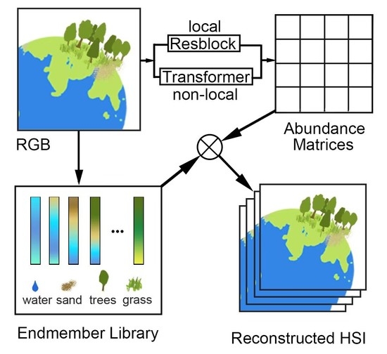
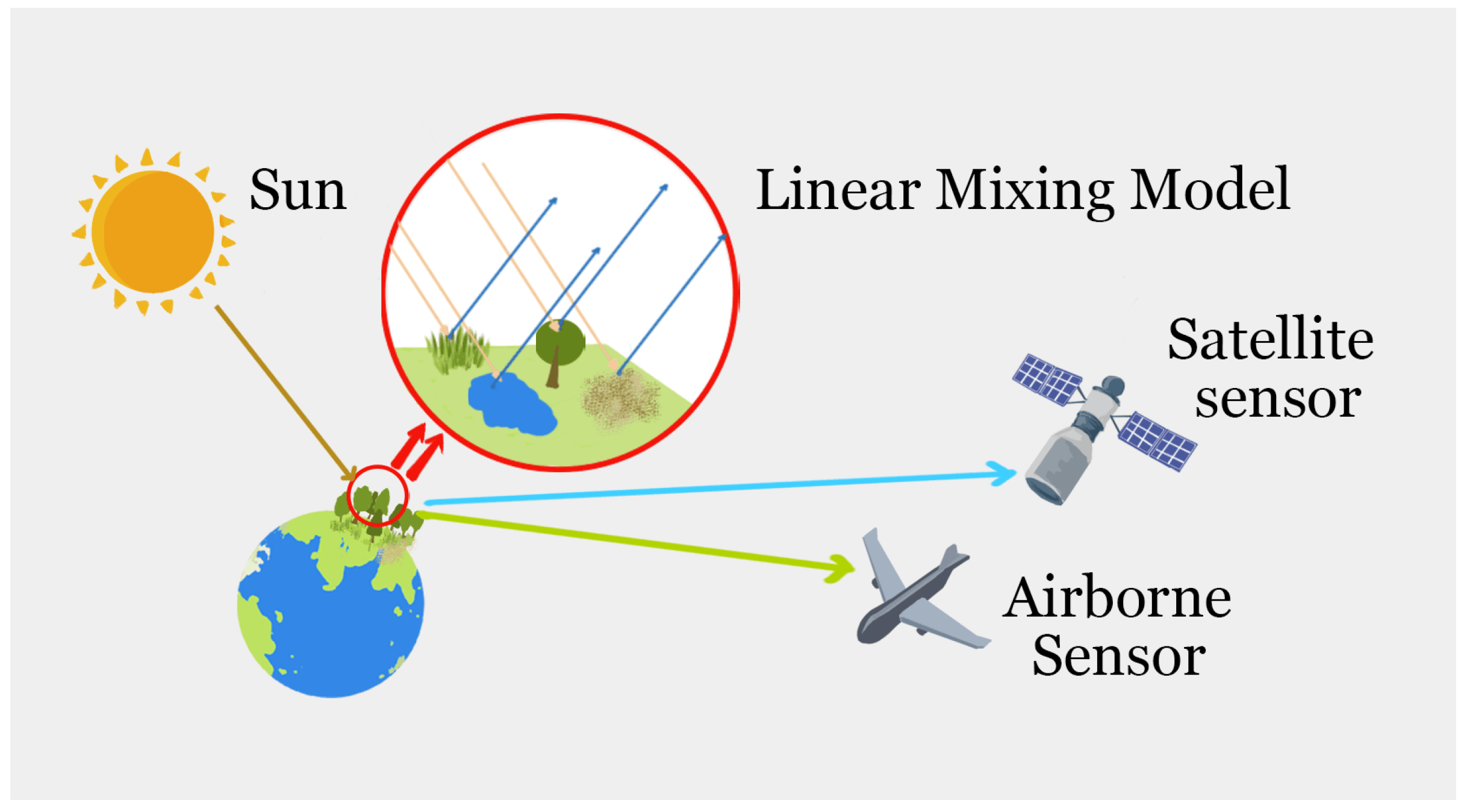
We introduce an SR network, the UGCT, which tackles HSI recovery from RGB tasks using the LMM as a foundation while employing convolutional transformer to drive fine spectral reconstruction. By employing an unmixing technique and convolutional transformer block, the reconstruction performance of mixed pixels has been notably enhanced. The experiments on two datasets demonstrate that our method’s performance is state of the art in the SR task.

2.

The Spectral–Spatial Aggregation Module (S2AM) adeptly fuses transformer-based and convolution-based features, thereby enhancing the feature merging capability within the convolutional transformer block. We embed the channel position encoding of the transformer into ResBlock to address positional inaccuracies during the generation of abundance matrices. Notably, such errors can lead to spectral response curve distortions in the reconstructed HSIs.

3.

The Paralleled-Residual Multi-Head Self-Attention (PMSA) module generates a more comprehensive spectral feature by synergistically leveraging the transformer’s exceptional complex feature extraction capabilities and the CNN’s geometric invariance. To the best of our knowledge, we are among the first to incorporate a parallel convolutional transformer block within the single-image SR.

2. Related Work

2.1. Spectral Reconstruction (SR) with Deep Learning

Deep learning technology in SR task encompasses two distinct aspects. The first involves a fusion method based on paired images, while the second entails a direct reconstruction approach that leverages a single image such as those from CASSI or RGB systems. In the first category, a simultaneous capture of lrHS and hrMs images is employed, both possessing the same spectral and spatial resolution as HSIs separately. For example, Yao et al. [11] views hrMS as a degenerate representation of HSI in the spectral dimension and lrHS as a degenerate representation of HSI in the spatial dimension. It is suggested to use cross-attention in coupled unmixing nets based on the complementarities of the two features. Hu et al. [13], on the other hand, employed the Fusformer to obtain the implicit connection between global features and to solve the local neighborhood issue of the finite receptive field of the convolution kernel in the fusion problem using the transformer mechanism. The training process’s data load is decreased by learning the spectral and spatial properties, respectively. However, the majority of the models’ prior knowledge was created manually, which frequently results in a performance decrease when the domain is changed. Using the HSI denoising iterative spectral reconstruction approach based on deep learning, the MoG-DCN described by Dong et al. [38] has produced outstanding results in numerous datasets.

For the second category, where only single images are input, the model will learn the inverse function of the camera response function of a sensor using a single RGB image as an example. It will separate the RGB image’s hidden hyperspectral feature data from it and then combine it with the intact spatial data to reconstruct a fine HSI. Shi et al. [15], for instance, replaced leftover blocks with dense blocks to significantly deepen the network structure and achieved exceptional results in NTIRE 2018 [20]. The pixel-shuffling layer was employed by Zhao et al. [19] to achieve inter-layer interaction, and the self-attention mechanism was used to widen the perceptual field. Cai et al. [14] presented a cascade-based visual transformer model, MST++, to address the numerous issues with convolution networks in SR challenges. Its designed S-MSA and other modules further improved the ability of model to extract spatial and spectral features and achieved outstanding results in a large number of experiments.

The aforementioned analysis reveals that most previous models predominantly focused on enhancing feature extraction capabilities while neglecting the interpretability of physical modeling. This oversight often resulted in diminished performance in practical applications. In response, an SR model with robust interpretability was developed, capitalizing on the autoencoder’s prowess in feature extraction and the simplicity of LMM. By harnessing the ability of LMM to extract sub-pixel-level features, ample spatial information is concurrently gathered from RGB images. Subsequently, high-quality HSIs are restored during the reconstruction process.

2.2. Deep Learning-Based Hyperspectral Unmixing

Several deep learning models based on mathematical or physical modeling have been suggested recently and used in real-world tests with positive outcomes due to the growing demand for the interpretability of deep learning models. Among these, HU has made significant progress in tasks such as change detection (CD), SR, and other HSI processing tasks. Guo et al. [39] utilized HU to extract sub-pixel-level characteristics from HSIs to integrate the HU framework into a conventional CD task. In order to obtain the reconstructed HSI, Zou et al. [40] used the designed constraints and numerous residual blocks to obtain the endmember matrix and abundance matrix, respectively. Su et al. [41] used the paired lrHs and hrMs to learn the abundance matrix and endmember from the planned autoencoder network and then rearranged them into HSI using the fundamental LMM presumptions.

Moreover, deep learning-based techniques are frequently used to directly extract the abundance matrix or end endmembers from the HU mechanism. According to Hong et al. [42], EGU-Net can extract a pure-pixel directed abundance matrix extraction model and estimate the abundance of synchronous hyperspectral pictures by using the parameter-sharing mechanism and the two-stream autocoder framework. By utilizing the asymmetric autoencoder network and LSTM to capture spectral information, Zhao et al. [43] were able to address the issue of inadequate spectral and spatial information in the mixed model.

Based on the aforementioned research, utilizing the HU mechanism to drive the SR task evidently improves interpretability. In light of this, our method introduces a parallel feature fusion module that combines the rich geometric invariance present in the residual blocks with the global receptive field of the transformer. This approach ensures the generation of well-defined features and aligns the channel-wise information with the endmembers of the spectral library.

2.3. Convolutional Transformer Module

The transformer-based approach has achieved great success in the field of computer vision, but using it exclusively will frequently negate the benefits of the original CNN structure and add a significant amount of computing burden. Due to this, numerous studies have started fusing the two. Among these, Wu et al. [25] inserted CNN into the conventional vision transformer block, replacing linear projection and other components, and improved the accuracy of various computer vision tasks. Guo et al. [26] linked the two in succession, created the CMT model with both benefits, and created the lightweight visual model. He et al. [27] created the parallel CNN and transformer feature fusion through the developed RAM module and the dual-stream feature extraction component.

The integration of CNN and transformer is inevitable because they are the two most important technologies in the field of image processing. Many performance comparisons between the two have produced their own upsides and downsides [44,45]. Important information will inevitably be lost when using a single module alone. It is crucial to understand how to incorporate the elements that can be derived from both. In order to perform feature fusion for the parallel structure of PMSA, the channel size of the CNN that lacks modeling [37] can be well constrained utilizing the channel information in the transformer.

3. The Proposed Method

In this section, we present an overview of the LMM in the SR network, including the development of an extensive endmember library. We then introduce the UGCT framework, as illustrated in Figure 2, and describe the HSI reconstruction process, comprising the abundance generator framework and LMM architecture. Furthermore, we provide a comprehensive account of the convolutional transformer architecture, driven by the fine abundance generator, as depicted in Figure 3. Subsequently, the PMSA and S2AM are discussed, which are two crucial components of feature extraction. The process of seamlessly integrating transformer and ResBlock features within S2AM will be thoroughly illustrated in Figure 4. Lastly, we explore the loss function and delve into the implementation and configuration of various details.

3.1. Hu-Based Modeling

During the imaging process of airborne and spaceborne hyperspectral image sensors, a considerable amount of spatial information becomes intermingled within mixed pixels due to factors such as atmospheric absorption, sensor performance complexity, and the actual distribution of ground objects. This substantially reduces the spatial resolution of HSIs. At present, HU is among the most effective algorithms for addressing pixel mixing, with the LMM being one of the most well-developed fundamental modeling algorithms [46]. The HSI, $\mathit{Y}\in {\mathbb{R}}^{H\times W\times C}$, composed of mixed pixels can be divided into finite pure pixels $\mathit{r}\in {\mathbb{R}}^{N\times C}$ and corresponding abundance matrices $\mathit{A}\in {\mathbb{R}}^{H\times W\times N}$ in the classic LMM model.

$$\mathit{Y}=\mathit{A}\mathit{r}+\mathit{b}$$

(1)

in which $\mathit{b}\in {\mathbb{R}}^{H\times W\times C}$ means the noise matrices, H and W represent the spatial scale and N is the number of the endmembers.

With the help of Equation (1), we can create HSIs with high spatial resolution at sub-pixel scales by obtaining a complete endmember library $\mathbb{L}$ of HSIs and their corresponding fine abundance matrices. Because of the low spatial resolution of hyperspectral imaging, multiple ground objects are quite common in the same pixel. Within a mixed pixel, the abundance matrix describes the pure pixel content ratio. According to the basic assumption in the LMM [47], only one reflection and refraction of light occurs between emitting and being captured by the sensor.

$${\mathit{y}}_n=\sum _{i=1}^N{\alpha }_i{\mathit{r}}_i+\beta$$

(2)

where ${\alpha }_i\in \mathit{A}$ and ${\mathit{r}}_i\in \mathit{r}$ and ${\mathit{y}}_n$ represent the n-th pixel in the mixing HSI. It should be noted that ${\mathit{r}}_i$ is the i-th endmember vector from a well-known complete spectral library, which represents continuous spectral data obtained by sensors under pure light from certain pure ground objects such as bushes and gravels. Furthermore, ${\alpha }_i$ is the spectral abundance of the i-th endmember corresponding to the nth mixed pixel. The $\beta$ denotes noise disturbances, which include complex atmospheric noise as well as environmental disturbances. It is simply modeled as a bias matrix due to difficulties in accurate modeling or being eliminated in the preprocessing section.

The abundance matrix has practical physical significance, and during calculation, LMM specifies two constraints for it: a sum-to-one constraint and a non-negative abundance constraint [31]. Because the information content of the mixed pixel cannot exceed that of the pure pixel itself in the actual imaging process and because the proportion of a pure pixel included in the pixel cannot be negative, the following constraints will be used:

$${\alpha }_i\ge 0;{\mathbf{\alpha }}^{\top }\mathbf{1}=1$$

(3)

The entire spectrum library $\mathbb{L}$ is already available which was obtained in the laboratory and during onboard practical testing [48]. As a result, obtaining a fine abundance matrix from a single RGB image input is central to improving the performance of spectral reconstruction tasks based on the HU mechanism. This does not imply that we will only use the weak spectral information in RGB to reconstruct a complete HSI. On the contrary, the highly effective, complete, and pure pixels collected will be used as a key reference index to guide model training. In fact, for a high level of a priori comprehensiveness, a deep layer-by-layer autoencoder network utilizing a convolutional transformer will be used.

3.2. The Struction of UGCT

In our network, we employ the Unmixing-Guided Convolutional Transformer Abundance Generator (UGCA) in Figure 3, denoted as $\mathcal{F}$, which is specifically designed for the generation of fine abundance matrices. By providing an accurate remote sensing RGB and a complete spectral set [48] of endmembers from the relevant band, the created network will recover all of its abundance values pixel by pixel using learnable parameters ${\mathbf{\theta }}_l$ and then combine them into a complete spectral abundance matrix.

$$\begin{array}{cc}\hfill \mathit{A}=\mathit{Soft}& \hfill \left(\overline{\mathit{A}}\right)=\mathcal{F}\left(\overline{\mathit{X}}\right|{\mathbf{\theta }}_l)\hfill \end{array}$$

(4)

in which $\overline{\mathit{X}}$ represents the upsampled RGB input and $\mathit{Soft}(·)$ stands for the softmax operator in order to fit the sum-to-one constraint in Formula (3).

$$\begin{array}{c}\hfill \overline{\mathit{X}}=Upsampling\left(\mathit{X}\right)\end{array}$$

(5)

In an effort to emulate the complex mixing process of light propagation, an autoencoder approach is employed to obtain the full abundance. In this method, the input RGB $\mathit{X}$ must first undergo a predefined spectral upsampling to map it to the initial spectral features $\overline{\mathit{X}}$. As illustrated in Figure 3, the abundance matrix $\mathit{A}$ is processed through an encoding–decoding procedure where upsampling and downsampling modules are modeled as conv4 and deconv layers, respectively, to facilitate the spatial feature transformation while accommodating the corresponding channel dimension changes.

It is worth noting that this may lead to redundant features and parameters if upsampling and downsampling operations are not incorporated in an autoencoder framework [14], which inevitably leads to redundant features and parameters. To alleviate the pressure from excessive parameters and invalid repetitive features on the training process, they are widely employed in such frameworks. Specifically, as the encoder progresses deeper, the channel dimension will gradually undergo upsampling, while the spatial dimension will experience downsampling. Subsequently, in the decoder section, the spatial dimension is incrementally upsampled in accordance with the input feature scale. Concurrently, the processing of spatial dimensions facilitates the model in acquiring features at different scales. Overall, the model is designed with a symmetric architecture and employs a Conv2D (mapping) layer after the original skip connection to map the features to the desired abundance matrix.

$$\begin{array}{c}\hfill \overline{\mathit{A}}=Map({\mathit{PMSA}}^{\left(n\right)}\left(\overline{X}\right)+\overline{X}|{\theta }_{map})\end{array}$$

(6)

The input hyperspectral features undergo processing through an n-layer PMSA ${\mathit{PMSA}}^{\left(n\right)}$ module, which encodes them into abundance features using trainable parameters. A skip connection is then employed to project these features into refined abundance representations that fulfill the specified requirements. The n-layer PMSA module can be dissected into three primary components: encoder, bottleneck, and decoder.

$${\mathit{PMSA}}_{encoder}^i={[{\mathit{f}}_T^{i-1}\otimes {\mathit{f}}_C^{i-1}]}^{\downarrow }$$

(7)

During the encoder phase, the original features are partitioned into two separate streams, which are subsequently processed by transformer blocks and residual blocks (ResBlock). Distinct from conventional transformer blocks, the PMSA module harnesses the combined power of convolutional and transformer networks’ prior knowledge to execute accurate abundance extraction driven by local and non-local information.

The i-th encoder module, denoted as ${\mathit{PMSA}}_{encoder}^i$, employs a S2AM ⊗ to integrate the two acquired features, thereby maximizing their exceptional extraction capabilities in both spatial and channel dimensions. Following this, a downsampling operation ↓ is utilized to guarantee that no erroneous features impede the learning process while expanding band dimensions. Within the S2AM module in the encoder, image features undergo upsampling (doubling) in the channel dimension. To prevent the generation of an excessive number of redundant features, spatial downsampling operations ↓ prove to be highly advantageous. To avert irregularities during model training, a finer feature representation is either recommended for subsequent computation or utilized in a skip connection, ensuring a more stable and accurate learning process.

$${\mathit{PMSA}}_{decoder}^j=Concat{({\mathit{PMSA}}_{encoder}^i,{\mathit{PMSA}}_{decoder}^{j-1})}^{\uparrow }$$

(8)

The encoder process maps hyperspectral features to abundance matrix features within the bottleneck section while maintaining consistent feature spatial and spectral scales. In the subsequent decoder step, spectral features and abundance features from the prior decoder section are amalgamated in the channel dimension using the concatenation operation.

Contrasting the previously described encoder module, the decoder section ${\mathit{PMSA}}_{decoder}$ upsamples features in the spatial dimension to augment the spatial information of the abundance matrix features while simultaneously compressing channel characteristics. Spatial upsampling ↑ and channel downsampling operations are implemented within the same deconvolution layer in order to maintain the symmetry of the autoencoder structure. This method ensures an effective balance between spatial and spectral information in the final abundance matrix feature.

Finally, we will discuss in detail the issue of setting the number of blocks in the Discussion section.

3.3. Paralleled-Residual Multi-Head Self-Attention

A Paralleled-Residual Multi-Head Self-Attention (PMSA) block is composed of four key components: two parallel convolutional transformer blocks, an S2AM, and a sampling module (either upsampling or downsampling, excluding the bottleneck layer). In this architecture, the input features are explicitly divided into two separate parts, which are then fed independently into the CNN and transformer blocks.

$$\begin{array}{cc}\hfill {\widehat{\mathit{X}}}^i& \hfill =MSA\left({\mathit{X}}^{i-1}\right)+{\mathit{X}}^{i-1}\hfill \\ \hfill {\mathit{X}}_t^i& \hfill =FFN\left({\widehat{\mathit{X}}}^i\right)+{\widehat{\mathit{X}}}^i\hfill \end{array}$$

(9)

in which $MSA$ means the multi-head self-attention module, and $FFN$ consists of three Conv2D and two GELU operations.

In the ResBlock, as illustrated in Figure 4, the input must first undergo two consecutive 2D convolution and batch normalization layers (Conv2D+BN). The inclusion of a residual connection assists the model in training and converging more effectively. In the encoder and decoder part, the final ShortCut operation becomes a 2D convolution with a convolution kernel of one, while in the bottleneck section, this part is set as an empty layer.

The PMSA block leverages the strengths of both the CNN and transformer architectures to process multi-scale features effectively. The block can capture both local and global contextual information simultaneously. The parallel transformer and CNN outputs are combined in the feature fusion S2AM module to further improve the model’s capacity for pattern recognition. Finally, the sampling module adjusts the spatial resolution of the features as required, depending on the specific layer in the network.

$$\begin{array}{cc}\hfill {\mathit{X}}^i& \hfill ={[{\mathit{X}}_t^i\otimes {\mathit{X}}_c^i]}^{\downarrow }\hfill \end{array}$$

(10)

The main distinction between features ${\mathit{X}}_t^i$ and ${\mathit{X}}_c^i$ lies in their methods for handling scale within their respective blocks. Feature ${\mathit{X}}_t^i$ implements channel upsampling within the resblock, which results in an increase in the number of channels while preserving spatial dimensions. On the other hand, Feature ${\mathit{X}}_c^i$ maintains the same scale within the transformer block, retaining both the spatial dimensions and the number of channels. The S2AM is then employed to fuse the features from both ${\mathit{X}}_t^i$ and ${\mathit{X}}_c^i$, even though they have different scales. This fusion process enables the model to combine the information from various scales effectively, capturing diverse contextual information and improving the overall performance of the network.

Specifically, as depicted in Figure 2, within the encoder section, we first take input ${\mathit{X}}^{i-1}\in {\mathbb{R}}^{h,w,c}$ and feed it into the parallel convolutional transformer section. Following this, it passes through a channel upsampling module with a convolution with one kernal size in ShortCut(), and ${\mathit{X}}_c^i\in {\mathbb{R}}^{h,w,2c}$ is output after ResBlock. Subsequently, within the built-in upsampling module of S2AM, features ${\mathit{X}}_c^i$ and ${\mathit{X}}_t^i\in {\mathbb{R}}^{h,w,c}$ are fused to produce output ${\overline{\mathit{X}}}^i\in {\mathbb{R}}^{h,w,2c}$. To reduce feature redundancy and prevent additional complexity, spatial downsampling is applied to ${\overline{\mathit{X}}}^i$, ultimately yielding ${\mathit{X}}^i\in {\mathbb{R}}^{\frac{h}{2},\frac{w}{2},2c}$. In a similar manner, the decoder section will exhibit symmetry with the encoder.

3.4. Spectral–Spatial Aggregation Module

Transformer and CNN models use distinctly different priors and feature extraction techniques. We suggest the S2AM in Figure 4, which addresses ResBlock’s inaccurate assumption of channel dimensions brought on by convolutional kernel constraints [37] in order to significantly increase the benefits of both models. This module utilizes the transformer block to encode the weights of features along the channel dimension. These encoded weights are then embedded into the ResBlock to assist in aligning features along the channel dimension. This integration results in the reconstruction of a more detailed HSI.

Enhancing each feature separately and achieving feature scale alignment along the channel dimension are prerequisites for efficiently processing features ${\mathit{X}}_t^i$ and ${\mathit{X}}_c^i$ in simultaneous transmission. Both features must go through a careful preprocessing stage to achieve this.

$$\begin{array}{cc}\hfill {\widehat{\mathit{X}}}_t^i& \hfill =\mathbf{\tau }\left({\mathit{X}}_t^i\right)\hfill \\ \hfill {\widehat{\mathit{X}}}_c^i& \hfill =\mathbf{\delta }\left({\mathit{X}}_c^i\right)\hfill \end{array}$$

(11)

in which $\mathbf{\delta }$ represents a 3 × 3 dilation convolution, and $\mathbf{\tau }$ represents a group convolution. Utilizing the $\mathbf{\delta }$’s expansion factor gives features a larger spatial receptive field, which aids in capturing more contextual information from the input. Group convolution, on the other hand, helps reduce the redundant parameters introduced by the transformer during channel dimension alignment. These enhanced features can then be effectively fused and processed in subsequent layers of the network. Next, the feature ${\widehat{\mathit{X}}}_t^i$ will be encoded as a one-dimensional position code along the channel dimension.

$$\begin{array}{c}\hfill {\mathit{T}}^i={\widehat{\mathit{X}}}_c^i\odot sig\left(\pounds \left(Avgpool\left({\widehat{\mathit{X}}}_t^i\right)\right)\right)\end{array}$$

(12)

where £ stands for the fully connected layer and $sig(·)$ is the sigmoid operator to map the feature with 0–1.

It becomes difficult to model the distribution of many ground objects and their relationships when pixels are mixed. This complexity significantly affects the generation of abundance matrices, which are crucial for understanding the composition of mixed pixels in remote sensing and hyperspectral imaging applications. In the position encoder component of the S2AM, three cascaded, fully connected layers £ are employed to simulate the complex relationships between ground objects.

$$\begin{array}{c}\hfill {\mathit{X}}^{i+1}={\mathit{T}}^i+{\widehat{\mathit{X}}}_t^i\end{array}$$

(13)

In conclusion, the aligned transformer features and the position-encoded embedded ResBlock information are carefully combined through element-wise addition. This process achieves information aggregation for the transformer, enabling the model to effectively fuse the strengths of them. By integrating the position-encoded information and leveraging the S2AM module, the model is better equipped to handle the challenges of spectral reconstruction.

3.5. Loss Function and Details

Our model is specifically designed to address the single-image SR task. It begins by taking a three-channel image as input, and through model mapping, it produces a reconstructed HSI $\mathit{Y}$. To ensure that it closely resembles the ground-truth HSI $\widehat{\mathit{Y}}$, it is essential to constrain the model to learn the inverse function of the camera response function. Designing a superior loss function is a key component of achieving this objective. We primarily use the mean relative absolute error (MRAE) loss as the loss function for this purpose. By using MRAE loss, the model is encouraged to learn a more accurate mapping between the input three-channel image and the corresponding HSI, resulting in improved reconstruction quality.

$$\mathcal{L}oss(\mathit{Y},\widehat{\mathit{Y}})=\frac{1}{N}\sum _{i=1}^N\frac{|{\mathit{Y}}_i-{\widehat{\mathit{Y}}}_i|}{{\widehat{\mathit{Y}}}_i}$$

(14)

It is important to note that due to the presence of a significant number of zero values (minimum values) in some datasets (AVIRIS [49]), the MRAE loss calculation may fail. For all comparative experiments involving such datasets, we use the L1 loss as a substitute for the previously mentioned loss function.

In order to generate a more sufficient abundance matrix and subsequently reconstruct the HSI, we have adopted a dual-stream PMSA architecture to process features. This design choice enables the model to leverage the strengths of both convolutional and transformer-based methods, resulting in improved feature representation and fusion. During the design process, the number of blocks in the backbone network is set to 7, including two symmetric encoder and decoder blocks in Figure 3, with one serving as the bottleneck layer. This configuration allows for a more efficient flow of information through the network while maintaining an appropriate balance between the model’s complexity and performance.

Additionally, the spectral dimension is designed with a reference point of 32 in $\overline{\mathit{X}}$ to ensure the stability of parameter quantities and model performance. This choice helps to keep the number of model parameters at a manageable level while still achieving high-quality SR.

4. Experiments and Results

4.1. Spectral Library

The success of incorporating LMM into the SR task depends on the a priori integration of the accurate spectral library. The quality and completeness of this endmember library directly influence the model’s effectiveness in practical applications. To ensure a comprehensive and accurate data source, we have chosen the United States Geological Survey (USGS) [50] Spectral Library Version 7. This library offers an extensive collection of well-characterized reference spectra, enhancing the reliability of our model. To maximize compatibility with various hyperspectral datasets, we selected the 2014 version of the Airborne Visible/Infrared Imaging Spectrometer (AVIRIS) [49] sensor measurements, owing to its wide spectral range (0.4–2.5 $\mathsf{\mu }$m) and a fine spectral resolution of 10 nm. This choice ensures that our model can accommodate the widest possible range of hyperspectral cubes.

However, the USGS v7 includes a large number of spectra that cannot be detected by airborne or satellite-based sensors, such as those of laboratory-made substances. Including these redundant spectra not only increases the number of parameters but also potentially impacts the recontruction HSIs performance. Therefore, it is crucial to carefully curate the spectral library by eliminating irrelevant spectra and retaining only those pertinent to the specific remote sensing application.

To improve the spectral library’s precision, we first undertook a rigorous data-cleaning process. This involved the removal of officially calibrated invalid spectral locations, resulting in the elimination of 914 targets containing invalid channels. After that, we concentrated on identifying ground objects that are typically difficult to detect in remote sensing images, such as minerals and lab-created organic compounds, in their pure pixels. Through this process, we identified 1019 pure pixels that met our criteria for further analysis. In order to optimize our results, we conducted additional screening to isolate pure pixels that were not needed, as in Refs. [31,36]. This comprehensive screening process ultimately yielded 345 calibrated endmembers, which are expected to significantly improve the quality and precision of our spectral analysis.

4.2. Datasets and Training Setup

We experiment with the UGCT on the $grss\_dfc\_2018$[31] and AVIRIS [51] datasets. The IEEE $grss\_dfc\_2018$ dataset is a remote sensing dataset for change detection analysis. It was collected on 16 February 2017 by the National Center for Airborne Laser Mapping (NCALM) from Houston University. The dataset includes hyperspectral data acquired by an ITRES CASI 1500 sensor with a spectral range of 380–1050 nm and 48 bands. It covers two urban areas, Las Vegas and Paris, with a total of 180 image pairs. The original dataset consisted of 27, $512\times 512$ pixel hyperspectral image patches. We randomly selected 24 of these patches for training and 3 for testing. Since the original dataset did not provide corresponding RGB channels, we chose to superimpose the features of channels 23, 12, and 5 to create RGB input.

The AVIRIS [49] dataset is a collection of high-spectral-resolution images captured by the AVIRIS sensor, which has 224 contiguous spectral bands between 0.4 and 2.5 $\mathsf{\mu }$m and a spatial resolution of 10–20 m. Its large imaging coverage is a major advantage. After preprocessing, we extracted 48 spectral features in the 380–1050 range to form the hyperspectral image (HSI) and selected three channels similar to those in the $grss\_dfc\_2018$ dataset as RGB inputs. In total, 3768 patches of size $64\times 64$ were used as the training set, and a large image of size $500\times 1000$ was used as the validation set.

The proposed UGCT model was trained on an RTX2080Ti GPU for approximately 6 h. The training data for the model input were divided into patches of size $64\times 64$. The batch size was set to 20, and the optimizer used was Adam [52] with ${\beta }_i$ = 0.9 and ${\beta }_2$ = 0.999. The learning rate was initialized at 0.0004, and a cosine annealing [53] learning rate strategy was used for 100 epochs. Due to the limited size of the training set, random rotation and flipping augmentation methods were used to enhance the data [54].

We selected several SR methods for comparison to demonstrate the superiority of our method, including AWAN [16], HRNet [19], HSCNN+ [15], MST++ [14], and Restormer [55]. Additionally, Ours− was introduced, representing the UGCT model without LMM modeling. To ensure a fair comparison, each method was fully optimized and retrained in the same scene.

$$MRAE=\frac{1}{N}\sum _{i=1}^N\frac{|{\mathit{Y}}_i-{\widehat{\mathit{Y}}}_i|}{{\widehat{\mathit{Y}}}_i}$$

(15)

$$RMSE=\sqrt{\frac{1}{N}{\sum }_{i=1}^N{({\mathit{Y}}_i-{\widehat{\mathit{Y}}}_i)}^2}$$

(16)

To quantitatively compare the results, we used several parameters, including Root Mean Square Error (RMSE) [14,15], Mean Relative Absolute Error (MRAE), Structural SIMmilarity (SSIM) [17], Peak Signal-to-Noise Ratio (PSNR) and Spectral Angle Mapper (SAM) [56]. The RMSE, MRAE, and SAM are metrics for evaluating the accuracy of the reconstructed results, where lower values indicate better reconstruction. Meanwhile, higher SSIM and PSNR values indicate better performance.

4.3. Comparision with Other Networks

Figure 5 showcases the performance results of different methods on the $grss\_dfc\_2018$ dataset. Five channels were selected as examples to demonstrate the MRAE loss error of the comparison model on the validation set. It should be noted that if the reconstructed result performs poorly in terms of MRAE, the pixel will appear brighter. Conversely, if the reconstruction is similar to HSI, the image will appear darker as a whole.

Due to its large number of parameters, HRNet tends to overfit when faced with small sample datasets, resulting in widespread errors in the spectral response curve of a patch in Figure 6. Although HSCNN+, MST++, and Restormer generally maintain alignment in spatial features when compared to HRNet, displaying only minor and consistent distortions at the fine edges, they still exhibit more severe reconstruction errors in comparison to UGCT.

The Ours−, which removes the LMM, achieves results that are comparable to the aforementioned models. However, by incorporating spectral library priors, our method clearly provides more accurate reconstruction results. For the 830 nm feature, other approaches exhibit distortions on the streets, whereas our method, due to the inclusion of priors, demonstrates a significant advantage in maintaining the accuracy of the reconstructed HSI. Based on the data presented in

Table 1. The quantitative results of the $grss\_dfc\_2018$ validation dataset. The best and second-best methods are bolded and underlined.

Method	RMSE ↓	MRAE ↓	SSIM ↑	SAM ↓
HRNet [19]	0.2020	0.1630	0.882	8.53
AWAN [16]	0.1027	0.0757	0.970	4.64
HSCNN+ [15]	0.1001	0.0724	0.967	4.09
MST++ [14]	0.0914	0.0649	0.972	4.17
Restormer [55]	0.0973	0.0668	0.971	3.96
Ours−	0.0954	0.0614	0.977	3.89
Ours	0.0866	0.0587	0.979	3.91

, our proposed method achieves competitive results across multiple metrics. In terms of RMSE, our approach outperforms the second-best result by 0.0048, while for MRAE, our method and the UGCT variant without LMM obtain the best and second-best results, respectively. These outcomes collectively demonstrate the effectiveness of our method in comparison to the competing algorithms.

Due to the validation images in the AVIRIS dataset being large, with dimensions of $1010\times 662$, we have reduced computational costs by dividing the images into three overlapping $515\times 512$ patches. To demonstrate our results in comparison with other models, we have displayed the MRAE error maps for five selected channels in Figure 7 and the spectral response curves for two selected regions in Figure 8. The closer the curve is to the ground truth, the better the reconstruction performance, and vice versa.

As the results of

Table 2. The quantitative results of the AVIRIS validation dataset. The best and second-best methods are bolded and underlined.

Method	RMSE ↓	MRAE ↓	SSIM ↑	SAM ↓
HRNet [19]	0.1400	0.8158	0.105	59.63
AWAN [16]	0.0408	0.2141	0.779	12.30
HSCNN+ [15]	0.0775	0.4744	0.716	9.08
MST++ [14]	0.0446	0.2806	0.748	12.61
Restormer [55]	0.0324	0.1883	0.846	8.38
Ours−	0.0357	0.2424	0.875	7.71
Ours	0.0271	0.1451	0.886	6.80

demonstrate, our method achieves the best performance in all four metrics and exhibits the highest similarity to the ground truth curve in the spectral response curves. Notably, HRNet and HSCNN+ appear unable to obtain adequate training or extract sufficient features, leading to substantial distortion in the results, as depicted in Figure 7, which implies that the AVIRIS dataset, characterized by its limited data volume and elevated image noise, demands a more robust feature extraction capability from the network. In contrast, the more lightweight MST++ achieves comparatively improved results, demonstrating a markedly better fit of the spectral response curve in Figure 8 when compared to the previously mentioned methods. While the UGCT exhibits a marginally lower performance than Ours− in SAM metrics, it is evident that both methods substantially outperform other comparison techniques, which indicates the superiority of the convolutional transformer in feature extraction. It is worth noting that the removal of LMM from UGCT results in a significant decline in the performance of the three indexes, which can be attributed to the loss of prior knowledge from the spectral library. When faced with the smaller, noisier AVIRIS dataset, this approach encounters considerable challenges. However, it still manages to produce satisfactory reconstruction results, ranking near the top overall.

The superior performance of our method on the two small-sample remote sensing datasets demonstrates its enhanced reconstruction capabilities for scenes with low spatial resolution, limited sample size, and high noise when compared to alternative approaches. This improvement stems from the integration of the exceptional feature extraction capabilities in the convolutional transformer with the sub-pixel information interpretation offered by the LMM. This combination enables a more effective extraction of mixed pixel information and refined HSI reconstruction.

Specifically, we showcase the superiority of our method on the dataset through Table 1 and Table 2. Moreover, to observe the reconstruction ability of our method on remote sensing datasets from the channel dimension, we randomly selected five channel visualization error maps from two datasets, 380 mm, 530 mm, 680 mm, 830 mm and 980 mm in the $grss\_dfc\_2018$ dataset and 395 mm, 470 mm, 785 mm, 905 mm and 1035 mm in the AVIRIS dataset. It is evident that our method achieved better results/lower error (indicated by darker colors) in both complex scene regions and simple, consistent regions. This demonstrates that the local and non-local features extracted by the convolutional transformer are effectively utilized in the task. Furthermore, spectral response curves serve as a valuable method for visualizing reconstruction tasks. By observing the degree of curve fitting in the selected area, we can clearly see that our method has achieved the best results in multiple comparisons.

In summary, based on the comprehensive comparison results, we found that the Unmixing Guided Convolutional Transformer (UGCT) driven by the LMM model outperforms the model without the unmixing module Our-, indicating that the unmixing-driven model excels in spectral reconstruction tasks. Furthermore, employing the Spectral–Spatial Aggregation Module to combine the benefits of CNN and transformer models surpasses those models that use either convolution or transformer alone. Lastly, our initial attempt at utilizing the self-encoder structured convolutional transformer for SR tasks demonstrated a state-of-the-art performance.

5. Discussion

We further discuss and analyze the impact of the modules and hyperparameter settings on the results through ablation experiments. The ablation study was divided into two parts. The first part compared the performance of different parameter settings, including spectral dimension and block number. The second part focused on the internal modules of the UGCT model, including the LMM module and the PMSA module, etc.

5.1. Network Details

In the first part, we compared the performance of different parameter settings to determine the optimal configuration for spectral dimension and block number in the $grss\_dfc\_2018$ dataset. We modified the spectral dimension while keeping other parameters constant, and we evaluated the results by measuring the corresponding indicators. The results showed that when the initial spectral dimension of the $\widehat{\mathit{X}}$ channel was set to 32, the model achieved higher performance, as shown in

Table 3. Ablation study about the setting of spectral dim and block number.

Spectral Dim	RMSE	MRAE	SSIM	PNSR
8	0.0924	0.0624	0.976	25.39
16	0.0943	0.0667	0.973	25.34
32	0.0865	0.0587	0.979	25.69
48	0.0877	0.0602	0.978	25.60
Block Number	Params	RMSE	MRAE	SSIM
5	2.41M	0.0882	0.0618	0.977
7	9.56M	0.0865	0.0587	0.979
9	38.12M	0.0975	0.0678	0.969

.

In summary, for the hyperparameter design of the model, setting the spectral dimension to 32 and the block number to 7 is the optimal choice. All subsequent experiments will be conducted under these settings.

On the other hand, we also examined the effect of block number on the performance of the model while keeping the spectral dimension at 32. It should be noted that the block number significantly affects the model’s parameter count due to channel expansion, so we only conducted experiments on three block number values: 5, 7, and 9. According to the table above, although the optimal value 7 has a larger parameter compared to 5, this is a trade-off. As the block number further increases, the parameter count will sharply increase, and the performance may decrease. Therefore, 7 is a relatively better choice.

5.2. Module Ablation Analysis

In this section, we will investigate three aspects of the model: the S2AM feature fusion component, the dual-stream parallel convolutional transformer part, and the LMM module in

Table 4. The module ablation analysis in the $grss\_dfc\_2018$ validation dataset.

Description	${\mathit{R}}_{\mathit{a}}$	${\mathit{R}}_{\mathit{b}}$	${\mathit{R}}_{\mathit{c}}$	${\mathit{R}}_{\mathit{d}}$	${\mathit{R}}_{\mathit{e}}$	Ours
LMM	✔	✔	✔	✗	✗	✔
S2AM	✗	✗	✗	✗	✔	✔
Resblock	✔	✗	✔	✔	✔	✔
Transformer	✔	✔	✗	✔	✔	✔
MRAE ↓	0.0638	0.0642	0.0712	0.0674	0.0614	0.0587

.

Firstly, in the comparison between ${\mathit{R}}_{\mathit{a}}$ and Ours, we find that the removal of the S2AM module results in a significant decrease in the reconstruction capability in terms of MRAE. This is because although the PMSA block can effectively extract two excellent features, the lack of a suitable combination method may cause the features to interfere with or mask each other. The results of ${\mathit{R}}_{\mathit{a}}$ are similar to those of ${\mathit{R}}_{\mathit{b}}$, which also demonstrates the masking effect of the transformer on the ResBlock features.

Secondly, in ${\mathit{R}}_{\mathit{b}}$ and ${\mathit{R}}_{\mathit{c}}$, we tested the reconstruction effects of retaining only one part of the dual-stream model to demonstrate its working principle. Both experiments showed a decline in performance, but it is evident that the transformer plays a leading role in feature extraction, while ResBlock also has a crucial function when the S2AM module is present.

Lastly, in ${\mathit{R}}_{\mathit{e}}$, we demonstrated the crucial role of the LMM mechanism, as the loss of the excellent prior knowledge from the spectral library led to a significant decline in the results. To illustrate the impact of the implicit relationship between the spectral position encoding embedded in the S2AM module and the endmember positions in the spectral library on reconstruction accuracy, we compared Experiment ${\mathit{R}}_{\mathit{d}}$ with Experiment ${\mathit{R}}_{\mathit{e}}$. The results highlight the importance of the position encoder in S2AM.

6. Conclusions

In this study, we present a novel SR network, UGCT, which is based on the LMM. Specifically, the backbone of the UGCT model consists of several dual-stream PMSA blocks, divided into encoder, bottleneck, and decoder sections. The convolutional transformer block PMSA is a combination of the transformer model and the CNN with various levels. Additionally, considering that CNN does not explicitly model the band dimension, we propose S2AM to fuse the dual-stream features and obtain globally refined image features. To enhance the model’s interpretability and incorporate the clear prior knowledge from the spectral library, we propose an HU-based model framework. Finally, comparative experiments conducted on two small and noisy datasets demonstrate the superiority of UGCT in reconstruction accuracy and spectral response curve fitting.

References

1. Li, Y.; Shi, Y.; Wang, K.; Xi, B.; Li, J.; Gamba, P. Target detection with unconstrained linear mixture model and hierarchical denoising autoencoder in hyperspectral imagery. IEEE Trans. Image Process. 2022, 31, 1418–1432. [Google Scholar] [CrossRef] [PubMed]
2. Chhapariya, K.; Buddhiraju, K.M.; Kumar, A. CNN-Based Salient Object Detection on Hyperspectral Images Using Extended Morphology. IEEE Geosci. Remote Sens. Lett. 2022, 19, 6015705. [Google Scholar] [CrossRef]
3. Liu, H.; Yu, T.; Hu, B.; Hou, X.; Zhang, Z.; Liu, X.; Liu, J.; Wang, X.; Zhong, J.; Tan, Z.; et al. Uav-borne hyperspectral imaging remote sensing system based on acousto-optic tunable filter for water quality monitoring. Remote Sens. 2021, 13, 4069. [Google Scholar] [CrossRef]
4. Niroumand-Jadidi, M.; Bovolo, F.; Bruzzone, L. Water quality retrieval from PRISMA hyperspectral images: First experience in a turbid lake and comparison with sentinel-2. Remote Sens. 2020, 12, 3984. [Google Scholar] [CrossRef]
5. Niu, C.; Tan, K.; Jia, X.; Wang, X. Deep learning based regression for optically inactive inland water quality parameter estimation using airborne hyperspectral imagery. Environ. Pollut. 2021, 286, 117534. [Google Scholar] [CrossRef] [PubMed]
6. Li, K.Y.; Sampaio de Lima, R.; Burnside, N.G.; Vahtmäe, E.; Kutser, T.; Sepp, K.; Cabral Pinheiro, V.H.; Yang, M.D.; Vain, A.; Sepp, K. Toward automated machine learning-based hyperspectral image analysis in crop yield and biomass estimation. Remote Sens. 2022, 14, 1114. [Google Scholar] [CrossRef]
7. Arias, F.; Zambrano, M.; Broce, K.; Medina, C.; Pacheco, H.; Nunez, Y. Hyperspectral imaging for rice cultivation: Applications, methods and challenges. AIMS Agric. Food 2021, 6, 273–307. [Google Scholar] [CrossRef]
8. Khan, A.; Vibhute, A.D.; Mali, S.; Patil, C. A systematic review on hyperspectral imaging technology with a machine and deep learning methodology for agricultural applications. Ecol. Inform. 2022, 69, 101678. [Google Scholar] [CrossRef]
9. Chakraborty, R.; Kereszturi, G.; Pullanagari, R.; Durance, P.; Ashraf, S.; Anderson, C. Mineral prospecting from biogeochemical and geological information using hyperspectral remote sensing-Feasibility and challenges. J. Geochem. Explor. 2022, 232, 106900. [Google Scholar] [CrossRef]
10. Pan, Z.; Liu, J.; Ma, L.; Chen, F.; Zhu, G.; Qin, F.; Zhang, H.; Huang, J.; Li, Y.; Wang, J. Research on hyperspectral identification of altered minerals in Yemaquan West Gold Field, Xinjiang. Sustainability 2019, 11, 428. [Google Scholar] [CrossRef]
11. Yao, J.; Hong, D.; Chanussot, J.; Meng, D.; Zhu, X.; Xu, Z. Cross-attention in coupled unmixing nets for unsupervised hyperspectral super-resolution. In Proceedings of the Computer Vision—ECCV 2020: 16th European Conference (Part XXIX 16), Glasgow, UK, 23–28 August 2020; pp. 208–224. [Google Scholar]
12. Hu, J.F.; Huang, T.Z.; Deng, L.J.; Jiang, T.X.; Vivone, G.; Chanussot, J. Hyperspectral image super-resolution via deep spatiospectral attention convolutional neural networks. IEEE Trans. Neural Netw. Learn. Syst. 2021, 33, 7251–7265. [Google Scholar] [CrossRef] [PubMed]
13. Hu, J.F.; Huang, T.Z.; Deng, L.J.; Dou, H.X.; Hong, D.; Vivone, G. Fusformer: A transformer-based fusion network for hyperspectral image super-resolution. IEEE Geosci. Remote Sens. Lett. 2022, 19, 6012305. [Google Scholar] [CrossRef]
14. Cai, Y.; Lin, J.; Lin, Z.; Wang, H.; Zhang, Y.; Pfister, H.; Timofte, R.; Van Gool, L. Mst++: Multi-stage spectral-wise transformer for efficient spectral reconstruction. In Proceedings of the IEEE/CVF Conference on Computer Vision and Pattern Recognition, New Orleans, LA, USA, 19–20 June 2022; pp. 745–755. [Google Scholar]
15. Shi, Z.; Chen, C.; Xiong, Z.; Liu, D.; Wu, F. Hscnn+: Advanced cnn-based hyperspectral recovery from rgb images. In Proceedings of the IEEE Conference on Computer Vision and Pattern Recognition Workshops, Salt Lake City, UT, USA, 18–22 June 2018; pp. 939–947. [Google Scholar]
16. Li, J.; Wu, C.; Song, R.; Li, Y.; Liu, F. Adaptive weighted attention network with camera spectral sensitivity prior for spectral reconstruction from RGB images. In Proceedings of the IEEE/CVF Conference on Computer Vision and Pattern Recognition Workshops, Seattle, WA, USA, 14–19 June 2020; pp. 462–463. [Google Scholar]
17. Hu, X.; Cai, Y.; Lin, J.; Wang, H.; Yuan, X.; Zhang, Y.; Timofte, R.; Van Gool, L. Hdnet: High-resolution dual-domain learning for spectral compressive imaging. In Proceedings of the IEEE/CVF Conference on Computer Vision and Pattern Recognition, New Orleans, LA, USA, 18–24 June 2022; pp. 17542–17551. [Google Scholar]
18. Koundinya, S.; Sharma, H.; Sharma, M.; Upadhyay, A.; Manekar, R.; Mukhopadhyay, R.; Karmakar, A.; Chaudhury, S. 2D-3D CNN based architectures for spectral reconstruction from RGB images. In Proceedings of the IEEE Conference on Computer Vision and Pattern Recognition Workshops, Salt Lake City, UT, USA, 18–22 June 2018; pp. 844–851. [Google Scholar]
19. Zhao, Y.; Po, L.M.; Yan, Q.; Liu, W.; Lin, T. Hierarchical regression network for spectral reconstruction from RGB images. In Proceedings of the IEEE/CVF Conference on Computer Vision and Pattern Recognition Workshops, Seattle, WA, USA, 14–19 June 2020; pp. 422–423. [Google Scholar]
20. Arad, B.; Ben-Shahar, O.; Timofte, R.N.; Van Gool, L.; Zhang, L.; Yang, M.N. Challenge on spectral reconstruction from RGB images. In Proceedings of the Conference on Computer Vision and Pattern Recognition Workshops, Salt Lake City, UT, USA, 18–23 June 2018; pp. 18–22. [Google Scholar]
21. Arad, B.; Timofte, R.; Ben-Shahar, O.; Lin, Y.T.; Finlayson, G.D. Ntire 2020 challenge on spectral reconstruction from an rgb image. In Proceedings of the IEEE/CVF Conference on Computer Vision and Pattern Recognition Workshops, Seattle, WA, USA, 14–19 June 2020; pp. 446–447. [Google Scholar]
22. Arad, B.; Ben-Shahar, O. Sparse recovery of hyperspectral signal from natural RGB images. In Proceedings of the Computer Vision—ECCV 2016: 14th European Conference (Part VII 14), Amsterdam, The Netherlands, 11–14 October 2016; pp. 19–34. [Google Scholar]
23. He, J.; Yuan, Q.; Li, J.; Xiao, Y.; Liu, X.; Zou, Y. DsTer: A dense spectral transformer for remote sensing spectral super-resolution. Int. J. Appl. Earth Obs. Geoinf. 2022, 109, 102773. [Google Scholar] [CrossRef]
24. Yuan, D.; Wu, L.; Jiang, H.; Zhang, B.; Li, J. LSTNet: A Reference-Based Learning Spectral Transformer Network for Spectral Super-Resolution. Sensors 2022, 22, 1978. [Google Scholar] [CrossRef]
25. Wu, H.; Xiao, B.; Codella, N.; Liu, M.; Dai, X.; Yuan, L.; Zhang, L. Cvt: Introducing convolutions to vision transformers. In Proceedings of the IEEE/CVF International Conference on Computer Vision, Montreal, QC, Canada, 10–17 October 2021; pp. 22–31. [Google Scholar]
26. Guo, J.; Han, K.; Wu, H.; Tang, Y.; Chen, X.; Wang, Y.; Xu, C. Cmt: Convolutional neural networks meet vision transformers. In Proceedings of the IEEE/CVF Conference on Computer Vision and Pattern Recognition, New Orleans, LA, USA, 18–24 June 2022; pp. 12175–12185. [Google Scholar]
27. He, X.; Zhou, Y.; Zhao, J.; Zhang, D.; Yao, R.; Xue, Y. Swin transformer embedding UNet for remote sensing image semantic segmentation. IEEE Trans. Geosci. Remote Sens. 2022, 60, 4408715. [Google Scholar] [CrossRef]
28. Liu, Z.; Luo, S.; Li, W.; Lu, J.; Wu, Y.; Sun, S.; Li, C.; Yang, L. Convtransformer: A convolutional transformer network for video frame synthesis. arXiv 2020, arXiv:2011.10185. [Google Scholar]
29. He, J.; Yuan, Q.; Li, J.; Zhang, L. PoNet: A universal physical optimization-based spectral super-resolution network for arbitrary multispectral images. Inf. Fusion 2022, 80, 205–225. [Google Scholar] [CrossRef]
30. Xu, Y.; Du, B.; Zhang, L.; Cerra, D.; Pato, M.; Carmona, E.; Prasad, S.; Yokoya, N.; Hänsch, R.; Le Saux, B. Advanced multi-sensor optical remote sensing for urban land use and land cover classification: Outcome of the 2018 IEEE GRSS data fusion contest. IEEE J. Sel. Top. Appl. Earth Obs. Remote Sens. 2019, 12, 1709–1724. [Google Scholar] [CrossRef]
31. Liu, L.; Li, W.; Shi, Z.; Zou, Z. Physics-informed hyperspectral remote sensing image synthesis with deep conditional generative adversarial networks. IEEE Trans. Geosci. Remote Sens. 2022, 60, 5528215. [Google Scholar] [CrossRef]
32. Mishra, K.; Garg, R.D. Single-Frame Super-Resolution of Real-World Spaceborne Hyperspectral Data. In Proceedings of the 2022 12th Workshop on Hyperspectral Imaging and Signal Processing: Evolution in Remote Sensing (WHISPERS), Rome, Italy, 13–16 September 2022; pp. 1–5. [Google Scholar]
33. West, B.T.; Welch, K.B.; Galecki, A.T. Linear Mixed Models: A Practical Guide Using Statistical Software; CRC Press: Boca Raton, FL, USA, 2022. [Google Scholar]
34. Luo, W.; Gao, L.; Zhang, R.; Marinoni, A.; Zhang, B. Bilinear normal mixing model for spectral unmixing. IET Image Process. 2019, 13, 344–354. [Google Scholar] [CrossRef]
35. Wang, M.; Zhao, M.; Chen, J.; Rahardja, S. Nonlinear unmixing of hyperspectral data via deep autoencoder networks. IEEE Geosci. Remote Sens. Lett. 2019, 16, 1467–1471. [Google Scholar] [CrossRef]
36. Liu, L.; Zou, Z.; Shi, Z. Hyperspectral Remote Sensing Image Synthesis based on Implicit Neural Spectral Mixing Models. IEEE Trans. Geosci. Remote Sens. 2022, 61, 5500514. [Google Scholar] [CrossRef]
37. Hu, J.; Shen, L.; Sun, G. Squeeze-and-excitation networks. In Proceedings of the IEEE Conference on Computer Vision and Pattern Recognition, Washington, DC, USA, 18–23 June 2018; pp. 7132–7141. [Google Scholar]
38. Dong, W.; Zhou, C.; Wu, F.; Wu, J.; Shi, G.; Li, X. Model-guided deep hyperspectral image super-resolution. IEEE Trans. Image Process. 2021, 30, 5754–5768. [Google Scholar] [CrossRef]
39. Guo, Q.; Zhang, J.; Zhong, C.; Zhang, Y. Change detection for hyperspectral images via convolutional sparse analysis and temporal spectral unmixing. IEEE J. Sel. Top. Appl. Earth Obs. Remote Sens. 2021, 14, 4417–4426. [Google Scholar] [CrossRef]
40. Zou, C.; Huang, X. Hyperspectral image super-resolution combining with deep learning and spectral unmixing. Signal Process. Image Commun. 2020, 84, 115833. [Google Scholar] [CrossRef]
41. Su, L.; Sui, Y.; Yuan, Y. An Unmixing-Based Multi-Attention GAN for Unsupervised Hyperspectral and Multispectral Image Fusion. Remote Sens. 2023, 15, 936. [Google Scholar] [CrossRef]
42. Hong, D.; Gao, L.; Yao, J.; Yokoya, N.; Chanussot, J.; Heiden, U.; Zhang, B. Endmember-guided unmixing network (EGU-Net): A general deep learning framework for self-supervised hyperspectral unmixing. IEEE Trans. Neural Netw. Learn. Syst. 2021, 33, 6518–6531. [Google Scholar] [CrossRef]
43. Zhao, M.; Yan, L.; Chen, J. LSTM-DNN based autoencoder network for nonlinear hyperspectral image unmixing. IEEE J. Sel. Top. Signal Process. 2021, 15, 295–309. [Google Scholar] [CrossRef]
44. Zhou, H.Y.; Lu, C.; Yang, S.; Yu, Y. ConvNets vs. Transformers: Whose visual representations are more transferable? In Proceedings of the IEEE/CVF International Conference on Computer Vision, Montreal, BC, Canada, 11–17 October 2021; pp. 2230–2238. [Google Scholar]
45. Heo, B.; Yun, S.; Han, D.; Chun, S.; Choe, J.; Oh, S.J. Rethinking spatial dimensions of vision transformers. In Proceedings of the IEEE/CVF International Conference on Computer Vision, Montreal, QC, Canada, 10–17 October 2021; pp. 11936–11945. [Google Scholar]
46. Manolakis, D.; Siracusa, C.; Shaw, G. Hyperspectral subpixel target detection using the linear mixing model. IEEE Trans. Geosci. Remote Sens. 2001, 39, 1392–1409. [Google Scholar] [CrossRef]
47. Xu, X.; Shi, Z.; Pan, B. 0-based sparse hyperspectral unmixing using spectral information and a multi-objectives formulation. ISPRS J. Photogramm. Remote Sens. 2018, 141, 46–58. [Google Scholar] [CrossRef]
48. Clark, R.N.; Swayze, G.A.; Wise, R.A.; Livo, K.E.; Hoefen, T.M.; Kokaly, R.F.; Sutley, S.J. USGS Digital Spectral Library Splib06a; Technical Report; US Geological Survey: Reston, VA, USA, 2007.
49. Green, R.O.; Eastwood, M.L.; Sarture, C.M.; Chrien, T.G.; Aronsson, M.; Chippendale, B.J.; Faust, J.A.; Pavri, B.E.; Chovit, C.J.; Solis, M.; et al. Imaging spectroscopy and the airborne visible/infrared imaging spectrometer (AVIRIS). Remote Sens. Environ. 1998, 65, 227–248. [Google Scholar] [CrossRef]
50. Kokaly, R.; Clark, R.; Swayze, G.; Livo, K.; Hoefen, T.; Pearson, N.; Wise, R.; Benzel, W.; Lowers, H.; Driscoll, R.; et al. Usgs Spectral Library Version 7 Data: Us Geological Survey Data Release; United States Geological Survey (USGS): Reston, VA, USA, 2017.
51. AVIRIS Homepage. Available online: https://aviris.jpl.nasa.gov/ (accessed on 22 March 2023).
52. Kingma, D.P.; Ba, J. Adam: A method for stochastic optimization. arXiv 2014, arXiv:1412.6980. [Google Scholar]
53. Loshchilov, I.; Hutter, F. Decoupled weight decay regularization. arXiv 2017, arXiv:1711.05101. [Google Scholar]
54. Cai, Y.; Lin, J.; Hu, X.; Wang, H.; Yuan, X.; Zhang, Y.; Timofte, R.; Van Gool, L. Mask-guided spectral-wise transformer for efficient hyperspectral image reconstruction. In Proceedings of the IEEE/CVF Conference on Computer Vision and Pattern Recognition, New Orleans, LA, USA, 18–24 June 2022; pp. 17502–17511. [Google Scholar]
55. Zamir, S.W.; Arora, A.; Khan, S.; Hayat, M.; Khan, F.S.; Yang, M.H. Restormer: Efficient transformer for high-resolution image restoration. In Proceedings of the IEEE/CVF Conference on Computer Vision and Pattern Recognition, New Orleans, LA, USA, 18–24 June 2022; pp. 5728–5739. [Google Scholar]
56. Zamir, S.W.; Arora, A.; Khan, S.; Hayat, M.; Khan, F.S.; Yang, M.H.; Shao, L. Multi-stage progressive image restoration. In Proceedings of the IEEE/CVF Conference on Computer Vision and Pattern Recognition, Online, 19–25 June 2021; pp. 14821–14831. [Google Scholar]
Figure 1. Linear Mixing Model.
Remotesensing 15 02619 g001
Figure 2. The Struction of Unmixing-Guided Convolutional Transformer Network (UGCT).
Remotesensing 15 02619 g002
Figure 3. The Struction of Unmixing-Guided Convolutional Transformer Abundance Generator (UGCA).
Remotesensing 15 02619 g003
Figure 4. The Paralleled-Residual Multi-Head Self-Attention (PMSA) block and Spectral-Spatial Aggregation Module (S2AM).
Remotesensing 15 02619 g004
Figure 5. Visual error map of five selected bands on the g r s s _ d f c _ 2018 validation dataset.
Remotesensing 15 02619 g005
Figure 6. Spectral response curve of the patch (af) of the validation set for g r s s _ d f c _ 2018 .
Remotesensing 15 02619 g006
Figure 7. Visual error map of five selected bands on the AVIRIS validation dataset.
Remotesensing 15 02619 g007
Figure 8. Spectral response curve of the patch of the validation set for AVIRIS.
Remotesensing 15 02619 g008