Application of Machine Learning to Tree Species Classification Using Active and Passive Remote Sensing: A Case Study of the Duraer Forestry Zone

Abstract

The technology of remote sensing-assisted tree species classification is increasingly developing, but the rapid refinement of tree species classification on a large scale is still challenging. As one of the treasures of ecological resources in China, Arxan has 80% forest cover, and tree species classification surveys guarantee ecological environment management and sustainable development. In this study, we identified tree species in three samples within the Arxan Duraer Forestry Zone based on the spectral, textural, and topographic features of unmanned aerial vehicle (UAV) multispectral remote sensing imagery and light detection and ranging (LiDAR) point cloud data as classification variables to distinguish among birch, larch, and nonforest areas. The best extracted classification variables were combined to compare the accuracy of the random forest (RF), support vector machine (SVM), and classification and regression tree (CART) methodologies for classifying species into three sample strips in the Arxan Duraer Forestry Zone. Furthermore, the effect on the overall classification results of adding a canopy height model (CHM) was investigated based on spectral and texture feature classification combined with field measurement data to improve the accuracy. The results showed that the overall accuracy of the RF was 79%, and the kappa coefficient was 0.63. After adding the CHM extracted from the point cloud data, the overall accuracy was improved by 7%, and the kappa coefficient increased to 0.75. The overall accuracy of the CART model was 78%, and the kappa coefficient was 0.63; the overall accuracy of the SVM was 81%, and the kappa coefficient was 0.67; and the overall accuracy of the RF was 86%, and the kappa coefficient was 0.75. To verify whether the above results can be applied to a large area, Google Earth Engine was used to write code to extract the features required for classification from Sentinel-2 multispectral and radar topographic data (create equivalent conditions), and six tree species and one nonforest in the study area were classified using RF, with an overall accuracy of 0.98, and a kappa coefficient of 0.97. In this paper, we mainly integrate active and passive remote sensing data for forest surveying and add vertical data to a two-dimensional image to form a three-dimensional scene. The main goal of the research is not only to find schemes to improve the accuracy of tree species classification, but also to apply the results to large-scale areas. This is necessary to improve the time-consuming and labor-intensive traditional forest survey methods and to ensure the accuracy and reliability of survey data.

1. Introduction

Forest resources are a major component of terrestrial ecosystems and play an increasingly important role in regulating the global carbon balance and mitigating climate change [1,2,3]. The quantity and quality of forest areas are, therefore, of great importance, as is monitoring forests to ensure the stability of forest ecosystems [4]. However, traditional manual monitoring methods are not only time-consuming and labor-intensive but also subject to human error [5]. Remote sensing monitoring provides a rich source of data, and the applied remote sensing methods are constantly being updated [6]; thus, such methods have played an increasingly important operational role in the implementation of national forest inventories (NFIs).

Research using remotely sensed data to classify and map tree species dates back several decades. Several studies of tree species classification based on data sources to improve accuracy have shown that classifiers that combine image pixels with spectra outperform pure spectral classifiers [7,8,9]. Although optical remote sensing is sufficiently mature, in many cases, it is difficult to identify small differences (e.g., similar species) in land cover classification due to the similar spectral characteristics [10]. However, the accuracy of stand identification based only on single features is very limited [11]. Combining textural features and vertical structure information can improve the accuracy of the classification results obtained with optical remote sensing techniques [12]. In some research based on the optimization of classification methods, classification methods based on remotely sensed data have advantages and disadvantages; usually, different classification methods are better for different regional features [13]. The CART methodology assesses the nonparametric discriminative statistical relationships among multiple data layers and generates a binary tree [14,15]. However, the limitations of the decision tree approach are its potential for overfitting and underfitting [16]. SVMs are machine learning methods with powerful generalization capabilities [17,18]; they have been shown to be powerful for local feature recognition in images [19,20]. The RF methodology is another approach for identifying local features in images. It is an integrated learning technique that builds multiple classification trees based on random bootstrap samples of training data [21,22]. In RFs, redundant variables can be removed automatically using the best classification tree [23]. In recent years, RF has been widely used in land cover and forest classification. Ke et al. integrated spectral and LiDAR data and used machine learning decision trees to construct classification rule sets. The results of a quantitative segmentation quality assessment and the classification accuracy showed improved forest classification accuracy in image segmentation and object-based classification [24].

Drones can carry a variety of sensors that can acquire a variety of different data types and resolutions. Because UAV remote sensing data acquisition requires considerable money and has various limitations, such as flight altitude, the application of satellite active–passive remote sensing data is needed to classify the entire Duraer Forestry Zone, which contains a large range of tree species. Satellite-based studies are becoming more common due to the increasing availability of satellite data, image resolution and time series datasets, and time and computational costs [25]. Researchers reported an overall accuracy of 83.2% for a model constructed using only Sentinel-2 data and an improvement in overall accuracy (OA) for combined Sentinel-1 broadleaf and conifer groups, with significant improvements in producer accuracy (PA) and user accuracy (UA) for all species and relatively good separation of the two species, which could not be separately classified using Sentinel-1 data alone [26]. This difference was because of the time-consuming satellite data search and download activities of traditional methods and the huge storage space required for aerial remote sensing data. In addition, the increased number of classified areas and tree species affects the difficulty and workload of the classification process, requiring strong computational processing power to manage all the data and run different algorithms. Therefore, cloud-based platforms, also known as virtualized supercomputer infrastructures, provide a more user-friendly approach [27]. In this respect, Google Earth Engine (GEE) has been successful because it is a cloud-based platform used for geospatial analysis that allows users to efficiently solve the main problems related to managing large quantities of data and their storage, integration, processing, and analysis [28].

The forest resources in the Arxan region cover 80% of the area, affecting the local ecosystem and representing a national reserve forest resource and a treasure trove of ecological resources [3]. The topography of the Duraer Forestry Zone is complex and mountainous, and its slope orientation has a direct impact on the growth of forest stands. Therefore, integrating multiple data sources [29] and optimal classification features [30] and selecting the best classification method are key to the classification of tree species. The aim of this study is to provide a logical basis for forest management measures to better support the monitoring and conservation of forests and their sustainable development [31,32].

2. Materials and Methods

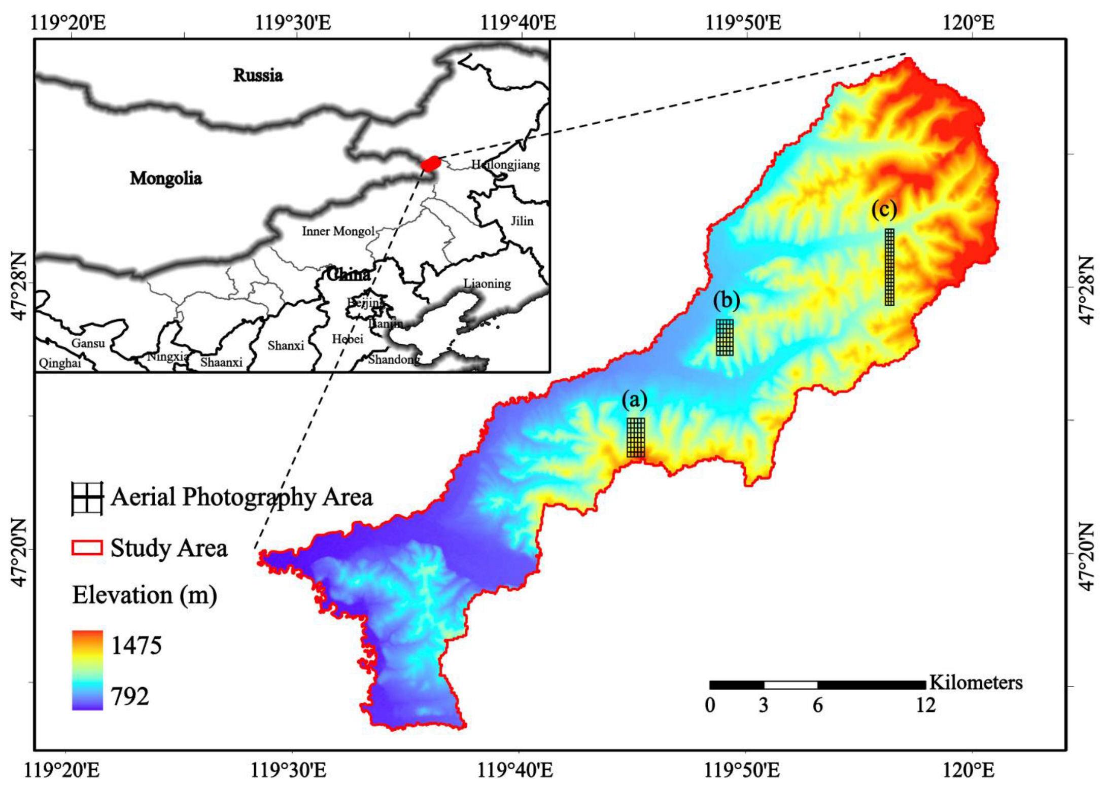
2.1. Study Area

The study area of this paper is in Duraer National Forest in Arxan, northwest of Xing’an League, Inner Mongolia Autonomous Region (119°28′–120°01′E, 47°15′–47°35′N), at the southwest foothills of the Greater Khingan Mountains, bordering Mongolia in the west and Xin Barag Right Banner in Hulun Buir, Inner Mongolia in the north (Figure 1). The total area of forestry operation is 49,812 hectares, with 33,466 hectares of forestry land, including 14,603 hectares of forested land; a total timber accumulation of 900,000 cubic meters; and a forest coverage rate of 40%. The area has a cold-temperate continental monsoon climate, with long and severe winters, hot summers with short periods of precipitation, and large daily and annual temperature differences. First, the Duraer Forestry Zone is a comprehensive management forestry plantation with natural forests (the main species is birch), planted forests (the main species is larch), farms, breeding, gathering, and wood processing. We classified three sample strips of birch and larch in the Duraer Forest with the same size from aerial photographs: sample a, 950 m × 2150 m; sample b, 910 m × 1970 m; and sample c, 450 m × 4250 m (Figure 1). The number of small classes covered by the three sample strips reached 62, with the number of forest classes being 13 and 2 major tree species being present (birch and larch). Satellite data were then used to create equivalent conditions to classify six species of trees throughout the forest site: willow, poplar, spruce, camphor pine, birch, larch, and nonforest.

2.2. Data

2.2.1. Field Survey Data

Data collected in the field included UAV multispectral data, airborne LiDAR data, UAV orthophotos, and forest sample survey data. Due to the border location of the study area, UAV flight work required multiple applications for permission. All aerial photography was completed between 10 July 2021 and 19 July 2021. Field tree survey work was performed from 10 July 2021 to 19 July 2021 and 16 to 25 July 2022. The forest survey mainly included sample coordinates, tree coordinates, community structure, woodland status, origin, slope orientation, and tree species height.

The orthophotos played an auxiliary role in building the prediction model. The main operation of the orthophoto shooting used Pegasus V10 large-load vertical takeoff and a landing unmanned aerial system (UAS) (Figure 2), and for the complex terrain of the survey area, a variable accuracy model of 8 cm for low flat areas and 13 cm for high steep standing areas was adopted for the route; the regional flight height was approximately 500 to 800 m from the ground. To ensure the accuracy of the model edge, the route exceeded the national border line by 100 to 1000 m.

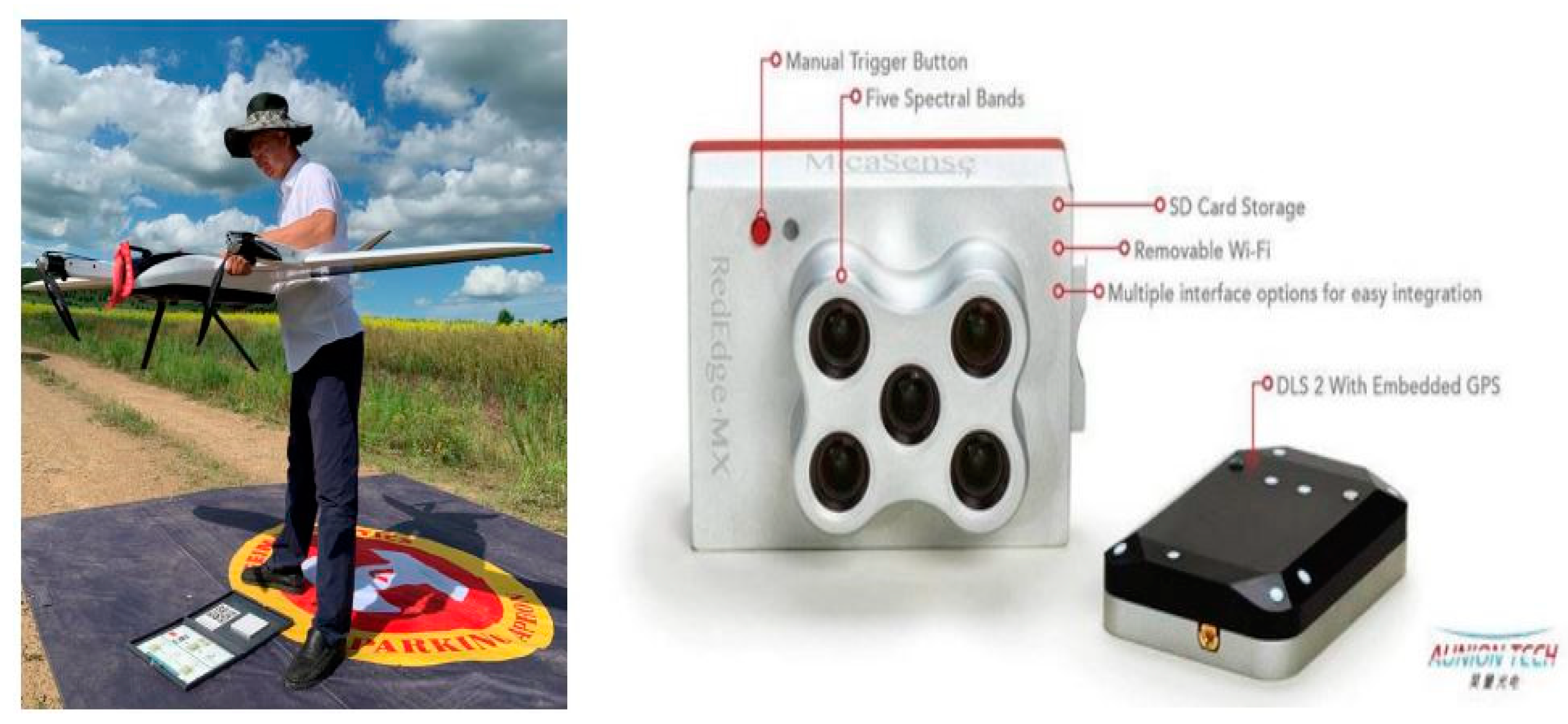
2.2.2. Drone Multispectral Data

UAV multispectral image data acquisition was performed using the Pegasus V300 product equipped with a camera model Mica Sense Red Edge-MX aerial survey (Figure 3). This product was equipped with an all-in-one multispectral imaging system, using five multispectral cameras (blue, green, red, red edge, and NIR) to form a multispectral image. There were no clouds during the aerial photography, the resolution was adjusted to 10–20 cm for the complex terrain in the survey area, the starting flight altitude was 220 m, and there was no altitude change throughout the survey; the airspeed was 16 m/s, the heading overlap was 80%, and the side overlap was 60%; the camera characteristics are shown in

Table 1. Multispectral band information.

Band	Band Name	Wavelength	Wave Width
Band 1	Blue (B)	475	20
Band 2	Green (G)	560	20
Band 3	Red (R)	668	10
Band 4	Near-infrared (NIR)	840	40
Band 5	Red edge (RE)	717	10

; and the radiation calibration was performed using a whiteboard.

The processing of the raw data was performed by the fully automated and fast UAV data processing software Pix4Dmapper from the Swiss company Pix4D. The software is based on the principle of photogrammetry and multivision reconstruction and can be used to quickly obtain point cloud data from aerial footage and process it in postprocessing. We loaded the acquired image into the software to automatically identify the coordinate information and added the image control points to obtain the stitched multispectral image.

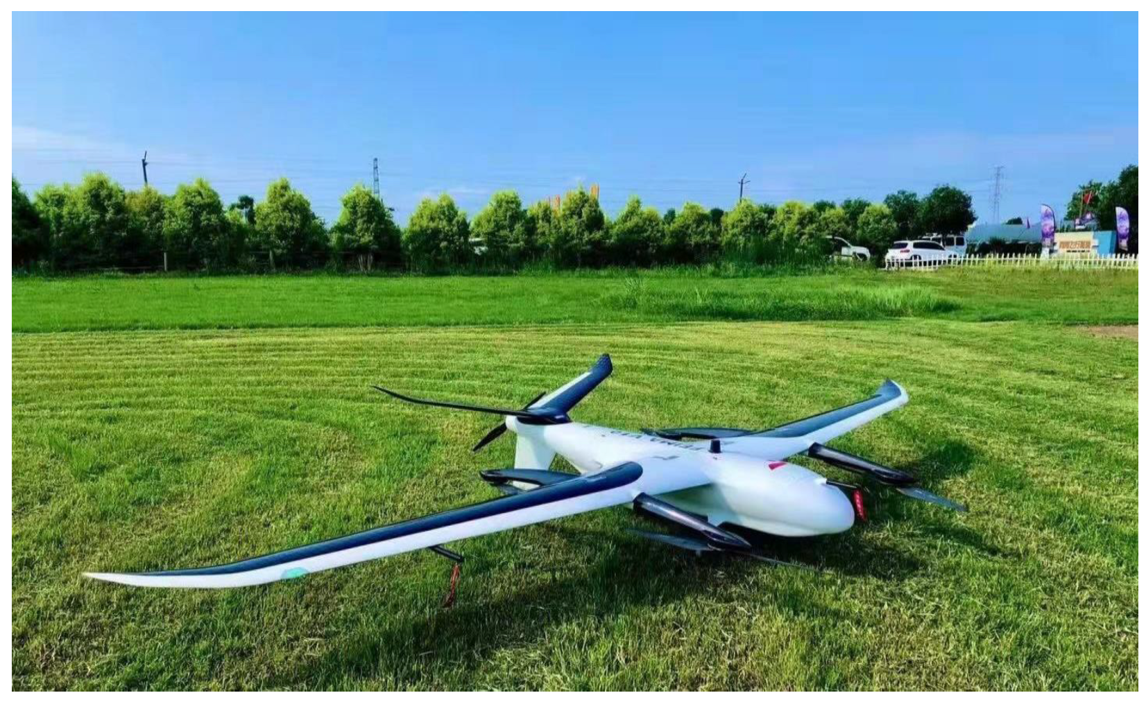
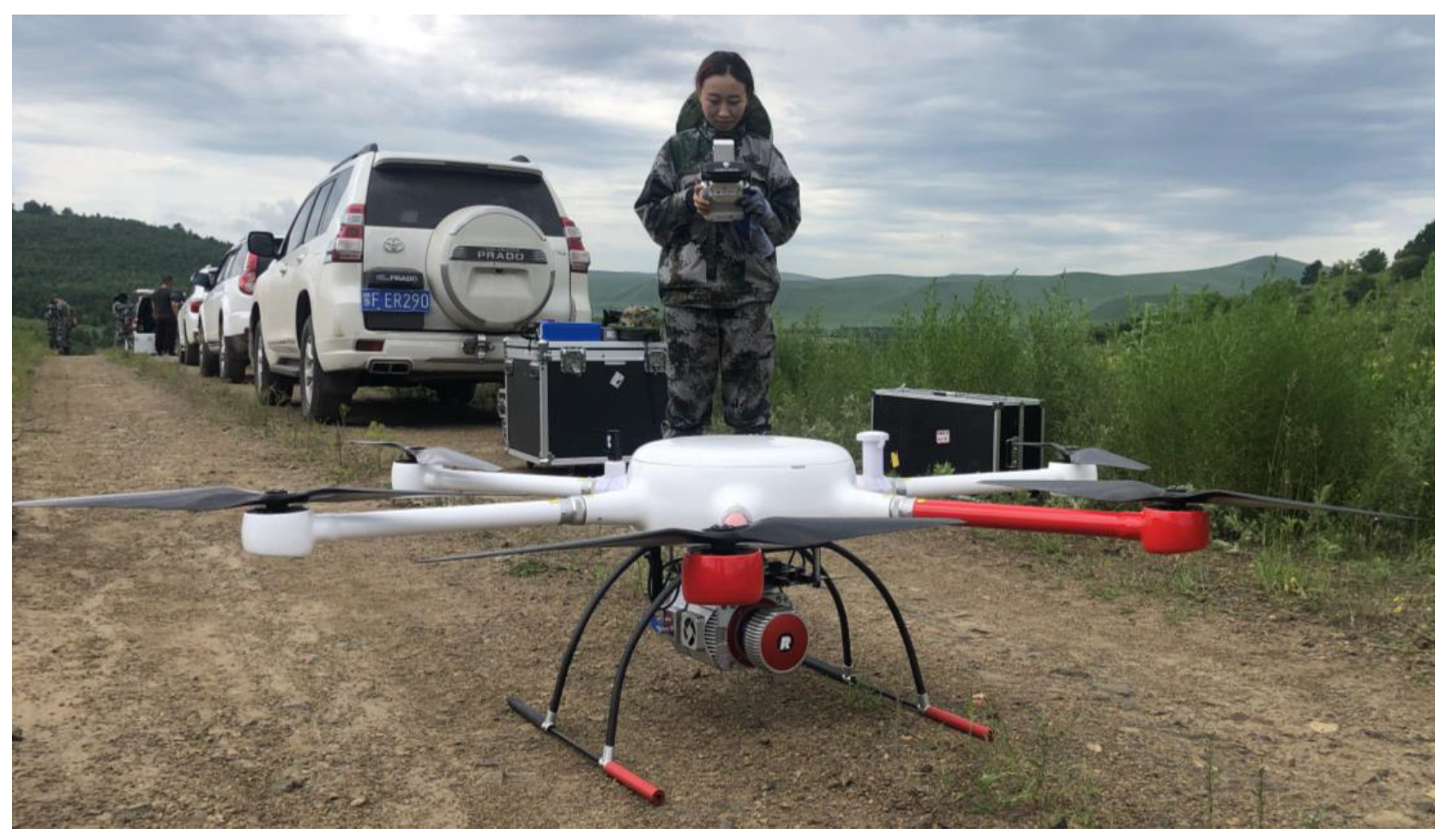
2.2.3. UAV Lidar Data

The UAV LiDAR data were collected from a Hurtigruten six-rotor UAV Long-120 equipped with the Hurtigruten ARS-1000 L long-range LiDAR measurement system (Hurtigruten, Wuhan, China) (Figure 4); the core parameters are shown in

Table 2. Lidar sensor core parameters.

Core Parameters ARS-1000 L
Maximum flight height	1350 m
Range resolution	±5 cm
Scanning angle	±330°
Angle resolution	0.001°
Pulse frequency	820 KHZ
Laser wavelength	Near-infrared
Beam divergence	0.5mrad

. LiDAR data were collected between 12 July 2021, and 17 July 2021, covering a total area of 21.8 km². The platform flew at altitudes between 200 and 400 m, with flight speeds of 6 m/s to 10 m/s and an overlap of 60% in the side direction and 70% in the heading direction. The LiDAR sensor beam divergence fraction was 0.5 rmad, so the acquired data footprint diameter was between 0.1 m and 0.2 m.

The processing of raw data was handled using Inertial Explorer (IE) postprocessing software, an open-source software developed by NovAtel’s Waypoint product group, and by UAV Butler, a one-stop commercial software for intelligent geographic information systems (GIS) launched by Pegasus Robotics. IE is powerful and highly configurable postprocessing software for processing all available GNSS IE and processing all available GNSS data for decomposition and export to the SBET (OUT) format, which is recognized by common commercial software and can provide high-precision combined navigation information, including position, velocity, and attitude information. The SBET (OUT) format is then converted to the LAS (las) format common to general geoprocessing software using the Drone Butler Smart Laser.

2.2.4. Satellite Data

The Sentinel-2 satellite carries a multispectral imager (MSI) with an altitude of 786 km; it covers 13 spectral bands with an amplitude of 290 km. The ground resolutions are 10 m, 20 m, and 60 m, and the revisit period is 10 days for one satellite and 5 days for two complementary satellites. With different spatial resolutions, from visible and near-infrared to shortwave infrared, the Sentinel-2 data are the only data with three bands in the red-edge range among the available optical data; thus, Sentinel-2 products are very effective for monitoring vegetation health information (

Table 3. Spectral bands of the Sentinel-2 sensors (S2A).

Band Number	Band Name	Band Length (nm)	Bandwidth (nm)	Resolution (m)
1	Coastal Aerosol	443.9	27	60
2	Blue	496.6	98	10
3	Green	560.0	45	10
4	Red	664.5	38	10
5	Vegetation red edge (RE)	703.9	19	20
6	Vegetation red edge (RE)	740.2	18	20
7	Vegetation red edge (RE)	782.5	28	20
8	Near-infrared (NIR)	835.1	145	10
8a	Vegetation red edge (RE)	864.8	33	20
9	Water Vapour	945.0	26	60
10	SWIR_Cirrus	1373.5	75	60
11	SWIR	1613.7	143	20
12	SWIR	2202.4	242	20

).

NASA SRTM Digital Elevation 30 m (SRTM DEM) is a joint effort between NASA and the Department of Defense’s National Mapping Agency (NIMA), as well as German and Italian space agencies, and was completed by the U.S.-launched Space Shuttle Endeavour with the SRTM system on board. The SRTM system was used to obtain a near-global DEM. This SRTM V3 product (SRTM Plus) was provided by NASA JPL and has a resolution of 1 arc second (~30 m). This dataset underwent a void-filling process using open-source data (ASTER GDEM2, GMTED2010, and NED), while other versions contained voids or were filled with voids from commercial sources.

ALOS DSM: Global 30 m v3.2 (AW3D30) is a global digital surface model (DSM) dataset with a horizontal resolution of approximately 30 m (1 arc second grid). The dataset is a DSM dataset based on the world’s 3D topographic data (5 m grid version). Version 3.2, released in January 2021, is an improved version created by reconsidering the format, ancillary data, and processing methods at high latitudes. The elevations of the AW3D DSM are calculated via an image-matching process that uses pairs of stereo-optical images. Clouds, snow, and ice are automatically identified during processing and mask information is applied.

Data processing is performed using the Google Earth Engine (GEE) code editor, an interactive environment for developing Earth Engine applications, with a central panel that provides a JavaScript code editor. The application programming interface (API) is the core functionality of GEE and is the platform that GEE users are most concerned about. Compared to the graphical user interface (GUI), the API can call all the data and functions in the GEE platform.

2.3. Methods

2.3.1. Extraction of Spectral Features and Texture Features

The vegetation index is very suitable for discriminating vegetation over large areas, where the deviation of the general reflectance curve of vegetation between red and near-infrared constitutes a variable that is sensitive to the presence of green vegetation [33]. For example, depreciation of the NDVI can distinguish unvegetated areas [34], and the EVI belongs to atmospheric impedance [35]. The RVI can assess and monitor vegetation cover [33], and the GRVI is sensitive to subtle disturbances and differences in ecosystem types due to visible red-green band reflectance [36], both of which are sensitive in densely vegetated areas. The VDVI was proposed because chlorophyll absorbs red and blue light and reflects green light, so the classification principle in the study is to determine whether the average value of red and blue light is greater than that of green light and also to distinguish between soil and plants [37]. Other vegetation indices such as the DVI and simple ratios in the NIR and blue bands are more sensitive to the spectral response of green plants [38]. The OSAVI is an optimized index of the Soil Adjusted Vegetation Index (SAVI) which can reduce soil background effects during classification [39]. The IPVI is a linear extension of the NDVI, which can avoid negative numbers during classification [40]. Details of these vegetation indices are shown in (

Table 4. Feature information in this research.

Features	Abbreviation	Formula	Reference
Normalized Difference Vegetation Index	NDVI	$\mathrm{NDVI}=\frac{\mathrm{NIR} - \mathrm{R}}{\mathrm{NIR} + \mathrm{R}}$	[34]
Ratio Vegetation Index	RVI	$\mathrm{RVI}=\frac{\mathrm{NIR}}{\mathrm{R}}$	[33]
Enhanced Vegetation Index	EVI	$\mathrm{EVI}=\frac{2.5 \ast \left(\mathrm{NIR} - \mathrm{R}\right)}{\mathrm{NIR} + 6 \ast \mathrm{R} - 7.5 \ast \mathrm{B} + 1}$	[35]
Difference Vegetation Index	DVI	$\mathrm{DVI}=\mathrm{NIR} - \mathrm{R}$	[38]
Green-Red Vegetation Index	GRVI	$\mathrm{GRVI}=\frac{\mathrm{G} - \mathrm{R}}{\mathrm{G} + \mathrm{R}}$	[36]
Infrared Percentage Vegetation Index	IPVI	$\mathrm{IPVI}=\frac{\mathrm{NIR}}{\mathrm{NIR} + \mathrm{R}}$	[40]
Near infrared and Blue Band Ratios	-	$\frac{\mathrm{NIR}}{\mathrm{B}}$	[38]
Renormalized Difference Vegetation Index	RDVI	$\mathrm{RDVI}=\frac{\mathrm{NIR} - \mathrm{R}}{\sqrt{\mathrm{NIR} + \mathrm{R}}}$	[43]
Visible-band Difference Vegetation Index	VDVI	$\mathrm{VDVI}=\frac{\left(\mathrm{G} - \mathrm{R}\right) + \left(\mathrm{G} - \mathrm{B}\right)}{\mathrm{G} + \mathrm{R} + \mathrm{G} + \mathrm{B}}$	[37]
Optimized Soil Adjusted Vegetation Index	OSAVI	$\mathrm{OSAVI}=\frac{\mathrm{NIR} - \mathrm{R}}{\mathrm{NIR} + \mathrm{R} + 0.16}$	[39]
Grayscale Symbiosis Matrix	GLCM	Mean Variance Contrast Homogeneity Dissimilarity Correlation Angular Second Moment Entropy
Edge Enhancement	-	Median Sobel Roberts User-defined
Statistical Filter	-	Data range Mean Variance Entropy Skewness

). In remote sensing, texture describes the variation between light intensity values reflected to the sensor to distinguish valuable data associated with different objects [41]. The red-edge band is valuable in measuring plant health and helping in vegetation classification [42]. The difference in reflectance between birch and larch in the images of the study area in this analysis was more obvious in the red-edge band and the near-infrared band (Figure 5), so these two bands were used in the selection of texture features. The band operation equation is given as follows.

Band = (NIR + RE)/2

(1)

* NIR: near-infrared band; RE: red-edge band

2.3.2. Extraction of Vertical Features

The digital elevation model (DEM), digital surface model (DSM), and CHM were obtained from LiDAR360 software developed by Digital Green Earth. This software can preprocess point cloud data with functions such as noise removal, ground point normalization, and extraction of various parameters.

First, the point cloud data were smoothed, resampled, and denoised to ensure that the abnormal point clouds were removed. Then, the ground points were classified, and subsequently, the DEM and DSM were extracted. After obtaining the DEM and DSM, the CHM was extracted and used to segment the airborne point cloud into single trees. Finally, the number of single tree species in a small class was estimated based on the classification results obtained. When classifying by forest landscape (coniferous, broadleaf, and mixed coniferous), we determined whether the ratio of single species in a small class reached 7:3. Simply put, if the percentage of the dominant species was 70% or less, it was considered a mixed forest. When classifying by tree species (birch, larch, mountain poplar, etc.), the specific location of each tree was verified. However, due to the limitations of airborne data, it was not possible to achieve 100% accuracy with the single-wood segmentation.

CHM = DSM − DEM

(2)

2.3.3. Classification Technique

A CART decision tree is a binary tree that can be “pruned” after it is generated [44]. That is, each nonleaf node can only lead to two branches, so when a nonleaf node is a discrete variable with multiple levels (more than 2), the variable has the potential to be used multiple times. CART can be used not only for classification but also for regression. SVMs represent a class of supervised learning that performs binary classification of data [45]. The SVM classification method separates samples belonging to different classes by tracking the maximum-edge hyperplane in the kernel space of the sample mapping [46]. An RF is an integrated classifier consisting of multiple decision trees, where the strength of individual trees and the correlation between trees can be used to generalize the error [21]. RF methodology is an augmentation of traditional decision trees that classifies new data by taking a majority vote among the classification results of all constructed decision trees [47]. In an RF, each node is split using the best combination in a randomly selected subset of feature variables at that node [31].

2.3.4. Confusion Matrix

A confusion matrix summarizes the classification results from a machine learning method in the form of a matrix that classifies the records in a dataset according to two features: the true category and the category predicted by the classification model. In this study, the results of the classification by the machine learning method were considered the predicted category, and the classification results derived from secondary forest inventory data and orthophotos were considered the true category. We analyzed the comparison matrix summarizing the number of image elements and ground tests in every category [48]. The confusion matrix can provide three descriptive accuracy metrics: overall accuracy (OA), producer accuracy (PA), and user accuracy (UA). The OA is equal to the sum of correctly classified pixels divided by the total number of pixels and directly reflects the proportion of correctly classified pixels. PA is the ratio of the number of images that the classifier correctly classifies into a category to the total number of true references in that category. UA is the ratio of the number of pixels correctly classified into a class to the total number of pixels classified into the same class by the classifier. The kappa coefficient is based on the confusion matrix and is used to assess the classification accuracy, and the higher the kappa value is, the greater the classification accuracy of remote sensing images. The value of the OA varies for each category, and the kappa value decreases once the classification result of a category is poor.

2.3.5. GEE Workflow

In the following section, we only describe the conditions created in the GEE to verify the applicability of our proposed scheme to a larger area for the equivalent of Scheme Ⅱ. Our workflow in the GEE is divided into the following main parts.

(1)

Data query and display based on the study area boundary, where the study area vector boundary (feature collection: ao) is imported and the retrieved data are cropped based on the boundary.

(2)

Extraction of the best classification elements, which include the best spectral bands, vegetation indices, and texture features (glcm), as well as the CHM derived from the DEM and DSM.

(3)

Importation of training sample data based on feature combination, for which the extracted elements are combined and imported into the region of interest (ROI).

(4)

Comparison of classification methods and accuracy check, for which the classification accuracy of three classifiers in the ROI are combined to obtain the confusion matrix. Finally, the classification results, accuracy, and kappa of each classifier are calculated, as are the PA and UA of individual tree species.

3. Results

3.1. Comparison of Tree Species Classification Schemes

When classifying image information, one should focus on how to define a meaningful set of features to describe the entire image. Once the best combination of features for classification is selected, the images can be classified using RF in machine learning methods. We designed two schemes based on the above classification features. Scheme I is a combination of the six bands of multispectral reflectance and the extracted vegetation index and texture features, while Scheme II is an additional CHM based on the combination of the six bands of multispectral reflectance and the extracted vegetation index and texture features. RF was used to assess the accuracy of the above two schemes for enhancing tree species classification. As seen in

Table 5. Comparison of the accuracy of Scheme I and Scheme II.

		Birch	Larch	Nonforest
Scheme Ⅰ	PA	80%	48%	85%
	UA	87%	51%	76%
	OA: 79%		Kappa: 0.63
Scheme Ⅱ	PA	90%	70%	84%
	UA	91%	83%	87%
	OA: 86%		Kappa: 0.75

, the overall accuracy of Scheme I was 79%, and the kappa coefficient was 0.63. The overall accuracy of Scheme II with one more CHM vertical feature was improved by 7%, and the kappa coefficient was 0.75 compared with that of Scheme I.

The results of classification Schemes I and II demonstrated that tree species classification can significantly improve the classification accuracy by increasing its vertical structure on top of the two-dimensional image. This also indicates that canopy height is effective in distinguishing forest from nonforest areas and in classifying tree species. The addition of CHM not only significantly improved the classification accuracy of birch and larch but also significantly improved the misclassification between species, and CHM had no effect on the misclassification of nonforest areas. Therefore, we believe that the hypothesis that the participation of vertical features will improve the classification accuracy of tree species is valid, i.e., Scheme II is the best classification scheme. Among the species, birch was classified most accurately by both schemes and with fewer misclassifications; larch was classified with low accuracy and with more misclassifications relative to other categories. With the addition of CHM, the classification accuracy of both birch and larch improved significantly, and the misclassification rate also decreased significantly. In particular, the classification accuracy of larch was significantly improved, and the misclassification decreased significantly; the classification accuracy of nonforest areas was also significantly improved, but the misclassification was not decreased.

As shown in (Figure 6), group (a) images show the spectral features of tree species, and group (b) includes the CHM features extracted from the point cloud data for the corresponding locations in group (a). The CHM can distinguish tree species from tree height and can compensate for misclassification caused by the shadowed part in the spectral images. Individual trees can also be classified accurately in mixed forests, and low trees do not affect the interpretation of the classifier even if they are blocked by the shadows of taller trees. Small clearings in large woods cannot be discerned spectrally, but the CHM fills this gap well. This is the advantage and notable contribution of active remote sensing in classification.

3.2. Comparison of Tree Species Classification Methods

Based on classification Scheme II, the comparison of tree classification by applying the CART, SVM, and RF is shown in Table 5. The overall accuracy of RF was higher than SVMs and the CART, with 5% and 8% improvement, respectively, and the kappa coefficient was also the highest, indicating that RF has the best classification performance. In addition, we found (

Table 6. Comparison of the classification accuracy of machine learning methods.

		RF	SVM	CART
Birch	PA	90%	93%	95%
	UA	91%	77%	75%
Larch	PA	70%	52%	44%
	UA	63%	65%	62%
Nonforest	PA	84%	72%	70%
	UA	87%	93%	90%
OA		86%	81%	78%
kappa		0.75	0.67	0.63

) that RF not only had higher classification accuracy for birch than for other categories, but also led to the lowest misclassification rate for all three categories, and the distinction between birch and larch was more accurate. Although we found that the SVMs and CART classified larch and nonforest areas slightly better than RF, they led to higher misclassification rates. Compared to the SVMs and CART, RF had the least misclassification of larch and nonforest, with 18% and 26% lower misclassification rates for larch and 12% and 14% lower misclassification rates for nonforest areas, respectively. The overall average height of birch was higher than that of the other categories, so each classification method generally classified birch higher than larch and nonforest. The overall accuracy of tree classification improved by 7% with the addition of vertical features; 4% for birch; 32% for larch; and 9% for nonforest areas; with a 10% reduction in misclassification for birch; 22% for larch; and no effect on misclassification for nonforest areas. The improvement of misclassification for larch using RF was significant compared to that for birch and nonforest areas. Overall, RF was the best tree classification method for the data source and the selected scheme of this study, as well as for the Duraer Forestry Zone site.

3.3. Spatial Distribution of the Tree Species Classification Based on RF

(Figure 7) shows the spatial distribution of tree species (birch, larch, and nonforest) areas covered by the three sample strips within the Duraer Forestry Zone in Arxan. From left to right in the figure are sample strips (a), sample strips (b), and sample strips (c). The difference image is highlighted in yellow (representing birch in the tree species classification image), orange (representing larch in the tree species classification image), and RGB (representing nonforest areas in the tree species classification image) to show the difference between the three types. The tree species classification in the figure was the result of the RF with the best accuracy. The nonforest RGB image shows that very few tree species were not classified and that small clearings in the forest were accurately classified as nonforest areas.

3.4. Spatial Distribution of the Tree Species Classification Based on GEE

Due to the different data sources, classification schemes, and classification methods used for different data products, the suitability and accuracy of data in some specific areas are often uncertain. Therefore, it is crucial to produce more precise and accurate classification products for a given region [49]. We tested the applicability of the UAV-based study protocol and the various classification features by fusing active and passive satellite data over a large study area. Regions of interest (ROIs) were established based on field-sampled data, and the accuracy of the overall classification results was assessed.

The OA of the CART decision tree classification was 0.96, and the kappa coefficient was 0.94. The OA of the SVM classifier was 0.96, and the kappa coefficient was 0.95. The results of the RF classifier with the highest accuracy are shown in (Figure 8). The OA of the RF reached 0.98, and the kappa coefficient was 0.97. The most common forest type in the Duraer Forestry Zone is natural forest (most of the coniferous forests are planted forests, which are arranged in a regular way; larch is the most planted; and spruce (landscape forest) is mostly planted along the roadside), and the UA reaches 0.98. The UA of nonforest reaches 0.99 because the addition of the CHM contributes greatly to nonforest classification. Therefore, under the same conditions the satellite data are suitable not only for large areas, but also for specific terrain areas.

(

Table 7. Confusion matrix using ground truth ROIs.

	Swamp Willow (ROI)	Poplar (ROI)	Spruce (ROI)	Sphagnum Pine (ROI)	Birch (ROI)	Larch (ROI)	Nonforest (ROI)	Total
Swamp Willow	2125	2	6	2	0	16	4	2155
Poplar	1	2259	0	1	9	23	1	2294
Spruce	7	0	2004	6	0	2	14	2033
Sphagnum pine	12	4	12	8742	16	70	7	8863
Birch	28	33	7	21	31,750	100	58	31,997
Larch	37	30	29	41	24	11,866	38	12,065
Nonforest	19	0	10	26	25	26	16,561	16,667
Total	2229	2328	2068	8839	31,824	12,103	16,683	76,074

) shows the results of the confusion matrix analysis using ground truth ROIs for the case of applying RF in GEE. To visualize the significance of the variables of the training sample and the test dataset, the rows of the matrix represent the actual categories, while the columns represent the predicted categories. Because the distribution of nonforest and birch is the widest within the Duraer Forestry Zone, the addition of CHM makes the difference in nonforest and birch height obvious. Therefore, the judgments for nonforest and birch are more accurate, and less misjudged. The confusion between birch and larch is most frequent. Most of the larch in the forest is planted, with different planting years, and some early planted larch do not differ significantly in height from immature birch, so the contribution of the CHM to the classification of these two categories is reduced. Because the differences between pine species are more obvious in the leaves, Sphagnum pine is more often misclassified as larch.

4. Discussion

Optical sensors have been widely used in classification for a long time, but they are sensitive only to the upper layers of the canopy and have low intercategory separation and high intracategory variability [50]. The quality of a sensor’s work is influenced by many environmental factors, and data need to be collected at midday when the sun is shining without cloud cover. In alpine woodland areas, the difficulty of the work can be challenging and data quality can be low due to the terrain and the forest landscape [51,52], making the data can be difficult to separate spectrally. LiDAR radar systems can identify forest canopy structures very well [53] and provide information on understory vegetation [54]. Airborne laser scanning is an active remote sensing data acquisition technique that can provide high-quality vertical structure details [55]; however, its application to forest surveys is limited by the inherent complexity of the canopy structure, and the quality of point clouds collected in naturally dense stands is usually not as good as that in sparse, evenly distributed stands [56]. In conclusion, the remote sensing data obtained from different sensors complement each other [57]. Although many data sources or region-specific methods have been proposed regarding the application of remote sensing data in tree species classification in recent decades, the application to tree species inventoried at large geographic scales remains one of the greatest challenges in this research area [58]. Z. Xie and others found that RF and SVM classification methods performed particularly well when using multisource data and that adding canopy height features to multisource data improved the classification accuracy for some tree species [39]. Researchers verified the classification of individual tree species by combining laser-scanned point clouds and spectral reflectance data and mapping the LiDAR-generated canopy features to the corresponding pixels in multispectral images, resulting in a significant improvement in the overall classification accuracy of all the classified species groups. The results of this study were also consistent with the findings of the above study, concluding that canopy height contributes to tree species classification and significantly influences the classification results among tree species.

Data redundancy may occur when machine learning methods are used to process complex categorical variables, and methods should be chosen considering whether they positively affect classification accuracy. Machine learning methods are efficient and accurate automated techniques but are prone to overfitting when processing large amounts of complex data [15,50]. RFs are integrated models with many classification trees and classifiers and work internally based on a tree pruning mechanism by automatically filtering the input classification features and then voting on the classification results to generalize the classification error [21,59]. In this study, the classification method automatically generated multiple classification trees internally. These classification trees consisted of multiple decision trees related to the reflectance of multispectral bands; the trees were used to extract multiple vegetation indices, textural signatures, and vertical structures. The design of the classification scheme was determined based on the response of the classification accuracy of the RF method to different combinations of the above indices and features. The final combination with the highest classification accuracy constituted a runnable decision tree. Until now, most of the studies on forest classification optimization based on RFs achieved greater than 90% classification accuracy. Part of the reason why the accuracy was not as high in this study was the effect of the predictive classification model when calculating the confusion matrix. The prediction model was based on the most recent forest Scheme II inventory data using the dominant tree species and established species in small classes with the aid of UAV orthophotos and field survey data. However, based on the tree species classification method, the gaps in the forest within small groups were classified as nonforest areas, and there were some large gaps or single trees in nonforest areas that differed from the predicted classification result; therefore, the classification accuracy was affected when calculating the confusion matrix. Although the classification accuracy in this paper was not as good as that of the previous classification optimization study, the objectives of this study were to investigate whether the use of the CHM could improve the classification accuracy of tree species and to compare three machine learning methods to identify the most suitable classification method for the selected study area. Therefore, the classification accuracy we observed was sufficient given the nature of the study. GEE is currently used in various fields, such as agriculture, forestry, ecology, economics, and medicine, with forest and vegetation being the most frequently applied disciplines, followed by land use and land cover [60]. Its development environment supports popular coding languages, and these core features enable users to discover, analyze, and visualize geospatial big data in a powerful way without the use of supercomputers or specialized coding knowledge [61]. In the field of remote sensing and geospatial data science, GEE has become a new method and a key tool for researchers. However, during our research, we found that the accuracy was insufficient if the training sample was too large or complex. Therefore, we relied on the training samples obtained from field surveys for accuracy testing. However, using forest type II survey data to verify accuracy may result in metrics that indicate lower modeling performance than if other less-accurate verification data are used.

In the context of ecologically sustainable development, the United Nations, to ensure the sustainable development of forest ecosystems and woodlands, established measures for different forest types to protect biodiversity and functions [62,63]. Tree species diversity is a key parameter for describing forest ecosystems [47]. The classification of tree species also plays an important role in sustainable forest management. Most of the current research on tree species classification tends to focus on how to optimize the classification results, with few targeted applications. The single-wood segmentation mentioned in this paper can extract information such as absolute coordinates, tree height, and crown width of a single wood. Combining these data with the classification results can solve the time-consuming and labor-intensive problem of traditional forest two-class inventory operations. Although airborne multispectral data and airborne LiDAR data can be effective for tree species surveys in small groups, they are also difficult to implement in forest surveys due to their relatively expensive acquisition costs. Due to the geographical environment of the Duraer Forestry Zone and the natural dense birch forest, the difficulty of airborne LiDAR scanning and data quality cannot be guaranteed. Moreover, the extraction of canopy height requires overlapping points to complement the integrity of forest canopy data, and the contribution of the CHM is affected by the small number of overlapping points in the edge of the scanned area. In addition, the larch in the study area was of an immature plantation forest, so the classification may be confused with taller shrubs (marsh willow, mountain wattle, hoodia, etc.) in terms of height, thus affecting the classification accuracy. In this regard, time series data may improve the identification of larch and thus the classification accuracy of tree species in the entire forest. Recently, some researchers have proposed alpha integrals that can integrate multi-class classifiers, which can combine the best scores to each class by all classifiers separately, thus breaking the limitations of individual classifiers and optimizing the classification results [64,65]. Therefore, the most critical factor to optimize tree species classification is to find the best classification method for individual tree species. Eventually, multiple classification models are fused to obtain the best tree species classification results.

5. Conclusions

The main findings of this paper can be summarized with the following points.

(1)

When the classification features were selected, we found that the addition of the CHM to the combination of spectral and textural features for classification improved the overall classification results, indicating that the CHM is an important indicator for improving the classification accuracy of tree species and is important in distinguishing forest from nonforest and white birch from larch.

(2)

Comparing the accuracy of machine learning methods under the conditions of choosing equal classification elements, we observed the clear advantage of the random forest among a group of machine learning methods when classifying tree species. This also indicated that RF was the best tree classification method applicable to the data source and the selected scheme of this paper and to the Duraer Forestry Zone.

(3)

Our study showed that combining the spectral features, textural features, and vertical features of multisource data (UAV multispectral, LiDAR data, and auxiliary data) and using RF could effectively improve the forest species classification accuracy in the three sample strips within the Duraer Forestry Zone in Arxan.

(4)

When applied to a large area following the above research process, the use of the GEE program combined with the required satellite data can support accurate, complex, and rapid tree species classification. The classification results are not limited to specific environments or in cases with data-limited conditions.

References

1. Dixon, R.K.K.; Solomon, A.; Brown, S.; Houghton, R.; Trexier, M.; Wisniewski, J. Carbon Pools and Flux of Global Forest Ecosystems. Science 1994, 263, 185–190. [Google Scholar] [CrossRef] [PubMed]
2. Hansen, M.C.; Potapov, P.V.; Moore, R.M.; Hancher, M.; Turubanova, S.; Tyukavina, A.; Thau, D.; Stehman, S.; Goetz, S.; Loveland, T.R.; et al. High-Resolution Global Maps of 21st-Century Forest Cover Change. Science 2013, 342, 850–853. [Google Scholar] [CrossRef] [PubMed]
3. Zhao, J.; Xie, H.; Ma, J.; Wang, K. Integrated remote sensing and model approach for impact assessment of future climate change on the carbon budget of global forest ecosystems. Glob. Planet. Change 2021, 203, 103542. [Google Scholar] [CrossRef]
4. Grabska, E.; Hostert, P.; Pflugmacher, D.; Ostapowicz, K. Forest Stand Species Mapping Using the Sentinel-2 Time Series. Remote Sens. 2019, 11, 1197. [Google Scholar] [CrossRef]
5. Bouvier, M.; Durrieu, S.; Fournier, R.; Renaud, J. Generalizing predictive models of forest inventory attributes using an area-based approach with airborne LiDAR data. Remote Sens. Environ. 2015, 156, 322–334. [Google Scholar] [CrossRef]
6. Barrett, F.; McRoberts, R.E.; Tomppo, E.; Cienciala, E.; Waser, L.T. A questionnaire-based review of the operational use of remotely sensed data by national forest inventories. Remote Sens. Environ. 2016, 174, 279–289. [Google Scholar] [CrossRef]
7. Franklin, S.E.; Peddle, D.R. Classification of SPOT HRV imagery and texture features. Int. J. Remote Sens. 1990, 11, 551–556. [Google Scholar] [CrossRef]
8. Soh, L.-K.; Tsatsoulis, C. Texture analysis of SAR sea ice imagery using gray level co-occurrence matrices. IEEE Trans. Geosci. Remote Sens. 1999, 37, 780–795. [Google Scholar] [CrossRef]
9. Zou, X.; Li, D. Application of image texture analysis to improve land cover classification. WSEAS Trans. Comput. Arch. 2009, 8, 449–458. [Google Scholar]
10. Xie, Y.; Sha, Z.; Yu, M. Remote sensing imagery in vegetation mapping: A review. J. Plant Ecol. 2008, 1, 9–23. [Google Scholar] [CrossRef]
11. Brovkina, O.V.; Cienciala, E.; Surový, P.; Janata, P. Unmanned aerial vehicles (UAV) for assessment of qualitative classification of Norway spruce in temperate forest stands. Geo-Spat. Inf. Sci. 2018, 21, 12–20. [Google Scholar] [CrossRef]
12. Deur, M.; Ga\vsparović, M.; Balenovic, I. Tree Species Classification in Mixed Deciduous Forests Using Very High Spatial Resolution Satellite Imagery and Machine Learning Methods. Remote Sens. 2020, 12, 3926. [Google Scholar] [CrossRef]
13. Chen, W.; Xie, X.; Wang, J.; Pradhan, B.; Hong, H.; Bui, D.; Duan, Z.; Ma, J. A comparative study of logistic model tree, random forest, and classification and regression tree models for spatial prediction of landslide susceptibility. Catena 2017, 151, 147–160. [Google Scholar] [CrossRef]
14. Hssina, B.; Merbouha, A.; Ezzikouri, H.; Erritali, M. A comparative study of decision tree ID3 and C4.5. Int. J. Adv. Comput. Sci. Appl. 2014, 4, 13–19. [Google Scholar] [CrossRef]
15. Loh, W.-Y. Classification and regression trees. WIREs Data Min. Knowl. Discov. 2011, 1, 14–23. [Google Scholar] [CrossRef]
16. Song, Y.; Lu, Y. Decision tree methods: Applications for classification and prediction. Shanghai Arch. Psychiatry 2015, 27, 130–135. [Google Scholar]
17. Vapnik, V.N. The Nature of Statistical Learning Theory; Springer Science & Business Media: Berlin/Heidelberg, Germany, 2000. [Google Scholar]
18. Wallraven, C.; Caputo, B.; Graf, A.B.A. Recognition with local features: The kernel recipe. In Proceedings of the Ninth IEEE International Conference on Computer Vision, Nice, France, 13–16 October 2003. [Google Scholar] [CrossRef]
19. Pontil, M.; Verri, A. Support Vector Machines for 3D Object Recognition. IEEE Trans. Pattern Anal. Mach. Intell. 1998, 20, 637–646. [Google Scholar] [CrossRef]
20. Schüldt, C.; Laptev, I.; Caputo, B. Recognizing human actions: A local SVM approach. In Proceedings of the International Conference on Pattern Recognition, Cambridge, UK, 23–26 August 2004; Volume 3, pp. 32–36. [Google Scholar]
21. Breiman, L. Random forests. Mach. Learn. 2001, 45, 5–32. [Google Scholar] [CrossRef]
22. Sonobe, R.; Tani, H.; Wang, X.; Kobayashi, N.; Shimamura, H. Random forest classification of crop type using multi-temporal TerraSAR-X dual-polarimetric data. Sens. Lett. 2014, 5, 157–164. [Google Scholar] [CrossRef]
23. Dobrinic, D.; Gašparović, M.; Medak, D. Sentinel-1 and 2 Time-Series for Vegetation Mapping Using Random Forest Classification: A Case Study of Northern Croatia. Remote Sens. 2021, 13, 2321. [Google Scholar] [CrossRef]
24. Ke, Y.; Quackenbush, L.J.; Im, J. Synergistic use of QuickBird multispectral imagery and LIDAR data for object-based forest species classification. Remote Sens. Environ. 2010, 114, 1141–1154. [Google Scholar] [CrossRef]
25. Tassi, A.; Vizzari, M. Object-Oriented LULC Classification in Google Earth Engine Combining SNIC, GLCM, and Machine Learning Algorithms. Remote Sens. 2020, 12, 3776. [Google Scholar] [CrossRef]
26. Lechner, M.; Dostálová, A.; Hollaus, M.; Atzberger, C.; Immitzer, M. Combination of Sentinel-1 and Sentinel-2 Data for Tree Species Classification in a Central European Biosphere Reserve. Remote Sens. 2022, 14, 2687. [Google Scholar] [CrossRef]
27. Praticò, S.; Solano, F.; Di Fazio, S.; Modica, G. Machine Learning Classification of Mediterranean Forest Habitats in Google Earth Engine Based on Seasonal Sentinel-2 Time-Series and Input Image Composition Optimisation. Remote Sens. 2021, 13, 586. [Google Scholar] [CrossRef]
28. Gorelick, N.; Hancher, M.; Dixon, M.; Ilyushchenko, S.; Thau, D.; Moore, R. Google Earth Engine: Planetary-scale geospatial analysis for everyone. Remote Sens. Environ. 2017, 202, 18–27. [Google Scholar] [CrossRef]
29. Holmgren, J.; Persson, Å.; Söderman, U. Species identification of individual trees by combining high resolution LiDAR data with multi—Spectral images. Int. J. Remote Sens. 2008, 29, 1537–1552. [Google Scholar] [CrossRef]
30. Eisavi, V.; Homayouni, S.; Yazdi, A.M.; Alimohammadi, A. Land cover mapping based on random forest classification of multitemporal spectral and thermal images. Environ. Monit. Assess. 2015, 187, 291. [Google Scholar] [CrossRef]
31. Dalponte, M.; Bruzzone, L.; Gianelle, D. Tree species classification in the Southern Alps based on the fusion of very high geometrical resolution multispectral/hyperspectral images and LiDAR data. Remote Sens. Environ. 2012, 123, 258–270. [Google Scholar] [CrossRef]
32. Heinzel, J.C.; Koch, B. Investigating multiple data sources for tree species classification in temperate forest and use for single tree delineation. Int. J. Appl. Earth Obs. Geoinf. 2012, 18, 101–110. [Google Scholar] [CrossRef]
33. Bannari, A.; Morin, D.; Bonn, F.J.; Huete, A.R. A review of vegetation indices. Remote Sens. Rev. 1995, 13, 95–120. [Google Scholar] [CrossRef]
34. Trier, Ø.D.; Salberg, A.-B.; Kermit, M.; Rudjord, Ø.; Gobakken, T.; Næsset, E.; Aarsten, D. Tree species classification in Norway from airborne hyperspectral and airborne laser scanning data. Eur. J. Remote Sens. 2018, 51, 336–351. [Google Scholar] [CrossRef]
35. Baugh, W.; Groeneveld, D. Broadband vegetation index performance evaluated for a low—Cover environment. Int. J. Remote Sens. 2006, 27, 4715–4730. [Google Scholar] [CrossRef]
36. Motohka, T.; Nasahara, K.N.; Oguma, H.; Tsuchida, S. Applicability of Green-Red Vegetation Index for Remote Sensing of Vegetation Phenology. Remote Sens. 2010, 2, 2369–2387. [Google Scholar] [CrossRef]
37. Louhaichi, M.; Borman, M.M.; Johnson, D.E. Spatially Located Platform and Aerial Photography for Documentation of Grazing Impacts on Wheat. Geocarto Int. 2001, 16, 65–70. [Google Scholar] [CrossRef]
38. Wang, Y.; Lu, D. Mapping Torreya grandis Spatial Distribution Using High Spatial Resolution Satellite Imagery with the Expert Rules-Based Approach. Remote Sens. 2017, 9, 564. [Google Scholar] [CrossRef]
39. Xie, Z.; Chen, Y.; Lu, D.; Li, G.; Chen, E. Classification of Land Cover, Forest, and Tree Species Classes with ZiYuan-3 Multispectral and Stereo Data. Remote Sens. 2019, 11, 164. [Google Scholar] [CrossRef]
40. Crippen, R. Calculating the vegetation index faster. Remote Sens. Environ. 1990, 34, 71–73. [Google Scholar] [CrossRef]
41. Hernandez, I.E.R.; Shi, W. A Random Forests classification method for urban land-use mapping integrating spatial metrics and texture analysis. Int. J. Remote Sens. 2018, 39, 1175–1198. [Google Scholar] [CrossRef]
42. DigitalGlobe. The Benefits of the Eight Spectral Bands of Worldview-2; DigitalGlobe: Westminster, CO, USA, 2011. [Google Scholar]
43. Feng, Y.; Lu, D.; Chen, Q.; Keller, M.; Moran, E.; dos-Santos, M.; Bolfe, É.L.; Batistella, M. Examining effective use of data sources and modeling algorithms for improving biomass estimation in a moist tropical forest of the Brazilian Amazon. Int. J. Digit. Earth 2017, 10, 996–1016. [Google Scholar] [CrossRef]
44. Lewis-Beck, M.; Bryman, A.; Futing Liao, T. CART (Classification and Regression Trees); Sage Publications, Inc.: Thousand Oaks, CA, USA, 2004. [Google Scholar]
45. Dalponte, M.; Bruzzone, L.; Vescovo, L.; Gianelle, D. The role of spectral resolution and classifier complexity in the analysis of hyperspectral images of forest areas. Remote Sens. Environ. 2009, 113, 2345–2355. [Google Scholar] [CrossRef]
46. Camps-Valls, G.; Bruzzone, L. Kernel-based methods for hyperspectral image classification. IEEE Trans. Geosci. Remote Sens. 2005, 43, 1351–1362. [Google Scholar] [CrossRef]
47. Immitzer, M.; Atzberger, C.; Koukal, T. Tree Species Classification with Random Forest Using Very High Spatial Resolution 8-Band WorldView-2 Satellite Data. Remote Sens. 2012, 4, 2661–2693. [Google Scholar] [CrossRef]
48. Niu, Z.G.; Shan, Y.X.; Gong, P. Accuracy evaluation of two global land cover data sets over wetlands of China. Int. Arch. Photogramm. Remote Sens. Spat. Inf. Sci. 2012, XXXIX-B7, 223–228. [Google Scholar] [CrossRef]
49. Yang, Y.; Yang, D.; Wang, X.; Zhang, Z.; Nawaz, Z. Testing Accuracy of Land Cover Classification Algorithms in the Qilian Mountains Based on GEE Cloud Platform. Remote Sens. 2021, 13, 5064. [Google Scholar] [CrossRef]
50. Rodriguez-Galiano, V.F.; Ghimire, B.; Rogan, J.; Chica-Olmo, M.; Rigol-Sánchez, J.P. An assessment of the effectiveness of a random forest classifier for land-cover classification. ISPRS J. Photogramm. Remote Sens. 2012, 67, 93–104. [Google Scholar] [CrossRef]
51. Guyot, G.; Guyon, D.; Riom, J. Factors affecting the spectral response of forest canopies: A review. Geocarto Int. 1989, 4, 3–18. [Google Scholar] [CrossRef]
52. Lapini, A.; Pettinato, S.; Santi, E.; Paloscia, S.; Fontanelli, G.; Garzelli, A. Comparison of Machine Learning Methods Applied to SAR Images for Forest Classification in Mediterranean Areas. Remote Sens. 2020, 12, 369. [Google Scholar] [CrossRef]
53. Bortolot, Z.J.; Wynne, R. Estimating forest biomass using small footprint LiDAR data: An individual tree-based approach that incorporates training data. ISPRS J. Photogramm. Remote Sens. 2005, 59, 342–360. [Google Scholar] [CrossRef]
54. Frazer, G.; Magnussen, S.; Wulder, M.; Niemann, K.O. Simulated impact of sample plot size and co-registration error on the accuracy and uncertainty of LiDAR-derived estimates of forest stand biomass. Remote Sens. Environ. 2011, 115, 636–649. [Google Scholar] [CrossRef]
55. Ussyshkin, V.; Theriault, L. Airborne Lidar: Advances in Discrete Return Technology for 3D Vegetation Mapping. Remote Sens. 2011, 3, 416–434. [Google Scholar] [CrossRef]
56. Li, M.; Im, J.; Quackenbush, L.J.; Liu, T. Forest Biomass and Carbon Stock Quantification Using Airborne LiDAR Data: A Case Study Over Huntington Wildlife Forest in the Adirondack Park. IEEE J. Sel. Top. Appl. Earth Obs. Remote Sens. 2014, 7, 3143–3156. [Google Scholar] [CrossRef]
57. Lu, D.; Weng, Q. A survey of image classification methods and techniques for improving classification performance. Int. J. Remote Sens. 2007, 28, 823–870. [Google Scholar] [CrossRef]
58. Fassnacht, F.E.; Latifi, H.; Stereńczak, K.; Modzelewska, A.; Lefsky, M.A.; Waser, L.T.; Straub, C.; Ghosh, A. Review of studies on tree species classification from remotely sensed data. Remote Sens. Environ. 2016, 186, 64–87. [Google Scholar] [CrossRef]
59. Puttonen, E.; Suomalainen, J.M.; Hakala, T.; Räikkönen, E.; Kaartinen, H.; Kaasalainen, S.; Litkey, P. Tree species classification from fused active hyperspectral reflectance and LIDAR measurements. For. Ecol. Manag. 2010, 260, 1843–1852. [Google Scholar] [CrossRef]
60. Tian, S.; Zhang, X.; Tian, J.; Sun, Q. Random Forest Classification of Wetland Landcovers from Multi-Sensor Data in the Arid Region of Xinjiang, China. Remote Sens. 2016, 81, 954. [Google Scholar] [CrossRef]
61. Phan, T.N.; Kuch, V.; Lehnert, L.W. Land Cover Classification using Google Earth Engine and Random Forest Classifier—The Role of Image Composition. Remote Sens. 2020, 12, 2411. [Google Scholar] [CrossRef]
62. Tamiminia, H.; Salehi, B.; Mahdianpari, M.; Quackenbush, L.; Adeli, S.; Brisco, B. Google Earth Engine for geo-big data applications: A meta-analysis and systematic review. ISPRS J. Photogramm. Remote Sens. 2020, 164, 152–170. [Google Scholar] [CrossRef]
63. Lindenmayer, D.; Margules, C.; Botkin, D. Indicators of Biodiversity for Ecologically Sustainable Forest Management. Conserv. Biol. 2000, 14, 941–950. [Google Scholar] [CrossRef]
64. McCammon, A.L.T. United Nations Conference on Environment and Development, held in Rio de Janeiro, Brazil, during 3–14 June 1992, and the ’92 Global Forum, Rio de Janeiro, Brazil, 1–14 June 1992. Environ. Conserv. 1992, 19, 372–373. [Google Scholar] [CrossRef]
65. Salazar, A.; Safont, G.; Vergara, L.; Vidal, E. Pattern recognition techniques for provenance classification of archaeological ceramics using ultrasounds. Pattern Recognit. Lett. 2020, 135, 441–450. [Google Scholar] [CrossRef]
Figure 1. Location of the Duraer Forestry Zone and spatial distribution of the aerial photography areas; (a), (b) and (c) in the figure represent different experimental sample areas acquired by aerial photography, respectively.
Remotesensing 15 02596 g001
Figure 2. Pegasus V10 large-load vertical takeoff and landing UAV.
Remotesensing 15 02596 g002
Figure 3. Pegasus V300 UAV and camera Mica Sense Red Edge-MX introduction.
Remotesensing 15 02596 g003
Figure 4. Hurtigruten six-rotor UAV Long-120 equipped with the Hurtigruten ARS-1000 L long-range LiDAR measurement system.
Remotesensing 15 02596 g004
Figure 5. Differences in reflectance of different tree species: the red line represents the spectral reflectance of white birch; the green line represents the spectral reflectance of larch.
Remotesensing 15 02596 g005
Figure 6. (a) Spectral image (RGB) difference among tree species, (b) height (CHM) difference among tree species.
Remotesensing 15 02596 g006
Figure 7. The classification results of sample strips (ac).
Remotesensing 15 02596 g007
Figure 8. The classification results for the Duraer Forestry Zone.
Remotesensing 15 02596 g008