User-Aware Evaluation for Medium-Resolution Forest-Related Datasets in China: Reliability and Spatial Consistency

Abstract

Forest cover data are fundamental to sustainable forest management and conservation. Available medium-resolution publicly shared forest-related datasets provide primary information on forest distribution. The evaluation of relevant datasets is of great importance to learn about the differences, characterize the accuracy, and provide a reference for rational use. This study presents an evaluation and analysis of the forest-related datasets in China around 2020, including TreeCover and the forest-related layer (latter referred to as the forest datasets) in WorldCover, Esri land cover, FROM-GLC10, GlobeLand30, and GLC_FCS30. These forest datasets, that are obtained by aggregating forest-related lasses based on the classification schemes, are analyzed from spatial consistency and accuracy comparison. The results illustrate that forest datasets with 10m resolution are generally more precise than those with 30m resolution in China. WorldCover shows the highest accuracy, with producer accuracy and user accuracy of 91.4% and 87.09%, respectively. These datasets exhibit high accuracy but great spatial inconsistency. The more consistent the regions are, the more accurate the accuracy is. High consistency (≥5, i.e., classified into forests by five datasets) areas account for 56.49% of areas of forest classified (AFC), while the area of low consistency (≤2) reach 25.51% of AFC. The analysis delves into the datasets, offering a reliable reference for the usage of these datasets.

1. Introduction

Forests provide clean air and water, and play an irreplaceable role in maintaining ecological balance, protecting biodiversity, and regulating climate change. Despite the importance attached to the conservation of forests by the international community, about 420 million hectares of forest area have been lost in the past 30 years. Deforestation and forest degradation continue to occur at an alarming rate, leading to a significant reduction in biodiversity. Accurately and frequently monitoring forest cover can help to recognize the status and changes of forest resources and provide essential data for sustainable forest management and utilization. Accurate forest distribution data can be obtained through forest inventories, which are usually conducted by field surveys and remote sensing and monitoring. Due to the cost and timeliness requirements, remote sensing technology has played an increasingly important role in forest inventories. Over the past decades, forest monitoring techniques have undergone significant changes, transitioning from visual discrimination [1,2] and manual outlining [3,4] to automatic identification with spectral indexes [5]. Statistical learning methods [6,7,8] and existing LULC products have played an important role in forest study. Scholars have reviewed and summarized the research progress of remote sensing techniques in the field of forest monitoring from different perspectives, including common remote sensing techniques [9], statistical methods [10], and applications of time series remote sensing images [11].

Furthermore, some freely available forest-related layers of land cover and land use (LULC) maps and forest-related thematic maps [12] contribute to the fundamental data for forest study. Forests, as an important component of the land cover, are an indispensable part of land cover and land use (LULC) classification. It is convenient to obtain forest data via global or regional LULC datasets. However, the definition of forests varies remarkably among these datasets due to their different classification schemes. Commonly, the definition of forests in these datasets is constrained by factors such as vegetation cover, tree height, area covered, and use. The availability of this data is timelier and more accessible compared to that of data from the national forest inventory. These data are more readily available and more time-efficient than national forest inventory data.

However, there are still unanswered questions that require attention. How accurate are these datasets? How are these datasets used? Therefore, it is critical to comprehensively evaluate and analyze these datasets to promote the use of these datasets. There are some works that have contributed to helping us to use these datasets. Though great effort has been made to improve the classification accuracy, that of the current 30m LULC maps is relatively unsatisfactory. By a detailed summary of 30m maps, including LULC maps and thematic maps of four different land cover types (impervious surface, forest, agricultural land, and water), Liu et al. [13] compared and analyzed these datasets with respect to statistical accuracy and spatial consistency, and found that these datasets had poor classification accuracy in the transition zone. By emphasizing that pixel-based statistical accuracy is as important as design-based inference in the task of assessing regional uncertainty in LULC datasets, Venter et al. [14] compared the accuracy of three datasets, Dynamic World, World Cover, and Esri Land Cover, on a global scale by comparing both accuracy and spatial correlation. The results show that these datasets exhibit large errors and spatial variances across regions with different biomes, continents, and human settlement types. With southwest China as the study area, Wang et al. [15] compared and analyzed the consistency of three 10m resolution land cover products and analyzed the application potential of the existing land cover products in demonstrating desertification studies indicating that the existing products could not be directly used in studies related to stone desertification areas. Ding et al. [16] evaluated the accuracy of three LULC datasets (FROM-GLC10, Esri Land Cover, and WorldCover) in Southeast Asia (SEA) using field survey data and stratified random sampling data. They found that the WorldCover dataset showed the highest overall accuracy, but FROM-GLC10 posed advantages in the classes of farmland, water, and built-up areas. Nevertheless, these efforts are either focused on assessing the overall accuracy of the product [17,18,19,20,21,22] or are class-specific [23,24,25,26]. There is a lack of evaluations on forest-related materials to better understand and use them.

This study presents a comprehensive summary and review of six forest-related datasets, including TreeCover and the forest-related layers in WorldCover, ESRI Land Cover, FROM-GLC10, GlobeLand30, and GLC_FCS30. The main points of this paper include the following aspects. (1) An introduction to forest-related datasets around 2020 is presented, and a comprehensive summary is provided in terms of an overview of technical routes and category definitions. (2) Data processing and evaluation methods are introduced, including data pre-processing, sample selection, and evaluation indicators. (3) The evaluation results are given, describing the performance of forest-related datasets in China in terms of accuracy indicators and spatial correlation. (4) The reasons for inconsistency across these datasets are analyzed, and possible improvements in future forest research are briefly prospected.

2. Dataset Description

This section includes the basic information of the medium-resolution forest related datasets around 2020, as shown in Table 1. These data include five LULC products, namely WorldCover [27], ESRI Land Cover [28], FROM-GLC10 [29], GlobeLand30 [30,31], GLC_FCS30-2020 [32], and the forest thematic dataset TreeCover [33]. Although forest-related classes (FRCs) are available in each dataset, the definitions in different datasets show some differences, as exhibited in Table 2. In addition, this paper provides a summary and review of the methods used in the related datasets. For six datasets involved, three datasets are available at 10m resolution (WorldCover, Esri Land Cover, and FROM-GLC10), and four datasets are available at 30m resolution (GLC_FCS30-2020, GlobeLand30, and TreeCover).

WorldCover: WorldCover classifies the ground cover into 11 different classes, among which the forest-related categories are Tree cover and Mangroves. With Sentinel-2 and Sentinel-1 images as the main data sources, this dataset was generated using the gradient boosting decision tree algorithm. The classification model takes 131 features extracted from different data sources as input, including 90 features extracted from Sentinel-2 data (time-series spectral features and time-series vegetation indices), 16 features extracted from Sentinel-1, two features extracted from DEM, and 23 other spatially located features. Then the well-trained model predicts the class and class probabilities of the input data. Finally, the final global land cover map is synthesized by applying different expert rules.

Esri Land Cover: This dataset consists of nine ground cover classes. The FRC is “Trees”. This dataset was created with a deep learning semantic model (U-Net) with six bands (blue, green, red, NIR, SWIR1, SWIR2) of Sentinel-2 as input. The samples used to train the deep learning model were selected by stratified random sampling. These image patches with a size of 5 km × 5 km are scattered in 14 biomes around the world. By manual annotation, 24,000 images with pixel-level labels, which are more than five billion pixels, were finally obtained.

GlobeLand30: This dataset divides the land cover into 10 classes, with forests being one of them. The GlobeLand30 includes global land cover for the years 2000, 2010 and 2020. A pixel- and object-based method with knowledge (POK) was utilized. Object-based techniques are first used to determine the spatial extent of the objects. Then a pixel-based classifier and expert knowledge are used to identify the classes to which each pixel belongs. Based on the POK classification method, a hierarchical classification strategy is adopted to identify each class according to its priority. The results are finally merged.

GLC_FCS30-2020: GLC_FCS30-2020 is a LULC product with a fine classification system. It classifies the land surface into 29 classes. The final forest dataset is obtained by aggregating the FRC according to the mapping between the fine classification system and other classification systems [32,34]. This dataset takes a locally adaptive random forest with a 5° × 5° geographic tile as the processing base unit. The global training data for model training is generated from the Landsat year-composited surface reflectance imagery and Global Spatial Temporal Spectra Library, which is developed by filtering Climate Change Initiative Global Land Cover (CCI_LC) and MODIS Nadir Bidirectional Reflectance Distribution Function-Adjusted Reflectance (MCD43A4 NBAR).

FROM-GLC10: FROM-GLC10 exhibits the global land cover in 2017 including 10 classes. The FRC of this dataset is “Forest”. This dataset was produced with a random forest classification algorithm and Sentinel-2 images. Features used for classification include spectral bands, spectral indexes (such as vegetation, water, building, and snow index), location, and terrain features (including slope and aspect). The samples used for training are collected in the previous LULC classification task. The results show that when the number of training samples reaches a certain size, stable classification can still be achieved even if there is a 20% error in the global training sample points.

TreeCover 2000 and Global Forest Change dataset: These two datasets are released by the Global Land Analysis and Discovery (GLAD) laboratory in the Department of Geographical Sciences at the University of Maryland. TreeCover 2000 represents global tree canopy cover at the peak of the 2000 growing season. Global Forest Change, which has been updated to Global Forest Change 2021 v1.9, shows global forest change after 2000. For these datasets, a bagged decision tree methodology was employed, with the Landsat time-series spectral features and vegetation index features as inputs.

Table 1. Medium resolution forest datasets around 2020.

Dataset	Period	Satellites	Resolution	Accuracy	Method
WorldCover (https://zenodo.org/record/5571936#.ZEjQ_Y9BxaR, accessed on 7 April 2023)	2020	Sentinel-2 Sentinel-1	10 m	OA: 74.4% Tree cover: PA: 89.9%, UA: 80.8% Mangroves: PA: 51.5%, UA: 68.6%	Gradient boosting decision tree (CatBoost)
Esri Land Cover (https://www.arcgis.com/apps/instant/media/index.html?appid=fc92d38533d440078f17678ebc20e8e2, accessed on 7 April 2023)	2020	Sentinel-2	10 m	OA: 85.96% Treecover: PA: 91.07%, UA: 90.35%	Deep learning (U-Net)
GlobeLand30 (http://www.globallandcover.com/home.html?type=data, accessed on 7 April 2023)	2020	Landsat HJ-1 GF-1 WFV	30 m	OA: 85.72%; Kappa: 0.82	Pixel- and object-based methods with knowledge
GLC_FCS30 (https://data.casearth.cn/sdo/detail/5fbc7904819aec1ea2dd7061, accessed on 7 April 2023)	2020	Landsat	30 m	OA: 82.5%; Kappa:0.78 [35]	A local adaptive random forest
FROM-GLC10 (http://data.ess.tsinghua.edu.cn/fromglc2017v1.html, accessed on 7 April 2023)	2017	Sentinel-2	10 m	OA: 72.76% Forest: PA: 84.20%, UA: 83.47%	Random forest
Tree Cover (https://storage.googleapis.com/earthenginepartners-hansen/GFC-2021-v1.9/download.html, accessed on 7 April 2023)	2020	Landsat	30 m	-	Bagged decision tree

Note: The accuracies listed are reported by the authors. OA and Kappa are the overall accuracy while user accuracy (UA) and producer accuracy (PA) are the accuracies of FRCs. “-” means that no related information was found.

Table 1. Medium resolution forest datasets around 2020.

Dataset	Period	Satellites	Resolution	Accuracy	Method
WorldCover (https://zenodo.org/record/5571936#.ZEjQ_Y9BxaR, accessed on 7 April 2023)	2020	Sentinel-2 Sentinel-1	10 m	OA: 74.4% Tree cover: PA: 89.9%, UA: 80.8% Mangroves: PA: 51.5%, UA: 68.6%	Gradient boosting decision tree (CatBoost)
Esri Land Cover (https://www.arcgis.com/apps/instant/media/index.html?appid=fc92d38533d440078f17678ebc20e8e2, accessed on 7 April 2023)	2020	Sentinel-2	10 m	OA: 85.96% Treecover: PA: 91.07%, UA: 90.35%	Deep learning (U-Net)
GlobeLand30 (http://www.globallandcover.com/home.html?type=data, accessed on 7 April 2023)	2020	Landsat HJ-1 GF-1 WFV	30 m	OA: 85.72%; Kappa: 0.82	Pixel- and object-based methods with knowledge
GLC_FCS30 (https://data.casearth.cn/sdo/detail/5fbc7904819aec1ea2dd7061, accessed on 7 April 2023)	2020	Landsat	30 m	OA: 82.5%; Kappa:0.78 [35]	A local adaptive random forest
FROM-GLC10 (http://data.ess.tsinghua.edu.cn/fromglc2017v1.html, accessed on 7 April 2023)	2017	Sentinel-2	10 m	OA: 72.76% Forest: PA: 84.20%, UA: 83.47%	Random forest
Tree Cover (https://storage.googleapis.com/earthenginepartners-hansen/GFC-2021-v1.9/download.html, accessed on 7 April 2023)	2020	Landsat	30 m	-	Bagged decision tree

Note: The accuracies listed are reported by the authors. OA and Kappa are the overall accuracy while user accuracy (UA) and producer accuracy (PA) are the accuracies of FRCs. “-” means that no related information was found.

Table 2. The definition of the forest-related classes in different datasets.

Dataset	Definition
WorldCover	Tree cover: This class includes any geographic area dominated by trees with a cover of 10% or more. Other land cover classes (shrubs and/or herbs in the understory, built-up, permanent water bodies, …) can be present below the canopy, even with a density higher than trees. Areas planted with trees for afforestation purposes and plantations (e.g., oil palm, olive trees) are included in this class. This class also includes tree covered areas seasonally or permanently flooded with fresh water except for mangroves. Mangroves: Taxonomically diverse, salt-tolerant tree and other plant species which thrive in intertidal zones of sheltered tropical shores, “overwash” islands, and estuaries.
Esri Land Cover	Trees: Any significant clustering of tall (~15 m or higher) dense vegetation, typically with a closed or dense canopy; examples: wooded vegetation, clusters of dense tall vegetation within savannas, plantations, swamp, or mangroves (dense/tall vegetation with ephemeral water or canopy too thick to detect water underneath).
GlobeLand30	Forest: It refers to the lands covered with trees, the top density of which occupies over 30%. Deciduous broadleaf forest, evergreen broadleaf forest, deciduous coniferous forest, evergreen coniferous forest, mixed forest, and sparse woodland the top density of which covers 10–30% are included in this category.
GLC_FCS30-2020	Level 0 classification system: Forest
	Fine classification system: Open evergreen broadleaved forest Closed evergreen broadleaved forest Open deciduous broadleaved forest (0.15 < fc < 0.4) Closed deciduous broadleaved forest (fc > 0.4) Open evergreen needle-leaved forest (0.15 < fc < 0.4) Closed evergreen needle-leaved forest (fc > 0.4) Open deciduous needle-leaved forest (0.15 < fc < 0.4) Closed deciduous needle-leaved forest (fc > 0.4) Open mixed leaf forest (broadleaved and needle-leaved) Closed mixed leaf forest (broadleaved and needle-leaved)
FROM-GLC10	Forest: [36] Trees observable in the landscape from the images. Forest has a distinct canopy texture on TM images.
Tree Cover	All vegetation taller than 5 m.

Table 2. The definition of the forest-related classes in different datasets.

Dataset	Definition
WorldCover	Tree cover: This class includes any geographic area dominated by trees with a cover of 10% or more. Other land cover classes (shrubs and/or herbs in the understory, built-up, permanent water bodies, …) can be present below the canopy, even with a density higher than trees. Areas planted with trees for afforestation purposes and plantations (e.g., oil palm, olive trees) are included in this class. This class also includes tree covered areas seasonally or permanently flooded with fresh water except for mangroves. Mangroves: Taxonomically diverse, salt-tolerant tree and other plant species which thrive in intertidal zones of sheltered tropical shores, “overwash” islands, and estuaries.
Esri Land Cover	Trees: Any significant clustering of tall (~15 m or higher) dense vegetation, typically with a closed or dense canopy; examples: wooded vegetation, clusters of dense tall vegetation within savannas, plantations, swamp, or mangroves (dense/tall vegetation with ephemeral water or canopy too thick to detect water underneath).
GlobeLand30	Forest: It refers to the lands covered with trees, the top density of which occupies over 30%. Deciduous broadleaf forest, evergreen broadleaf forest, deciduous coniferous forest, evergreen coniferous forest, mixed forest, and sparse woodland the top density of which covers 10–30% are included in this category.
GLC_FCS30-2020	Level 0 classification system: Forest
	Fine classification system: Open evergreen broadleaved forest Closed evergreen broadleaved forest Open deciduous broadleaved forest (0.15 < fc < 0.4) Closed deciduous broadleaved forest (fc > 0.4) Open evergreen needle-leaved forest (0.15 < fc < 0.4) Closed evergreen needle-leaved forest (fc > 0.4) Open deciduous needle-leaved forest (0.15 < fc < 0.4) Closed deciduous needle-leaved forest (fc > 0.4) Open mixed leaf forest (broadleaved and needle-leaved) Closed mixed leaf forest (broadleaved and needle-leaved)
FROM-GLC10	Forest: [36] Trees observable in the landscape from the images. Forest has a distinct canopy texture on TM images.
Tree Cover	All vegetation taller than 5 m.

3. Materials and Methods

3.1. Forest Dataset Processing

To obtain the TreeCover for 2020, we updated the TreeCover 2000 with Global Forest Change (“gain” and “lossyear”). Specifically, the “gain” represents the change from non-forest to forest during the period 2000–2012; “lossyear” shows the annual forest loss after 2000. Finally, the TreeCover for 2020 was yielded.

As there are differences in the classification schemes, the classes of each product differ. The classes were first aggregated to make the classes comparable and to obtain class consistency across forest datasets. The rules are shown in

Table 3. Classification schemes crossing between forest-related products included in this study.

TreeCover	GlobeLand30	FROM-GLC10	WorldCover	Esri Land Cover	GLC_FCS30-2020
FRC 1	FRC	FRC	FRC	FRC	FRC
-	Crop	Cropland	Cropland	Crops	Rainfed cropland	Irrigated cropland
-	Grassland	Grassland	Grassland	Grass	Herbaceous cover	Grassland
					Sparse vegetation (fc < 0.15)	Sparse herbaceous (fc < 0.15)
-	Shrubland	Shrubland	Shrubland	Scrub/shrub	Tree or shrub cover (Orchard)	Shrubland
					Evergreen shrubland	Deciduous shrubland
					Sparse shrubland (fc < 0.15)
-	Wetland	Wetland	Herbaceous wetland	Flooded vegetation	Wetlands
-	Water	Water	Permanent water bodies	Water	Water body
-	Tundra	Tundra	Moss and lichen	-	Lichens and mosses
-	Artificial earth surface	Impervious surface	Build-up	Built_area	Impervious surfaces
-	Bareland	Bareland	Bare/sparse vegetation	Bare ground	Bare areas	Consolidated bare areas
					Unconsolidated bare areas
-	Permanent ice and snow	Snow/Ice	Snow and ice	Snow and ice	Permanent ice and snow

¹ FRCs of different datasets listed in Table 3 are defined in Table 2.

. The pre-processed datasets are presented in Figure 1. More attention will be paid to the ability of different datasets to describe the forest distribution.

3.2. Sampling Strategy

Although these forest datasets were reported with high accuracies, there are significant inconsistencies. To optimize the spatial distribution of the samples, a sampling scheme called asymptotic stratified random sampling (ASRS) was designed to take advantage of this inconsistency. The purpose of this scheme is to ensure that areas with different spatial consistency contain a certain proportion of sample points so that the sample approximates the forest in spatial distribution.

The design focuses on three ideal states: (1) the samples should meet the probability sampling requirements; (2) the spatial distribution of samples is as reasonable as possible; (3) the number of samples should be reasonably distributed over different classes. The sampling process entails the following four steps.

Step 1: Spatial consistency calculation. The spatial consistency of each class was calculated with spatial overlay analysis based on the aggregated classes in

Table 4. The relationship between the area of SOM and LULC classes.

Class	Forest	Crop	Grass	Shrub	Wetland	Water	Tundra	Built Area	Bare Land	Ice and Snow
SOM	1	2	3	4	5	6	7	8	9	10

. The spatial consistency layers (SCL) of 10 LULC classes are obtained. For the SCL of $Clas{s}_A$, the value b indicates the number of datasets whose class is A. For example, the value 3 for the spatial consistency of forest means 3 datasets consider this location as a forest area. However, it is noted that the forest thematic map is only involved in calculating the spatial consistency of the forest. Therefore, the maximum of forest spatial consistency is 6, while that for non-forest spatial consistency is 5.

Step 2: Sampling order map (SOM) generation. The SOM aims to ensure that the sample points are scattered in areas of the forest with different spatial consistency and that each pixel is involved only once in the sampling. Firstly, an empty SOM layer is created. In forest potential zones, the consistent areas of forest are primarily considered where the spatial consistency layer of the forest is greater than 0. Therefore, these areas in the SOM are labeled with $L_1$. In the potential non-forest areas, the areas where the LULC that are easily confused with forests were prioritized. The aim is to ensure that samples are available in ambiguous areas. Therefore, crop, grass, shrub, wetland, water, tundra, built area, bare land, and ice and snow are sequentially marked in the SOM as $L_2$–$L_{10}$. The relationship between areas of the SOM and LULC classes is given in Table 4.

Step 3: Stratified random sampling and initial sample annotation. Sampling is conducted based on the order and the corresponding spatial consistency of each area in the SOM. Specifically, the number of sample points in each zone is determined by the proportion of area. Firstly, the number of samples in different areas of the SOM is calculated, as shown in Equation (1). N is the given number of samples. $L_i$ is the i-th sampling area in the SOM; S is the area of the SOM and $S_{L_i}$ and $N_{L_i}$ are the area and the sample size of $L_i$, respectively.

$$N_{L_i}=\frac{S_{L_i}}{S}\times N$$

(1)

Then, the points of each consistency area are assigned according to the spatial consistency of $Clas{s}_i$, as shown in Equation (2), where k (k = 1, 2, …, K) denotes the consistency. $L_{i\_c_k}$ means the sub-region in $L_i$ with consistency k. The area and the sample size of $L_{i\_c_k}$ are $S_{L_{i\_c_k}}$ and $N_{L_{i\_c_k}}$, respectively.

$$N_{L_i\_c_k}=\frac{S_{L_i\_c_k}}{S_L{}_i}\times N_L{}_i=\frac{S_{L_i\_c_k}}{S}\times N$$

(2)

Finally, the initial labels are automatically assigned to the selected samples. The principles of labels are given in Equations (3) and (4). The label of selected sample point $pt$ depends on the consistency probability layer $prob{\left(i\right)}_{pt}$ with the maximum consistency probability (Equation (4)). $prob{\left(i\right)}_{pt}$ is calculated as Equation (3).

$$prob{\left(i\right)}_{pt}=\frac{SCL{\left(i\right)}_{\mathit{pt}}}{K}$$

(3)

$$labe{l}_{gt}=\underset{i}{\mathrm{argmax}}\left(prob{(i)}_{gt}\right)$$

(4)

Step 4: Manually check and sample update. Manual verification of the initialized labels was performed to ensure that the labels were authentic and reliable. During checking, the accuracy and temporal uniformity of labels were guaranteed by referring to several high-resolution satellite maps, including high-resolution maps embedded in QGIS, the 2020 GF-2m satellite map and historical images from Google Earth. The generated samples are visually identified and corrected based on ground truth. The ASRS sampling might select some points located in areas with strong inconsistency. The labels of sample points that cannot be identified by visual interpretation will not be modified.

3.3. Accuracy Assessment

The comparison and analysis of these datasets were conducted with both spatial consistency and statistical accuracy. For spatial consistency, the voting map of forest datasets is obtained by spatial overlay analysis. Theoretically, the more votes there are, the higher the spatial consistency of these forest datasets, which means the higher the probability of correct classification.

In terms of quantitative evaluation, accuracy indicators are calculated for each dataset based on the collected samples. A total of 86,250 of these samples are collected according to the ASRS design, including 32,504 forest samples and 53,746 non-forest samples. The accuracy metrics were calculated for each dataset based on the collected samples, including Kappa coefficient (Kappa), overall accuracy (OA), producer accuracy (PA), user accuracy (UA), and F1 score. In the evaluation of forest/non-forest, PA shares the same formula with Recall (R), as does UA with Precision (P). The indicators selected are given in Equations (5)–(9).

$$Kappa=\frac{{\mathrm{p}}_0-{\mathrm{p}}_{\mathrm{e}}}{1-{\mathrm{p}}_{\mathrm{e}}},({\mathrm{p}}_0=OA,{\mathrm{p}}_{\mathrm{e}}=\frac{{\displaystyle {\sum }_{i=0}^{1}g{t}_i}\cdot pr{o}_i}{{\displaystyle {\sum }_{i=0}^{1}g{t}_i}})$$

(5)

$$OA=\frac{\mathrm{TP}+\mathrm{TN}}{\mathrm{TP}+\mathrm{TN}+\mathrm{FP}+\mathrm{FN}}$$

(6)

$$PA=R=\frac{\mathrm{TP}}{\mathrm{TP}+\mathrm{FN}}$$

(7)

$$UA=P=\frac{\mathrm{TP}}{\mathrm{TP}+\mathrm{FP}}$$

(8)

$$F1=\frac{2\times \mathrm{P}\times \mathrm{R}}{\mathrm{P}+\mathrm{R}}$$

(9)

where, $i$ means class (0: non-forest; 1: forest); $g{t}_i$ denotes the number of class $i$ in the samples, and $pr{o}_i$ donates the number of class i in a forest dataset at a corresponding position of the sample. True positive (TP)/True negative (TN) indicate where both the sample and the dataset are forest/non-forest. False positive (FP) indicates that the product is a forest while the sample is a non-forest. FN is the reverse of FP.

4. Results

4.1. Spatial Consistency Analysis

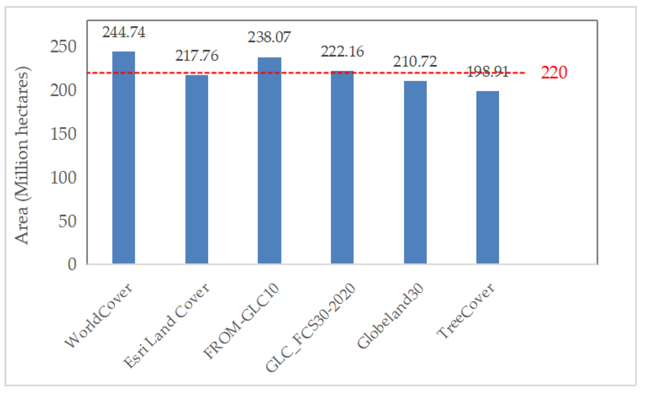
According to data from the Food and Agriculture Organization of the United Nations (FAO) (https://www.fao.org/forest-resources-assessment/2020/en/, accessed on 7 April 2023), the Chinese forest area is about 220 million hectares, accounting for 5% of the world’s total forest area. We compared the area of six products in China, as shown in Figure 2. There are many limitations to the use of a single dataset to represent forest cover. In terms of forest area, the GLC_FCS30-2020 and Esri land cover datasets are closest to the statistical forest area of China. WorldCover and FROM-GLC10 overestimate China’s forest reserves, while GlobeLand30 and TreeCover underestimate the forest area of China. The statistical area reflects the forest area of each dataset but does not accurately represent the accuracy of each dataset.

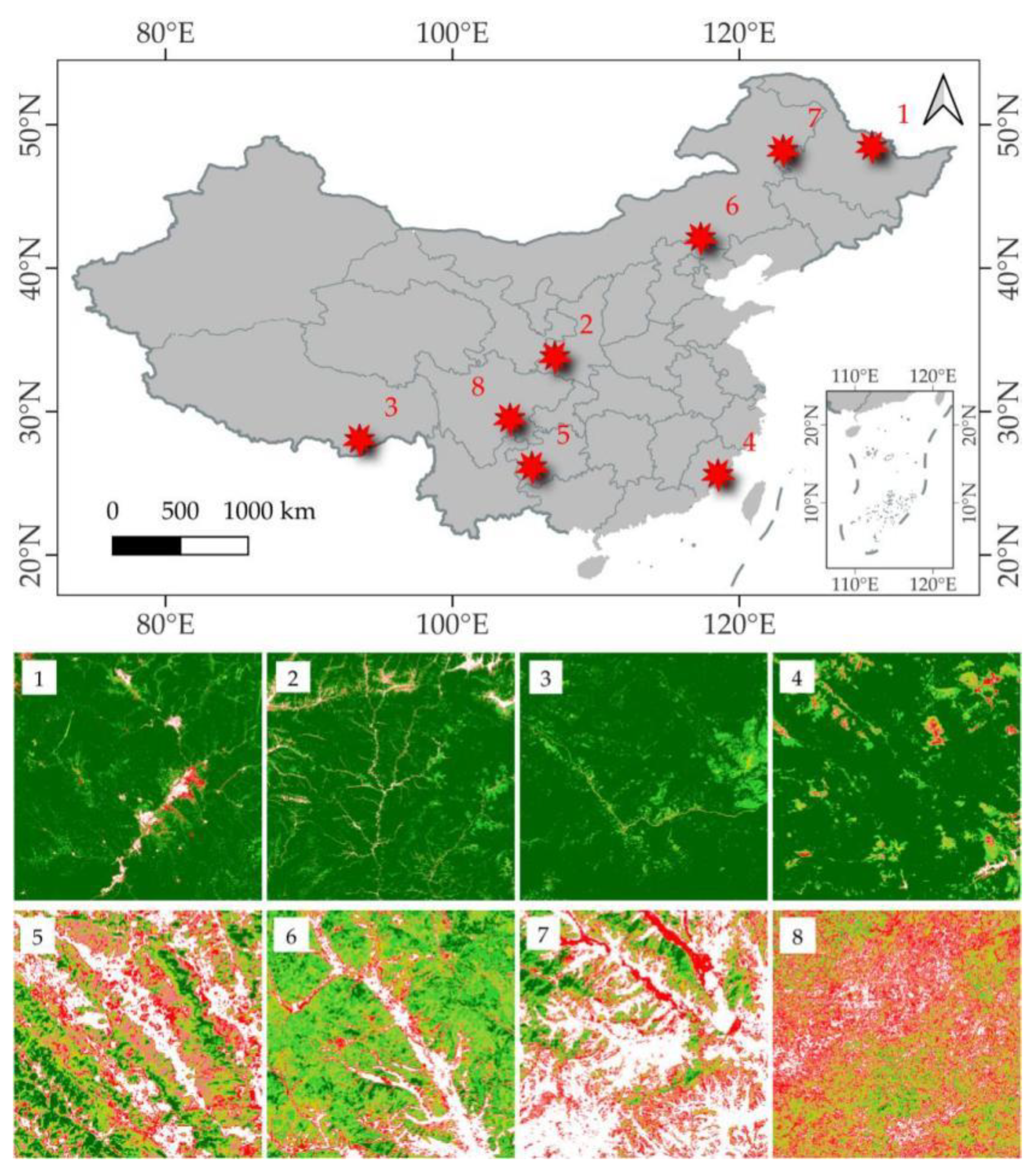
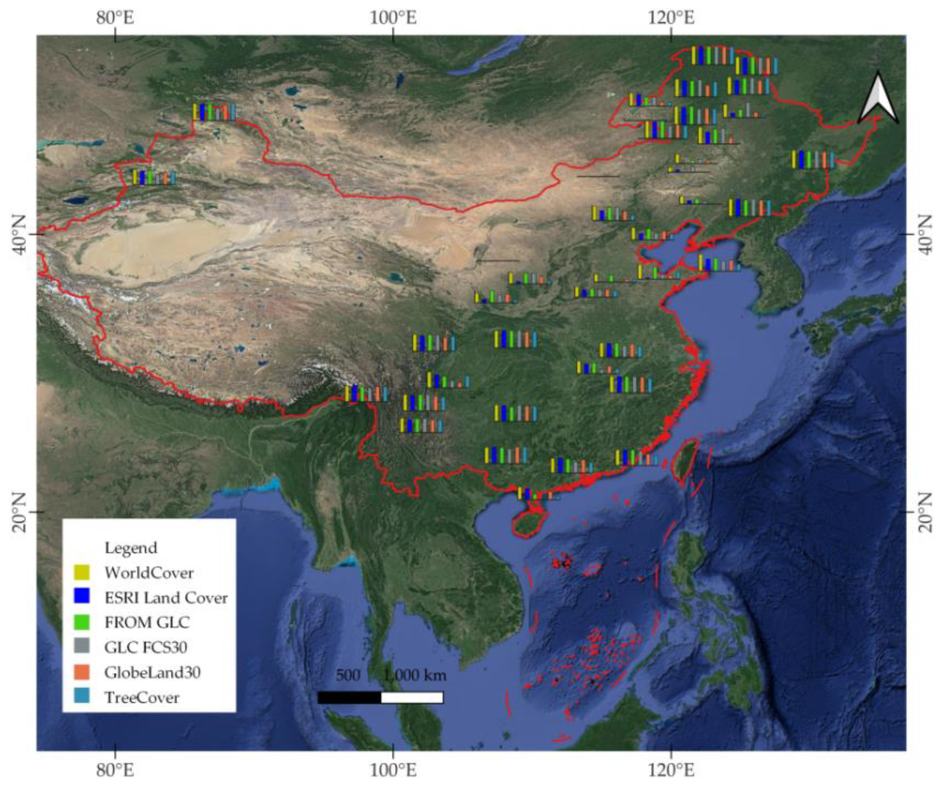
Chinese forests are mainly centered in the northeast, southwest, and vast southern parts of China. These forest datasets exhibit a consistent spatial distribution but a significant spatial inconsistency, as displayed in Figure 3. Northeastern China and the southern Qinghai-Tibet Plateau show a strong spatial consistency, as pictured in Figure 4(1),(3), respectively. These areas (Figure 4(1)–(4)) share some characteristics in common, such as a wider distribution of forests and a high forest cover, even up to 60% [37].

For regions with a complex land cover such as the Yunnan-Guizhou plateau (Figure 4 and Figure 5) and the Sichuan basin (Figure 4, Figure 5, Figure 6, Figure 7 and Figure 8), large spatial inconsistency is presented among these datasets. The spatial consistency is weakest for plain, forest transition areas (Figure 4, Figure 5, Figure 6 and Figure 7) and plantation forest areas (Figure 4, Figure 5 and Figure 6).

4.2. Spatial Consistency Analysis

The areas of different consistency were counted, as shown in Figure 5. The area with the highest consistency is about 126.52 million hectares, accounting for 39.95% of the total area of forest classified (AFC), which is much higher than other areas. However, areas with lower consistency still occupy a large proportion of the AFC. For example, the total area of the area with the consistency of 1 is 52.80 million hectares, accounting for 16.67% of the AFC area.

Statistical analysis was further conducted on the samples located in different consistency regions, as shown in Figure 6. It shows that the higher the consistency area is, the higher the proportion of forest sample points is, which means the higher the probability of the zones being classified correctly. In particular, the regions with consistency ≥5 yielded an accuracy of more than 90%. However, there are still forests not classified by any dataset. It can be inferred from Figure 5 and Figure 6 that the UA with a consistency ≥5 exceeds 90%. With an area of approximately 180 million hectares, these areas exceed 55% of the AFC. Areas with a consistency of 4 or higher exceed 80% UA, with these areas covering approximately 210 million hectares.

The obtained samples were employed to evaluate the accuracy of six forest datasets. The quantification results are summarized in

Table 5. Summary of accuracies of different forest datasets in China.

Datasets	Kappa (%)	OA (%)	PA (%)	UA (%)	F1 Score (%)
WorldCover	82.36	91.62	91.40	87.09	89.19
Esri Land Cover	78.50	90.02	83.38	89.54	86.35
FROM-GLC10	78.40	89.85	86.28	86.82	86.55
GLC_FCS30-2020	76.08	88.79	84.26	85.85	85.05
GlobeLand30	73.80	87.86	80.16	86.75	83.32
TreeCover	69.62	86.20	73.04	88.47	80.01

. WorldCover achieved high accuracies, with Kappa, OA, and F1 reaching 82.36%, 91.62%, and 89.19%, respectively, followed by FROM GLC and Esri Land Cover. However, the forest-related layer in WorldCover is tree cover, which might not be used to represent forest cover accurately. The updated TreeCover exhibits lower accuracy. It might be inappropriate to update TreeCover2000 with “lossyear” and “gain” to represent tree cover of other years. As it is noted with the authors that “The integrated use of version 1.0 2000–2012 data and updated version 1.9 2011–2021 data should be performed with caution”. In general, the accuracy of the 10m resolution dataset is higher than that of the 30m resolution dataset. The F1 score of the 10m resolution dataset is more than 85%, the highest is WorldCover, and the lowest is Esri Land Cover with 86.35%.

The accuracy of selected forest datasets in different regions is illustrated in Figure 7. There is a marked divergence in the forest/non-forest distinction ability of each dataset in different regions. The comparison between Figure 3 and Figure 7 shows that the accuracy tends to be higher in regions with higher consistency and lower in places with poorer forest consistency.

5. Discussions

5.1. Validity of Sampling Strategy and Label Initialization

5.1.1. The Comparison of Sampling Strategies

It is important to note that the distribution of sample points may tend to match the reference datasets. Therefore, it is not possible to generate sample points with reference to a single dataset. Both completely random sampling (CRS) and proportional stratified random sampling (PSRS) are chosen as comparison methods to compare different sampling methods. The map where forest/non-forest areas are the union/intersection of forest in six datasets is used for proportional stratified sampling.

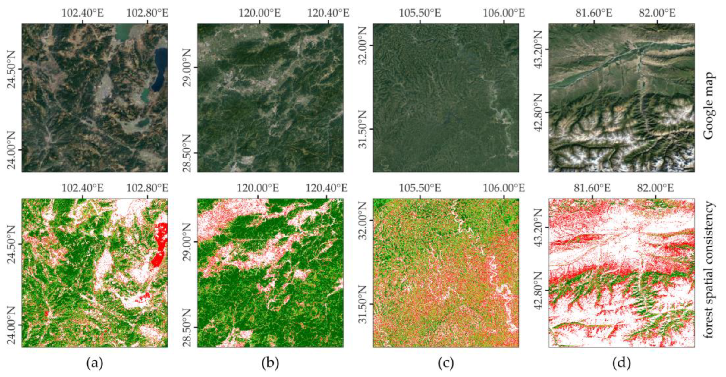
Four regions (as shown in Figure 8) with different spatial distribution patterns of forest distribution are selected to compare different sampling strategies. The statistical pattern is illustrated in Figure 9. The region (b) displays the most consistent forest coverage, followed by the region (a), while the region (c) shows the lowest consistency. The region (d) contains a large proportion of low-consistency areas.

The sample points were mapped to the SCL of forest, and the statistical pattern is displayed in Figure 10. The forest consistency distribution showed the biggest deviation with CRS, followed by PSRS. These two sampling methods are random in nature and cannot control the distribution of samples over different spatially consistent areas. However, the ASRS method produces sample points that closely align with the spatial distribution of forest consistency because it takes into account the different consistency areas. Therefore, the sample points obtained by ASRS are the most in accordance with the forest consistent distribution pattern.

5.1.2. The Comparison of Label Initialization

The relationship between samples and spatial consistency is reported in Figure 11. As illustrated in Figure 11a, 48.2% of the samples are from non-forest areas and more than 50% of the samples are from forest areas with different consistencies. Over 10% of the sample labels were determined by low consistent regions if the initial labels were determined by the reference maps. Although the forest classification accuracy is lower for low-consistency areas, the influence of these areas on the initial labels is significant. Following the initial label assignment design (Figure 11a), 61.86% of the sample initial labels were affected by non-forest, while the other nearly 40% were affected by forest. The results demonstrate that the higher the spatial consistency, the greater the influence on the initial labels.

Additionally, the accuracy of the initial label assignment was calculated, as shown in

Table 6. Summary of accuracies with different labeling methods.

	OA	Forest Accuracy	Non-Forest Accuracy
Forest label with referenced maps (%)	84.48	71.89	98.77
Forest label with sampling strategy (%)	93.24	90.73	94.78

. The initial label design sacrifices the small accuracy of non-forest samples (by 3.99%) to significantly boost the accuracy of forest samples (by 18.84%). Overall, the OA of labeling with the proposed design is 93.24%, which is 8.76% higher than that of labeling with forest datasets. This demonstrates that it is effective and efficient to comprehensively take into account the probability of different classes at the same location to determine the sample labels. The proposed design dramatically promotes the accuracy of the initial labels and greatly reduces the workload of manually modifying the samples.

5.2. Reasons for Inconsistency across Forest Datasets

(1) Differences in FRC definition between forest datasets

The FRCs of medium-resolution forest-related datasets listed in this paper vary significantly in their definitions. The FRCs in the four datasets of GlobeLand30, GLC_FCS30-2020, and FROM-GLC10 are named “forest” and are constrained by different criteria of tree height, vegetation cover, and other uses. In contrast, the FRCs in WorldCover, Esri Land Cover, and TreeCover are named “trees/tree cover” and are constrained by tree height or the proportion of area. Due to the variations in definitions, the objects focused on might differ widely.

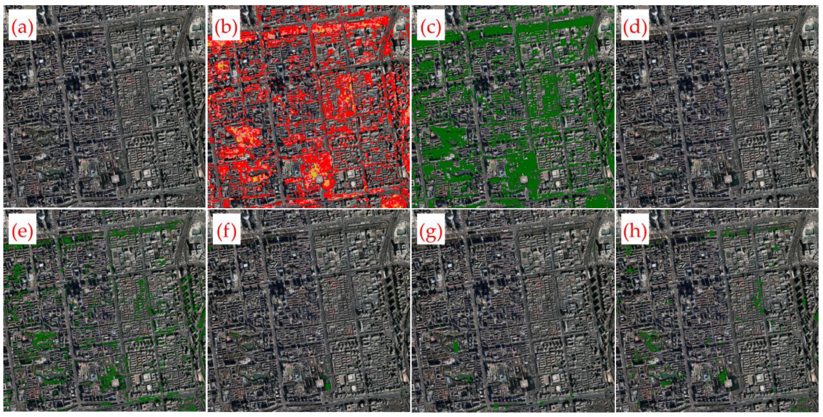
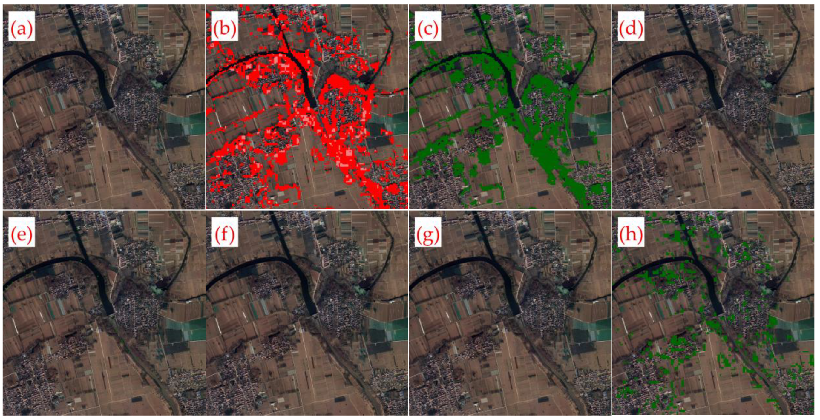
Theoretically, when using datasets with the FRC definition as “trees/tree cover” to describe forest distribution is prone to more misclassification errors. It means that these datasets regard trees without satisfying the forest scale as forest. Although part of the misclassified pixels can be removed by area constraints, this does not solve the problem completely, especially for green belts around cities (Figure 12) or villages (Figure 13).

Although the FRC is strictly defined in LULC datasets, the results appear to be inconsistent with the definitions. As shown in Figure 12, this site is located in an urban area, dominated by dense buildings and roads. WorldCover contributes the most to the forest consistency of this area, followed by FROM GLC10. The FRC in WorldCover is “Tree cover”, defined as a geographic area dominated by trees with an area of 10% or more. However, this area (Figure 12c) does not belong to the “Tree cover” according to the definition. The FRC in FROM_GLC10 is “forest”, and there is a discrepancy between the definition and the result (Figure 12e).

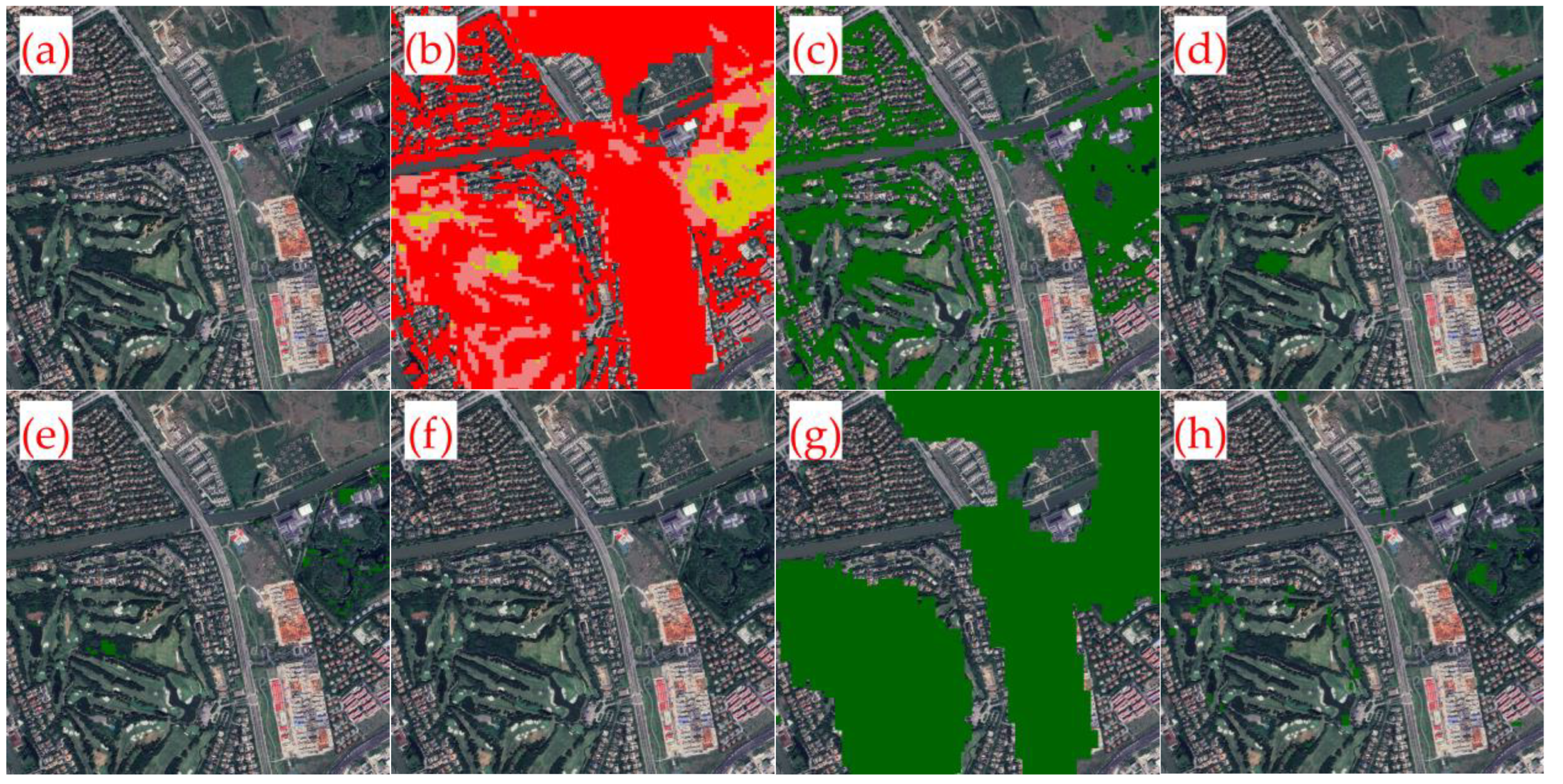
Similar to Figure 12, Figure 14 is located in an urban area. Despite the slight discrepancy with the definition, the WorldCover results are in agreement with the “trees” in this region (Figure 14c). In comparison, Esri Land Cover (Figure 14d) and TreeCover (Figure 14h) do not provide a good result for “trees”. In GlobeLand30, the FRC is “forest”, yet there is a significant error in the results with grass/crop misclassified as forest.

(2) Data sources

Satellite remote sensing images are still the main source in forest mapping, especially at large scales (e.g., a global scale). Remote sensing images directly influence the classification results. On the one hand, the data sources of datasets involved are different, including differences in sensors and time. It is difficult to keep the temporal consistency of the images used in different datasets, even if they come from the same sensor for the same year. On the other hand, remote sensing images are limited. Scholars usually constrain the definition of forest with usage or thresholds of vegetation cover, tree height, and area. However, there is a lack of auxiliary data for some attributes, which are also difficult to measure in remotely sensed images, such as tree height and use.

Furthermore, the quality of remote sensing images impacts the classification accuracy severely. The acquisition of remote sensing images is heavily affected by weather, especially in low latitudes and coastal areas that are strongly influenced by a monsoon climate. Poorer-quality images suffer the most in classification accuracy. The discontinuous transition is one of the most remarkable forms of image impact, as shown in Figure 15.

(3) Spatial positioning error/geometric error

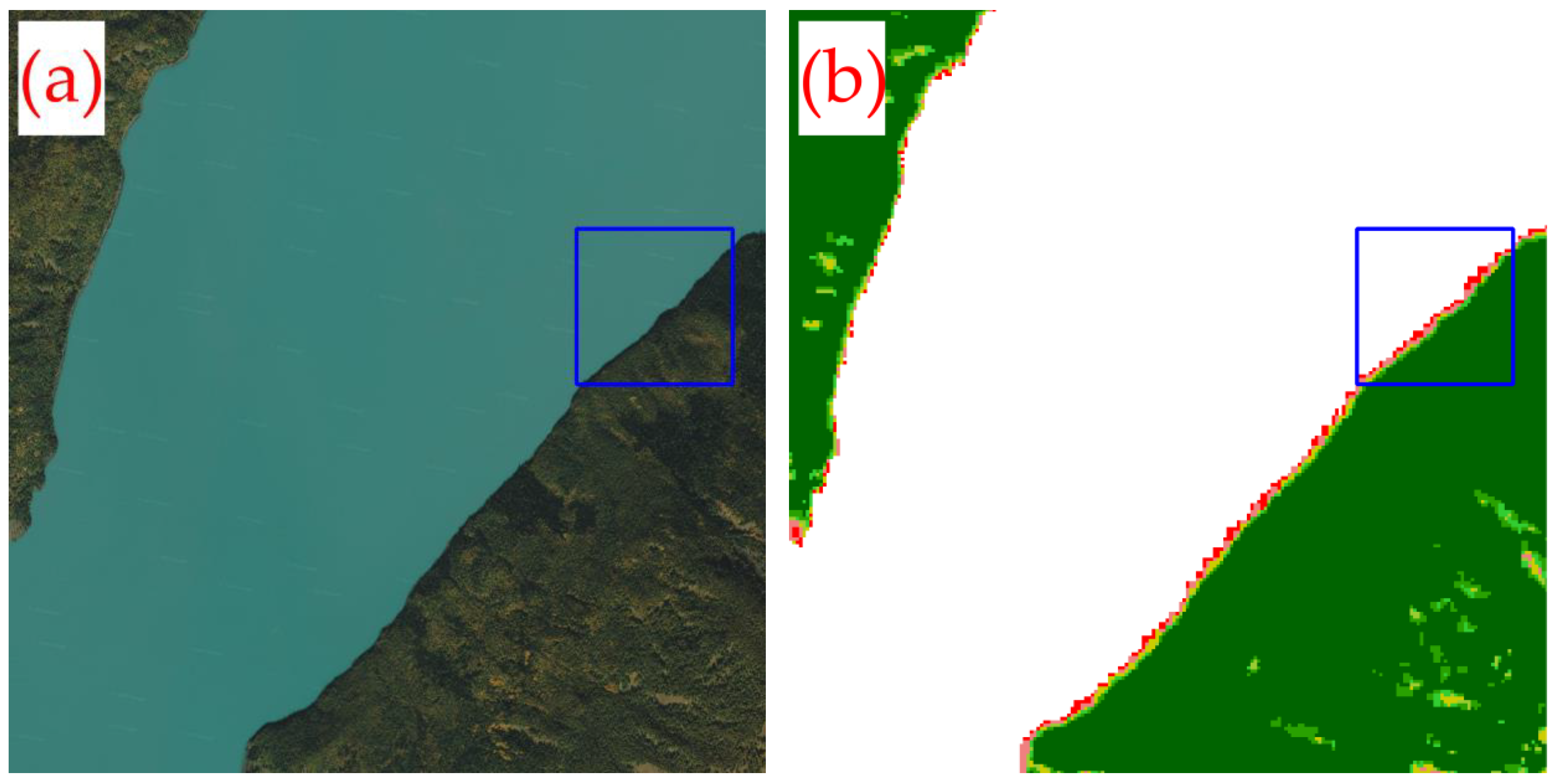
The lack of satellite imagery in the datasets makes it difficult to estimate the consequences of geometric errors on the inconsistency of forest datasets. It is also a challenge to capture such errors due to the homogeneity within forest areas. However, this difference, which might be caused by geometric error, is noticeable in the boundary of the forest, especially at the junction of the forest and the river.

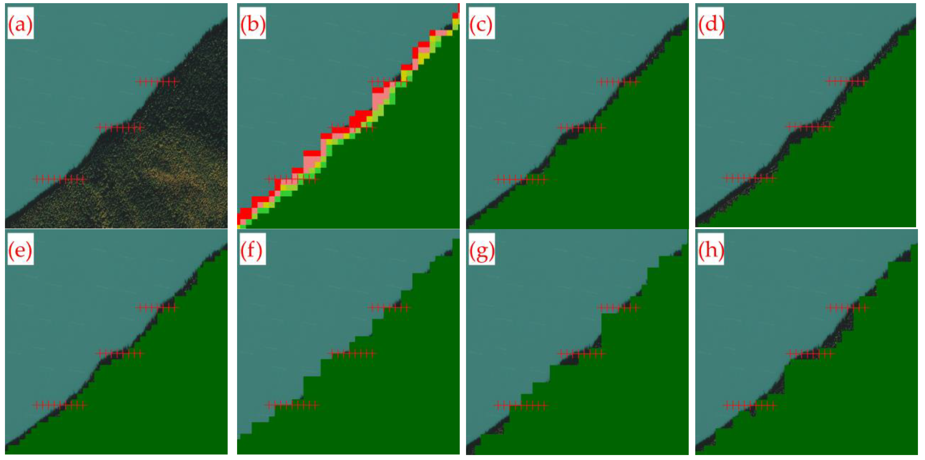
As shown in Figure 16, the forest and water are directly adjacent to each other in this area via comparison with the high-resolution map. Such errors might be introduced by mixed pixels and classification algorithms. However, it is speculated that such errors are caused by the geometric error of the remotely sensed images. Figure 17 represents the details of the blue area in Figure 13. The 10m resolution data is superior to the 30m resolution data in terms of spatial detail representation. There is a visible discrepancy between the results of the 10m- and the 30m-resolution datasets at the forest boundary.

5.3. Limitations of Point-Based Accuracy Metrics

Sample point-based accuracy evaluation is commonly used in medium-resolution LULC classification. However, are such metrics an absolute criterion for classification accuracy? Based on the forest datasets, this question is discussed in this section.

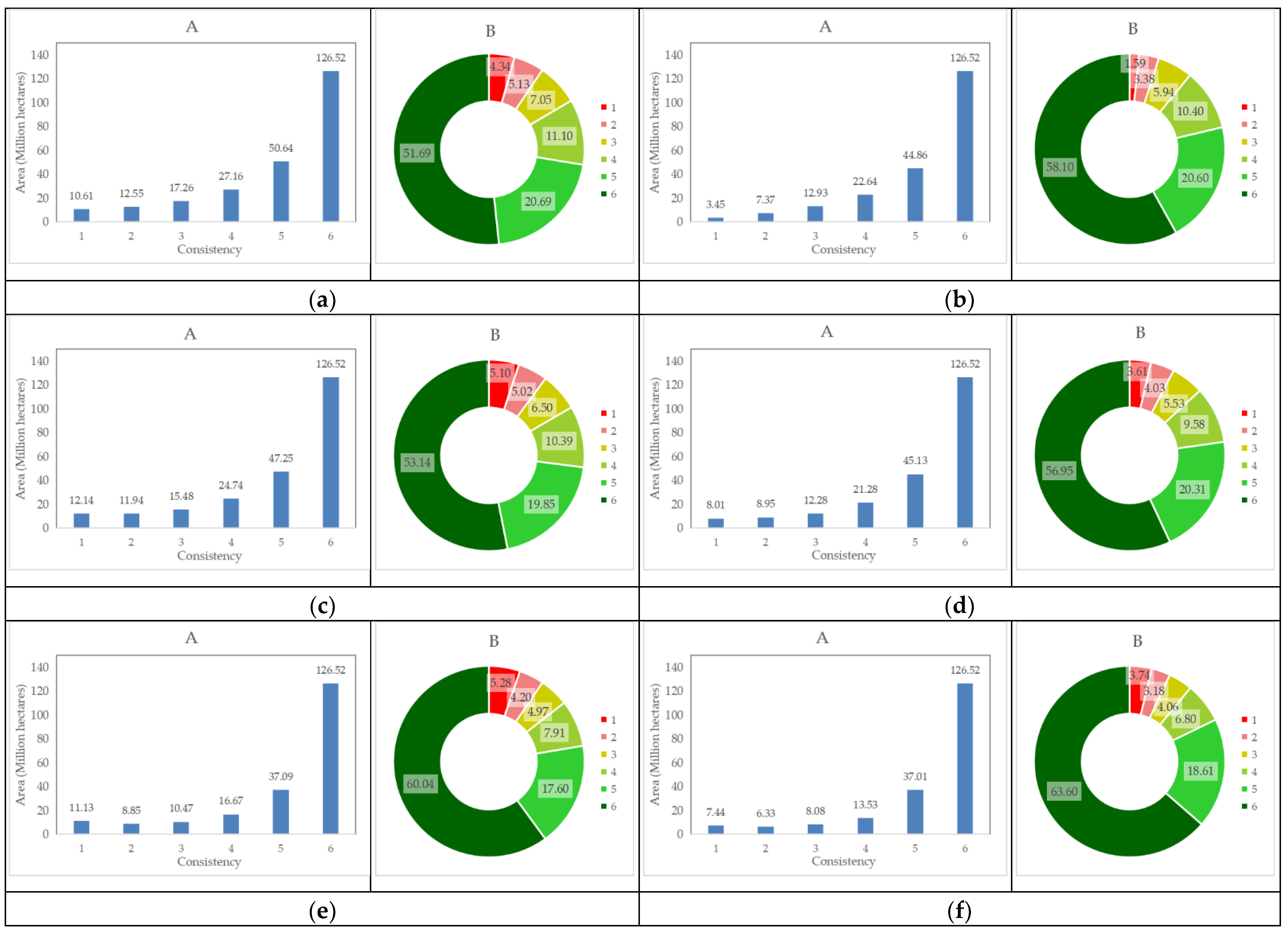
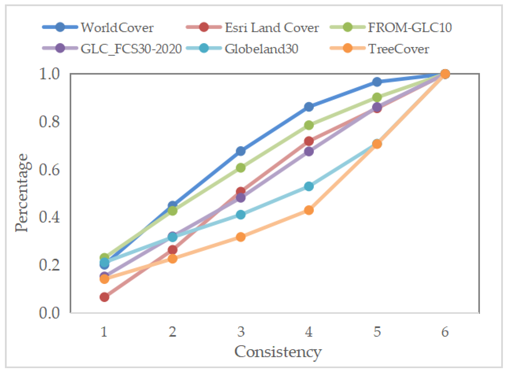
The correlations of forest consistency with these datasets are further tallied as shown in Figure 18. The relationships show similar characteristics, i.e., the higher the consistency, the larger the area shared. Esri land cover shows the lowest proportion of low consistency (≤2) area. Esri land cover has the smallest percentage of low consistency area, while WorldCover, FROM-GLC10, and GLC_FCS30 are larger. The proportion of the high consistency (≥5) area of TreeCover is 82.21%, which is higher than other datasets.

Theoretically, areas with higher spatial consistency show higher accuracy, which means higher reliability. Taking TreeCover as an example, by comparing Figure 18 and Table 5, it is clear that the metrics are lower despite the fact that TreeCover has a high proportion of high-consistency regions in these datasets.

The contribution of TreeCover to different forest consistency regions is demonstrated in Figure 19. For example, the contribution of TreeCover to the region with consistency ≥5 is about 70%, which means that the intersection with TreeCover in this region accounts for 70% of the total area. The sample selection within this region is random. Consequently, about 70% of the points in the region with consistency ≥5 are located in the forested region of TreeCover, while 30% fall in the non-forested region. This gives rise to errors.

Furthermore, sample selection affects the accuracy metrics tremendously. It is challenging to estimate the pixel-level error of forest datasets due to the influence of images, geometric accuracy, forest definitions, and classification schemes. It seems that metrics could not be used as the exclusive criteria for evaluating medium-resolution datasets. As a result, the accuracy indicators do not provide the absolute accuracy of forest datasets, which might only be used as a reference for the perception and use of the available datasets.

5.4. Reflections on the Future of Forest Research

Although each dataset exhibited high accuracies, there were remarkable spatial inconsistencies between different datasets. In areas with dense forests and high forest cover, the forest datasets showed better spatial consistency and higher accuracy. On the contrary, in areas with complex land cover and fragmented forests, the forest datasets present worse spatial consistency and lower accuracy. The accuracy of each product was lower in areas with small forest areas, the transition zone between forest and non-forest, and plantation forests. Generally speaking, the higher the consistency, the higher the accuracy of the forest. Therefore, the spatial consistency can accurately reflect the difficulty of forest extraction regionally.

These datasets provide important first-hand knowledge for forest study. On the one hand, it is possible to synthesize existing forest datasets by multivariate data fusion to generate higher-precision forest datasets. It is effective to use existing LULC products by majority voting or weighted averaging [14]. Based on three LULC products, Xu et al. [38] synthesized the 2015 global surface coverage results via Dempster-Shafer’s theory. On the other hand, high-precision samples are vital to the training and validation of forest classification [5,39]. It is necessary to take advantage of existing LULC products to direct sample selection, especially where areas have poor consistency. Through additional experimentation, we have discovered that the highly consistent region of the forest can serve as a direct sample for forest classification.

Furthermore, improvement can be introduced to the LULC classification methods. Machine learning is mostly used for medium-resolution LULC classification nowadays, especially the random forest algorithm. Recently, scholars have explored a lot of deep learning in applying medium-resolution remote sensing images, such as forest classification [40] and LULC classification [41,42]. Deep learning is superior in capturing spatial details and texture. However, deep learning still has many challenges in medium-resolution forest classification because of resolution limitations and the characteristics of the forest. Therefore, it is important to understand how to put more effort into focusing on spectra in the absence of texture information. In addition, we found that large reception fields have a negative influence on the forest classification using medium-resolution remote sensing images.

6. Conclusions

In this paper, a detailed review and assessment is carried out on six forest-related global LULC datasets around 2020, including WorldCover, Esri land cover, GlobeLand30, GLC FCS30, FROM GLC10, and TreeCover. The results show that these datasets exhibit high accuracies, with OA exceeding 85%. However, these datasets suffer from large spatial inconsistencies. More than 25% of the areas show an accuracy of less than 15% while areas of high consistency (≥5) with >90% accuracy account for only 56.49% of the AFC. The high-consistency areas, therefore, comprise the majority of the forest area. The low- to medium-consistency areas, which were difficult to accurately classify, will be the key to the reliability of the datasets. Extra attention to typical low-consistency areas (such as areas with complex topography, forest fragmentation, forest transition zones, and plantation) would likely be useful to improve forest classification accuracy. This study thoroughly evaluates the accuracy and reliability of regional forest-related datasets for China in 2020. It provides an important reference for the rational use of these datasets and the improvements of future forest studies.

References

1. Campbell, J.B.; Wynne, R.H. Introduction to Remote Sensing; Guilford Press: New York, NY, USA, 2011. [Google Scholar]
2. Reinhold, A.; Wolff, G. Methods of representing the results of photo interpretation. Photogrammetria 1970, 25, 201–207. [Google Scholar] [CrossRef]
3. France, M.; Hedges, P. A hydrological comparison of Landsat TM, Landsat MSS and black & white aerial photography. In Proceedings of the Remote Sensing for Ressources Development and Environmental Management. International Symposium, Enschede, The Netherlands, 25–29 August 1986; 1986; Volume 7, pp. 717–720. [Google Scholar]
4. Kangas, A.; Maltamo, M. Forest Inventory: Methodology and Applications; Springer Science & Business Media: Berlin/Heidelberg, Germany, 2006; Volume 10. [Google Scholar]
5. Zhang, X.; Long, T.; He, G.; Guo, Y.; Yin, R.; Zhang, Z.; Xiao, H.; Li, M.; Cheng, B. Rapid generation of global forest cover map using Landsat based on the forest ecological zones. J. Appl. Remote Sens. 2020, 14, 022211. [Google Scholar] [CrossRef]
6. Belgiu, M.; Drăguţ, L. Random forest in remote sensing: A review of applications and future directions. ISPRS J. Photogramm. Remote Sens. 2016, 114, 24–31. [Google Scholar] [CrossRef]
7. Gigović, L.; Pourghasemi, H.R.; Drobnjak, S.; Bai, S. Testing a New Ensemble Model Based on SVM and Random Forest in Forest Fire Susceptibility Assessment and Its Mapping in Serbia’s Tara National Park. Forests 2019, 10, 408. [Google Scholar] [CrossRef]
8. Peng, X.; He, G.; She, W.; Zhang, X.; Wang, G.; Yin, R.; Long, T. A Comparison of Random Forest Algorithm-Based Forest Extraction with GF-1 WFV, Landsat 8 and Sentinel-2 Images. Remote Sens. 2022, 14, 5296. [Google Scholar] [CrossRef]
9. White, J.C.; Coops, N.C.; Wulder, M.A.; Vastaranta, M.; Hilker, T.; Tompalski, P. Remote Sensing Technologies for Enhancing Forest Inventories: A Review. Can. J. Remote Sens. 2016, 42, 619–641. [Google Scholar] [CrossRef]
10. Di Biase, R.M.; Fattorini, L.; Marchi, M. Statistical inferential techniques for approaching forest mapping. A review of methods. Ann. Silvic. Res. 2018, 42, 46–58. [Google Scholar]
11. Banskota, A.; Kayastha, N.; Falkowski, M.J.; Wulder, M.A.; Froese, R.E.; White, J.C. Forest Monitoring Using Landsat Time Series Data: A Review. Can. J. Remote Sens. 2014, 40, 362–384. [Google Scholar] [CrossRef]
12. Shimada, M.; Itoh, T.; Motooka, T.; Watanabe, M.; Shiraishi, T.; Thapa, R.; Lucas, R. New global forest/non-forest maps from ALOS PALSAR data (2007–2010). Remote Sens. Environ. 2014, 155, 13–31. [Google Scholar] [CrossRef]
13. Liu, L.; Zhang, X.; Gao, Y.; Chen, X.; Shuai, X.; Mi, J. Finer-Resolution Mapping of Global Land Cover: Recent Developments, Consistency Analysis, and Prospects. J. Remote Sens. 2021, 2021, 5289697. [Google Scholar] [CrossRef]
14. Venter, Z.S.; Barton, D.N.; Chakraborty, T.; Simensen, T.; Singh, G. Global 10 m Land Use Land Cover Datasets: A Comparison of Dynamic World, World Cover and Esri Land Cover. Remote Sens. 2022, 14, 4101. [Google Scholar] [CrossRef]
15. Wang, J.; Yang, X.; Wang, Z.; Cheng, H.; Kang, J.; Tang, H.; Li, Y.; Bian, Z.; Bai, Z. Consistency Analysis and Accuracy Assessment of Three Global Ten-Meter Land Cover Products in Rocky Desertification Region—A Case Study of Southwest China. ISPRS Int. J. Geo-Inf. 2022, 11, 202. [Google Scholar] [CrossRef]
16. Ding, Y.; Yang, X.; Wang, Z.; Fu, D.; Li, H.; Meng, D.; Zeng, X.; Zhang, J. A Field-Data-Aided Comparison of Three 10 m Land Cover Products in Southeast Asia. Remote Sens. 2022, 14, 5053. [Google Scholar] [CrossRef]
17. Sun, W.; Ding, X.; Su, J.; Mu, X.; Zhang, Y.; Gao, P.; Zhao, G. Land use and cover changes on the Loess Plateau: A comparison of six global or national land use and cover datasets. Land Use Policy 2022, 119, 106165. [Google Scholar] [CrossRef]
18. Wang, H.; Yan, H.; Hu, Y.; Xi, Y.; Yang, Y. Consistency and Accuracy of Four High-Resolution LULC Datasets—Indochina Peninsula Case Study. Land 2022, 11, 758. [Google Scholar] [CrossRef]
19. Xu, Y.; Yu, L.; Feng, D.; Peng, D.; Li, C.; Huang, X.; Lu, H.; Gong, P. Comparisons of three recent moderate resolution African land cover datasets: CGLS-LC100, ESA-S2-LC20, and FROM-GLC-Africa30. Int. J. Remote Sens. 2019, 40, 6185–6202. [Google Scholar] [CrossRef]
20. Congalton, R.; Gu, J.; Yadav, K.; Thenkabail, P.; Ozdogan, M. Global Land Cover Mapping: A Review and Uncertainty Analysis. Remote Sens. 2014, 6, 12070–12093. [Google Scholar] [CrossRef]
21. Shi, W.; Zhao, X.; Zhao, J.; Zhao, S.; Guo, Y.; Liu, N.; Sun, N.; Du, X.; Sun, M. Reliability and consistency assessment of land cover products at macro and local scales in typical cities. Int. J. Digit. Earth 2023, 16, 486–508. [Google Scholar] [CrossRef]
22. Dong, S.; Guo, H.; Chen, Z.; Pan, Y.; Gao, B. Spatial Stratification Method for the Sampling Design of LULC Classification Accuracy Assessment: A Case Study in Beijing, China. Remote Sens. 2022, 14, 865. [Google Scholar] [CrossRef]
23. Galiatsatos, N.; Donoghue, D.N.M.; Watt, P.; Bholanath, P.; Pickering, J.; Hansen, M.C.; Mahmood, A.R.J. An Assessment of Global Forest Change Datasets for National Forest Monitoring and Reporting. Remote Sens. 2020, 12, 1790. [Google Scholar] [CrossRef]
24. Feng, M.; Sexton, J.O.; Huang, C.; Anand, A.; Channan, S.; Song, X.-P.; Song, D.-X.; Kim, D.-H.; Noojipady, P.; Townshend, J.R. Earth science data records of global forest cover and change: Assessment of accuracy in 1990, 2000, and 2005 epochs. Remote Sens. Environ. 2016, 184, 73–85. [Google Scholar] [CrossRef]
25. Hao, X.; Luo, S.; Che, T.; Wang, J.; Li, H.; Dai, L.; Huang, X.; Feng, Q. Accuracy assessment of four cloud-free snow cover products over the Qinghai-Tibetan Plateau. Int. J. Digit. Earth 2018, 12, 375–393. [Google Scholar] [CrossRef]
26. Zhang, C.; Dong, J.; Ge, Q. Quantifying the accuracies of six 30-m cropland datasets over China: A comparison and evaluation analysis. Comput. Electron. Agric. 2022, 197, 106946. [Google Scholar] [CrossRef]
27. Zanaga, D.; Van De Kerchove, R.; De Keersmaecker, W.; Souverijns, N.; Brockmann, C.; Quast, R.; Wevers, J.; Grosu, A.; Paccini, A.; Vergnaud, S.; et al. ESA WorldCover 10 m 2020 v100. 2021. Available online: https://zenodo.org/record/5571936#.Y0uZbnZBxaQ (accessed on 7 April 2023).
28. Karra, K.; Kontgis, C.; Statman-Weil, Z.; Mazzariello, J.C.; Mathis, M.; Brumby, S.P. Global land use/land cover with Sentinel 2 and deep learning. In Proceedings of the 2021 IEEE International Geoscience and Remote Sensing Symposium IGARSS, Brussels, Belgium, 11–16 July 2021; pp. 4704–4707. [Google Scholar]
29. Gong, P.; Liu, H.; Zhang, M.; Li, C.; Wang, J.; Huang, H.; Clinton, N.; Ji, L.; Li, W.; Bai, Y.; et al. Stable classification with limited sample: Transferring a 30-m resolution sample set collessscted in 2015 to mapping 10-m resolution global land cover in 2017. Sci. Bull. 2019, 64, 370–373. [Google Scholar] [CrossRef] [PubMed]
30. Chen, J.; Chen, J.; Liao, A.; Cao, X.; Chen, L.; Chen, X.; He, C.; Han, G.; Peng, S.; Lu, M.; et al. Global land cover mapping at 30m resolution: A POK-based operational approach. ISPRS J. Photogramm. Remote Sens. 2015, 103, 7–27. [Google Scholar] [CrossRef]
31. Jun, C.; Ban, Y.; Li, S. Open access to Earth land-cover map. Nature 2014, 514, 434. [Google Scholar] [CrossRef]
32. Zhang, X.; Liu, L.; Chen, X.; Gao, Y.; Xie, S.; Mi, J. GLC_FCS30: Global land-cover product with fine classification system at 30 m using time-series Landsat imagery. Earth Syst. Sci. Data 2021, 13, 2753–2776. [Google Scholar] [CrossRef]
33. Hansen, M.C.; Potapov, P.V.; Moore, R.; Hancher, M.; Turubanova, S.A.; Tyukavina, A.; Thau, D.; Stehman, S.V.; Goetz, S.J.; Loveland, T.R.; et al. High-resolution global maps of 21st-century forest cover change. Science 2013, 342, 850–853. [Google Scholar] [CrossRef]
34. Zhang, X.; Liu, L.; Chen, X.; Xie, S.; Gao, Y. Fine Land-Cover Mapping in China Using Landsat Datacube and an Operational SPECLib-Based Approach. Remote Sens. 2019, 11, 1056. [Google Scholar] [CrossRef]
35. Zhang, X.; Liu, L.; Zhao, T.; Gao, Y.; Chen, X.; Mi, J. GISD30: Global 30 m impervious-surface dynamic dataset from 1985 to 2020 using time-series Landsat imagery on the Google Earth Engine platform. Earth Syst. Sci. Data 2022, 14, 1831–1856. [Google Scholar] [CrossRef]
36. Gong, P.; Wang, J.; Yu, L.; Zhao, Y.; Zhao, Y.; Liang, L.; Niu, Z.; Huang, X.; Fu, H.; Liu, S.; et al. Finer resolution observation and monitoring of global land cover: First mapping results with Landsat TM and ETM+ data. Int. J. Remote Sens. 2012, 34, 2607–2654. [Google Scholar] [CrossRef]
37. National Forestry and Grassland Administration. China Forest Resources Report; Chinese Forestry Press: Beijing, China, 2020. [Google Scholar]
38. Xu, X.; Li, B.; Liu, X.; Li, X.; Shi, Q. Mapping annual global land cover changes at a 30 m resolution from 2000 to 2015. Natl. Remote Sens. Bull. 2021, 25, 1896–1916. [Google Scholar] [CrossRef]
39. Zhu, Z.; Gallant, A.L.; Woodcock, C.E.; Pengra, B.; Olofsson, P.; Loveland, T.R.; Jin, S.; Dahal, D.; Yang, L.; Auch, R.F. Optimizing selection of training and auxiliary data for operational land cover classification for the LCMAP initiative. ISPRS J. Photogramm. Remote Sens. 2016, 122, 206–221. [Google Scholar] [CrossRef]
40. Ahmed, N.; Saha, S.; Shahzad, M.; Fraz, M.M.; Zhu, X.X. Progressive Unsupervised Deep Transfer Learning for Forest Mapping in Satellite Image. In Proceedings of the IEEE/CVF International Conference on Computer Vision, Montreal, BC, Canada, 11–17 October 2021; pp. 752–761. [Google Scholar]
41. Yin, R.; He, G.; Wang, G.; Long, T.; Li, H.; Zhou, D.; Gong, C. Automatic Framework of Mapping Impervious Surface Growth With Long-Term Landsat Imagery Based on Temporal Deep Learning Model. IEEE Geosci. Remote Sens. Lett. 2022, 19, 2502605. [Google Scholar] [CrossRef]
42. Xia, L.; Zhao, F.; Chen, J.; Yu, L.; Lu, M.; Yu, Q.; Liang, S.; Fan, L.; Sun, X.; Wu, S.; et al. A full resolution deep learning network for paddy rice mapping using Landsat data. ISPRS J. Photogramm. Remote Sens. 2022, 194, 91–107. [Google Scholar] [CrossRef]
Figure 1. The pre-processed forest datasets. (a) WorldCover 2020, (b) ESRI Land Cover 2020, (c) FROM-GLC10, (d) GLC_FCS30-2020, (e) GlobeLand30 2020, and (f) TreeCover 2020.
Remotesensing 15 02557 g001aRemotesensing 15 02557 g001b
Figure 2. Forest area in China for each dataset.
Remotesensing 15 02557 g002
Figure 3. Spatial consistency of medium-resolution forest datasets.
Remotesensing 15 02557 g003
Figure 4. Spatial consistency of forest datasets in typical areas of China. The high spatial consistency sites (14) are located in Lesser Khingan Mountains, Qinling Mountains, Southeastern Qinghai-Tibet Plateau, and Daiyun Mountain, respectively. The low spatial consistency sites (58) are located in Yunnan-Kweichow Plateau, Mongolian Plateau, Northeast China Plain, and Sichuan Basin.
Remotesensing 15 02557 g004
Figure 5. Statistics of different consistent zones. (a) presents the area of the consistent zones; (b) presents the proportion of the consistent areas to the AFC.
Remotesensing 15 02557 g005
Figure 6. Comparison of different consistency zones. (a) is the number of samples in different consistency zones; (b) is the proportion of forest sample points in different consistency zones.
Remotesensing 15 02557 g006
Figure 7. F1 score for different regions of the six forest datasets.
Remotesensing 15 02557 g007
Figure 8. Four regions with different spatial patterns of forest distribution. Selected regions (ad) scatter in different locations.
Remotesensing 15 02557 g008
Figure 9. The statistical pattern of forest spatial distribution in four regions. The subfigures (ad) correspond to the forest pattern for the four regions (ad) in Figure 8, respectively.
Remotesensing 15 02557 g009
Figure 10. The gap between the distribution of samples and forest consistency. (ad) are samples selected in regions (ad) in Figure 8, respectively.
Remotesensing 15 02557 g010
Figure 11. Relationship between samples and spatial consistency. (a) presents the relationship between sample size and spatial consistency of forest; (b) exhibits the relationship between initial class and spatial consistency of forest.
Remotesensing 15 02557 g011
Figure 12. Performance of forest datasets in urban areas. The high-resolution map in QGIS is shown in (a); (bh) indicates the overlay of the spatial consistency of forest, WorldCover, Esri Land Cover, FROM-GLC10, GLC_FCS30-2020, GlobeLand30, and Tree Cover 2020 on the high-resolution map.
Remotesensing 15 02557 g012
Figure 13. Performance of forest datasets in rural areas. The high-resolution map in QGIS is shown in (a); (bh) indicates the overlay of the spatial consistency of forest, WorldCover, Esri Land Cover, FROM-GLC10, GLC_FCS30-2020, GlobeLand30, and Tree Cover 2020 on the high-resolution map.
Remotesensing 15 02557 g013
Figure 14. The inconsistency between definition and results. The high-resolution map in QGIS is shown in (a); (bh) indicates the overlay of the spatial consistency of forest, WorldCover, Esri Land Cover, FROM-GLC10, GLC_FCS30-2020, GlobeLand30, and Tree Cover 2020 on the high-resolution map.
Remotesensing 15 02557 g014
Figure 15. Incoherent transitions. (a) Esri Land Cover; (bd) FROM GLC10.
Remotesensing 15 02557 g015
Figure 16. Inconsistency caused by spatial location errors. (a) High-resolution map in QGIS; (b) Product consistency map.
Remotesensing 15 02557 g016
Figure 17. Edge differences in forest datasets. The high-resolution map in QGIS is shown in (a); (bh) indicates the overlay of the spatial consistency of forest, WorldCover, Esri Land Cover, FROM-GLC10, GLC_FCS30-2020, GlobeLand30, and Tree Cover 2020 on the high-resolution map.
Remotesensing 15 02557 g017
Figure 18. The relevance between forest datasets and consistency. (af) display the statistical pattern of WorldCover, Esri land cover, FROM-GLC10, GlobeLand30, GLC_FCS30, and TreeCover, respectively. Sub-figure A means the area of different consistency and sub-figure B represent the proportion of the area with different consistency to the total forest area.
Remotesensing 15 02557 g018
Figure 19. Contribution of each dataset to areas with different consistency.
Remotesensing 15 02557 g019