

Exploring the Impact of Grain-for-Green Program on Trade-Offs and Synergies among Ecosystem Services in West Liao River Basin, China

Abstract
1. Introduction
2. Study Area and Data
2.1. Study Area
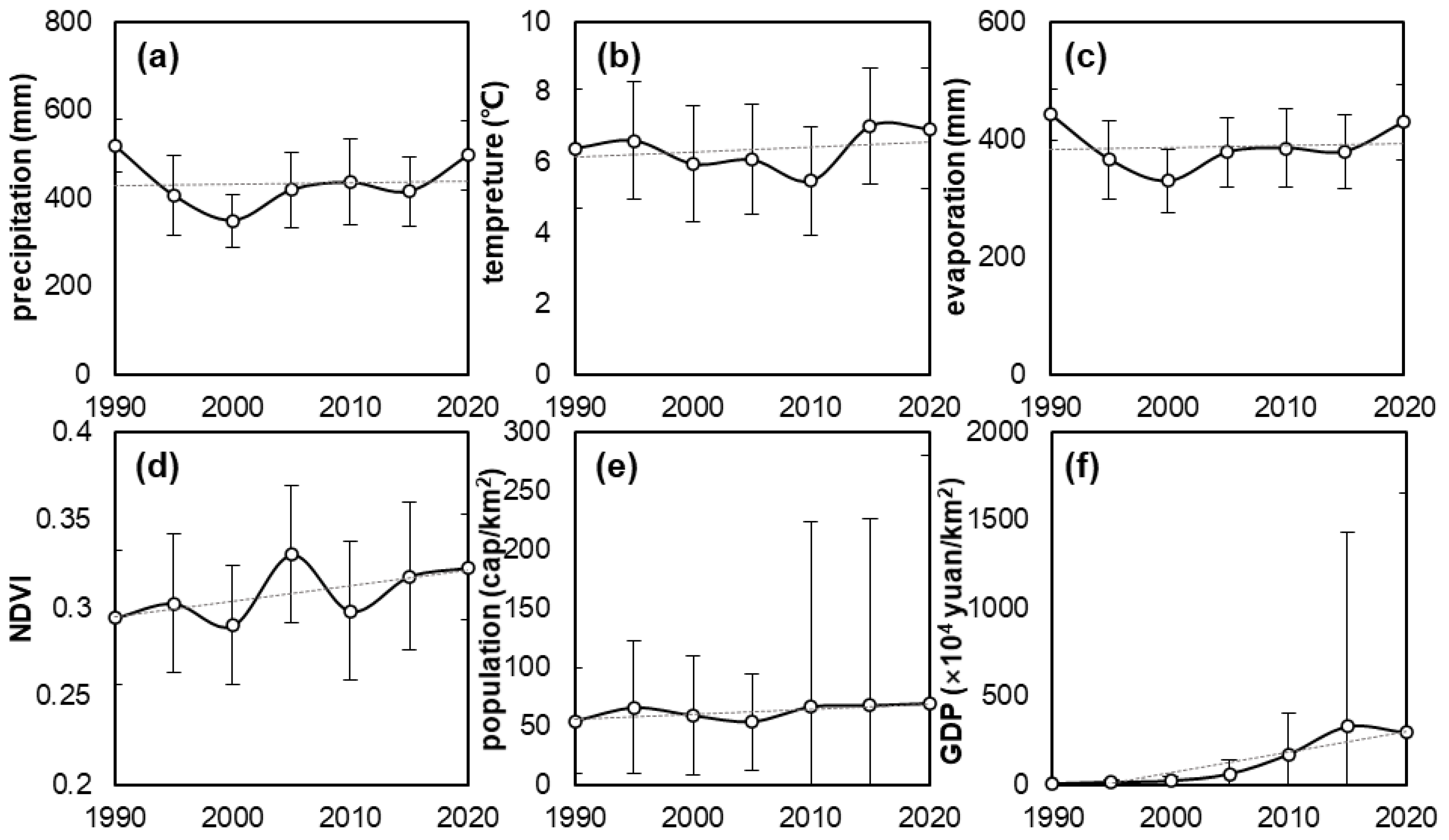
2.2. Data
3. Methods
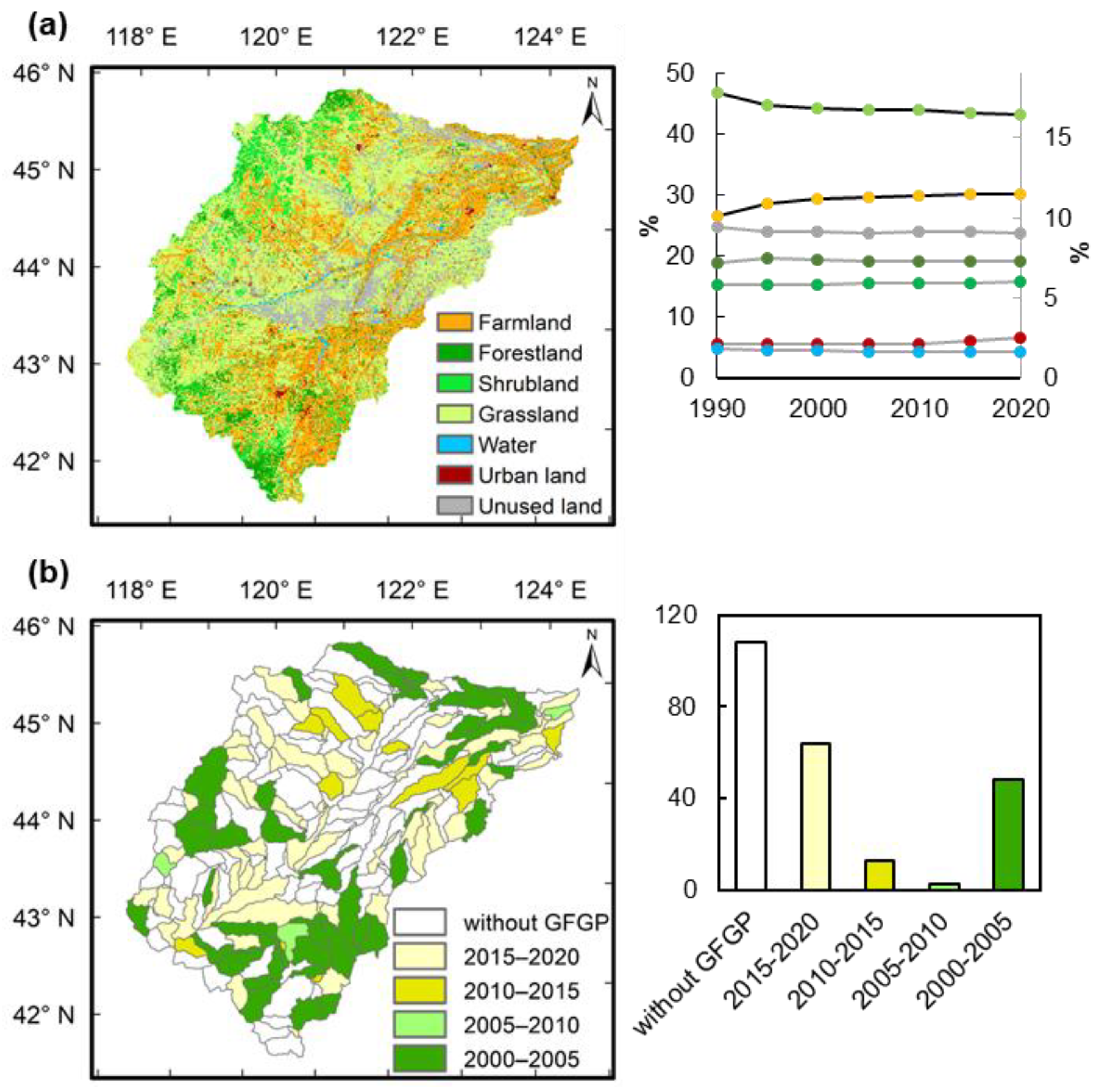
3.1. Landcover Change Detection
3.2. Quantifying Ecosystem Services
3.3. Assessing the Relationship among Ecosystem Services
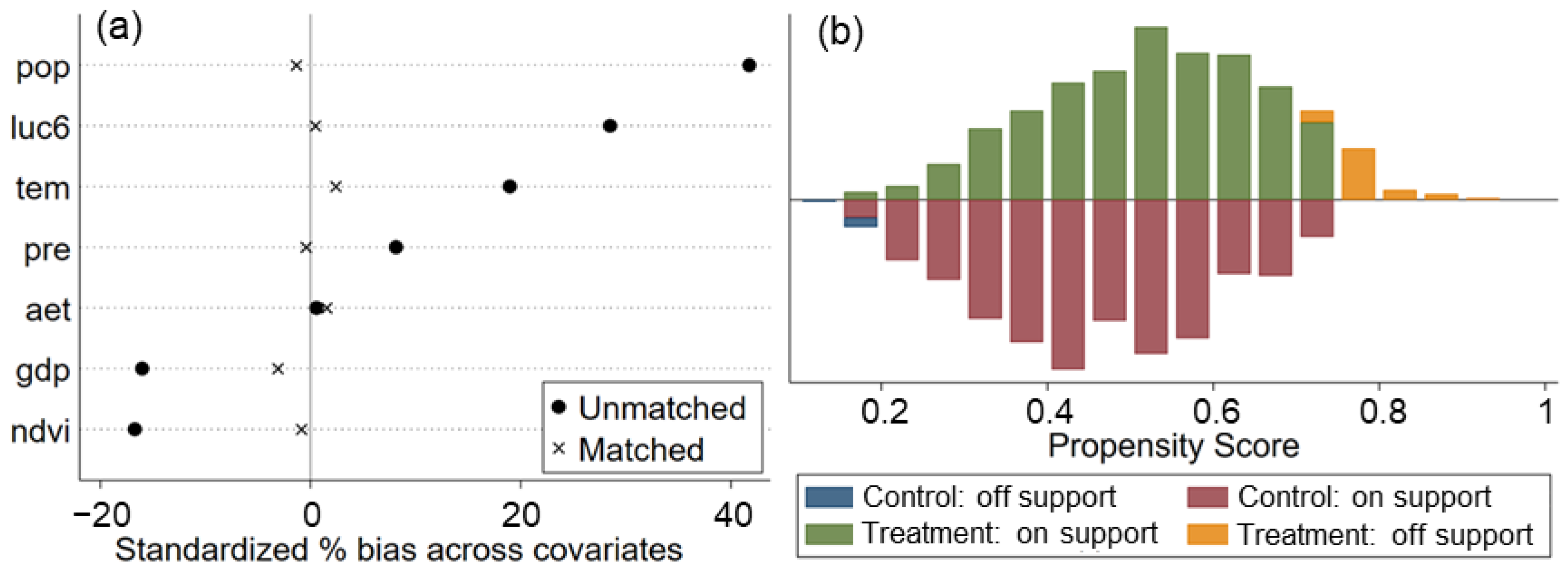
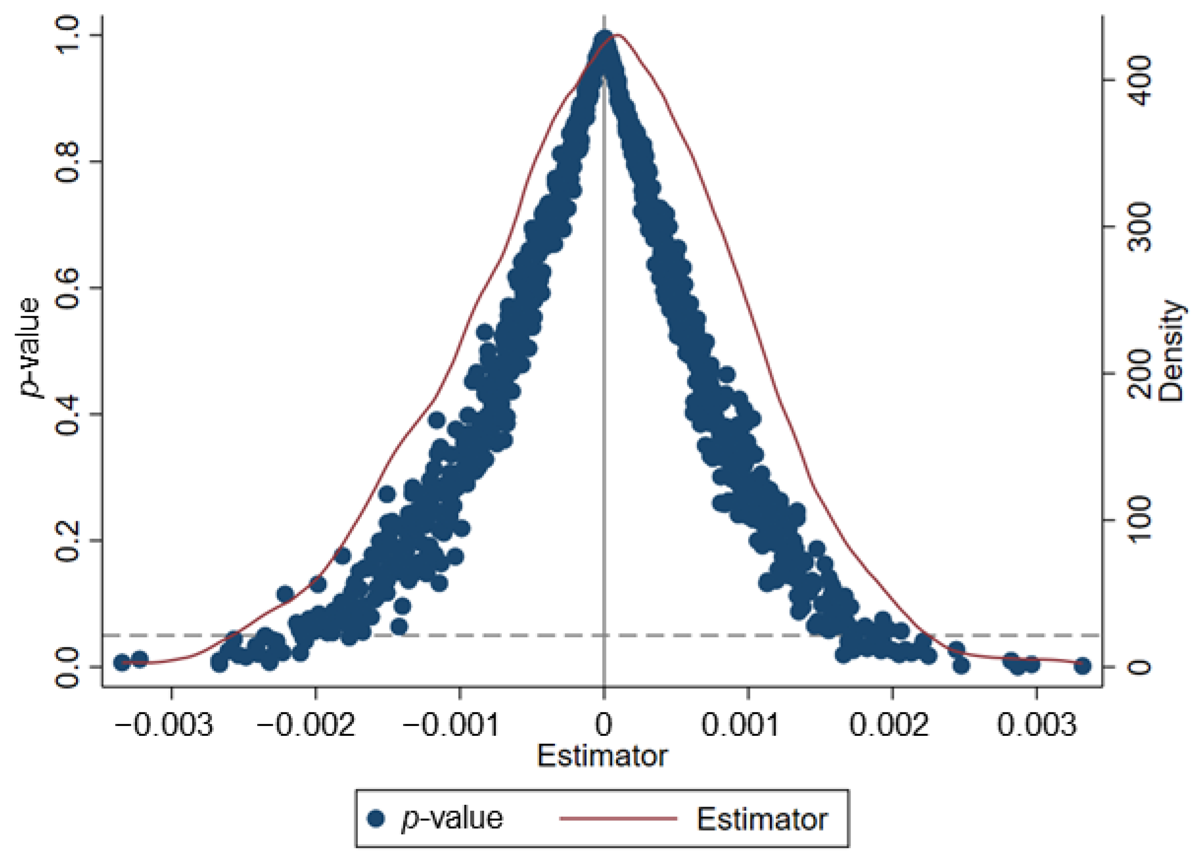
3.4. Identifying the Effect of Driving Factors via PSM-DID
4. Results
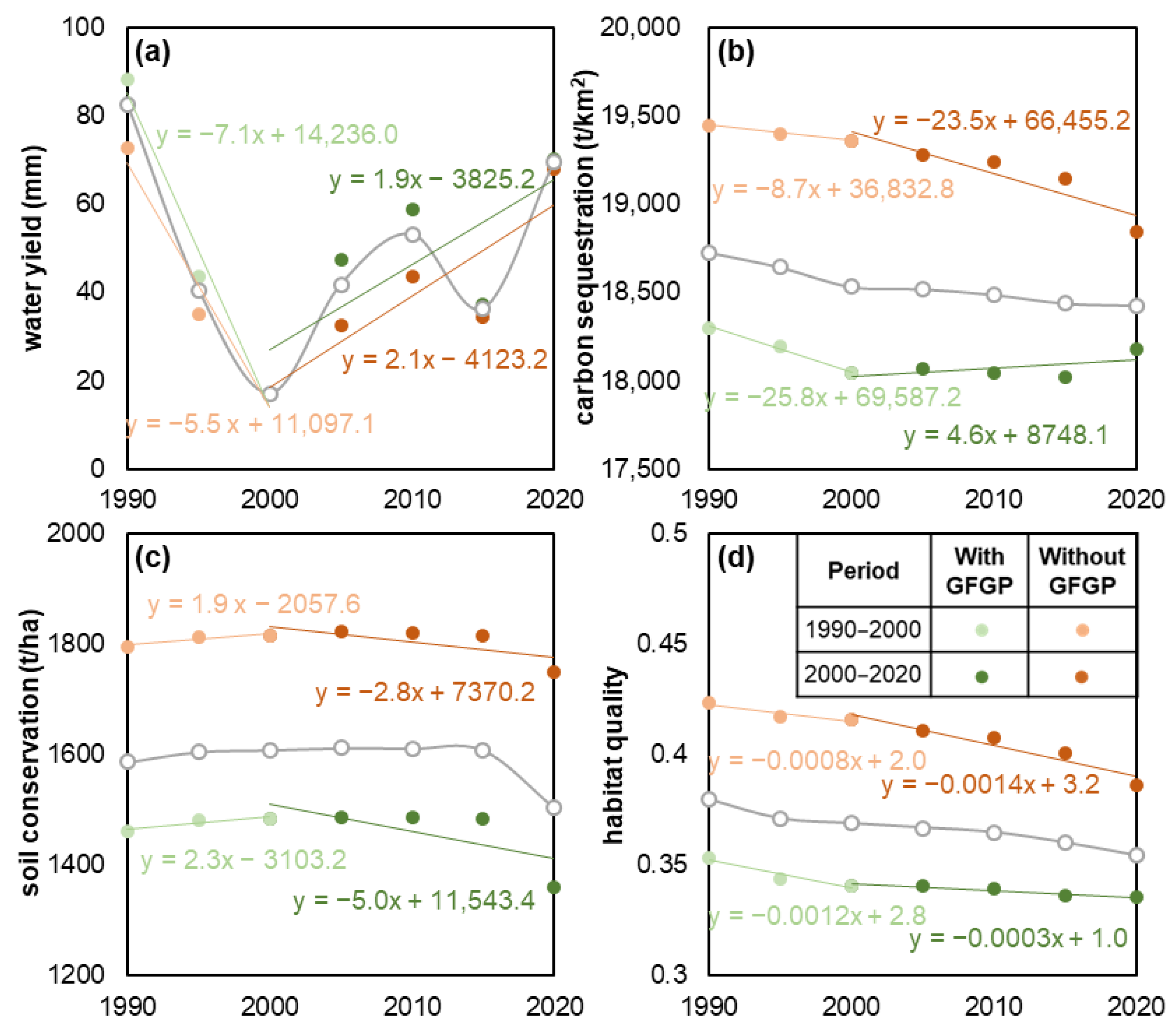
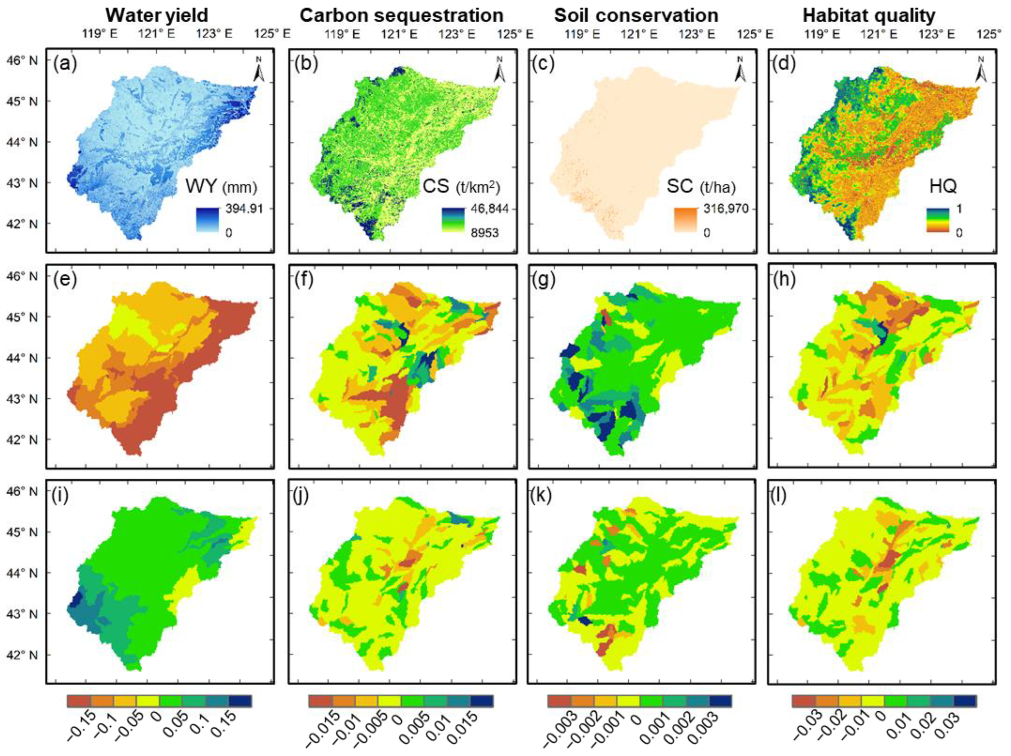
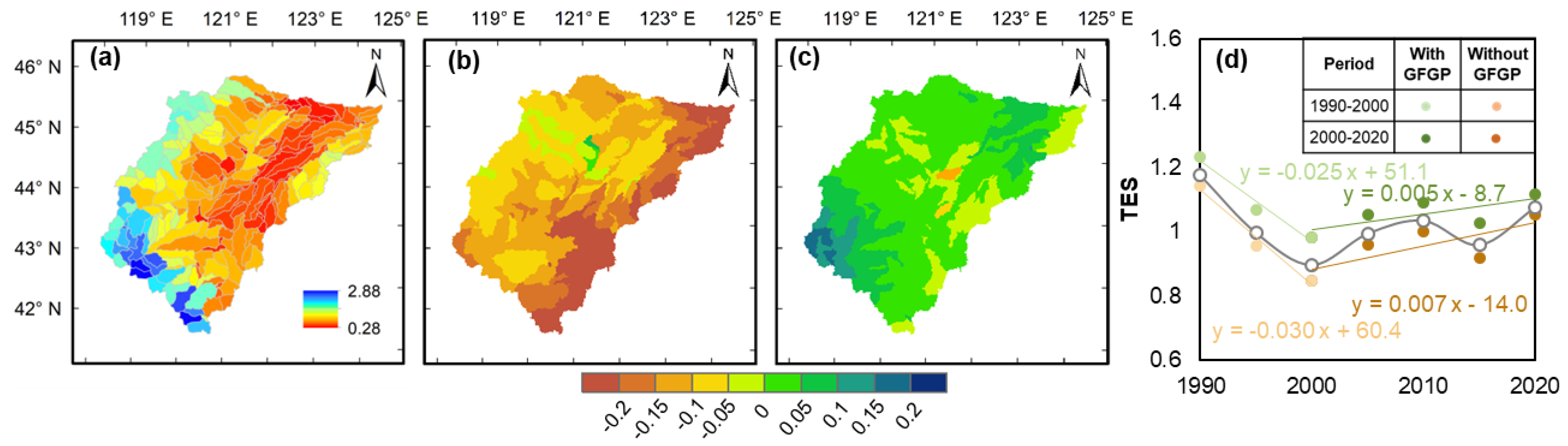
4.1. Temporal and Spatial Variation of Ecosystem Services
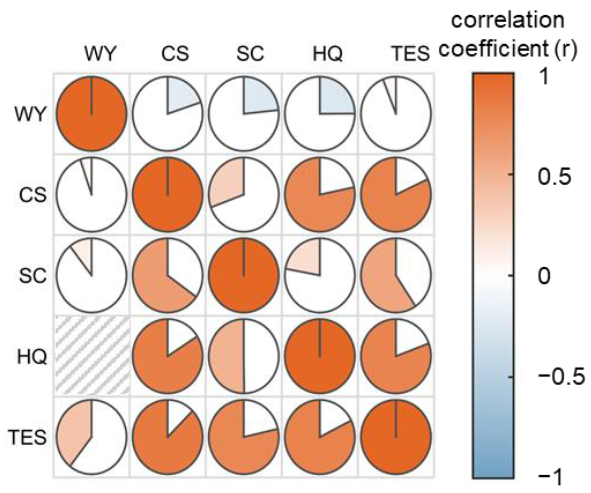
4.2. Tradeoff and Synergy among Ecosystem Services
4.3. Response of Ecosystem Services to Driving Factors
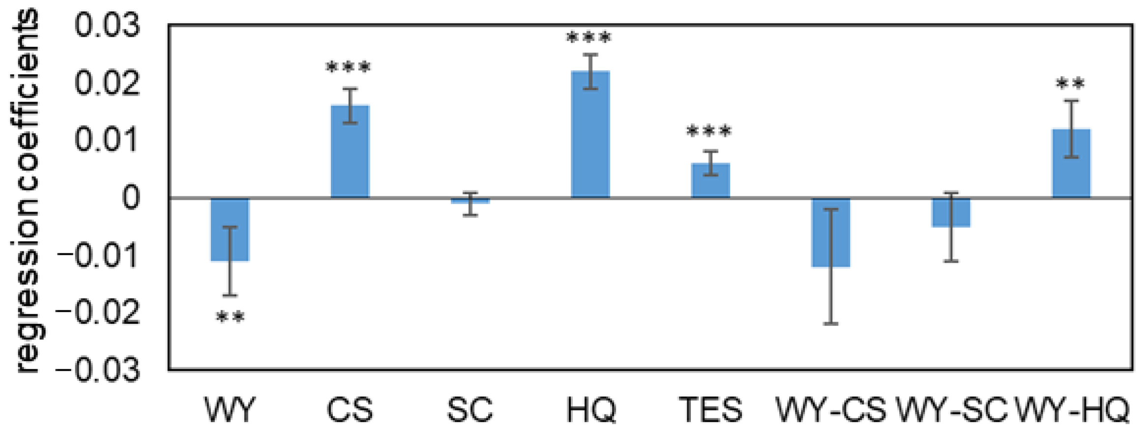
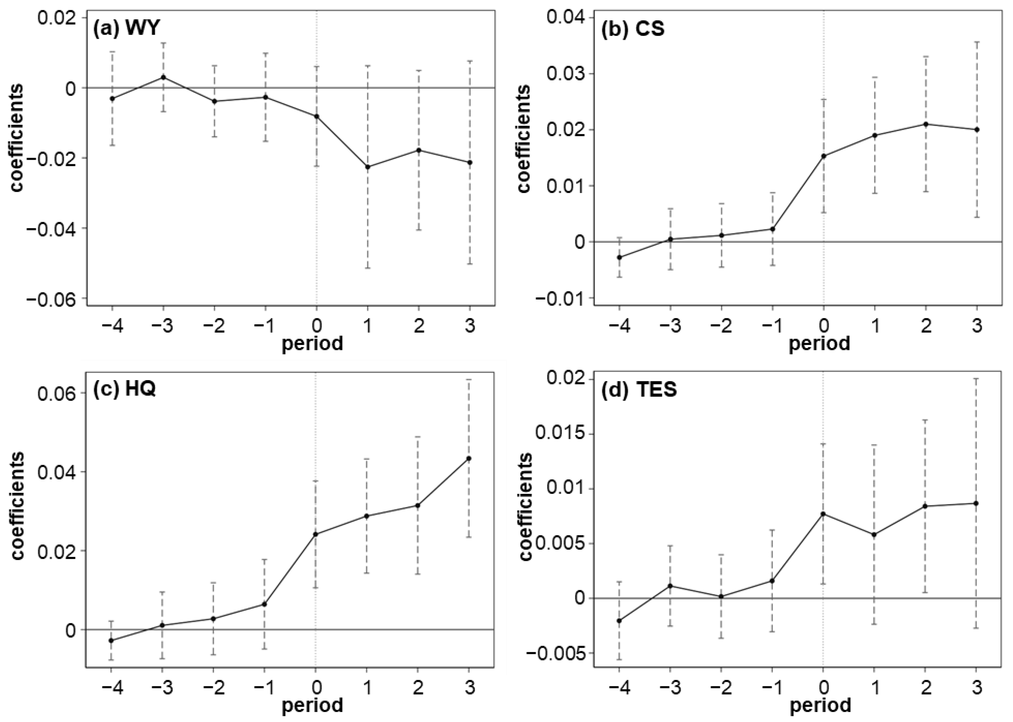
4.3.1. The Effect of the Grain-for-Green Program on Ecosystem Services
4.3.2. The Effect of the Control Variables on Ecosystem Services
5. Discussion
5.1. Contribution of Ecological Restoration to Ecosystem Services
5.2. Policy Implications
- (1)
- The negative effects of vegetation restoration policies on WY were nonnegligible, despite climatic factors increasing WY in the WLRB. The negative impacts of the revegetation policy were most focused on vegetation restoration, which would lead to soil water deficits for long-term vegetation growth [70]. Additionally, introduced plants would consume more soil water than native plants and affect the local water cycle [68,70]. Studies have confirmed that the runoff decline in the Loess Plateau region was associated with the GFGP by increasing net primary productivity and evapotranspiration [7,25,71]. The GFGP designer should consider the balance to guarantee food security and natural resources, maintain the function of water production in mountainous areas, and scientifically provide water resources for agriculture and cities in plain areas. Water resources in the plain area mainly maintain the balance of the ecological environment and grain supply.
- (2)
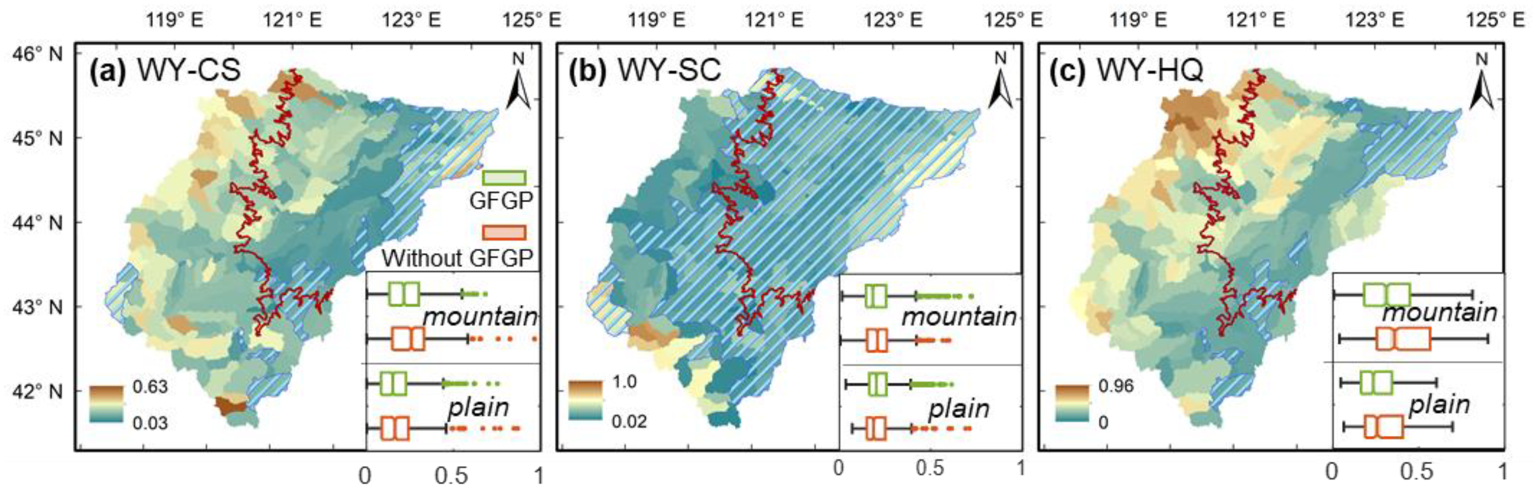
- To alleviate tradeoffs among WY and other ESs, the zonal management of GFGP should be paid more attention. Comprehensively understanding the synergistic or tradeoff relationships of ESs would help make decisions on managing land use and vegetation restoration [33,66]. The tradeoff between soil moisture and erosion control [72], water conservation, and biodiversity conservation [73], etc. have been widely discussed. Maximizing one ES may lead to a decrease in others, while exceeding the threshold may result in irreversible changes [3]. Significant tradeoff relationships among WY and other ESs were explored in our study. The mountain area was considered to be a hotspot of the tradeoff relationship, which was the major water supply and conservation area. In mountain areas, especially with strong tradeoff intensity, excessive forest restoration may exceed the water supply capacity and natural restoration. The Horqin sandy area of the WLRB, which has relatively sufficient water resources and is poor in CS and HQ, needs to improve the regional ESs by optimizing pasture management and planting local vegetation [74]. In the eastern plain of the WLRB, the water resource needs to be restored through water allocation and improving agricultural production capacity.
- (3)
- Future improvements of ESs required timely adjustments to policy implementation methodologies. Climate change is considered a major threat to ESs, while climate warming would aggravate the tradeoffs among ESs. Policymakers need to take this uncertainty and challenge into consideration. Moreover, in addition to environmental effects, the existing GFGP has economic effects, such as increasing farmers’ income and promoting nonagricultural employment [54,75]. The ecological damage caused by socioeconomic development can be reduced through industrial restructurings, such as developing tourism and planting economic forests.
5.3. Uncertainty and Limitations
6. Conclusions
- (1)
- During the pre-GFGP period (1990–2000), annual water yield decreased from 82.4 mm to 17.2 mm, and carbon sequestration and soil conservation were reduced in 70.8% and 79.7% of the subbasins. In the post-GFGP period (2000–2020), the WY started to recover, and the declining tendency of CS and HQ was halted in the group with GFGP. Spatially, the TES declined from south to north of the WLRB, peaking at 2.65 in the southwest corner of the basin and falling to its lowest value (nearly 0) in the central Horqin sandy area.
- (2)
- A synergistic relationship was shown among carbon sequestration, soil conservation, and habitat quality. The strongest correlation was found between carbon sequestration and habitat quality, with a partial correlation coefficient of 0.78. Water yield had a tradeoff relationship with other ESs, where were primarily present in the mountain area of the WLRB.
- (3)
- The GFGP was confirmed to have the greatest impact on enhancing habitat quality and carbon sequestration among the four ESs, while having an adverse impact on water yield and soil conservation. Air temperature and population density were major determinants for tradeoffs between water yield and other ESs. The methodology and implications provided in our study can provide guidance for regional ecological planning.
Author Contributions
Funding
Data Availability Statement
Acknowledgments
Conflicts of Interest
Appendix A

| Variable | Mean | Standard Deviation | Minimum | Median | Maximum |
|---|---|---|---|---|---|
| WY | 0.18 | 0.17 | 0 | 0.13 | 1 |
| CS | 0.3 | 0.13 | 0 | 0.29 | 1 |
| SC | 0.12 | 0.19 | 0 | 0.03 | 1 |
| HQ | 0.42 | 0.21 | 0 | 0.39 | 1 |
| TES | 0.26 | 0.13 | 0.05 | 0.23 | 0.78 |
| PRE | 0.4 | 0.18 | 0 | 0.39 | 1 |
| TEM | 0.7 | 0.21 | 0 | 0.77 | 1 |
| AET | 0.72 | 0.1 | 0 | 0.72 | 1 |
| NDVI | 0.39 | 0.13 | 0 | 0.38 | 1 |
| lnpop | 0.36 | 0.17 | 0 | 0.38 | 1 |
| lngdp | 0.26 | 0.13 | 0 | 0.25 | 1 |
| Urban land | 0.32 | 0.17 | 0 | 0.30 | 1 |

Appendix B

References
- Seppelt, R.; Dormann, C.F.; Eppink, F.V.; Lautenbach, S.; Schmidt, S. A quantitative review of ecosystem service studies: Approaches, shortcomings and the road ahead. J. Appl. Ecol. 2011, 48, 630–636. [Google Scholar] [CrossRef]
- Costanza, R.; d’Arge, R.; de Groot, R.; Farber, S.; Grasso, M.; Hannon, B.; Limburg, K.; Naeem, S.; O’Neill, R.V.; Paruelo, J.; et al. The value of the world’s ecosystem services and natural capital. Nature 1997, 387, 253–260. [Google Scholar] [CrossRef]
- Fu, B.; Zhang, L.; Xu, Z.; Zhao, Y.; Wei, Y.; Skinner, D. Ecosystem services in changing land use. J. Soils Sediments 2015, 15, 833–843. [Google Scholar] [CrossRef]
- Zheng, H.; Wang, L.; Peng, W.; Zhang, C.; Li, C.; Robinson, B.E.; Wu, X.; Kong, L.; Li, R.; Xiao, Y.; et al. Realizing the values of natural capital for inclusive, sustainable development: Informing China’s new ecological development strategy. Proc. Natl. Acad. Sci. USA 2019, 116, 8623–8628. [Google Scholar] [CrossRef]
- Yang, R.; Ren, F.; Xu, W.; Ma, X.; Zhang, H.; He, W. China’s ecosystem service value in 1992-2018: Pattern and anthropogenic driving factors detection using Bayesian spatiotemporal hierarchy model. J. Environ. Manag. 2022, 302, 114089. [Google Scholar] [CrossRef] [PubMed]
- UN Environment Programme. Available online: https://sdgs.un.org/un-system-sdg-implementation/united-nations-environment-programme-unep-49503 (accessed on 14 March 2023).
- Feng, X.; Fu, B.; Piao, S.; Wang, S.; Ciais, P.; Zeng, Z.; Lü, Y.; Zeng, Y.; Li, Y.; Jiang, X.; et al. Revegetation in China’s Loess Plateau is approaching sustainable water resource limits. Nat. Clim. Chang. 2016, 6, 1019–1022. [Google Scholar] [CrossRef]
- Wang, Y.; Zhao, J.; Fu, J.; Wei, W. Effects of the Grain for Green Program on the water ecosystem services in an arid area of China—Using the Shiyang River Basin as an example. Ecol. Indic. 2019, 104, 659–668. [Google Scholar] [CrossRef]
- Ma, S.; Qiao, Y.-P.; Jiang, J.; Wang, L.-J.; Zhang, J.-C. Incorporating the implementation intensity of returning farmland to lakes into policymaking and ecosystem management: A case study of the Jianghuai Ecological Economic Zone, China. J. Clean. Prod. 2021, 306, 127284. [Google Scholar] [CrossRef]
- Zhu, W.; Gao, Y.; Zhang, H.; Liu, L. Optimization of the land use pattern in Horqin Sandy Land by using the CLUMondo model and Bayesian belief network. Sci. Total Environ. 2020, 739, 139929. [Google Scholar] [CrossRef]
- Bai, M.; Mo, X.; Mo, S.; Feng, J. Separating climate change and vegetation dynamics contributions to soil drying over drylands of China: A case study in the West Liao River Basin. Ecohydrology 2022, 15. [Google Scholar] [CrossRef]
- Smith, P.; Ashmore, M.R.; Black, H.I.J.; Burgess, P.J.; Evans, C.D.; Quine, T.A.; Thomson, A.M.; Hicks, K.; Orr, H.G.; Angeler, D. REVIEW: The role of ecosystems and their management in regulating climate, and soil, water and air quality. J. Appl. Ecol. 2013, 50, 812–829. [Google Scholar] [CrossRef]
- Dou, H.; Li, X.; Gong, J.; Wang, H.; Tian, Y.; Xuan, X.; Wang, K. Enhanced ecosystem services in China’s Xilingol steppe during 2000–2015: Towards sustainable agropastoralism management. Remote Sens. 2022, 14, 738. [Google Scholar] [CrossRef]
- Yang, D.; Liu, W.; Tang, L.; Chen, L.; Li, X.; Xu, X. Estimation of water provision service for monsoon catchments of South China: Applicability of the InVEST model. Landsc. Urban Plan 2019, 182, 133–143. [Google Scholar] [CrossRef]
- Tian, Y.; Wang, S.; Bai, X.; Luo, G.; Xu, Y. Trade-offs among ecosystem services in a typical Karst watershed, SW China. Sci. Total Environ. 2016, 566, 1297–1308. [Google Scholar] [CrossRef]
- Benra, F.; De Frutos, A.; Gaglio, M.; Álvarez-Garretón, C.; Felipe-Lucia, M.; Bonn, A. Mapping water ecosystem services: Evaluating InVEST model predictions in data scarce regions. Environ. Model. Softw. 2021, 138, 104982. [Google Scholar] [CrossRef]
- Vigerstol, K.L.; Aukema, J.E. A comparison of tools for modeling freshwater ecosystem services. J. Environ. Manag. 2011, 92, 2403–2409. [Google Scholar] [CrossRef]
- Radoglou Grammatikis, P.; Sarigiannidis, P.; Efstathopoulos, G.; Panaousis, E. ARIES: A Novel Multivariate Intrusion Detection System for Smart Grid. Sensors 2020, 20, 5305. [Google Scholar] [CrossRef]
- Caro, C.; Marques, J.C.; Cunha, P.P.; Teixeira, Z. Ecosystem services as a resilience descriptor in habitat risk assessment using the InVEST model. Ecol. Indic. 2020, 115, 106426. [Google Scholar] [CrossRef]
- Daily, G.C.; Matson, P.A. Ecosystem services: From theory to implementation. Proc. Natl. Acad. Sci. USA 2008, 105, 9455–9456. [Google Scholar] [CrossRef]
- Martínez-Harms, M.J.; Balvanera, P. Methods for mapping ecosystem service supply: A review. Int. J. Biodivers. Sci. Ecosyst. Serv. Manag. 2012, 8, 17–25. [Google Scholar] [CrossRef]
- Hu, Y.; Peng, J.; Liu, Y.; Tian, L. Integrating ecosystem services trade-offs with paddy land-to-dry land decisions: A scenario approach in Erhai Lake Basin, southwest China. Sci. Total Environ. 2018, 625, 849–860. [Google Scholar] [CrossRef] [PubMed]
- Xi, Y.; Peng, S.; Liu, G.; Ducharne, A.; Ciais, P.; Prigent, C.; Li, X.; Tang, X. Trade-off between tree planting and wetland conservation in China. Nat. Commun. 2022, 13, 1967. [Google Scholar] [CrossRef] [PubMed]
- Jia, X.; Fu, B.; Feng, X.; Hou, G.; Liu, Y.; Wang, X. The tradeoff and synergy between ecosystem services in the Grain-for-Green areas in Northern Shaanxi, China. Ecol. Indic. 2014, 43, 103–113. [Google Scholar] [CrossRef]
- Feng, Q.; Zhao, W.; Hu, X.; Liu, Y.; Daryanto, S.; Cherubini, F. Trading-off ecosystem services for better ecological restoration: A case study in the Loess Plateau of China. J. Clean. Prod. 2020, 257, 120469. [Google Scholar] [CrossRef]
- Peng, J.; Hu, X.; Wang, X.; Meersmans, J.; Liu, Y.; Qiu, S. Simulating the impact of Grain-for-Green Programme on ecosystem services trade-offs in Northwestern Yunnan, China. Ecosyst. Serv. 2019, 39, 100998. [Google Scholar] [CrossRef]
- Bradford, J.B.; D’Amato, A.W. Recognizing trade-offs in multi-objective land management. Front. Ecol. Environ. 2012, 10, 210–216. [Google Scholar] [CrossRef]
- Fan, Y.; Gan, L.; Hong, C.; Jessup, L.H.; Jin, X.; Pijanowski, B.C.; Sun, Y.; Lv, L. Spatial identification and determinants of trade-offs among multiple land use functions in Jiangsu Province, China. Sci. Total Environ. 2021, 772, 145022. [Google Scholar] [CrossRef]
- Liu, Z.; Wu, R.; Chen, Y.; Fang, C.; Wang, S. Factors of ecosystem service values in a fast-developing region in China: Insights from the joint impacts of human activities and natural conditions. J. Clean. Prod. 2021, 297. [Google Scholar] [CrossRef]
- Yang, S.; Zhao, W.; Liu, Y.; Wang, S.; Wang, J.; Zhai, R. Influence of land use change on the ecosystem service trade-offs in the ecological restoration area: Dynamics and scenarios in the Yanhe watershed, China. Sci. Total Environ. 2018, 644, 556–566. [Google Scholar] [CrossRef]
- Li, P.; Sheng, M.; Yang, D.; Tang, L. Evaluating flood regulation ecosystem services under climate, vegetation and reservoir influences. Ecol. Indic. 2019, 107. [Google Scholar] [CrossRef]
- Pham, H.V.; Sperotto, A.; Torresan, S.; Acuña, V.; Jorda-Capdevila, D.; Rianna, G.; Marcomini, A.; Critto, A. Coupling scenarios of climate and land-use change with assessments of potential ecosystem services at the river basin scale. Ecosyst. Serv. 2019, 40, 101045. [Google Scholar] [CrossRef]
- Wang, Y.; Dai, E. Spatial-temporal changes in ecosystem services and the trade-off relationship in mountain regions: A case study of Hengduan Mountain region in Southwest China. J. Clean. Prod. 2020, 264, 121573. [Google Scholar] [CrossRef]
- Sun, X.; Zhu, B.; Zhang, S.; Zeng, H.; Li, K.; Wang, B.; Dong, Z.; Zhou, C. New indices system for quantifying the nexus between economic-social development, natural resources consumption, and environmental pollution in China during 1978–2018. Sci. Total Environ. 2022, 804, 150180. [Google Scholar] [CrossRef]
- Fang, Z.; Bai, Y.; Jiang, B.; Alatalo, J.M.; Liu, G.; Wang, H. Quantifying variations in ecosystem services in altitude-associated vegetation types in a tropical region of China. Sci. Total Environ. 2020, 726, 138565. [Google Scholar] [CrossRef]
- Houghton, R.A.; House, J.I.; Pongratz, J.; van der Werf, G.R.; DeFries, R.S.; Hansen, M.C.; Le Quere, C.; Ramankutty, N. Carbon emissions from land use and land-cover change. Biogeosciences 2012, 9, 5125–5142. [Google Scholar] [CrossRef]
- Foley, J.A.; Defries, R.; Asner, G.P.; Barford, C.; Bonan, G.; Carpenter, S.R.; Chapin, F.S.; Coe, M.T.; Daily, G.C.; Gibbs, H.K.; et al. Global consequences of land use. Science 2005, 309, 570–574. [Google Scholar] [CrossRef]
- Huang, Y.; Matsumoto, K.I. Drivers of the change in carbon dioxide emissions under the progress of urbanization in 30 provinces in China: A decomposition analysis. J. Clean. Prod. 2021, 322, 129000. [Google Scholar] [CrossRef]
- Liang, S.; Li, Y.; Zhang, X.; Sun, Z.; Sun, N.; Duan, Y.; Xu, M.; Wu, L. Response of crop yield and nitrogen use efficiency for wheat-maize cropping system to future climate change in northern China. Agric. For. Meteorol. 2018, 262, 310–321. [Google Scholar] [CrossRef]
- Liu, J.; Li, S.; Ouyang, Z.; Tam, C.; Chen, X. Ecological and socioeconomic effects of China’s policies for ecosystem services. Proc. Natl. Acad. Sci. USA 2008, 105, 9477–9482. [Google Scholar] [CrossRef]
- Yuan, J.; Ouyang, Z.; Zheng, H.; Xu, W. Effects of different grassland restoration approaches on soil properties in the southeastern Horqin sandy land, northern China. Appl. Soil Ecol. 2012, 61, 34–39. [Google Scholar] [CrossRef]
- Wang, L.-J.; Ma, S.; Jiang, J.; Zhao, Y.-G.; Zhang, J.-C. Spatiotemporal Variation in Ecosystem Services and Their Drivers among Different Landscape Heterogeneity Units and Terrain Gradients in the Southern Hill and Mountain Belt, China. Remote Sens. 2021, 13, 1375. [Google Scholar] [CrossRef]
- Hu, B.; Zhang, Z.; Han, H.; Li, Z.; Cheng, X.; Kang, F.; Wu, H. The Grain for Green Program intensifies trade-offs between ecosystem services in midwestern Shanxi, China. Remote Sens. 2021, 13, 3966. [Google Scholar] [CrossRef]
- Liu, Y.; Lu, Y.; Fu, B.; Harris, P.; Wu, L. Quantifying the spatio-temporal drivers of planned vegetation restoration on ecosystem services at a regional scale. Sci. Total Environ. 2019, 650, 1029–1040. [Google Scholar] [CrossRef] [PubMed]
- Wang, J.; Peng, J.; Zhao, M.; Liu, Y.; Chen, Y. Significant trade-off for the impact of Grain-for-Green Programme on ecosystem services in North-western Yunnan, China. Sci. Total Environ. 2017, 574, 57–64. [Google Scholar] [CrossRef]
- Wang, X.; Zhang, X.; Feng, X.; Liu, S.; Yin, L.; Chen, Y. Trade-offs and Synergies of Ecosystem Services in Karst Area of China Driven by Grain-for-Green Program. Chin. Geogr. Sci. 2020, 30, 101–114. [Google Scholar] [CrossRef]
- Liu, M.; Jia, Y.; Zhao, J.; Shen, Y.; Pei, H.; Zhang, H.; Li, Y. Revegetation projects significantly improved ecosystem service values in the agro-pastoral ecotone of northern China in recent 20 years. Sci. Total Environ. 2021, 788, 147756. [Google Scholar] [CrossRef] [PubMed]
- Qian, D.; Du, Y.; Li, Q.; Guo, X.; Cao, G. Alpine grassland management based on ecosystem service relationships on the southern slopes of the Qilian Mountains, China. J. Environ. Manag. 2021, 288, 112447. [Google Scholar] [CrossRef]
- Li, Y.; Piao, S.; Li, L.Z.X.; Chen, A.; Wang, X.; Ciais, P.; Huang, L.; Lian, X.; Peng, S.; Zeng, Z.; et al. Divergent hydrological response to large-scale afforestation and vegetation greening in China. Scince Adv. 2018, 4, eaar4182. [Google Scholar] [CrossRef]
- Wu, X.; Wang, S.; Fu, B.; Liu, Y.; Zhu, Y. Land use optimization based on ecosystem service assessment: A case study in the Yanhe watershed. Land Use Policy 2018, 72, 303–312. [Google Scholar] [CrossRef]
- Wang, X.; Wu, J.; Liu, Y.; Hai, X.; Shanguan, Z.; Deng, L. Driving factors of ecosystem services and their spatiotemporal change assessment based on land use types in the Loess Plateau. J. Environ. Manag. 2022, 311, 114835. [Google Scholar] [CrossRef]
- Wang, Y.; Wang, H.; Zhang, J.; Liu, G.; Fang, Z.; Wang, D. Exploring interactions in water-related ecosystem services nexus in Loess Plateau. J. Environ. Manag. 2023, 336, 117550. [Google Scholar] [CrossRef]
- Wang, K.-L.; Pang, S.-Q.; Zhang, F.-Q.; Miao, Z. Does high-speed rail improve China’s urban environmental efficiency? Empirical evidence from a quasi-natural experiment. Environ. Sci. Pollut. Res. 2022, 29, 31901–31922. [Google Scholar] [CrossRef] [PubMed]
- Hayes, T.; Murtinho, F.; Wolff, H.; Lopez-Sandoval, M.F.; Salazar, J. Effectiveness of payment for ecosystem services after loss and uncertainty of compensation. Nat. Sustain. 2022, 5, 81–88. [Google Scholar] [CrossRef]
- Xu, Z.; Dai, Y.; Liu, W. Does environmental audit help to improve water quality? Evidence from the China National Environmental Monitoring Centre. Sci. Total Environ. 2022, 823, 153485. [Google Scholar] [CrossRef]
- Peng, S. 1-km Monthly Precipitation Dataset for China (1901–2020); National Tibetan Plateau Data Center: Beijing, China, 2020. [Google Scholar] [CrossRef]
- Meng, X.; Wang, H. Siol Map Based Harmonized World Soil Database (v1.2); National Tibetan Plateau Data Center: Beijing, China, 2018. [Google Scholar]
- Sharp, R.; Tallis, H.T.; Ricketts, T.; Guerry, A.D.; Wood, S.A.; Chaplin-Kramer, R.; Foster, J.; Arkema, K.; Toft, J.; Rogers, L.; et al. VEST + VERSION + User’s Guide; The Natural Capital Project; Stanford University: Stanford, CA, USA; University of Minnesota: Minneapolis, MN, USA; The Nature Conservancy: Arlington County, VA, USA; World Wildlife Fund: Gland, Switzerland, 2018. [Google Scholar]
- Wu, Y.F.; Zhang, X.; Li, C.; Xu, Y.; Hao, F.H.; Yin, G.D. Ecosystem service trade-offs and synergies under influence of climate and land cover change in an afforested semiarid basin, China. Ecol. Eng. 2021, 159, 125838. [Google Scholar] [CrossRef]
- Zhang, Y.; Liu, Y.; Zhang, Y.; Liu, Y.; Zhang, G.; Chen, Y. On the spatial relationship between ecosystem services and urbanization: A case study in Wuhan, China. Sci. Total Env. 2018, 637, 780–790. [Google Scholar] [CrossRef]
- Qing, L.; Yong, Z.; Cunningham, M.A.; Tao, X. Spatio-Temporal Changes in Wildlife Habitat Quality in the Middle and Lower Reaches of the Yangtze River from 1980 to 2100 Based on the InVEST Model. J. Resour. Ecol. 2021, 12. [Google Scholar] [CrossRef]
- Baba, K.; Shibata, R.; Sibuya, M. Partial Correlation and Conditional Correlation as Measures of Conditional Independence. Aust. N. Z. J. Stat. 2004, 46, 657–664. [Google Scholar] [CrossRef]
- Piao, S.; Wang, X.; Park, T.; Chen, C.; Lian, X.; He, Y.; Bjerke, J.W.; Chen, A.; Ciais, P.; Tømmervik, H.; et al. Characteristics, drivers and feedbacks of global greening. Nat. Rev. Earth Environ. 2019, 1, 14–27. [Google Scholar] [CrossRef]
- Yang, D.; Yang, Y.; Xia, J. Hydrological cycle and water resources in a changing world: A review. Geogr. Sustain. 2021, 2, 115–122. [Google Scholar] [CrossRef]
- Cumming, G.S.; Buerkert, A.; Hoffmann, E.M.; Schlecht, E.; von Cramon-Taubadel, S.; Tscharntke, T. Implications of agricultural transitions and urbanization for ecosystem services. Nature 2014, 515, 50–57. [Google Scholar] [CrossRef] [PubMed]
- Luo, Y.; Lu, Y.; Fu, B.; Zhang, Q.; Li, T.; Hu, W.; Comber, A. Half century change of interactions among ecosystem services driven by ecological restoration: Quantification and policy implications at a watershed scale in the Chinese Loess Plateau. Sci. Total Environ. 2019, 651, 2546–2557. [Google Scholar] [CrossRef] [PubMed]
- Yan, K.; Wang, W.; Li, Y.; Wang, X.; Jin, J.; Jiang, J.; Yang, H.; Wang, L. Identifying priority conservation areas based on ecosystem services change driven by Natural Forest Protection Project in Qinghai province, China. J. Clean. Prod. 2022, 362, 132453. [Google Scholar] [CrossRef]
- Cao, S.; Chen, L.; Shankman, D.; Wang, C.; Wang, X.; Zhang, H. Excessive reliance on afforestation in China’s arid and semi-arid regions: Lessons in ecological restoration. Earth-Sci. Rev. 2011, 104, 240–245. [Google Scholar] [CrossRef]
- Yang, L.; Li, X.; Li, X.; Su, Z.; Zhang, C.; Zhang, H. Bioremediation of chlorimuron-ethyl-contaminated soil by Hansschlegelia sp. strain CHL1 and the changes of indigenous microbial population and N-cycling function genes during the bioremediation process. J. Hazard. Mater. 2014, 274, 314–321. [Google Scholar] [CrossRef] [PubMed]
- Yang, L.; Wei, W.; Chen, L.; Chen, W.; Wang, J. Response of temporal variation of soil moisture to vegetation restoration in semi-arid Loess Plateau, China. Catena 2014, 115, 123–133. [Google Scholar] [CrossRef]
- Sun, W.; Song, X.; Mu, X.; Gao, P.; Wang, F.; Zhao, G. Spatiotemporal vegetation cover variations associated with climate change and ecological restoration in the Loess Plateau. Agric. For. Meteorol. 2015, 209, 87–99. [Google Scholar] [CrossRef]
- Feng, Q.; Zhao, W.; Fu, B.; Ding, J.; Wang, S. Ecosystem service trade-offs and their influencing factors: A case study in the Loess Plateau of China. Sci. Total Environ. 2017, 607, 1250–1263. [Google Scholar] [CrossRef]
- Xu, X.; Yang, G.; Tan, Y.; Liu, J.; Hu, H. Ecosystem services trade-offs and determinants in China’s Yangtze River Economic Belt from 2000 to 2015. Sci. Total Environ. 2018, 634, 1601–1614. [Google Scholar] [CrossRef]
- Li, Y.; Cao, Z.; Long, H.; Liu, Y.; Li, W. Dynamic analysis of ecological environment combined with land cover and NDVI changes and implications for sustainable urban–rural development: The case of Mu Us Sandy Land, China. J. Clean. Prod. 2017, 142, 697–715. [Google Scholar] [CrossRef]
- Gao, J.; Li, F.; Gao, H.; Zhou, C.; Zhang, X. The impact of land-use change on water-related ecosystem services: A study of the Guishui River Basin, Beijing, China. J. Clean. Prod. 2017, 163, S148–S155. [Google Scholar] [CrossRef]
- Venkatesh, K.; John, R.; Chen, J.; Jarchow, M.; Amirkhiz, R.G.; Giannico, V.; Saraf, S.; Jain, K.; Kussainova, M.; Yuan, J. Untangling the impacts of socioeconomic and climatic changes on vegetation greenness and productivity in Kazakhstan. Environ. Res. Lett. 2022, 17. [Google Scholar] [CrossRef]
- Chetty, R.; Looney, A.; Kroft, K. Salience and Taxation: Theory and Evidence. Am. Econ. Rev. 2009, 99, 1145–1177. [Google Scholar] [CrossRef]


| ESs | Description | Mathematical Expression |
|---|---|---|
| Water yield (WY) | Water produced by a watershed and arriving in streams | where , , and is the annual water yield, actual evapotranspiration, and precipitation of pixel |
| Carbon sequestration (CS) | The amount of carbon currently stored in a landscape or the amount of carbon sequestered over time | where , , , and are the carbon pools of above-ground biomass, below-ground biomass, soil organic matter, and dead organic matter |
| Soil conservation (SC) | Erosion control ability of the ecosystem to prevent soil loss and the ability to store and maintain sediment | where is the soil conservation capacity, is is the rainfall erosivity (MJ mm(ha·h·yr)−1), is the soil erodibility (ton·ha·h(MJ·ha·mm)−1), is a slope length gradient factor (unitless), is a cover-management factor (unitless), and is a support practice factor (unitless) in pixel i [58] |
| Habitat quality (HQ) | Ability to provide resources and environmental conditions for the survival and development of species or populations | where is the habitat quality in pixel i, H is the habitat suitability of different types of LUCC, and are the level of threat and half-saturation constant, and Z is the implicit parameter of the model [60,61] |
| Model | (1) | (2) | (3) | (4) | (5) | (6) | (7) | (8) |
|---|---|---|---|---|---|---|---|---|
| WY | CS | SC | HQ | TES | WY-CS | WY-SC | WY-HQ | |
| GFGP | −0.011 ** | 0.016 *** | −0.001 | 0.022 *** | 0.006 *** | −0.012 | −0.005 | 0.012 ** |
| (0.006) | (0.003) | (0.002) | (0.003) | (0.002) | (0.010) | (0.006) | (0.005) | |
| PRE | 1.281 *** | 0.060 ** | −0.009 | −0.001 | 0.333 *** | 0.312 * | 0.455 *** | 0.002 |
| (0.180) | (0.030) | (0.011) | (0.013) | (0.039) | (0.162) | (0.097) | (0.074) | |
| TEM | 0.072 | 0.119 *** | 0.120 *** | 0.029 | 0.085 *** | 1.052 *** | 0.671 *** | 0.641 *** |
| (0.083) | (0.039) | (0.024) | (0.035) | (0.027) | (0.177) | (0.099) | (0.081) | |
| AET | −0.982 *** | −0.098 * | 0.014 | 0.034 | −0.258 *** | −0.779 *** | −0.489 *** | −0.164 |
| (0.350) | (0.057) | (0.017) | (0.022) | (0.077) | (0.280) | (0.163) | (0.107) | |
| NDVI | −0.095 ** | −0.020 | 0.031 *** | −0.044 | −0.032 ** | −0.020 | 0.019 | −0.021 |
| (0.039) | (0.016) | (0.011) | (0.027) | (0.013) | (0.053) | (0.037) | (0.034) | |
| lnpop | −0.080 * | 0.020 | 0.040 ** | −0.032 | −0.013 | 0.349 *** | 0.253 *** | 0.256 *** |
| (0.047) | (0.021) | (0.016) | (0.023) | (0.015) | (0.096) | (0.058) | (0.051) | |
| lngdp | 0.140 | −0.042 | 0.017 | −0.097 *** | 0.004 | 0.014 | −0.122 | −0.170 ** |
| (0.119) | (0.034) | (0.014) | (0.035) | (0.033) | (0.171) | (0.109) | (0.077) | |
| Urban land | 0.076 | −0.052 | −0.102 ** | −0.146 *** | −0.056 ** | −0.107 | −0.093 | −0.112 ** |
| (0.084) | (0.034) | (0.042) | (0.039) | (0.027) | (0.097) | (0.071) | (0.049) | |
| Constant | 0.297 | 0.306 *** | 0.042 | 0.498 *** | 0.286 *** | −0.151 | −0.082 | 0.029 |
| (0.197) | (0.038) | (0.026) | (0.034) | (0.046) | (0.208) | (0.124) | (0.078) | |
| Observations | 1465 | 1465 | 1465 | 1465 | 1465 | 1465 | 1465 | 1465 |
| Adjusted R2 | 0.940 | 0.980 | 0.996 | 0.989 | 0.988 | 0.579 | 0.729 | 0.928 |
Disclaimer/Publisher’s Note: The statements, opinions and data contained in all publications are solely those of the individual author(s) and contributor(s) and not of MDPI and/or the editor(s). MDPI and/or the editor(s) disclaim responsibility for any injury to people or property resulting from any ideas, methods, instructions or products referred to in the content. |
© 2023 by the authors. Licensee MDPI, Basel, Switzerland. This article is an open access article distributed under the terms and conditions of the Creative Commons Attribution (CC BY) license (https://creativecommons.org/licenses/by/4.0/).
Share and Cite
Xu, Y.; Yang, D.; Tang, L.; Qiao, Z.; Ma, L.; Chen, M. Exploring the Impact of Grain-for-Green Program on Trade-Offs and Synergies among Ecosystem Services in West Liao River Basin, China. Remote Sens. 2023, 15, 2490. https://doi.org/10.3390/rs15102490
Xu Y, Yang D, Tang L, Qiao Z, Ma L, Chen M. Exploring the Impact of Grain-for-Green Program on Trade-Offs and Synergies among Ecosystem Services in West Liao River Basin, China. Remote Sensing. 2023; 15(10):2490. https://doi.org/10.3390/rs15102490
Chicago/Turabian StyleXu, Yang, Dawen Yang, Lihua Tang, Zixu Qiao, Long Ma, and Min Chen. 2023. "Exploring the Impact of Grain-for-Green Program on Trade-Offs and Synergies among Ecosystem Services in West Liao River Basin, China" Remote Sensing 15, no. 10: 2490. https://doi.org/10.3390/rs15102490
APA StyleXu, Y., Yang, D., Tang, L., Qiao, Z., Ma, L., & Chen, M. (2023). Exploring the Impact of Grain-for-Green Program on Trade-Offs and Synergies among Ecosystem Services in West Liao River Basin, China. Remote Sensing, 15(10), 2490. https://doi.org/10.3390/rs15102490